Quantum Bose and Fermi gases with large negative scattering length in the 2-body S-matrix approximation

Abstract

We study both Bose and Fermi gases at finite temperature and density in an approximation that sums an infinite number of many body processes that are reducible to 2-body scatterings. This is done for arbitrary negative scattering length, which interpolates between the ideal and unitary gas limits. In the unitary limit, we compute the first four virial coefficients within our approximation. The second virial coefficient is exact, and we extend the previously known result for fermions to bosons, and also for both bosons and fermions for the upper branch on the other side of unitarity (infinitely large positive scattering length). Assuming bosons can exist in a meta-stable state before undergoing mechanical collapse, we map out the critical temperatures for strongly coupled Bose-Einstein condensation as a function of scattering length.

I Introduction

The growing amount of increasingly accurate data from experiments on cold atoms kett1 ; bloch1 ; chin1 ; nascimb1 ; Werner ; hori1 poses particularly interesting challenges for theorists to develop new methods. This is especially true for experiments where the scattering length can be tuned to vary anywhere between $\pm\infty$ using Feshbach resonances. Monte-Carlo methods have been developed sufficiently that excellent agreement with experiments has now been achieved ming1 ; Proko ; bulga1 ; bulga2 . Recent reviews are Castin ; DrumRev . Nevertheless, the development of new analytical methods, though approximate, continues to be a worthwhile pursuit because they can afford new insights into the underlying many-body physics.

One such method has been developed by one of us, and is based entirely on the zero temperature S-matrix PyeTon . It is reminiscent, in fact was modeled after, the thermodynamical Bethe ansatz equations of Yang and Yang YangYang . The ingredients are the same: the occupation numbers are parametrized in an ideal gas form, but with the one-particle energy replaced by a pseudo-energy $\varepsilon({\bf k})$. The latter satisfies an integral equation with a kernel based on the logarithm of the 2-body S-matrix at zero temperature, and there is a simple expression for the free energy at finite temperature and density. Whereas for integrable theories in 1 spatial dimension the thermodynamic Bethe ansatz is exact because of the factorizability of the many-body S-matrix, the formalism in PyeTon is certainly an approximation. Nevertheless it has certain desirable features, such as the fact that the 2-body S-matrix can be calculated exactly in non-relativistic theories, and has been demonstrated to give reasonably good results in some regimes. For instance, it was applied to the so-called unitary limit in 3 dimensions where the scattering length diverges, and the S-matrix becomes simply $-1$, and reasonable results were obtained for the critical temperature PyeTonUnitary1 ; PyeTonUnitary2 . The ratio of the viscosity to entropy density was also calculated using this methodviscosity and agrees well with the most recent experimentsThomas . Thus, although the method cannot really compete with numerical methods such as Monte-Carlo, it can be justified as an exploratory tool for regimes that have not been extensively studied.

This paper is mainly concerned with using the method to study the critical properties of Bose and Fermi gases in 3 dimensions as a function of scattering length, including the vicinity of the unitary limit where it diverges. For 2 component fermions this is the familiar BEC/BCS cross-over. For negative scattering length the interactions are attractive and there is a phase transition to a strongly coupled version of superconductivity. For positive scattering length the fermions have a bound state, i.e. the ‘atoms’ form ‘molecules’, which can subsequently Bose-Einstein condense. This fermionic case has been already extensively studied and we have nothing novel to report here.

On the other hand the bosonic case has been much less studied theoretically and is just beginning to be explored experimentally, and this is the main subject of this article. The spectrum is analogous to the fermionic case: for negative scattering length there is no bound state, whereas for positive scattering length molecules can form via 3-body processes. We thus will restrict our study to the case of negative scattering length. This case has perhaps not been studied very much theoretically because it is believed that the attractive interactions lead to a mechanical instability, i.e. the gas collapses. However it remains possible that this state could exist as a meta-stable one Ketterle .

On the other side of unitarity, in our analysis we would need to incorporate the molecules, with their own pseudo-energy etc, and this is beyond the scope of this work. However for the so-called ‘upper branch’, the molecules are assumed to be absent, and this situation has been studied experimentally kett2 ; jochim1 ; strina1 and theoretically ohashi1 ; ho2 ; strina2 ; ho3 . This motivated us to present new results on the virial expansion for both fermions and bosons on this upper branch.

Our results are presented as follows. In the following section we review the S-matrix and renormalization group for the models and present our conventions for the coupling and its relation to the scattering length, which are the usual ones. In section III we review our method, describing in a precise way what we are neglecting in the approximation, and how in principle to calculate the corrections. The virial expansion is studied in section IV, where we reproduce the known second virial coefficent for fermions on the BCS side, but also include new results for bosons and for the upper branch. Here we also calculate the third and fourth virial coefficients in our approximation in order to compare them with more accurate calculations and experiments. In section V we study the extension of the Bose-Einstein condensation of the ideal gas to the full range of negative scattering length, thereby mapping out how $T_{c}$ depends on the scattering length. In section IV we revisit the fermionic case, extending the results in PyeTonUnitary2 to arbitrary negative scattering length.

II Conventions, S-matrix, Scattering length

The bosonic model we consider is defined by the action for a complex scalar field $\phi$.

$$\mathrm{S}=\int d^{3}{\bf x}dt\left(i\phi^{\dagger}\partial_{t}\phi-{|\vec{\nabla}\phi|^{2}\over 2m}-{g\over 2}(\phi^{\dagger}\phi)^{2}\right)$$ (1)

where positive $g$ corresponds to repulsive interactions. By the Galilean invariance, the two-body S-matrix depends only on the difference of the incoming momentum of the two particles ${\bf k},{\bf k}^{\prime}$:

$$S_{\rm matrix}(|{\bf k}-{\bf k}^{\prime}|)={8\pi/mg_{R}-i|{\bf k}-{\bf k}^{\prime}|\over 8\pi/mg_{R}+i|{\bf k}-{\bf k}^{\prime}|}$$ (2)

Unitarity of the S-matrix amounts to $S^{*}S=1$.

The momentum space integrals for the higher loop corrections are divergent and an upper cut-off $\Lambda$ must be introduced. In the above expression, $g_{R}$ is the renormalized coupling:

$${1\over g_{R}}={1\over g}+{m\Lambda\over 2\pi^{2}}$$ (3)

Defining $g=\widehat{g}/\Lambda$, where ${\widehat{g}}$ is dimensionless, and requiring $g_{R}$ to be independent of $\Lambda$ gives the beta-function:

$${d{\widehat{g}}\over d\ell}=-{\widehat{g}}-{m\over 2\pi^{2}}{\widehat{g}}^{2}$$ (4)

where $\ell=-\log\Lambda$ is the logarithm of a length scale. The above beta function is exact since it was calculated from the exact S-matrix. One thus sees that the theory possesses a fixed point at the negative coupling $g_{*}=-2\pi^{2}/m\Lambda$ where it becomes scale invariant.

We turn now to the scattering length $a_{s}$. It can be defined as LL :

$$\lim_{|{\bf k}-{\bf k}^{\prime}|\to 0}{\delta\over|{\bf k}-{\bf k}^{\prime}|}=-a_{s}$$ (5)

where $\delta=-i\log S$. From the above expression for the S-matrix, one finds $\delta=-2\arctan(mg_{R}|{\bf k}-{\bf k}^{\prime}|/8\pi)$, which gives

$$a_{s}={mg_{R}\over 4\pi}$$ (6)

One sees that scattering length diverges at precisely the fixed point $g=g_{*}$. Heuristically, the loss of this length scale implies universal properties of the free energy since it can only depend on the chemical potential and temperature. Note the S-matrix becomes $S=-1$. The scattering length $a_{s}\to\pm\infty$, depending on from which side $g_{*}$ is approached. When $g=g_{*}^{-}$, i.e. just less than $g_{*}$, then $a_{s}\to\infty$, whereas when $g=g_{*}^{+}$, $a_{s}\to-\infty$. For reasons described above, this paper will mainly only consider negative scattering length $-\infty<a_{s}<0$.

For fermions we consider the two-component model defined by the action:

$$\mathrm{S}=\int d^{3}\mathbf{x}dt\left(\sum_{\alpha=\uparrow,\downarrow}i\psi_{\alpha}^{\dagger}\partial_{t}\psi_{\alpha}-{|\vec{\nabla}\psi_{\alpha}|^{2}\over 2m}-g\,\psi_{\uparrow}^{\dagger}\psi_{\uparrow}\psi_{\downarrow}^{\dagger}\psi_{\downarrow}\right)$$ (7)

With this convention for $g$, the S-matrix is the same as for bosons, eq. (2), as is the beta function and scattering length eqs. (4,6). For fermions, negative scattering length corresponds to the BCS side of the BCS/BEC crossover; we will thus only be working on the BCS side.

For positive scattering length, the S-matrix has a pole signifying a bound state, or “molecule”. In order to have a smooth crossover across the unitary limit, this bound state must be incorporated into the thermodynamics, and this is beyond the scope of this paper. Thus we will be primarily studying negative scattering length where there are no molecules. The system on the other side of unitarity where molecules are ignored is usually referred to as the “upper branch”. In certain regions of density/temperature, the upper branch can in fact be metastable, and has been realized in experiments. We will thus present a few results on the virial expansion for the upper branch for both bosons and fermions.

III S-matrix based formalism for the thermodynamics

The method developed in PyeTon is based entirely on the S-matrix. Contributions to the free energy density ${\cal F}$ have a diagrammatic description. Vertices with $2N$ legs represent the logarithm of the S-matrix for $N\to N$ particle scattering. Diagrams that contribute to ${\cal F}$ are closed diagrams with vertices linked by occupation numbers $f_{0}({\bf k})=1/(e^{\beta(\omega_{\bf k}-\mu)}-s)=z/(e^{-\beta\omega_{\bf k}}-s\,z)$, where the temperature $T=1/\beta$, $\mu$ is the chemical potential, $z=e^{\mu/T}$, $\omega_{\bf k}={\bf k}^{2}/2m$ is a 1-particle energy, and $s=+1,-1$ corresponds to bosons, fermions respectively. Vertices exist for any $N$. These diagrams are not to be confused with finite temperature Feynman diagrams in the Matsubara formalism. Here, vertices represent the S-matrix to all orders in perturbation theory at zero temperature, i.e. each vertex already represents an infinite number of zero temperature Feynman diagrams; the finite temperature dependence comes about mainly from the occupation numbers on the legs. This method thus appears inherently different from the t-matrix approach for instance. The low order diagrams are shown in Figure 1. Explicit expressions for some of these diagrams will be given in the next section.

\psfrag{f}{${\cal F}$}\psfrag{fo}{${\cal F}_{0}$}\includegraphics[width=398.33858pt]{diagrams.eps}

Figure 1: Diagrams contributing to the free energy density, where ${\cal F}_{0}$ is for the ideal gas.

Two-body processes are by definition diagrams built only out of 4-vertices, such as those in Figures 1(a,b,c). There are an infinite number of diagrams contributing to just the two-body processes. An infinite subset of two-body diagrams are so-called foam diagrams, such as in Figure 1(a,b), but with an arbitrary number of bubbles. These can be resummed from a variational principal based on the diagram Figure 1a. The result is the following.

It is convenient to express the free energy density ${\cal F}$ and density $n$ in terms of scaling functions $c,q$ of the dimensionless variables $x=\mu/T$ and $\alpha=\lambda_{T}/a_{s}$, where $\lambda_{T}=\sqrt{2\pi/mT}$ the thermal wavelength, as follows:

$$n\,\lambda_{T}^{3} = q(x,\alpha)$$ (8)

$${\cal F}\,\lambda_{T}^{3} = -\zeta(5/2)T\,c(x,\alpha)$$ (9)

where $\zeta$ is Riemann’s zeta function. With the above normalizations, for the ideal gas at zero chemical potential, $q=\zeta(3/2)$ and $c=1$. The two scaling functions $c$ and $q$ are of course related since $n=-\partial{\cal F}/\partial\mu$, which leads to $q=\zeta(5/2)\partial_{x}c$.

For fermions, is convenient to define the Fermi surface wavevector $k_{F}=(3\pi^{2}n)^{1/3}$, where $n$ is the 2-component density, and $T_{F}=k_{F}^{2}/2m$. In terms of the single component scaling function $q$:

$${T\over T_{F}}=\left({4\over 3\sqrt{\pi}\,q}\right)^{2/3},~{}~{}~{}~{}~{}~{}~{}{1\over k_{F}a_{s}}={\lambda_{T}\over a_{s}}(6\pi^{2}q)^{-1/3}$$ (10)

The definitions leading to the above formulas make sense also for bosons; for instance, the BEC transition of the ideal Bose gas occurs at $T_{c}/T_{F}=(4/3\sqrt{\pi}\zeta(3/2))^{2/3}=0.4361$.

In our formalism, the filling fractions, or occupation numbers, are parameterized in terms of a pseudo-energy $\varepsilon({\bf k})$ in an ideal gas form:

$$n=\int{d^{3}{\bf k}\over(2\pi)^{3}}~{}{1\over e^{\varepsilon({\bf k})/T}-1}$$ (11)

The pseudo-energy can be thought of as a 1-particle energy in the presence of all the other (interacting) particles in the gas. The consistent summation of many body processes that involve only 2-body scattering described above leads to an integral equation for the pseudo-energy $\varepsilon({\bf k})$, analogous to the Yang-Yang YangYang integral equation. It is convenient to define the quantity:

$$y({\bf k})=e^{-(\varepsilon({\bf k})-\omega_{\bf k}+\mu)/T}$$ (12)

Then $y$ satisfies the integral equation

$$y({\bf k})=1+{1\over T}\int{d^{3}{\bf k}^{\prime}\over(2\pi)^{3}}\,G_{s}({\bf k}-{\bf k}^{\prime}){y({\bf k}^{\prime})^{-1}\over e^{\varepsilon({\bf k}^{\prime})/T}-s}$$ (13)

where $G_{+/-}$ refers to boson/fermion.

The kernel $G$ is related to the logarithm of the 2-body S-matrix of the last section:

$$G_{+}({\bf k},{\bf k}^{\prime})=-{16\pi\over m|{\bf k}-{\bf k}^{\prime}|}\arctan\left({mg_{R}\over 8\pi}|{\bf k}-{\bf k}^{\prime}|\right),~{}~{}~{}~{}~{}G_{-}=G_{+}/2$$ (14)

In the unitary limit $a_{s}\to\mp\infty$, the kernel takes the simple form:

$$G_{+}({\bf k},{\bf k}^{\prime})=\pm{8\pi^{2}\over m|{\bf k}-{\bf k}^{\prime}|}$$ (15)

where the positive sign corresponds to infinite negative scattering length.

By rotational invariance, $y$ is a function of $|{\bf k}|^{2}$. It is convenient to define the dimensionless variable $k\equiv\sqrt{|{\bf k}|^{2}/2mT}$. The angular integrals in the integral equation (13) can be performed analytically (Appendix A). The result is the following:

$$y(k) = 1+{8\over\pi}\int_{0}^{\infty}dk^{\prime}k^{\prime}\,{z\over e^{k^{\prime 2}}-szy(k^{\prime})}\Biggl{\{}{\alpha\over 2k\sqrt{\pi}}\log\left[{\alpha^{2}/\pi+(k+k^{\prime})^{2}\over\alpha^{2}/\pi+(k-k^{\prime})^{2}}\right]$$

$$~{}~{}~{}~{}~{}~{}~{}~{}-\left({k^{\prime}\over k}+1\right)\arctan\left({\sqrt{\pi}\over\alpha}\left(k+k^{\prime}\right)\right)$$

$$~{}~{}~{}~{}~{}~{}~{}~{}~{}~{}~{}~{}~{}~{}-\left({k^{\prime}\over k}-1\right)\arctan\left({\sqrt{\pi}\over\alpha}\left(k-k^{\prime}\right)\right)\Biggr{\}}$$

The scaling functions then have the form:

$$q={4\over\sqrt{\pi}}\int_{0}^{\infty}dk\,k^{2}\,{y(k)z\over e^{k^{2}}-s\,y(k)z}$$ (17)

and

$$c={4\over\sqrt{\pi}\zeta(5/2)}\int_{0}^{\infty}dk\,k^{2}\,\left(-s\log\left(1-szy(k)e^{-k^{2}}\right)-{1\over 2}{z(y(k)-1)\over e^{k^{2}}-szy(k)}\right)$$ (18)

The ideal, free gas limit corresponds to $y=1$ where $q=s{\rm Li}_{3/2}(sz)$ and $c=s{\rm Li}_{5/2}(sz)/\zeta(5/2)$, where ${\rm Li}$ is the polylogarithm. The BEC critical point of the ideal gas occurs at $\mu=0$, i.e. $q=\zeta(3/2)$.

Since the fermion model has two components, in equations 8, $q,c\to 2q,2c$ with eqs.( 17,18) still valid. In other words, henceforth, $q,c$ will refer to one of the two components.

We will need the entropy per particle. The expression in PyeTonUnitary2 must be generalized for $\>\alpha\neq 0\>$, given the extra $T$ dependence in $\mathcal{F}$ through $\alpha$. One has

$$s=-{\partial\mathcal{F}(\mu,T)\over\partial T}=-{\partial\mathcal{F}\over\partial x}{\partial x\over\partial T}-{\partial\mathcal{F}\over\partial\alpha}{\partial\alpha\over\partial T}-{\partial\mathcal{F}(\mu,T,x,\alpha)\over\partial T}\>,$$ (19)

where in the last derivative only the explicit $T$ dependence is considered. This gives

$$s=\zeta\left({5\over 2}\right)\>\lambda_{T}^{-3}\left[{5\over 2}c-xc^{\prime}-{1\over 2}\alpha\dot{c}\right]\>,$$

where $\>\dot{c}=\partial c/\partial\alpha\>$ and $\>c^{\prime}=\partial c/\partial x\>$. The entropy per particle then takes the form:

$$s/n=\zeta\left({5\over 2}\right)\>{1\over q}\left[{5\over 2}c-xc^{\prime}-{1\over 2}\alpha\dot{c}\right]\>$$ (20)

IV Virial expansion

The virial expansion is conventionally defined as a series expansion of ${\cal F}$, or the density, in powers of $z$:

$$-{\cal F}\lambda_{T}^{3}/T = \sum_{n=1}^{\infty}b_{n}z^{n}$$

$$n\lambda_{T}^{3} = \sum_{n=1}^{\infty}n\,b_{n}z^{n}$$ (21)

where the second relation follows from $n=-\partial{\cal F}/\partial\mu$. In the free theory, the series expansion of $s{\rm Li}_{5/2}(sz)$ gives $b_{1}^{(0)},b_{2}^{(0)},b_{3}^{(0)},b_{4}^{(0)},...=1,{s\over 4\sqrt{2}},{1\over 9\sqrt{3}},{s\over 32},...$. Expanding the occupation number in powers of $z$, $f_{0}=ze^{-k^{2}}+z^{2}\,se^{-2k^{2}}+....$, each diagram in Figure 1 can be expanded in powers of $z$. Since each internal leg corresponds to an $f_{0}$, a diagram with $m$ internal legs contributes all $b_{n}$ with $n\geq m$. Thus, the exact $b_{2}$ comes from Figure 1a. The contributions to $b_{3}$ come only from Figures 1a and 1d, and to $b_{4}$ from Figures 1a, 1b, 1c, 1d, and an additional diagram not shown which is “primitive” as in Figure 1d, but with a vertex with 8 legs and 4 loops.

In the two-body approximation captured by the integral equation of the last section, only Figures 1a and 1b contribute to the first 4 virial coefficients. Let ${\cal F}^{(a,b)}$ denote the contributions to ${\cal F}$ from these two diagrams. They are given by PyeTon

$${\cal F}^{(a)} = {1\over 2}\int{d^{3}{\bf k}\over(2\pi)^{3}}{d^{3}{\bf k}^{\prime}\over(2\pi)^{3}}~{}f_{0}({\bf k})G_{s}({\bf k},{\bf k}^{\prime})f_{0}({\bf k}^{\prime})$$

$${\cal F}^{(b)} = {s\over 2T}\int{d^{3}{\bf k}_{1}\over(2\pi)^{3}}{d^{3}{\bf k}_{2}\over(2\pi)^{3}}{d^{3}{\bf k}_{3}\over(2\pi)^{3}}~{}f_{0}({\bf k}_{1})G_{s}({\bf k}_{1},{\bf k}_{2})f_{0}({\bf k}_{2})^{2}G_{s}({\bf k}_{2},{\bf k}_{3})f_{0}({\bf k}_{3})$$ (22)

Expanding the free occupation numbers $f_{0}$ in powers of $z$, the contributions to $b_{1-4}$ from diagrams Figure 1a, 1b, denoted $b_{1-4}^{(a)}$ and $b_{1-4}^{(b)}$ respectively, are the following:

$$b_{2}^{(a)} = {\lambda_{T}^{3}\over 2T}\int{d^{3}{\bf k}\over(2\pi)^{3}}{d^{3}{\bf k}^{\prime}\over(2\pi)^{3}}e^{-\omega_{\bf k}/T}e^{-\omega_{{\bf k}^{\prime}}/T}G_{s}({\bf k},{\bf k}^{\prime})$$

$$b_{3}^{(a)} = {s\lambda_{T}^{3}\over 2T}\int{d^{3}{\bf k}\over(2\pi)^{3}}{d^{3}{\bf k}^{\prime}\over(2\pi)^{3}}e^{-\omega_{\bf k}/T}e^{-\omega_{\bf k}^{\prime}/T}G_{s}({\bf k},{\bf k}^{\prime})\left(e^{-\omega_{\bf k}/T}+e^{-\omega_{{\bf k}^{\prime}}/T}\right)$$ (23)

$$b_{4}^{(a)} = {\lambda_{T}^{3}\over 2T}\int{d^{3}{\bf k}\over(2\pi)^{3}}{d^{3}{\bf k}^{\prime}\over(2\pi)^{3}}e^{-\omega_{\bf k}/T}e^{-\omega_{{\bf k}^{\prime}}/T}G_{s}({\bf k},{\bf k}^{\prime})\left(e^{-2\omega_{\bf k}/T}+e^{-2\omega_{{\bf k}^{\prime}}/T}+e^{-(\omega_{\bf k}+\omega_{{\bf k}^{\prime}})/T}\right)$$

whereas $b_{4}^{(b)}$ involves two kernels $G$:

$$b_{4}^{(b)}={s\lambda_{T}^{3}\over 2T^{2}}\int{d^{3}{\bf k}_{1}\over(2\pi)^{3}}{d^{3}{\bf k}_{2}\over(2\pi)^{3}}{d^{3}{\bf k}_{3}\over(2\pi)^{3}}~{}e^{-\omega_{{\bf k}_{1}}/T}e^{-2\omega_{{\bf k}_{2}}/T}e^{-\omega_{{\bf k}_{3}}/T}~{}G_{s}({\bf k}_{1},{\bf k}_{2})G_{s}({\bf k}_{2},{\bf k}_{3})$$ (24)

IV.1 Infinite negative scattering length

In the unitary limit, the kernels have the simple form eq. (15), and the virial coefficients are pure numbers by the scale invariance. The above integrals for $b_{2,3}$ are easily performed analytically by making the change of variables ${\bf k}_{1}={\bf k}-{\bf k}^{\prime},\,{\bf k}_{2}={\bf k}+a{\bf k}^{\prime}$, where $a$ is chosen to cancel the cross term in the exponential; the result then factorizes into two gaussian integrals. Chosing $a=n^{\prime}/n$, one can show:

$${\lambda_{T}^{3}\over 2T}\int{d^{3}{\bf k}\over(2\pi)^{3}}{d^{3}{\bf k}^{\prime}\over(2\pi)^{3}}\,e^{-n\omega_{\bf k}/T}e^{-n^{\prime}\omega_{{\bf k}^{\prime}}/T}\,{4\pi^{2}\over m|{\bf k}-{\bf k}^{\prime}|}={1\over nn^{\prime}\sqrt{n+n^{\prime}}}$$ (25)

The result for $b_{2,3}=b_{2,3}^{(0)}+b_{2,3}^{(a)}$ is then:

$$b_{2} = {3\sqrt{2}\over 8},~{}~{}b_{3}=-{8\sqrt{3}\over 27}~{}~{}~{}~{}~{}~{}~{}~{}~{}({\rm fermions})$$ (26)

$$b_{2} = {9\sqrt{2}\over 8},~{}~{}b_{3}={19\sqrt{3}\over 27}~{}~{}~{}~{}~{}~{}~{}~{}~{}~{}~{}({\rm bosons})$$

Finally let us turn to $b_{4}$ which has contributions from $b_{4}^{(0)}$ and Figures 1a and 1b. The contribution $b_{4}^{(a)}$ involves only one kernel and amounts to a sum of terms involving the integral eq. (25), giving $b_{4}^{(a)}=11/24$ and $11/12$ for fermions and bosons respectively. The integral for $b_{4}^{(b)}$ can be simplified by noting that the ${\bf k}_{1}$ and ${\bf k}_{3}$ integrals are identical. After rescaling the ${\bf k}^{\prime}s$, for fermions one obtains

$$b_{4}^{(b)}={1\over 2\pi^{7/2}}\int d^{3}{\bf k}_{2}\,e^{-2{\bf k}_{2}^{2}}\left(\int d^{3}{\bf k}_{1}{e^{-{\bf k}_{1}^{2}}\over|{\bf k}_{1}-{\bf k}_{2}|}\right)^{2}$$ (27)

Shifting ${\bf k}_{1}\to{\bf k}_{1}+{\bf k}_{2}$, and performing the angular integrals one finds that the ${\bf k}_{1}$ integral in parentheses is $\pi^{3/2}{\rm Erf}(k_{2})/k_{2}$. Putting this all together, one obtains for $b_{4}=b_{4}^{(0)}+b_{4}^{(a)}+b_{4}^{(b)}$:

$$b_{4} = {41\over 96}-2\sqrt{\pi}\int_{0}^{\infty}dk\,e^{-2k^{2}}{\rm Erf}(k)^{2}=-0.0535~{}~{}~{}~{}~{}~{}~{}~{}({\rm fermions})$$ (28)

$$b_{4} = {91\over 96}+8\sqrt{\pi}\int_{0}^{\infty}dk\,e^{-2k^{2}}{\rm Erf}(k)^{2}=2.870~{}~{}~{}~{}~{}~{}~{}~{}~{}~{}~{}~{}~{}({\rm bosons})$$

It is interesting to compare with the known results for fermions. As expected $b_{2}$ agrees with the exact result calculated by other methodsHoMu , whereas $b_{3,4}$ are not since some 3 and 4 body physics has been neglected. The calculation in the work b3Theory ; Leyronas includes 3 body physics and obtains $b_{3}=-0.29$, in very good agreement with experiments nascimb1 , compared to our result $b_{3}=-0.5132$. Although the sign is correct, this does indicate the importance of the 3 body corrections. The coefficient $b_{4}$ has been extracted from experiments nascimb1 with the result $b_{4}=0.065$, compared to our $-0.0535$; here we obtain the correct trend that the absolute value of the $b$’s is decreasing, however the sign is incorrect. Note the large value of $b_{4}$ for bosons verses fermions.

IV.2 The upper branch: Infinite positive scattering length

Let us present results for the upper branch on the other side of unitarity. Here, the kernel changes sign eq. (15). For fermions this leads to

$$b_{2} = -{5\sqrt{2}\over 8},~{}~{}~{}~{}~{}~{}~{}~{}~{}b_{3}={10\sqrt{3}\over 27},~{}~{}~{}~{}~{}~{}~{}~{}~{}~{}~{}~{}~{}~{}~{}~{}~{}~{}~{}~{}~{}~{}~{}~{}~{}~{}~{}~{}({\rm fermions})$$ (29)

$$b_{4} = -{47\over 96}-2\sqrt{\pi}\int_{0}^{\infty}dk\,e^{-2k^{2}}{\rm Erf}(k)^{2}=-0.9702~{}~{}~{}~{}~{}~{}~{}~{}~{}~{}~{}^{\prime\prime}$$

and for bosons:

$$b_{2} = -{7\sqrt{2}\over 8},~{}~{}~{}~{}~{}~{}~{}~{}~{}b_{3}=-{17\sqrt{3}\over 27},~{}~{}~{}~{}~{}~{}~{}~{}~{}~{}~{}~{}~{}~{}~{}~{}~{}~{}~{}~{}~{}~{}~{}~{}~{}({\rm bosons})$$ (30)

$$b_{4} = -{85\over 96}+8\sqrt{\pi}\int_{0}^{\infty}dk\,e^{-2k^{2}}{\rm Erf}(k)^{2}=1.034~{}~{}~{}~{}~{}~{}~{}~{}~{}~{}~{}~{}~{}~{}^{\prime\prime}$$

V Analysis of Bosons: Strongly coupled BEC

As explained in the Introduction, in the case of a negative scattering length, we assume the bosonic gas can exist as a metastable state, i.e. stable against mechanical collapse, and has a BEC transition smoothly connected to that of the ideal Bose gas. Recall that for the ideal gas, the BEC transition occurs at $x=0$, leading to $q_{c}=n\lambda_{T_{c}}^{3}=\zeta(3/2)$. We wish to explore $q_{c}$ as a function of $\alpha=\lambda_{T}/a_{s}$.

As for the ideal gas, the criterion for BEC is clearly the condition on the pseudo-energy $\varepsilon({\bf k}=0)=0$, since this implies the occupation number $f$ diverges at ${\bf k}=0$. We solved the integral equation (III) iteratively until the solution converged. A plot of $\varepsilon(k=0)$ as a function of $x$ leads to the identification of the critical value $x_{c}(\alpha)$, which in turn gives $q_{c}(\alpha)$. We plot our results for the critical values of $x_{c}$ and $q_{c}=n\lambda_{T_{c}}^{3}$ in Figures 2, 3. The equivalent results in terms of $T_{c}/T_{F}$ as a function of $1/k_{F}a_{s}$ are plotted in Figure 4. In all these figures one sees that as $a_{s}\to 0$, one recovers the ideal gas BEC results $x_{c}=0$, $q_{c}=\zeta(3/2)=2.61$, and $T_{c}/T_{F}=(4/3\zeta(3/2))\sqrt{\pi})^{2/3}=0.436$. In the opposite limit $a_{s}\to\infty$ the result is also consistent with the unitarity limit results in PyeTonUnitary2 .

\psfrag{x}{$\lambda_{T}/a_{s}$}\psfrag{y}{$x_{c}$}\includegraphics[width=260.17464pt]{xcofalpha.eps}

Figure 2: $x_{c}(\alpha)$ for different values of $\alpha=\lambda_{T}/a_{s}$ for bosons. As expected, as $\alpha\to-\infty$, $x_{c}\to 0$.

\psfrag{x}{$\lambda_{T}/a_{s}$}\psfrag{y}{$n\lambda_{T_{c}}^{3}$}\includegraphics[width=303.53267pt]{qcofalpha.eps}

Figure 3: Critical temperature (or density) as a function of $\lambda_{T}/a_{s}$ for bosons.

\psfrag{x}{$1/k_{F}a_{s}$}\psfrag{y}{$T_{c}/T_{F}$}\includegraphics[width=303.53267pt]{TcTF.eps}

Figure 4: Critical temperature in units of $T_{F}$ as a function of $1/k_{F}a_{s}$ for bosons.

VI Analysis of Fermions

For fermions with negative scattering length, the attractive force leads to Cooper pairing and thus a strongly coupled superconductivity that connects smoothly with the BCS theory at very small scattering length. In this section we attempt to understand this phase transition within the present formalism. In this case however the criterion for the transition is not as obvious as for the BEC transition of the last section. We will pursue the hypothesis that a transition in the behavior of the entropy per particle can be used as a signature of the phase transition, as was done in PyeTonUnitary2 .

The entropy per particle as a function of $T/T_{F}$ and $\mu/T$ are shown in Figures 5, 6, and Figure 7 relates the chemical potential to $T/T_{F}$. Figure 7 indicates that the chemical potential $\mu$ increases with $|\alpha|$, as expected for stronger interactions.

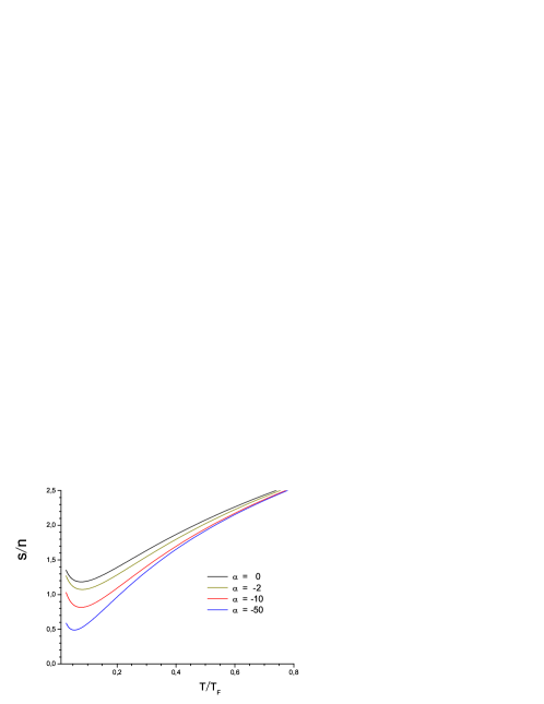
Figure 5: Entropy per particle as a function of $T/T_{F}$.

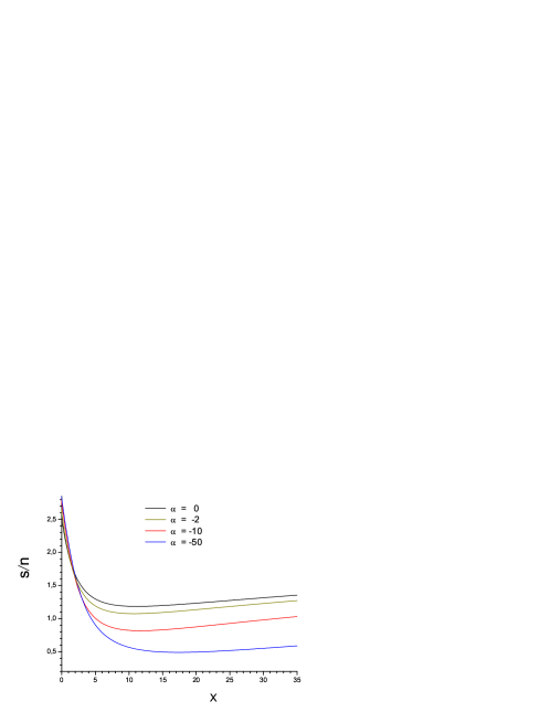
Figure 6: Entropy per particle as a function of $x=\mu/T$.

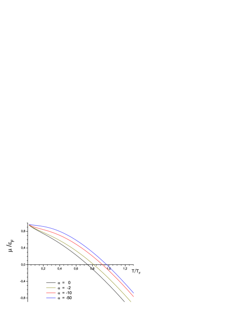
Figure 7: $\mu/\epsilon_{F}$ as a function of $T/T_{F}$.

As explained above, we use the entropy per particle plots to identify the critical point. One sees from Figure 5 that the entropy begins to increase as a function of temperature when the temperature is low enough, which is interpreted as being unphysical; it is actually ill defined below this temperature, i.e. there is no longer a solution $y$ to the integral equation. This change in behavior is also seen in Figure 6. For instance, in the unitary limit $\alpha=0^{-}$, the critical point is at $x_{c}\approx 11.$ which corresponds to $T/T_{c}\approx 0.08$. In Figure 8 we plot our results for $T_{c}/T_{F}$ as a function of $1/k_{F}a_{s}$. Our results are in rough agreement with the most recent Monte-Carlo results ming1 ; Proko ; bulga1 ; bulga2 . In the range $-0.5<1/k_{F}a_{s}<0$ the Monte-Carlo results are $0.08<T_{c}/T_{F}<0.15$, whereas we obtain $0.07<T_{c}/T_{F}<0.08$, which is on the low side.

Figure 8: $T_{c}/T_{F}$ as a function of $1/k_{F}a_{s}$ for fermions.

VII Conclusions

We have applied the S-matrix based formalism developed in PyeTon to bosons and fermions with arbitrary negative scattering length, extending the results in PyeTonUnitary2 at the unitary limit. We explored the virial expansion up to the fourth order within our approximation, confirming that $b_{2}$ for fermions is exactly correct, i.e. agrees with known results computed by different methods. We extended these calculations to bosons and both bosons and fermions to the other side of unitarity, that is, the upper branch. Our value for $b_{3}$ for fermions on the other hand, when compared with more accurate calculations and experiments, indicates the importance of the need to incorporate 3-body processes, and we hope to carry this out in the future based on the prescription described in PyeTon .

We applied the method as an exploratory tool for less-studied regimes. In particular, for bosons, assuming they can be meta-stable against mechanical collapse, we calculated $T_{c}$ for a strongly coupled Bose-Einstein condensation as a function of (negative) scattering length. We hope that our results in this case may be compared with other methods, or better, experiments, in the near future.

VIII Acknowledgments

We wish to thank Y. Castin, V. Gurarie, E. Mueller and F. Werner for discussions. This work is supported by the National Science Foundation under grant number NSF-PHY-0757868 and by FAPERJ (Fundação Carlos Chagas Filho de Amparo à Pesquisa do Estado do Rio de Janeiro) and CNPq (Conselho Nacional de Desenvolvimento Científico e Tecnológico).

IX Appendix A

For simplicity consider the bosonic case $s=+1$. By using $|\mathbf{k}-\mathbf{k}^{\prime}|=\sqrt{k^{2}+(k^{\prime})^{2}-2kk^{\prime}\cos\theta}\;,$ where $|\mathbf{k}|=k$, and integrating in spherical coordinates, one has:

$$y(\mathbf{k}) = 1-{4\beta\over m\pi}\int_{0}^{\infty}d\rho\,\rho^{2}{z\over e^{\beta\omega_{\mathbf{k}^{\prime}}}-zy(k^{\prime})}\int_{0}^{\pi}d\theta{\sin\theta\over\sqrt{k^{2}+\rho^{2}-2k\rho\cos\theta}}$$ (31)

$$\cdotp\;\arctan\left({mg_{R}\over 8\pi}\sqrt{k^{2}+\rho^{2}-2k\rho\cos\theta}\right)$$

$$= 1+{4\beta\over m\pi}\int_{0}^{\infty}d\rho\,\rho^{2}{z\over e^{\beta\omega_{\mathbf{k}^{\prime}}}-zy(k^{\prime})}\int_{1}^{-1}{dx\over\sqrt{a-bx}}$$

$$~{}~{}~{}~{}~{}\cdotp\;\arctan\left({mg_{R}\over 8\pi}\sqrt{a-bx}\right)\>,$$

where $\rho\equiv|\mathbf{k}^{\prime}|$, $a\equiv k^{2}+\rho^{2}\,$ , and $\>b\equiv 2k\rho\,$. In the third line above, the function $y(\mathbf{k})$ is considered to be spherically symmetric ($y(\mathbf{k})=y(k)$).

Evaluating the second integral

$$\int_{1}^{-1}{dx\over\sqrt{a-bx}}\arctan\left({mg_{R}\over 8\pi}\sqrt{a-bx}\right)$$

$$={1\over k\rho}\left[-(k+\rho)\arctan\left({mg_{R}\over 8\pi}(k+\rho)\right)+(k-\rho)\arctan\left({mg_{R}\over 8\pi}(k-\rho)\right)\right.$$

$$\qquad\;\left.+{4\pi\over mg_{R}}\log\left[{1+\left({mg_{R}\over 8\pi}\right)^{2}(k+\rho)^{2}\over 1+\left({mg_{R}\over 8\pi}\right)^{2}(k-\rho)^{2}}\right]\right]\>,$$

one obtains:

$$y(k) = 1+{4\beta\over m\pi}\int d\rho\,\rho{z\over e^{\beta\rho^{2}/2m}-zy(\rho)}\,{1\over k}\left\{{4\pi\over mg_{R}}\>\log\left[{\left({8\pi\over mg_{R}}\right)^{2}+(k+\rho)^{2}\over\left({8\pi\over mg_{R}}\right)^{2}+(k-\rho)^{2}}\right]\right.$$

$$\left.-(k+\rho)\arctan\left({mg_{R}\over 8\pi}(k+\rho)\right)+(k-\rho)\arctan\left({mg_{R}\over 8\pi}(k-\rho)\right)\right\}\,.$$

Rescaling $k\to\sqrt{2mT}k,\rho\to\sqrt{2mT}\rho$, and introducing $\alpha=\lambda_{T}/a_{s}$, one finds that the integral equation of $y(\kappa)$ can be written as in eq. (III).

The eq. (III) is valid for any value of $g_{R}$. As a consistency check, one can verify that in the unitary limit $g_{R}\>\rightarrow\>\pm\>\infty\,\Rightarrow\,\alpha\>\rightarrow\>0^{\pm}\>,$ one obtains

$$y(\kappa)=1\mp 4\int d\kappa^{\prime}{z\over e^{\kappa^{\prime}}-zy(\kappa^{\prime})}\left[\Theta(\kappa-\kappa^{\prime})\sqrt{{\kappa^{\prime}\over\kappa}}+\Theta(\kappa^{\prime}-\kappa)\right]\>$$ (32)

where $\kappa=k^{2}$, which is equivalent to expression (27) of PyeTonUnitary2 .

References

- (1) Y. Shin, C. Schunck, A. Schirotzek and W. Ketterle, Phase diagram of a two-component Fermi gas with resonant interactions, Nature 451 (2008) 689.
- (2) I. Bloch, J. Dalibard and W. Zwerger, Many-body physics with ultracold gases, Rev. Mod. Phys. 80 (2008) 885.
- (3) C. Chin, R. Grimm, P. Julienne and E. Tiesinga, Feshbach Resonances in Ultracold Gases, Rev. Mod. Phys. 82 (2010) 1225.
- (4) S. Nascimbène, N. Navon, K. J. Jiang, F. Chevy and C. Salomon, Exploring the thermodynamics of a universal Fermi gas, NATURE 463 (2010) 1057.
- (5) K. Van Houcke, F. Werner ,E. Kozik, N. Prokof ev, B. Svistunov, M.J.H. Ku, A.T.Sommer, L.W. Cheuk, A. Schirotzek, and M.W. Zwierlein, Feynman diagrams versus Fermi-gas Feynman emulator, Nature Physics (2012) doi:10.1038/nphys2273
- (6) M. Horikoshi, S. Nakajima, M. Ueda and T. Mukaiyama, Measurement of universal thermodynamic functions for a unitary Fermi gas, Science 327 (2010) 442.
- (7) A. Minguzzi, S. Succi, F. Toschi, M.P. Tosi and P. Vignolo, Numerical methods for atomic quantum gases with applications to Bose-Einstein condensates and to ultracold fermions, Phys. Reports 395 (2004) 223.
- (8) E. Burovski, N. Prokof’ev, B. Svistunov and M. Troyer, Critical temperature and thermodynamics of attractive fermions at unitarity, Phys. Rev. Lett 96 (2006) 160402.
- (9) A. Bulgac, J. E. Drut and P. Magierski, Quantum Monte Carlo Simulations of the BCS-BEC Crossover at Finite Temperature, Phys.Rev. A78 (2008) 023625.
- (10) P. Magierski, G. Wlazlowski, A. Bulgac and J.E. Drut, Finite-Temperature Pairing Gap of a Unitary Fermi Gas by Quantum Monte Carlo Calculations Phys. Rev. Lett. 103 (2009) 210403.
- (11) Y. Castin and F. Werner, The Unitary Gas and its Symmetry Properties, Springer Lecture Notes in Physics, “BEC-BCS Crossover and the Unitary Fermi Gas”, W. Zwerger, ed. [arXiv:1103.2851]
- (12) H. Hu, X.-J. Liu and P. D. Drummond, Universal thermodynamics of a strongly interacting Fermi gas: theory verses experiment, New J. of Phys. 12, 063038 (2010).
- (13) P. T. How and A. LeClair, Critical point of the two-dimensional Bose gas: an S-matrix approach, Nucl. Phys. B824 (2010) 415 [arXiv:0906.033]
- (14) C. N. Yang and C. P. Yang, Jour. Math. Phys. 10 (1969) 1115.
- (15) P.-T. How and A. LeClair, S-matrix approach to quantum gases in the unitary limit I: the two-dimensional case, J.Stat.Mech. (2010) P03025.
- (16) P.-T. How and A. LeClair, S-matrix approach to quantum gases in the unitary limit II: the three-dimensional case, J. Stat. Mech. (2010) P07001.
- (17) A. LeClair, On the viscosity-to-entropy density ratio for unitary Bose and Fermi gases, New J. of Phys. 13 (2011) 055015.
- (18) C. Cao, E. Elliot, J. Joseph, H. Wu, J. Petricka, T. Schäfer and J. E. Thomas, Universal Quantum Viscosity in a Unitary Fermi Gas, Science 331 (2011) 58.
- (19) W. Ketterle, private communication.
- (20) K. Dieckmann, C.A. Stan, S. Gupta, Z. Hadzibabic, C.H. Schunck, and W. Ketterle, Decay of an ultracold fermionic lithium gas near a Feshbach resonance, Phys. Rev. Lett. 89 (2002) 203201.
- (21) S. Jochim, M. Bartenstein, A. Altmeyer, G. Hendl, C. Chin, J.H. Denschlag and R. Grimm, Pure gas of optically trapped molecules created from fermionic atoms Phys. Rev. Lett. 91 (2003) 240402.
- (22) J. P. Gaebler, J. T. Stewart, T. E. Drake, D. S. Jin, A. Perali, P. Pieri and G. C. Strinati, Observation of pseudogap behaviour in a strongly interacting Fermi gas, Nature Physics 6 (2010) 569.
- (23) S. Tsuchiya, R. Watanabe, and Y. Ohashi, Single-particle properties and pseudogap effects in the BCS-BEC crossover regime of an ultracold Fermi gas above , Phys. Rev. A 80, 033613 (2009).
- (24) V. B. Shenoy and T.-L. Ho, Nature and Properties of a Repulsive Fermi Gas in the Upper Branch of the Energy Spectrum, Phys. Rev. Lett. 107 (2011) 210401.
- (25) Density and spin response of a strongly-interacting Fermi gas in the attractive and quasi-repulsive regime, F. Palestini, P. Pieri, G. C. Strinati, Phys. Rev. Lett. 108 (2012) 080401.
- (26) W. Li, T-L. Ho, Bose Gases Near Unitarity, arXiv:1201.1958v3 [cond-mat.quant-gas].
- (27) L. D. Landau and E. M. Lifshitz, Quantum Mechanics: Non-relativistic Theory, Pergamon, Oxford, 1977.
- (28) T. L. Ho and E. J. Mueller, High Temperature Expansion Applied to Fermions near Feshbach Resonance, Phys. Rev. Lett. 92 (2004) 160404.
- (29) A.J. Liu, H. Hu and P. D. Drummond, Virial expansion for a strongly correlated Fermi gas, Phys. Rev. Lett. 102 (2009) 160401.
- (30) X. Leyronas, Virial expansion with Feynman diagrams, Phys. Rev. A84 (2011) 053633.