Automated Synthesis of Dynamically Corrected Quantum Gates

Abstract

Dynamically corrected gates are extended to non-Markovian open quantum systems where limitations on the available controls and/or the presence of control noise make existing analytical approaches unfeasible. A computational framework for the synthesis of dynamically corrected gates is formalized that allows sensitivity against non-Markovian decoherence and control errors to be perturbatively minimized via numerical search, resulting in robust gate implementations. Explicit sequences for achieving universal high-fidelity control in a singlet-triplet spin qubit subject to realistic system and control constraint are provided, which simultaneously cancel to the leading order the dephasing due to non-Markovian nuclear-bath dynamics and voltage noise affecting the control fields. Substantially improved gate fidelities are predicted for current laboratory devices.

I Introduction

Achieving high-precision control over quantum dynamics in the presence of decoherence and operational errors is a fundamental goal across coherence-enabled quantum sciences and technologies. In particular, realizing a universal set of quantum gates with sufficiently low error rate is a prerequisite for fault-tolerant quantum computation Knill (2005). Open-loop control based on time-dependent modulation of the system dynamics has been extensively explored as a physical-layer error-control strategy to meet this challenge. Two main approaches have been pursued to date: on the one hand, if the underlying open-system relaxation dynamics is fully known, powerful variational techniques and/or numerical algorithms from optimal quantum control theory (OCT) may be invoked to optimize the target gate fidelity, see e.g. Tho ; Wha ; Clausen et al. (2010); Hwang and Goan (2012) for representative contributions. On the other hand, dynamically corrected gates (DCGs) dcg have been introduced having maximum design simplicity and portability in mind: close in spirit to well-established dynamical decoupling techniques for quantum state preservation in non-Markovian environments lvd , DCG sequences can achieve a substantially smaller net decoherence error than individual “primitive” gates by making minimal reference to the details of the system and control specifications. In principle, the use of recursive control design makes it possible for the final accuracy to be solely limited by the shortest achievable control time scale Khodjasteh et al. (2010). Remarkably, simple DCG constructions underly the fidelity improvement reported for spin-motional entangling gates in recent trapped-ion experiments Hay .

While obtaining a detailed quantitative characterization of the noise mechanisms to overcome is imperative to guarantee truly optimal control performance, this remains practically challenging for many open quantum systems of interest. In addition, current approaches for applying OCT methods to non-Markovian environments rely on obtaining suitable simplifications of the open-system equations of motion (e.g., via identification of a finite-dimensional Markovian embedding Tho or approximation through time-local coupled linear equations Hwang and Goan (2012)) – which may be technically challenging and/or involve non-generic assumptions. Since in DCG schemes the error cancellation is engineered at the level of the full system-plus-environment Hamiltonian evolution, two significant advantages arise: environment operators may be treated symbolically, avoiding the need for an explicit equation of motion for the reduced dynamics to be derived; in contrast to error-control approaches designed in terms of gate propagators (notably, fully compensating composite pulses for systematic control errors Levitt ; KenReview ), working at the Hamiltonian level allows to more directly relate to physical error mechanisms and operational constraints. Despite incorporating realistic requirements of finite maximum control rates and amplitudes, analytic DCG constructions nonetheless rely on the assumption that complete control over the target system can be afforded through a universal set of stretchable control Hamiltonians dcg . This requirement is typically too strong for laboratory settings where only a limited set of control Hamiltonians can be turned on/off with sufficient precision and speed, and universality also relies on internal always-on Hamiltonians. Furthermore, portability comes at the expenses of longer sequence durations, making DCGs more vulnerable to uncompensated Markovian decoherence mechanisms.

In this work, we introduce a control methodology that results in an automated recipe for synthesizing DCGs via numerical search. This is accomplished by relaxing the portability requirement and utilizing the full details of the control. While the resulting “automated DCGs” (aDCGs) are still synthesized without quantitative knowledge of the underlying error sources, they overcome the restrictive assumptions of analytical schemes and lead to drastically shorter sequences. As an additional key advantage, our Hamiltonian-engineering formulation lends itself naturally to incorporating robustness against multiple error sources, that can enter the controlled open-system Hamiltonian in either additive or multiplicative fashion. This allows for aDCGs to simultaneously cancel non-Markovian decoherence and control errors, as long as the combined effects remain perturbatively small.

We quantitatively demonstrate these advantages by focusing on a highly constrained control scenario – the two-electron singlet-triplet (S-T₀) spin qubit in GaAs quantum dots (QDs)Levy (2002). In spite of ground-breaking experimental advances Coh ; Hen ; Sch ; Dial , boosting single-qubit gate fidelities is imperative for further progress towards scalable quantum computation and is attracting intense theoretical effort Talk ; Mat ; Das . Recently introduced supcode composite-pulse sequences Das , for instance, are (analytically) designed to achieve insensitivity against decoherence induced by coupling to the surrounding nuclear-spin bath, however they do not incorporate robustness against voltage noise, which is an important limitation in experiments Dial . Here, we provide explicit aDCG sequences for high-fidelity universal control in S-T₀ qubits, which cancel the dominant decoherence and exchange-control errors, while respecting the stringent timing and pulsing constraints of realistic S-T₀ devices. The resulting sequences use a very small number of control variables and a fixed base pulse profile, which streamlines their experimental implementation. Up to two orders of magnitude improvement in gate fidelities are predicted for parameter regimes appropriate for current experimental conditions.

II Control-theoretic setting

We consider in general a $d$-dimensional target quantum system $S$ coupled to an environment (bath) $B$, whose total Hamiltonian $H$ on ${\cal H}_{S}\otimes{\cal H}_{B}$ reads

$$H = [H_{S}+H_{\text{ctrl},0}(t)]\otimes{\mathbb{I}}_{B}+H_{e},$$ (1)

$$H_{e} \equiv H_{e,\text{int}}+H_{e,\text{ctrl}}(t),$$

where ${\mathbb{I}}_{B(S)}$ denotes the identity operator on $B$($S$), $H_{S}$ accounts for the internal (“drift”) system’s evolution in the absence of control, and the time-dependent $H_{\text{ctrl},0}(t)$ represents the intended control Hamiltonian on $S$. The total “error Hamiltonian” $H_{e}$ encompasses the bath Hamiltonian, unwanted interactions with the bath, as well as deviations of the applied control Hamiltonian from $H_{\text{ctrl},0}(t)$, subject to the requirement that the underlying correlation times are sufficiently long. Formally, we require that $\|H_{e}\|\ll\|H(t)\|$, where $\|X\|$ is the operator norm of $X=X^{\dagger}$ (maximum absolute eigenvalue of $X$) lvd ; dcg . In order to “mark” the error sources, we characterize the strength of each independent contribution to $H_{e,\text{int}}$ in terms of dimensionless parameters $\{\delta_{\alpha}\}$, in such a way that, without loss of generality, we may express

$$H_{e,\text{int}}={\mathbb{I}}_{S}\otimes H_{B}+H_{SB}\equiv\sum_{\alpha}\delta_{\alpha}S_{\alpha}\otimes B_{\alpha},$$

with $S_{\alpha}$ being a Hermitian operator basis on ${\cal H}_{S}$ and $B_{\alpha}$ acting on ${\cal H}_{B}$, respectively, and the bath internal Hamiltonian $H_{B}\equiv\delta_{0}^{e}B_{0}$. We assume that the $B_{\alpha}$ are norm-bounded but otherwise quantitatively unspecified. In particular, if $B_{\alpha}$ are treated as scalars ($B_{\alpha}=\ell_{\alpha}{\mathbb{I}}_{B}$), we may formally recover the limit of a classical bath, whereby $B_{0}=0$ and the system Hamiltonian is effectively modified in a random (yet slowly time-dependent) fashion. Note that, as long as we are interested in canceling effects that are first order in the error sources, there is no distinction between the $B_{\alpha}$ being actual operators or scalars. Similarly, we characterize the independent error sources in $H_{\text{ctrl},0}(t)$ by letting

$$H_{e,\text{ctrl}}(t)=\sum_{\beta}\delta_{\beta}H_{\beta}(t)\otimes{\mathbb{I}}_{B},$$

where $H_{\beta}(t)$ are known system operators, while the parameters $\delta_{\beta}$ remain unspecified. For notational convenience, we shall label all the unknown parameters symbolically and collectively by $\delta\equiv\{\delta_{\alpha},\delta_{\beta}\}$.

In an ideal error-free scenario, $\delta=0$, the system evolves directly under the action of the control, in the presence of its internal drift Hamiltonian. We assume that in this limit, $S$ is completely controllable, that is, arbitrary unitary transformations on $S$ can be synthesized as “primitive gates” by suitably designing $H_{\text{ctrl},0}(t)$ in conjunction with $H_{S}$. As mentioned, we are particularly interested in the situation where the latter is essential for controllability to be achieved Remark . The available control resources may be specified by describing

$$H_{\text{ctrl},0}(t)=\sum_{a}c_{a}(t)H_{a}\otimes{\mathbb{I}}_{B},$$

in terms of the admissible (nominal) control inputs and Hamiltonians. Beside restrictions on the set of tunable Hamiltonians $H_{a}$, limited “pulse-shaping” capabilities will typically constrain the control inputs $c_{a}(t)$ as system-dependent features of the control hardware. For concreteness, we assume here that $H_{\text{ctrl},0}(t)$ is decomposed as a sequence of shape-constrained pulses applied back to back and also constrain pulse amplitudes $\{h_{i}\}$ and durations $\{\tau_{i}\}$ to technological limitations such as $h_{\text{min}}\leq h_{i}\leq h_{\text{max}},\tau_{\text{min}}\leq\tau_{i}\leq\tau_{\text{max}}$.

Ideally, if the target unitary gate is $Q$, the objective for gate synthesis is to devise a control Hamiltonian $H_{\text{ctrl},0}(t)$ such that (up to a phase),

$$Q={\cal T}\exp\Big{[}-i\int_{0}^{\tau}(H_{S}+H_{\text{ctrl},0}(s))\,ds\Big{]},$$ (2)

where ${\cal T}$ denotes time ordering and $\tau$ is the running time of the control. The ideal evolution naturally defines a toggling-frame unitary propagator given by

$$U_{Q}(t)={\cal T}\exp\Big{[}-i\int_{0}^{t}(H_{S}+H_{\text{ctrl},0}(s))\,ds\Big{]},$$ (3)

which traces a path from ${\mathbb{I}}_{S}$ to $Q$ over $\tau$. If $H_{e}\neq 0$, application of $H_{\text{ctrl},0}(t)$ over the same time interval results in a total propagator of the form

$$U^{(\delta)}_{Q[\tau]}\equiv U^{(0)}_{Q[\tau]}\exp(-iE_{Q[\tau]}^{(\delta)}),$$

where $U^{(0)}_{Q[\tau]}=Q$ and $E_{Q[\tau]}^{(\delta)}$ is an “error action” operator on ${\cal H}_{S}\otimes{\cal H}_{B}$ that isolates the effects of undesired terms in the evolution dcg :

$$\exp(-iE_{Q[\tau]}^{(\delta)})={\cal T}\exp\Big{[}-i\int_{0}^{\tau}U_{Q}(s)^{\dagger}H_{e}U_{Q}(s)\,ds\Big{]}.$$ (4)

The norm of the error action can be taken to quantify the error amplitude per gate (EPG) in the presence of $\delta$. The EPG in turn upper-bounds the fidelity loss between the ideal and actual evolution on $S$ once its “pure-bath” components are removed. More concretely, define

$$\text{mod}_{B}E\equiv E-\mathbb{I}_{S}\otimes\mbox{Tr}_{S}(E)/d,$$

that is, a projector that removes the pure-bath terms in $E$ (note that mod${}_{B}E=E$ if $E$ is a pure-system operator of the form $A\otimes{\mathbb{I}}_{B}$, as for a classical bath). Then the following (not tight) upper bound for the (Uhlman) fidelity loss holds independently of the initial states Lidar et al. (2008); Khodjasteh et al. (2010):

$$1-f_{U}\leq\|\text{mod}_{B}E_{Q[\tau]}^{(\delta)}\|.$$

Thus, reducing the EPG can be used as a proxy for reducing gate fidelity loss. While for a primitive gate implementation the EPG scales linearly with $\delta$, the goal of DCG synthesis is to perturbatively cancel the dependence on $\delta$ in $E_{Q[\tau]}^{(\delta)}$ up to a desired order of accuracy, to realize the gate in a manner that is as error free as possible as long as $\delta$ is small. For simplicity and immediate application, we focus here on first-order aDCG constructions, for which $\|\text{mod}_{B}E_{Q[\tau]}^{(\delta)}\|=O(\delta^{2})$.

III Synthesizing Dynamically Corrected Gates

III.1 Existential approach

Recall that two main requirements are required in first-order analytical DCG constructions dcg ; Khodjasteh et al. (2010): (i) primitive gate implementations of the generators of a “decoupling group” associated with the algebraic structure of EPGs and (ii) particular implementations of the target gate $Q$ (as $Q^{*}$) and the identity gate (as $I_{Q}$) as sequences of primitive gates such that $Q^{*}$ and $I_{Q}$ share the same first-order EPG, making them a “balance pair”. While (i) is provided by controllability and leads directly to a constructive procedure for correcting to the first-order the identity evolution, (ii) is essential for modifying this procedure in such a way that the net first-order error cancellation is maintained, but $Q$ is effected instead.

Generating balance pairs require further adjustment of gate control parameters to form a controllable relationship between EPGs of gate implementations, holding as an identity regardless of the value of $\delta$ (or $B_{\alpha}$). For example, in the absence of drift dynamics and control errors, such a controllable relationship can be engineered by “stretching” pulse profiles in time while the amplitudes are reduced proportionally, resulting in different realizations of the same target, with EPGs that scale linearly with the gate duration. Similarly, in the presence of a multiplicative control error, primitive gates with physically equivalent (modulo $2\pi$) angles of rotation result in different EPGs (note that similar geometric ideas are used in designing composite pulses KenReview ). We argue next that knowing the control description and marking the error sources $\{\delta_{j}\}$ does still lead to (ii) as long as control constraints allow us to tap into a continuum of different gate implementations.

The multitude of pathways for realizing a primitive gate $Q$ increases with gate duration/subsegments as a result of availability of more control choices and ultimately a simpler control landscape Moo . Assume that (A1) such primitive implementations may be parametrized as $Q[\tau]$. We aim to show that a balance pair or, alternatively, a direct cancellation of the EPG of $Q$ may be found. The gist of our argument is most easily given for a single qubit, with the Pauli operators chosen as the operator basis $\{S_{\alpha}\}$ for error expansion. Using the fact that the interactions among different error sources can be ignored up to the first order, the basic idea is to start with the first error source, $\delta_{1}$, and then use the resulting gates recursively for the next error source until all error sources are exhausted. Ignoring error sources other than $\delta_{1}$, let us thus expand $E^{(\delta_{1})}_{Q[\tau]}=\delta_{1}\sum_{\alpha}e_{Q[\tau],\alpha}S_{\alpha}\otimes B_{1}$.

Assume in addition that (A2), as a function of the parameter $\tau$, the range of the real-valued functions $e_{Q[\tau],\alpha}$ extends to infinity in positive or negative directions. Consider now “projection blocks” composed of two Pauli gates applied back to back, that is,

$$P_{\alpha}[\tau_{\alpha}]\equiv S_{\alpha}[\tau_{\alpha}]S_{\alpha}[\tau_{\alpha}],$$

with a corresponding EPG given by $2\delta_{1}e_{S_{\alpha}[\tau_{\alpha}],\alpha}S_{\alpha}\otimes B_{1}$, which is purely along $S_{\alpha}$. By virtue of (a2), we can find a continuum of $(\tau,\tau_{\alpha})$ pairs such that $2e_{S_{\alpha}[\tau_{\alpha}],\alpha}=\pm e_{Q[\tau],\alpha}$ for all Pauli directions $\alpha$, meaning that we may reproduce each error component in $E^{(\delta_{1})}_{Q[\tau]}$ up to a sign. Those Pauli components $\alpha_{-}$ that reproduce error with a negative sign are combined in sequence with $Q[\tau]$ to form a longer gate

$$Q^{*}=Q[\tau]\prod_{\alpha_{-}}\!P_{\alpha_{-}}[\tau_{\alpha_{-}}].$$

If all Pauli components can be matched with negative signs, the resulting gate will cancel all error components and a DCG construction is provided by $Q^{*}$. Otherwise, the Pauli components ${\alpha_{+}}$ that are matched with positive sign, are combined to produce an identity gate,

$$I_{Q}=\prod_{\alpha_{+}}\!P_{\alpha_{+}}[\tau_{\alpha_{+}}],$$

that matches the error of $Q^{*}$. Hence, $(Q^{*},I_{Q})$ form a balance pair and can be used to produce a continuum of constructions of a DCG gate $Q^{(1)}[\tau]$ that cancel the error source $\delta_{1}$. Provided that the assumption (A2) remains valid for this new composite constructions, we can repeat the procedure to remove the other error sources.

We remark that assumption (A2) essentially implies that the domain of the errors as a function of implementation parameters for a fixed unitary gate is not compact, so that arbitrary magnitudes of each error component can be sampled by appropriately choosing the implementation parameters. Such arbitrary large domains need not not exist in the primitive gate implementations (naturally or due to constraints), or only discrete error values may be reachable. Nonetheless, we may still enlarge the accessible range of errors for the target gate $Q$ by attaching a continuously parametrized family of identity gates. Universal controllability of the system implies that not only any gate $U$ but also its inverse $U^{-1}$ may be reached. Implementing $U$, followed by its inverse $U^{-1}$, produces an implementation of the identity $I_{U}$ “parametrized” by the original gate $U$. In the absence of degeneracies (relationships between the errors that could be used separately to provide a balance pair), the EPG associated with $E_{U}$ has then a continuos domain. Clearly, applying $I_{U}$ followed by the target gate $Q$ still realizes the gate $Q$ but the resulting EPG is now given by $E_{Q}+E_{I_{U}}$, which is parametrized by $U$. By applying sufficiently many copies of $I_{U}$ before applying $Q$, the error can be extended to arbitrary large domains as desired.

III.2 aDCGs: Computational Approach

The aDCG sequences generated by following the above existential argument tend to be far too long and complex to be useful in realistic control scenarios. Also note that in principle, the construction of single- or two-qubit DCGs in $n$-qubit registers may be handled similarly by using multi-qubit Pauli operators as a basis for EPG expansion and for building projection blocks. However, the sequence complexity tends in this case to also grow exponentially with $n$ Khodjasteh et al. (2010), making the need for more efficient synthesis procedures even more essential. Just as complete controllability provides an existential foundation to numerical OCT approaches for unitary gate synthesis when $H_{e}=0$ Mat , our argument legitimates a numerical search for aDCGs in the presence of $H_{e}$. Since the objectives of gate realization and perturbative error cancellation are not inherently competing, the numerical search can be described as multi-objective minimization problem, as we detail next.

Let the nominal control Hamiltonian $H_{\text{ctrl},0}(t)$ be parametrized in terms of control variables $\{x_{i}\}$ and define objective functions as follows:

$$F(\{x_{i}\}) = \text{dist}(U_{Q[\tau]}^{(\delta=0)},Q),$$ (5)

$$B_{j}G_{j}(\{x_{i}\}) = \|\partial\,\text{mod}_{B}E_{Q[\tau]}^{(\delta)}/\partial\delta_{j}\|_{\delta=0},$$ (6)

where $j$ labels independent error sources and $B_{j}$ symbolically denotes bath operators that mark error sources in $H_{e,\text{int}}$ (recall that $B_{j}={\mathbb{I}}_{B}$ for control error sources) to ensure that $F$ and $G_{j}$ only depend on the known quantities $x_{i}$. Minimizing only the first objective, $F=0$, corresponds to achieving exact ideal primitive gate synthesis, Eq. (2). As an appropriate distance measure for unitary operators in Eq. (5), we use

$$\text{dist}(U,V)=[1-|\text{Tr}(U^{\dagger}V)|/d]^{1/2},$$ (7)

which is a standard phase-invariant choice Mat . Minimizing the objectives in Eq. (6) corresponds to first-order sensitivity minimization. Thus, solving for $F=0=G_{j},\forall j$, results in an implementation of $Q$ that is insensitive to the perturbative parameters $\delta_{j}$, yielding a robust control solution as long as $\delta_{j}$ is small.

Evaluating $G_{j}$ apparently requires solving the full time-dependent system-plus-bath Schrödinger equation parametrized by the controllable pulse shapes. In fact, once the error sources (including bath operators) are treated as first-order symbolic variables, $G_{j}$ can be evaluated by effectively solving the Schrödinger equation on the system only, in order to determine the appropriate toggling-frame propagator, Eq. (3), and then evaluate the required error action, Eq. (4), by invoking a Magnus expansion dcg . Specifically, if the control variables $x_{i}\equiv\{(\tau_{i},h_{i})\}$, the sequence propagator reads

$$U_{Q[\tau]}^{(\delta)}\equiv U_{x_{n}}^{(\delta)}(\tau_{n})\cdots U_{x_{1}}^{(\delta)}(\tau_{1}),$$

where $\tau=\sum_{i}\tau_{i}$ and $U_{x_{i}}^{(\delta)}(s)$ is the $i$-th pulse propagator corresponding to the variable $x_{i}$ at time $s$, with its associated first-order error action,

$$E_{U_{x_{i}}}^{(\delta)}=\int_{0}^{\tau_{i}}U_{x_{i}}^{(0)}(s)^{\dagger}H_{e}U_{x_{i}}^{(0)}(s)ds.$$

To the first order in $\delta$, the total EPG is in turn given by

$$E_{Q[\tau]}^{(\delta)}=\sum_{i}V_{i}^{\dagger}E_{U_{x_{i}}}^{(\delta)}V_{i},$$

where $V_{i}\equiv U_{x_{i-1}}^{(0)}\cdots U_{x_{1}}^{(0)}$ denote the “partial” product of gate propagators up to and excluding the $i$-the gate dcg . While, as noted, for a first-order aDCG the resulting accuracy $\text{mod}_{B}E_{Q[\tau]}^{(\delta)}\|=O(\delta^{2})$, a more quantitative estimate of the actual conditions of applicability requires estimating the dominant uncorrected second-order errors. Technically, this can be carried out by means of standard algebraic techniques however is not straightforward ser and beyond our present scope. Instead, we focus in what follows on addressing the construction and performance of first-order aDCGs in concrete illustrative settings.

IV Application to singlet-triplet qubits

Consider first the following single-qubit specialization of Eq. (1):

$$H = \frac{1}{2}\Big{[}{B}\sigma_{x}+J_{0}(t)\sigma_{z}\Big{]}\otimes{\mathbb{I}}_{B}+H_{e},$$ (8)

$$H_{e} = {\mathbb{I}}_{S}\otimes\delta_{0}B_{0}+\sigma_{x}\otimes\delta_{1}B_{x}+J_{0}(t)\delta_{2}\sigma_{z},$$

where the operator-valued $\delta_{1}B_{x}$ and the system drift $B$ couple to the system along $\sigma_{x}$ and the nominal control $J_{0}(t)$ and a multiplicative error $\delta_{2}$ couple along $\sigma_{z}$. Although explicitly included, the bath internal Hamiltonian does not play a role in the first-order removal of decoherence and is automatically accounted for in mod_B. On the other hand, the drift term $B$ is essential for complete controllability and analytical DCG constructions are not viable even in the limit $\delta_{2}\rightarrow 0$. Thus, the need to effectively address both noise sources $\delta_{1},\delta_{2}$ for a generic operating point $B$ mandates the use of aDCGs.

While useful as a template for single-axis control scenarios in the presence of internal drift and dephasing, a semi-classical version the above model is relevant, in particular, to describe a universally controllable S-T₀ qubit. In this case, the logical qubit subspace is spanned by $\{|S\rangle,|T_{0}\rangle\}$, the singlet and triplet states of two electrons on separate QDs tay ; Hen ; Sch ; Das and, provided that the number of bath nuclear spins is sufficiently large tay , the following simpler Hamiltonian is appropriate and widely used for this system Mat ; Das :

$$H=\frac{1}{2}\Big{[}{B+\delta B(t)}\Big{]}\sigma_{x}+\frac{1}{2}{J(t)}\sigma_{z}.$$ (9)

Physically, the drift term $B$ is a known static magnetic field gradient between the two QDs that includes an Overhauser field from the nuclear spin bath, $\delta B(t)$ (corresponding to $2\delta_{1}B_{x}$) accounts for random fluctuations of $B$ due to coupling to nuclear flip-flop processes Cywiński et al. (2009), and $J(t)$ is the exchange splitting. In practice, $J(t)$ is tuned by control of an electrostatic gate voltage Hen , and voltage fluctuations due to charge noise result in a noisy control Hamiltonian of the form $J(t)=J_{0}(t)(1+\delta J(t))$, where $\delta J(t)$ thus corresponds to $2\delta_{2}$. We assume that both noise sources may be treated as Gaussian quasi-static processes, with their “run-to-run” distribution being characterized by standard deviations $\sigma_{\delta B}$ and $\sigma_{\delta J}$. While in practice the noise is not completely static, we expect our considerations to remain valid as long as high-frequency noise components decay sufficiently fast and the resulting aDCGs are short relative to time scales over which white charge noise may become important. Phenomenologically, the dephasing induced by the fluctuating Overhauser field is consistent with a power-law noise spectrum of the form $S(\omega)\sim\omega^{-2}$ over a wide spectral range Mike . Likewise, recent experiments indicate that voltage noise also arises overwhelmingly due to low-frequency components with an approximate $1/f$ decay at low operating temperatures Dial . From experimentally measured values of $T_{2}^{\star}$, we use here $\sigma_{\delta B/(2\pi)}\lesssim 0.15$ MHz Coh and $\sigma_{\delta J}\lesssim 1/50$ jno .

In constructing aDCGs, we shall choose values of the internal drift ($B$) and of the nominal control field ($J_{0}(t)$) appropriate for the QD setting of Eq. (9). We stress, however, that the same solution is found from (and applies to) the fully quantum model Hamiltonian of Eq. (8). In practice, the drift term $B$ can be set to a fixed value $B/2\pi\in[0.03,0.2]\,$GHz, which we choose at $0.1\,$GHz bopt . The control field $J_{0}(t)/2\pi$ is taken to be positive and smaller than $J_{\text{max}}=0.3\,$GHz. We recognize the finite rise, delay, and drop times associated with pulse generators by fixing a pulse profile. Thus, during each pulse, with time $t^{\prime}$ measured from the pulse start, the control function $J_{0}(t^{\prime})$ is given by $h_{i}c(t^{\prime}/\tau_{i})$, where $c(x)$ is the pulse shape function. We digitize the pulse shape function for numerical evaluation. In contrast to merely bounding the pulse times and allowing pulse durations as extra control variables, we enforce the pulse durations to be fixed at $\tau_{i}\equiv\tau=3\,$ns, that is compatible with the currently most widespread pulse generators temporal resolution of $0.83\,$ns. The search space of the pulse amplitude control variables is thus given by $x_{i}=h_{i}$. While removing $\tau_{i}$ from the control variables results in more severe constraints, it also corresponds to a reduction of the search space. We verified that all of our results were reproduced with variable but lower-bounded pulse widths as well. The objective functions $F$, $G_{1}$ and $G_{2}$ are computed explicitly in terms of each constituting pulse parameter $h_{i}$ according to the general procedure described in Sec. III.B.

For the resulting multi-objective minimization, we introduce numerical weight factors $\lambda_{1}$ and $\lambda_{2}$ and form a single objective function

$$O(\{h_{i}\})\equiv F+\lambda_{1}G_{1}+\lambda_{2}G_{2}.$$

Choosing small values of $\lambda_{i}$ ($=10^{-5}$) work best in directing the search from solutions that synthesized the target gate only at ($F=0$) first, and then towards the error-corrected solution $F=0,G_{1}=0=G_{2}$. Motivated by our existential argument, the intuition is to avoid the local minima associated with multiple objectives and focus on a single objective which, once realized, will give weight to the other objectives iteratively. We solve each aDCG search problem using off-the-shelf (Matlab’s fmincon function) search routine (within minutes), with the default choice for solving constrained nonlinear optimization without specifying a precalculated gradient or Hessian. We start the search with a small number of pulses, $n$, which is then incremented until the minimal value of the objective function comes close to the machine precision ($\approx 10^{-16}$). Fig. 1 (top) depicts the synthesized control profiles for a universal set of single-qubit aDCGs.

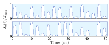
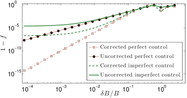
Figure 1: (Color online) Upper panel: aDCG control profiles for $\exp(-i\pi\sigma_{z}/8)$ (top) and the Hadamard gate (bottom). Lower panel: Fidelity loss for uncorrected vs. corrected gates, evaluated as 1$-f=\text{dist}(U_{Q}^{(\delta B,\delta J)},Q)^{2}$ [Eq. (7)], for $Q=\exp(-i\pi\sigma_{z}/8)$ as a function of relative magnetic field gradient error $\delta B/B$ ($B/(2\pi)=0.1\,$GHz). $\delta J=0$ corresponds to perfect exchange control, whilst $\delta J=0.01$ is close to current realistic levels. The fact that $\delta J=0.01$ is fixed is responsible for the eventual performance plateaux where the latter dominates over $\delta B$ effects. Nevertheless, the aDCG advantage is always maintained.

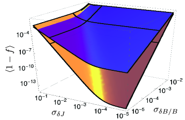
Figure 2: (Color online) Ensemble averaged fidelity loss as a function of relative magnetic field-gradient and exchange-control noise for uncorrected (top, dark) vs. corrected (bottom, light) implementation of $Q=\exp(-i\pi\sigma_{z}/8)$. The solid (black) lines on each surface correspond to typical values $\sigma_{\delta J}\approx 0.02$ and $\sigma_{\delta B/B}\approx 10^{-3}$ for current S-T₀ devices.

Once aDCG sequences are found, evaluating their effectiveness for the S-T₀ qubit can take direct advantage of the effectively closed-system nature of the model Hamiltonian in Eq. (9), thus avoiding the need of explicit spin-bath simulations and quantum process tomography. Fig. 1 (bottom) depicts the fidelity loss for an uncorrected ($n=3$ pulses, obtained through the same numerical procedure with $\lambda_{1}=\lambda_{2}=0$) vs. corrected implementation ($n=17$ pulses). The higher slope of the fidelity loss as a function of $\delta B$ when $\delta J=0$ is the signature of a perturbative error cancellation and the aDCG advantage is maintained even with $\delta J>0$, implying robustness with respect to both error types.

In order to make contact with experimentally relevant ensemble-averaged fidelities, we further evaluate the average of single-run fidelities $f(\delta B,\delta J)$ with respect to noise realizations, by assuming that $\delta B$ and $\delta J$ are independent and normally distributed random variables with variance $\sigma^{2}_{\delta B}$ and $\sigma^{2}_{\delta J}$. The results are summarized in Fig. 2. Both noise sources adversely impact the expected gate fidelity but aDCGs are far less affected, resulting in robust gates roughly as long as $\sigma_{\delta B/B}+\sigma_{\delta J}\lessapprox 0.1$.

V Conclusion

Our procedure can be interpreted as a automated gate compiler which incorporates detailed information about the controllable parameters and their range of operations, along with qualitative information about the error sources affecting the evolution. Compared to mere (primitive) gate synthesis, the resulting increase in complexity scales proportionally to the number of error sources. Our approach applies to any Hamiltonian control setting, and for weak enough error sources, even higher-order cancellation can be achieved in principle.

Thanks to the slow dynamics of the nuclear spin bath and fast control pulses available, electron spin qubits provide an ideal experimental testbed for validating our approach. While additional experimental details may be captured in more sophisticated ways, we believe that our framework is general and flexible enough for its effectiveness not to be compromised. In particular, further analysis is needed to quantify the effect of white electrical noise on aDCG sequences, as well as to possibly minimize its influence by penalizing large values of the exchange splitting in the numerical search. It is thus our hope that significantly improved single-gate fidelities will be achievable in S-T₀ qubits by aDCG sequences that operate under realistic noise levels and control limitations.

References

- Knill (2005) E. Knill, Nature 434, 39 (2005).
- (2) Khaneja et al., J. Magn. Res. 172, 296 (2005); T. Schulte-Herbrg̈gen et al., J. Phys. B 44, 154013 (2011).
- (3) M. Möttönen et al., Phys. Rev. A 73, 022332 (2006).
- Clausen et al. (2010) J. Clausen, G. Bensky, and G. Kurizki, Phys. Rev. Lett. 104, 040401 (2010).
- Hwang and Goan (2012) B. Hwang and H.-S. Goan, Phys. Rev. A 85, 032321 (2012).
- (6) K. Khodjasteh and L. Viola, Phys. Rev. Lett. 102, 080501 (2009); Phys. Rev. A 80, 032314 (2009).
- (7) L. Viola, E. Knill, and S. Lloyd, Phys. Rev. Lett. 33, 2417 (1999); L. Viola and E. Knill, ibid. 90, 037901 (2003).
- Khodjasteh et al. (2010) K. Khodjasteh, D. A. Lidar, and L. Viola, Phys. Rev. Lett. 104, 090501 (2010).
- (9) D. Hayes et al., Phys. Rev Lett. 109, 020503 (2012). See also D. Hayes et al., Phys. Rev. A 84, 062323 (2011).
- (10) M. Levitt, Progr. Nucl. Magn. Res. Spectr. 18, 61 (1986).
- (11) J. T. Merrill and K. R. Brown, arXiv:1203.6392.
- Levy (2002) J. Levy, Phys. Rev. Lett. 89, 147902 (2002).
- (13) J. R. Petta et al., Science 309, 2180 (2005); H. Bluhm et al., Phys. Rev. Lett. 105, 216803 (2010).
- (14) S. Foletti et al., Nature Phys. 5, 903 (2009).
- (15) M. D. Shulman et al., Science 336, 202 (2012).
- (16) O. E. Dial et al., arXiv:1208.2023.
- (17) Preliminary results were reported by L. Viola, “Towards optimal constructions of dynamically corrected gates,” Invited Talk at QEC 2011, available online at qserver.usc.edu/qec11/slides/Viola_QEC11.pdf.
- (18) M. D. Grace et al., Phys. Rev. A 85, 052313 (2012).
- (19) X. Wang et al., Nature Commun. 3, 997 (2012).
- (20) If universal control and sufficiently fast dynamical decoupling pulses are available, alternative strategies are possible for protecting quantum gates, most simply by embedding the desired gate into the initial or/and final free-evolution of a decoupling cycle, following ideas of L. Viola, S. Lloyd, and E. Knill, Phys. Rev. Lett. 83, 4888 (1999). A recent experimental implementation for a single solid-state qubit that also incorporates robustness against amplitude control errors was reported by A. M. Souza, G. A. Álvarez, and D. Suter, arXiv:1206.2933.
- Lidar et al. (2008) D. A. Lidar, P. Zanardi, and K. Khodjasteh, Phys. Rev. A 78, 012308 (2008).
- (22) K. W. Moore et al., arXiv:1112.0333.
- (23) Higher order terms need more work as the (commutatively built) products of do not form a basis for expansion of the error action operator, used to define . A so-called Hall basis can be used for expanding the latter in terms of algebraically free operator elements of a given perturbation order. See e.g. C. Reutenauer, Free Lie Algebras, Oxford University Press, USA (1993).
- (24) J. M. Taylor et al., Phys. Rev. B 76, 035315 (2007).
- Cywiński et al. (2009) L. Cywiński, W. M. Witzel, and S. D. Sarma, Phys. Rev. Lett. 102, 057601 (2009).
- (26) M. J. Biercuk and H. Bluhm, Phys. Rev. B 83, 235316 (2011).
- (27) This corresponds to ns for noise and about 11 coherent oscillations within for .
- (28) Changing the choice of the drift may change the solutions considerably, for instance, having removes controllability altogether. Note also that instead of fixing , we could in principle consider optimizing its value to be fixed across a set of desired gates.