Coherent Pattern Prediction in Swarms of Delay-Coupled Agents

Abstract

We consider a general swarm model of self-propelling agents interacting through a pairwise potential in the presence of noise and communication time delay. Previous work [Phys. Rev. E 77, 035203(R) (2008)] has shown that a communication time delay in the swarm induces a pattern bifurcation that depends on the size of the coupling amplitude. We extend these results by completely unfolding the bifurcation structure of the mean field approximation. Our analysis reveals a direct correspondence between the different dynamical behaviors found in different regions of the coupling-time delay plane with the different classes of simulated coherent swarm patterns. We derive the spatio-temporal scales of the swarm structures, and also demonstrate how the complicated interplay of coupling strength, time delay, noise intensity, and choice of initial conditions can affect the swarm. In particular, our studies show that for sufficiently large values of the coupling strength and/or the time delay, there is a noise intensity threshold that forces a transition of the swarm from a misaligned state into an aligned state. We show that this alignment transition exhibits hysteresis when the noise intensity is taken to be time dependent.

I Introduction

The rich dynamic behavior of interacting multi-agent, or particle, systems has been the focus of numerous recent studies. These multi-particle systems are capable of self-organization, as shown by the various coherent conformations with complex structure that they generate, even when the interactions are short range and in the absence of a leader agent. The study of these ‘swarming’ or ‘herding’ systems has had many interesting biological applications which have resulted in a better understanding of the spatio-temporal patterns formed by bacterial colonies, fish, birds, locusts, ants, pedestrians, etc. [1, 2, 3, 4, 5, 6, 7]. The mathematical study of these swarming systems is also helpful in the understanding of oscillator synchronization, as in the neural phenomenon of central pattern generators [8]. The results of these studies have impacted and have been successfully applied in the design of systems of autonomous, inter-communicating robotic systems [9, 10, 11, 12], as well as mobile sensor networks [13].

It is possible to design swarming models for robotic motion planning, consensus and cooperative control, and spatio-temporal formation. Pairwise potentials for individual agents can be straightforwardly ported onto autonomous vehicles. Furthermore, these pairwise interactions can be used in conjunction with simple scalable algorithms to achieve multi-vehicle cooperative motion [14]. Specific goals include: obstacle avoidance [11], boundary tracking [15], environmental sensing [13, 16] and decentralized target tracking [17].

An important problem is that of environmental consensus estimation. Here, the individuals of the swarm communicate with each other through a network to achieve asymptotically synchronous information about their environment [13]. Recently, consensus was extended to include time delayed communication among agents [18].

Task allocation is another problem of interest involving robotic swarms. The objective is to reallocate swarm robots to perform a set of tasks in parallel and independently of one another in an optimal way. In order to make task reallocation more realistic it is possible to consider a time delay that arises from the amount of time required to switch between tasks [19].

Regardless of the design objective of a robotic swarm system, a comprehensive theoretical analysis of the model must be performed in order to achieve successful algorithm design.

Many different mathematical approaches have been utilized to study aggregating agent systems. Some of these studies have treated the problem at a single-individual level, using ordinary differential equations (ODEs) or delay differential equations (DDEs) to describe their trajectories [20, 21, 22, 10]. An alternative method has been proposed by other researchers and consists of using continuum models that consider averaged velocity and agent density fields that satisfy partial differential equations (PDEs) [2, 3, 5, 6]. In addition, authors also have studied the effects of noise on the swarm’s behavior and have shown the existence of noise-induced transitions [23, 25]. The study of these systems has been enriched by tools from statistical physics since both first and second order phase transitions have been found in the formation of coherent states [28].

An additional effect that has recently been considered is that of communication time delays between robots. Time delay models are common in many areas of mathematical biology including population dynamics, neural networks, blood cell maturation, virus dynamics and genetic networks [29, 30, 31, 32, 33, 34, 35, 36, 37]. In the context of swarming agents, it has been shown that the introduction of a communication time delay may induce transitions between different coherent states in a manner which depends on the coupling strength between agents and the noise intensity [25]. Thus far, most of the work has concentrated on the case of uniform time delays among agents [26]. However, the practical engineering of multi-agent systems requires researchers to consider the case in which time delays may vary due to data processing times, problems in inter-agent communication, etc. The case of differing (and even time-vary ing) time delays between agents may be treated similarly to the case of a single delay by using a data buffer [27].

In this work, we carry out a detailed study of the bifurcation structure of the mean field approximation used in [25] and investigate how the bifurcations in the system are modified in the presence of noise. Section II contains the swarm model, while Sec. III contains the derivation of the mean field approximation. The bifurcation analysis of the mean field equation can be found in Sec. IV, and Sec. V provides a comparison of the mean field analysis with the nonlinear governing equations. In Sec. VI, we describe the effects of noise on the swarm, and the conclusions are contained in Sec. VII.

II Swarm Model

We consider a two-dimensional (2D) swarm that consists of $N$ identical self-propelling individuals of unit mass that are mutually attracted to one another in a symmetric fashion. Hence, the coupling of the agents occurs via a fully connected graph. In addition, we consider the case in which the individuals that comprise the swarm are communicating with each other in a stochastic environment. Because of the finite communication times between individuals, there is a time delay between interactions. Assuming that the communication time between agents is constant and equal to $\tau>0$, the swarm dynamics is described by the following governing equations:

$$\dot{\mathbf{r}}_{i}= \mathbf{v}_{i},$$ (1a)

$$\dot{\mathbf{v}}_{i}= \left(1-|\mathbf{v}_{i}|^{2}\right)\mathbf{v}_{i}-\frac{a}{N}\mathop{\sum_{j=1}^{N}}_{i\neq j}(\mathbf{r}_{i}(t)-\mathbf{r}_{j}(t-\tau))+\boldsymbol{\eta}_{i}(t),$$ (1b)

for $i=1,2\ldots,N$. The terms $\mathbf{r}_{i}$ and $\mathbf{v}_{i}$ respectively represent the 2D position and velocity of the $i$-th agent at time $t$. The strength of the attraction is measured by the coupling constant $a>0$. The self-propulsion and frictional drag forces on each agent is given by the term $\left(1-|\mathbf{v}_{i}|^{2}\right)\mathbf{v}_{i}$. Therefore, in the absence of coupling, agents tend to move on a straight line with unit speed $|\mathbf{v}_{i}|=1$ as time goes to infinity. The term $\boldsymbol{\eta}_{i}(t)=(\eta_{i}^{(1)},\eta_{i}^{(2)})$ is a 2D vector of stochastic white noise with intensity equal to $D$ such that $\langle\eta_{i}^{(\ell)}(t)\rangle=0$ and $\langle\eta_{i}^{(\ell)}(t)\eta_{j}^{(k)}(t^{\prime})\rangle=2D\delta(t-t^{\prime})\delta_{ij}\delta_{\ell k}$ for $i,j=1,2,\ldots N$ and $\ell,k=1,2$. It is the main objective of this work to identify the possible swarm behaviors for different values of $a$ and $\tau$.

The coupling between individuals arises from a time delayed, spring-like potential. Hence, our equations of motion may be considered to be the first term in a Taylor expansion of other more general time delayed potential functions about an equilibrium point.

III Mean Field Approximation

We can investigate the stability of the swarm system by deriving a mean field approximation of the system. The derivation involves the consideration of agent coordinates relative to the center of mass and the elimination of the noise terms. The center of mass of the swarming system is given by

$$\mathbf{R}(t)=\frac{1}{N}\sum_{i=1}^{N}\mathbf{r}_{i}(t).$$ (2)

The position of each individual can be decomposed into

$$\mathbf{r}_{i}=\mathbf{R}+\delta\mathbf{r}_{i},\qquad i=1,2\ldots,N,$$ (3)

where $\delta\mathbf{r}_{i}$ is the vector from the center of mass to particle $i$ and

$$\sum_{i=1}^{N}\delta\mathbf{r}_{i}(t)=0.$$ (4)

We substitute the ansatz given by Eq. (3) into the second order system that is equivalent to Eqs. (1a)-(1b) with $D=0$. After simplification, one obtains

$$\ddot{\mathbf{R}}+\delta\ddot{\mathbf{r}}_{i}= \left(1-|\dot{\mathbf{R}}|^{2}-2\dot{\mathbf{R}}\cdot\delta\dot{\mathbf{r}}_{i}-|\delta\dot{\mathbf{r}}_{i}|^{2}\right)(\dot{\mathbf{R}}+\delta\dot{\mathbf{r}_{i}})$$

$$-\frac{a(N-1)}{N}\bigg{(}\mathbf{R}(t)-\mathbf{R}(t-\tau)+\delta\mathbf{r}_{i}(t)\bigg{)}$$

$$-\frac{a}{N}\delta\mathbf{r}_{i}(t-\tau),$$ (5)

where we used the fact that Eq. (4) can be written as

$$\delta\mathbf{r}_{i}(t-\tau)=-\mathop{\sum\limits_{j=1}^{N}}\limits_{i\neq j}\delta\mathbf{r}_{j}(t-\tau).$$ (6)

Summing Eq. (III) over $i$ and using Eq. (4), we find

$$\ddot{\mathbf{R}}= \left(1-|\dot{\mathbf{R}}|^{2}-\frac{1}{N}\sum_{i=1}^{N}|\delta\dot{\mathbf{r}}_{i}|^{2}\right)\dot{\mathbf{R}}$$

$$-\frac{1}{N}\sum_{i=1}^{N}\left(2\dot{\mathbf{R}}\cdot\delta\dot{\mathbf{r}}_{i}+|\delta\dot{\mathbf{r}}_{i}|^{2}\right)\delta\dot{\mathbf{r}_{i}}$$

$$-a\frac{N-1}{N}\left(\mathbf{R}(t)-\mathbf{R}(t-\tau)\right).$$ (7)

By inserting Eq. (III) into Eq. (III) it is possible to find the following equation for $\delta\ddot{\mathbf{r}}_{i}$:

$$\delta\ddot{\mathbf{r}}_{i}= \left(\frac{1}{N}\sum_{j=1}^{N}|\delta\dot{\mathbf{r}}_{j}|^{2}-2\dot{\mathbf{R}}\cdot\delta\dot{\mathbf{r}}_{i}-|\delta\dot{\mathbf{r}}_{i}|^{2}\right)\dot{\mathbf{R}}$$

$$+\left(1-|\dot{\mathbf{R}}|^{2}-2\dot{\mathbf{R}}\cdot\delta\dot{\mathbf{r}}_{i}-|\delta\dot{\mathbf{r}}_{i}|^{2}\right)\delta\dot{\mathbf{r}}_{i}$$

$$+\frac{1}{N}\sum_{j=1}^{N}\left(2\dot{\mathbf{R}}\cdot\delta\dot{\mathbf{r}}_{j}+|\delta\dot{\mathbf{r}}_{j}|^{2}\right)\ \delta\dot{\mathbf{r}}_{j}$$

$$-a\frac{N-1}{N}\delta\mathbf{r}_{i}-\frac{a}{N}\delta\mathbf{r}_{i}(t-\tau),$$ (8)

for $i=1,2\ldots,N$.

Taken together, Eqs. (III) and (III) are equivalent to Eqs. (1a)-(1b) and they merely involve a reconstruction of the original system that is written in terms of particle coordinates $\mathbf{r}_{i}$ into this new system that is written in terms of the center of mass $\mathbf{R}$ and coordinates relative to the center of mass $\delta\mathbf{r}_{i}$. One can see that this mapping has transformed the original $2N$ differential equations into $2N+2$ equations. Due to the relation given by Eq. (4), only $2N$ of the transformed set of equations are independent. Therefore, there is no inconsistency between the original and transformed equations.

By neglecting the fluctuation terms $\delta\mathbf{r}_{i}$ from Eq. (III) and taking $N\rightarrow\infty$, we obtain the following heuristic mean field approximation for the center of mass:

$$\ddot{\mathbf{R}}= \left(1-|\dot{\mathbf{R}}|^{2}\right)\dot{\mathbf{R}}-a\left(\mathbf{R}(t)-\mathbf{R}(t-\tau)\right),$$ (9)

where we made the approximation $a\frac{N-1}{N}\approx a$ since we are considering the large system size limit $N\to\infty$. We will address the validity of neglecting the fluctuation terms in Section V.

IV Bifurcations in the Mean Field Equation

Having derived a mean field equation, we continue by analyzing the bifurcation structure. This bifurcation analysis will allow us to better understand the behavior of the system in different regions of parameter space. Letting $\mathbf{R}=(X,Y)$ and $\dot{\mathbf{R}}=(U,V)$, Eq. (9) may be written in component form as

$$\dot{X} =U,$$ (10a)

$$\dot{U} =(1-U^{2}-V^{2})U-a(X-X(t-\tau)),$$ (10b)

$$\dot{Y} =V,$$ (10c)

$$\dot{V} =(1-U^{2}-V^{2})V-a(Y-Y(t-\tau)).$$ (10d)

Regardless of the value of $a$ and $\tau$, Eqs. (10a)-(10d) have translational invariant stationary solutions given by

$$X=X_{0},\quad U=0,\quad Y=Y_{0},\quad V=0,$$ (11)

where $X_{0}$ and $Y_{0}$ are two free parameters. In addition, Eqs. (10a)-(10d) also have a three parameter family of uniformly translating solutions given by

$$X=U_{0}t+X_{0},\quad U=U_{0},\quad Y=V_{0}t+Y_{0},\quad V=V_{0},$$ (12)

which requires

$$U_{0}^{2}+V_{0}^{2}=1-a\tau$$ (13)

and is real-valued only when $a\tau\leq 1$. In the two-parameter space $(a,\tau)$, the hyperbola $a\tau=1$ is in fact a pitchfork bifurcation curve on which the uniformly translating states are born from the stationary state $(X_{0},0,Y_{0},0)$. The pitchfork bifurcation curve can be seen in Fig. 1. The other branch of the pitchfork bifurcation is an unphysical solution with negative speed.

Linearizing Eqs. (10a)-(10d) about the stationary state, we obtain the characteristic equation

$$\left(a(1-e^{-\lambda\tau})-\lambda+\lambda^{2}\right)^{2}=0.$$ (14)

It is sufficient to study the zeros of the function

$$\mathcal{D}(\lambda)=a(1-e^{-\lambda\tau})-\lambda+\lambda^{2}=0,$$ (15)

since the eigenvalues [see Eq. (14)] of the system given by Eqs. (10a)-(10d) are obtained by duplicating those of Eq. (15).

We identify the Hopf bifurcations in the two parameter space $(a,\tau)$ by letting the eigenvalue be purely imaginary. Our choice of $\lambda=i\omega$ is substituted into Eq. (15), and one obtains

$$a-\omega^{2}-i\omega=ae^{-i\omega\tau}.$$ (16)

By taking the modulus of Eq. (16), one finds that $a$ at the Hopf point is given by

$$a_{H}^{2}=(a_{H}-\omega^{2})^{2}+\omega^{2}.$$ (17)

If we consider the case when $\omega\neq 0$, then

$$a_{H}=\frac{1+\omega^{2}}{2}.$$ (18)

We substitute Eq. (18) into Eq. (16) and take the complex conjugate. This allows us to obtain the following equation for $\tau$ at the Hopf point that does not involve $a$:

$$\frac{1-\omega^{2}}{1+\omega^{2}}+i\frac{2\omega}{1+\omega^{2}}=e^{i\omega\tau}.$$ (19)

We isolate $\tau$ by equating the arguments of both sides, being careful to use the branch of $\tan\theta$ in $(0,\pi)$ since the left hand side of the equation above is on the upper complex plane for $\omega>0$. We then obtain a family of Hopf bifurcation curves parameterized by $\omega$:

$$a_{H}(\omega) =\frac{1+\omega^{2}}{2},$$ (20a)

$$\tau_{H_{n}}(\omega) =\frac{1}{\omega}\left(\arctan\left(\frac{2\omega}{1-\omega^{2}}\right)+2n\pi\right),\quad n=0,1,\ldots$$ (20b)

The first few members of the family of Hopf bifurcation curves are shown in Fig. 1. It also is possible to eliminate the parameter $\omega$ in Eqs. (20a)-(20b). Doing so, one obtains

Figure 1: (a) Hopf (blue) and pitchfork (red) bifurcation curves in $(a$,$\tau)$ space. (b) A zoom-in of Fig. 1. Included is the saddle to node transition curve (dashed black) and a number in each region (with boundaries given by the solid curves) that indicates the number of eigenvalues with a real part greater than zero.

$$\tau_{H_{n}}(a)=$$

$$\frac{1}{\sqrt{2a-1}}\left(\arctan\left(\frac{\sqrt{2a-1}}{1-a}\right)+2n\pi\right),\quad n=0,1,\ldots$$ (21)

In spite of their appearance, the Hopf curves in Eqs. (20a)-(20b) and (IV) are in fact continuous at $\omega=1$ and $a=1$, respectively [with the correct branch of $\tan\theta$ in $(0,\pi)$]. Inspection of Eq. (20a), shows that the Hopf frequency depends only on the value of $a$ for all members in the family. The frequency equals one when $a=1$, and the frequency tends to infinity as $a$ increases. Interestingly, only the first Hopf curve is defined at $a=1/2$ and has the value $\tau_{H_{0}}|_{a=1/2}=2$. The point ($a=1/2$, $\tau=2$) which lies both on the first Hopf curve and on the pitchfork curve is a Bogdanov-Takens (BT) point (the eigenvalues are zero), where $\omega=0$. None of the other Hopf branches meet the pitchfork bifurcation curve since $\tau\to\infty$ as $a\to 1/2$.

Figure 2: Real and Imaginary parts of the dominating eigenvalues as one moves around the Bogdanov-Takens point $(a=1/2,\tau=2)$ in $(a,\tau)$ parameter space. The eigenvalues shown are associated with the locations (a) $a=0.60$, $\tau=2.0$, (b) $a=0.48$, $\tau=2.09$, (c) $a=0.40$, $\tau=2.01$, (d) $a=0.53$, $\tau=1.90$, and (e) $a=0.55$, $\tau=1.91$. Refer to Fig. 1 to see where each of the $(a,\tau)$ points lies in relation to the bifurcation curves.

The pitchfork and Hopf bifurcation curves in the $(a,\tau)$ parameter space were computed using a numerical continuation method [38]. These results (not shown) are in perfect agreement with our analytical calculations. These numerical continuation studies also allow for the determination of the number of eigenvalues with real part greater than zero in different regions of the $(a,\tau)$ parameter space. The results are shown in Fig. 1. In addition, our numerical continuation analysis revealed node to focus transitions of the steady state. These transitions occur at points where there are two real and equal eigenvalues, i.e. where $\mathcal{D}(\lambda)=0$ and $\mathcal{D}^{\prime}(\lambda)=0$, for real-valued $\lambda$. If $\mathcal{D}^{\prime}(\lambda)=0$ then one can show that $e^{-\tau\lambda}=\frac{1-2\lambda}{a\tau}$. Insertion of this relation into $\mathcal{D}(\lambda)=0$ leads to

$$\lambda^{2}-\left(1-\frac{2}{\tau}\right)\lambda+a-\frac{1}{\tau}=0,$$ (22)

which has solutions $\lambda=\frac{1}{2}\left[1-\frac{2}{\tau}\pm\sqrt{1+\frac{4}{\tau^{2}}-4a}\right]$. For the roots to be repeated, we set the discriminant equal to zero and this gives the following curve where the node-focus transitions occur:

$$\tau=\frac{1}{\sqrt{a-1/4}}.$$ (23)

Moreover, by inspecting the solutions to Eq. (22) one finds that the repeated eigenvalues have positive real parts if $\tau>2$ and negative real parts if $\tau<2$. In Figure 1, we show the pitchfork and Hopf bifurcation curves overlaid with the node-focus transition curve given by Eq. (23).

As seen in Fig. 1, the pitchfork and first Hopf bifurcation curves, together with the node-focus transition curve, split the area around the BT point into five different regions. The behavior of the dominating eigenvalues (excluding the one at the origin) in each of these five regions is shown in Figs. 2-2. Starting at a point directly to the right of the BT point in $(a,\tau)$ space, there is a pair of eigenvalues with positive real parts and non-zero imaginary parts [Fig. 2]. Moving counter-clockwise, the eigenvalue pair collapse on the positive real axis upon crossing the upper branch of the node-focus transition curve [Fig. 2]. Continuing in the same direction, we observe two different instances of eigenvalues crossing the origin: (i) first the smaller of the two purely real and positive eigenvalues does so as the upper part of the pitchfork bifurcation curve is crossed [Fig. 2] and (ii) then the remaining purely real and positive eigenvalue crosses the origin as the lower part of the pitchfork bifurcation curve is crossed [Fig. 2]. Finally, as the node-focus transition curve is crossed, the two purely real and negative eigenvalues coincide on the negative real axis and acquire non-zero imaginary parts [Fig. 2]. Continuing upwards in parameter space, the complex pair of eigenvalues crosses the imaginary axis as the Hopf bifurcation curve is crossed, giving birth to a stable limit cycle.

V Comparison of the Mean Field Analysis and the Full Swarm Equations

Figure 3: Regions in $(a,\tau)$ space with different dynamical behavior.

Our analysis of the deterministic mean field equations identified the different dynamical behaviors that the approximation given by Eq. (9) exhibits in different regions of the $(a,\ \tau)$ plane. However, the analysis does not provide any information about how the swarm agents are distributed about the center of mass. We neglect the stochastic terms in Eqs. (1a)-(1b) and use extensive numerical simulations to identify some of the coherent structures that the swarm adopts asymptotically in time:

• A translational state, in which all swarm particles have identical positions and velocities and move uniformly in a straight line. The direction of motion depends on the initial conditions. This behavior is only possible in region A of Fig. 3. Moreover, the asymptotic convergence to this state requires that all particles be located in close proximity and with aligned velocities at the initial time. Hence, the basin of attraction is extremely small which causes this state to be very sensitive to perturbations. This is discussed in more detail below.

• A ring state, in which the center of mass is stationary. The swarm agents distribute themselves along the ring with roughly half of the agents moving clockwise and half of the agents moving counter-clockwise. The final stationary position of the center of mass and the particular behavior of each individual in the swarm is dependent on the initial conditions. This behavior is possible in regions A, B and C of Fig. 3.

• A rotational state, in which all swarm agents collapse to the center of mass and the latter rotates on a circular orbit. The direction of rotation depends on the initial conditions. This behavior is only possible in region C of Fig. 3.

• A degenerate rotational state, in which all swarm particles collapse to the center of mass and the latter oscillates back and forth on a line. This behavior is only possible in region C of Fig. 3. In addition, it requires that the initial motion of all swarm particles be constrained to a line and so is sensitive with respect to perturbations and noise.

The above list is not extensive and our simulations have revealed other time-asymptotic patterns. However, all of these other patterns (and including the translational state and the degenerate rotational state) require extreme symmetry in the initial conditions and are very sensitive with respect to perturbations and noise. Our numerical simulations suggest that only the ring and the rotational state have a significant robustness with respect to perturbations and noise.

The full system of equations predict a bistable behavior since the translating and ring states are both possible in region A and C [Fig. 3], depending on the initial conditions. The linear stability analysis of Section IV shows that the mean field approximation fails to capture this bistable behavior.

The mean-field bifurcation results obtained here are of practical value since they provide us with guidelines for selecting values for $a$ and $\tau$ that will result in a particular coherent pattern asymptotically in time. In the case of bistability, our numerical simulations strongly suggest that the initial alignment of the agents’ velocities is critical in determining the coherent state adopted. Specifically, to obtain the translating, rotating and degenerate rotating states asymptotically in time (structures in which the individuals’ velocities are perfectly aligned), one requires a high alignment of the initial particles’ velocities; otherwise, the swarm will adopt the ring state. However, how high an alignment is needed depends on the specific choice of $(a,\tau)$. Our results indicate that it is easier to obtain aligned states for larger values of the coupling constant $a$. Unfortunately, it is not feasible to obtain analytic basin boundaries in this infinite dimensional system. In principle, one may approximate such boundaries by performing prohibitively extensive numerical simulations where the space of history functions is restricted in some way. Therefore, the computation of basins of attraction is outside the scope of this work and is left for future research.

For the non-degenerate and degenerate rotating states as well as for the translating state, the approximation we made when neglecting the fluctuation terms in Eq. (9) is entirely valid since in the noiseless case all agents collapse to the center of mass. In the case of the ring structure, these fluctuation terms are not necessarily small. However, in Eq. (III) all fluctuation terms with the exception of the one containing the factor $\frac{1}{N}\sum_{i=1}^{N}|\delta\dot{\mathbf{r}}_{i}|^{2}$ approximately cancel out in the long time limit, due to the symmetry in the distribution of the agents. The fluctuation term that remains becomes equal to one in the long time limit. This has the effect of eliminating the self-propulsion of the center of mass and what remains is solely cubic dissipation.

The following sub-sections contain detailed discussion regarding the spatio-temporal scales of each coherent structure.

V-A The Ring State

The analysis of Appendix A shows that the radius and angular frequency of the swarm particles on the ring state is given by

$$\rho_{j}=\frac{1}{\sqrt{a}},\qquad\dot{\theta}_{j}=\pm\sqrt{a},$$ (24)

so that particles move at unit speed, $\rho_{j}\dot{\theta}_{j}=\pm 1$.

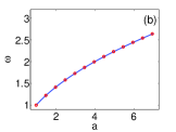
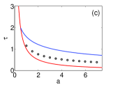
Figure 4: Comparison of numerical simulations (red circular markers) with the analytical expressions (continuous blue curve) given by Eq. (24) for (a) the radius and (b) the frequency of the ring state.(c) For each value of $a$, the time delay was chosen as $\tau=1/\sqrt{a-1/4}$ (black circular markers).

We have numerically computed the radius and angular frequency for different values of $a$ and $\tau$ within the region in which the mean field approximation gives a stable stationary center of mass (Fig. 4). Figures 4-4 shows that there is excellent agreement between the numerical simulations and the analytical result given by Eq. (24). It is worth noting that the condition given by Eq. (29) and used to derive Eq. (24) is satisfied in the long time limit in our simulations.

V-B The Rotating State

We show in Appendix B that the circular orbit of the rotating state has radius $\rho_{0}$ and frequency $\omega$ that satisfy the following relations:

$$\omega^{2}= a\cdot(1-\cos\omega\tau),$$ (25a)

$$\rho_{0}= \frac{1}{|\omega|}\sqrt{1-a\frac{\sin\omega\tau}{\omega}}.$$ (25b)

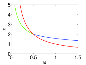
Figure 5: In $(a$,$\tau)$ space, we plot: Hopf (blue) and pitchfork (red) bifurcation curves, and the curve $a\tau^{2}=2$ where the first limit cycle ceases to exist by having its radius diverging to infinity (green).

Eqs. (25a)-(25b) can have as many solutions as desired by choosing $a$ and $\tau$ large enough. However, a careful analysis reveals that the solutions to Eqs. (25a)-(25b) are generated exactly along the Hopf curves of our previous mean field analysis and represent the same limit cycles of that analysis [Fig. 1]. The expressions in Eqs. (25a)-(25b) thus determine the spatio-temporal scales of these circular orbits beyond the Hopf curves where they are born. Our analysis also shows that the circular limit cycle that is created on the first member of the Hopf bifurcation curves persists to the left of the pitchfork bifurcation curve and then ceases to exist as its radius diverges to infinity on the curve $a\tau^{2}=2$ (Fig. 5). Moreover, numerical simulations of the mean field equations reveal that both the translating state and the rotating state are linearly stable for $(a,\tau)$ pairs inside the wedge between the curve $a\tau^{2}=2$ and the pitchfork bifurcation curve $a\tau=1$ above the BT point.

Figures 6-6 show the excellent agreement between numerical simulations and the analytical results given by Eqs. (25a)-(25b), for different values of $a$ and $\tau$.

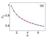
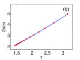
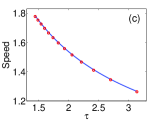
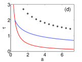
Figure 6: Comparison of numerical simulations (red circular markers) with the analytical expressions (continuous blue curve) given by Eqs. (25a)-(25b) for (a) the radius, (b) the period, and (c) the speed of the collapsed circular orbit. (d) For each value of $a$, the time delay was chosen as $\tau=\frac{2}{\sqrt{2a-1}}\arctan\left(\frac{\sqrt{2a-1}}{1-a}\right)$ (black circular markers) to assure asymptotic time convergence to the collapsed circular orbit state.

Interestingly, in Fig. 6 we note that in the asymptotic time limit the collapsed agents move at a speed greater than one, the speed at which agents would tend to move in the absence of coupling. This is explained by noting that the ratio of the time delay to the period of oscillations is such that the delayed position of the collapsed agents $\mathbf{R}(t-\tau)$ is ahead of the present position $\mathbf{R}(t)$. The attraction that an individual particle feels to the delayed position of the rest of the swarm forces the whole system go faster.

V-C The Degenerate Rotating State

A degenerate version of the rotating state is possible when the initial motion of the swarm is restricted to a line, since in this case it follows from Eqs. (1a)-(1b) that the swarm will remain on such a line for all times. As we show in Appendix C, we may assume that the motion of the collapsed swarm occurs on the $X=Y$ line of the center of mass coordinates and then use a finite Fourier mode approximation of the ensuing dynamics. An approximation in terms of just three modes gives

$$X(t)=Y(t)=2c_{1}\cos\omega t+2|c_{3}|\cos(3\omega t+\phi_{3}),$$ (26)

where $\omega$, $c_{1}$, $c_{3}$ and $\phi_{3}$ are obtained by solving Eqs. (42a)-(42b) numerically.

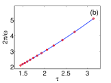
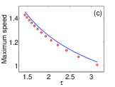
Figure 7: Comparison of numerical simulation (red circular markers) with the analytical expressions (continuous blue curve) given by Eqs. (42a)-(42b) for (a) the amplitude, (b) period, and (c) the maximum speed of the collapsed straight line orbit. (d) At each value of $a$, the time delay was chosen as $\tau=\frac{2}{\sqrt{2a-1}}\arctan\left(\frac{\sqrt{2a-1}}{1-a}\right)$ (black circular markers) to ensure asymptotic time convergence to the collapsed-straight line orbit state.

Figures 7-7 show a comparison between our analytical results given by Eqs. (42a)-(42b) and results obtained using numerical simulation for the amplitude, period and maximum speed of oscillation for different values of $a$ and $\tau$. There is excellent agreement in both amplitude and period between our analysis and the numerical simulations [Figs. 7-7]. The agreement for the speed of motion is very good as well, but the theoretical estimate is shifted slightly with respect to the results from simulations [Fig. 7]. As in the collapsed circular orbit, we note that the collapsed set of particles have a maximum speed which exceeds one, the speed that individual, uncoupled particles acquire in the long-time limit. As before, this effect arises from the attraction that the current particle position $\mathbf{R}(t)$ feels towards the delayed position $\mathbf{R}(t-\tau)$ when the latter lies in the direction of motion of the collapsed particles.

VI The Effects of Noise on the Swarm

In the absence of noise, the initial alignment of the swarm particles is critical in determining the asymptotic behavior of the swarm (Sec. V). When noise is introduced, the interplay of coupling strength, time delay and noise intensity gives rise to very interesting behavior due to fluctuations in the particles’ alignment. Specifically, our studies show that if the coupling strength $a$ and/or the time delay $\tau$ are below a certain limit, then the presence of noise promotes swarm transitions from aligned into misaligned coherent states. More surprising, however, is that if the coupling strength $a$ and/or the time delay $\tau$ are big enough, then there is a noise intensity threshold that forces a transition in the swarm from misaligned into aligned states. In addition, we show that for these high values of $a$ and/or $\tau$, the system presents an interesting hysteresis phenomenon when the noise intensity is time dependent.

For the purpose of these studies, we define the alignment of particle $j$ with the rest of the swarm as the cosine of the angle between the velocity of particle $j$ and the velocity of the swarm as a whole:

$$\cos\theta_{j}=\frac{\dot{\mathbf{r}}_{j}\cdot\dot{\mathbf{R}}}{|\dot{\mathbf{r}}_{j}||\dot{\mathbf{R}}|}.$$ (27)

Therefore the alignment of individual particles ranges from -1 to 1. A good measure of the overall alignment of the swarm is furnished by the ensemble average of these cosines given as

$$\textrm{Mean swarm alignment}=\frac{1}{N}\sum_{j=1}^{N}\cos\theta_{j}=\frac{1}{N}\sum_{j=1}^{N}\frac{\dot{\mathbf{r}}_{j}\cdot\dot{\mathbf{R}}}{|\dot{\mathbf{r}}_{j}||\dot{\mathbf{R}}|}.$$ (28)

We first carry out a numerical simulation with coupling constant $a=0.5$ and noise standard deviation $\sigma=0.05$ (noise intensity $D=0.00125$). At $t=50$, a time delay of $\tau=0.5$ is turned on. These parameters correspond to region A of Fig. 3. Initially, we place all particles at the origin and align their velocities by choosing $\dot{x}_{j}=1$ and $\dot{y}_{j}=1$ for all particles. We describe the behavior of the swarm by following the ensemble averages of the particle distances to the center of mass [Fig. 8] and of the particle alignment [Fig. 8] as functions of time. Before the time delay is turned on at $t=50$, the swarm is in a translating state with particles slightly spread out from the center of mass in a ‘pancake’ shape, as described in [23], with an ensemble alignment close to one. Once the delay is turned on, the translating state is broken up and the swarm converges to the ring state in which the mean particle alignment is near zero. The radius of the ring obtained in this numerical simulation matches the theoretical result [Eq. (24)] that predicts a radius of $\frac{1}{\sqrt{a}}=\sqrt{2}\approx 1.41$. A completely analogous situation ensues for parameters in region B of Fig. 3 (results not shown). In addition, in both cases the swarm will immediately converge to the ring state if the swarm velocities are not sufficiently aligned at time zero. We thus conclude that for these choices of $(a,\ \tau)$ pairs, the noise misaligns the particles’ velocities and forces a transition into the ring state.

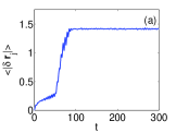
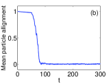
Figure 8: Time evolution of the ensemble average of (a) the particle distance to the center of mass, and (b) the mean particle alignment showing how the particle alignment breaks up due to the effects of noise. For long times the swarm converges to a ring state. The parameter values of $a=0.5$ and $\tau=0.5$ are associated with region A of Fig. 3. The time delay is turned on at $t=50$ and the noise standard deviation is $\sigma=0.05$ ($D=0.00125$).

In contrast to the cases discussed above, for parameters in region C of Fig. 3, a sufficiently large noise intensity promotes transitions from misaligned to aligned states. We show this by comparing the results of a series of simulations for different values of the noise standard deviation $\sigma$. The simulations are divided into two cases that differ only on the initial conditions for the swarm particles. In all simulations, the coupling constant $a=2$ and a time delay of $\tau=2$ is turned on at $t=50$. In the first case, all particles start from the origin with identical velocities $\dot{x}_{j}=1$ and $\dot{y}_{j}=1$. In the second case, all swarm particles are initially distributed uniformly on the unit square and are at rest.

In these simulations, the final state of the swarm may be visualized by plotting the mean swarm alignment after transients have decayed ($t=300$) as a function of noise intensity for the first case [Fig. 9] and the second case [Fig. 9]. In the first case of simulations, the high initial alignment of particles’ velocities forces the swarm to converge to a compact rotating state independent of noise intensity. However, the rotational state is destroyed if the noise standard deviation is bigger than $\sigma\approx 0.8$ [Fig. 9]. The situation is more interesting and complex for the second set of simulations. For low noise intensities ($\sigma\lesssim 0.26$) the low initial alignment of the particles leads the swarm to converge to a ring state with near zero mean alignment [Fig. 9]. A noise standard deviation just beyond the threshold of $\sigma\approx 0.26$ displays an interesting effect.

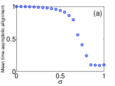
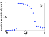
Figure 9: Asymptotic value of the mean particle alignment for (a) particles starting with perfectly aligned velocities at time zero and (b) for particles distributed uniformly over the unit square and starting from rest for different values of the noise standard deviation $\sigma$. The parameter values of $a=2$ and $\tau=2$ (turned on at $t=50$) are associated with a location in region C of Fig. 3.

As the $\sigma\approx 0.26$ threshold is crossed, the swarm transitions from the ring state into the rotating state with high mean alignment. An examination of the full simulation data reveals that the transition occurs as an increasing group of particles gradually becomes aligned and eventually absorbs all the remaining particles. A sufficient amount of noise is necessary for this transition, since it allows each particles’ velocity vector to probe many directions until finally enough of them become trapped in a ‘potential well’ of alignment with other particles. As with the first case of simulations a noise standard deviation bigger than $\sigma\approx 0.8$ breaks up the rotating state. Figure 10 clearly shows the transition from the ring to the compact, rotational state through the time evolution of the ensemble averages of the particle distances to the center of mass and of the mean particle alignment.

Further studies on the switching behavior between coherent states of the swarm demonstrate that the system exhibits a hysteresis phenomena. With the swarm system starting on the ring state with noise standard deviation of $\sigma=0.24$, one can force a transition into the rotating state by increasing the noise to $\sigma=0.26$. However, even if the noise is lowered down to $\sigma=0.02$, the swarm remains in the rotating state with a high velocity alignment [Figs. 11-11]. Nevertheless, it is possible to return the swarm to the ring state if, once in the rotating state, the noise is raised to very high amounts ($\sigma=1$) for a sufficient amount of time and then dropped suddenly to a very low value ($\sigma=0.05$). The high noise levels serve to completely misalign the particles’ velocities and allow them to converge to the ring once the noise levels are below $\sigma\lesssim 0.26$.

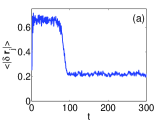
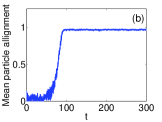
Figure 10: Time evolution of the ensemble average of (a) the particle distance to the center of mass, and (b) the mean particle alignment showing how the swarm transitions from a ring state into a compact, rotational state with alignment close to one. The parameter values of $a=2$ and $\tau=2$ (turned on at $t=50$) and $\sigma=0.4$ ($D=0.08$) are associated with region C of Fig. 3. Particles are initially distributed uniformly over the unit square and start from rest.

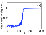
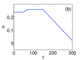
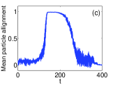
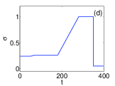
Figure 11: Time evolution of (a) mean particle alignment for example 1, (b) noise standard deviation for example 1, (c) mean particle alignment for example 2, and (d) noise standard deviation for example 2. The results show how a time-dependent noise intensity may be used to force swarm transitions. The parameter values of $a=2$ and $\tau=2$ (turned on at $t=10$) are associated with region C of Fig. 3. Particles are initially distributed uniformly over the unit square and start from rest.

VII Conclusions

In this work we analyzed the dynamics of a self-propelling swarm where individuals interact with a communication time delay in the presence of noise. Using a mean field approximation in the deterministic case, we analytically obtained the complete bifurcation picture in the parameter space of coupling strength and communication time delay. This analysis shows how different combinations of coupling strength and time delay induce the swarm to adopt different coherent structures asymptotically in time. Our bifurcation studies demonstrated the existence of a Bogdanov-Takens point, where the stationary center of mass solution has a double zero eigenvalue, which is critical in organizing the dynamics of the swarm.

The stable patterns that are possible for this system have several applications for autonomous vehicles. More detailed applications for each pattern are as follows: (1) the translational state may be used for target tracking and group transport [11, 17]. (2) The ring state should prove useful in terrain coverage and regional surveillance [39, 40]. (3) The rotating state may be exploited in obstacle avoidance, boundary tracking and surveillance [15, 11, 40]. In addition, we believe all three patterns are applicable to the problem of environmental sensing [13, 16].

In numerical experiments with noise, we showed that the interplay of coupling strength, time delay and noise intensity may give rise to interesting switching behavior from one coherent structure to another. We found that if the coupling strength $a$ and/or the time delay $\tau$ are below a certain limit, then the presence of noise induces transitions from states in which the alignment of the particles’ velocities is high into states with low alignment. More surprising, however, is that if the coupling strength $a$ and/or the time delay $\tau$ are big enough, then there is a noise intensity threshold that forces a transition in the swarm from misaligned into aligned states. In addition, by using a time-dependent noise intensity at these high values of $a$ and/or $\tau$, we show that the system exhibits hysteresis since the swarm’s transitions are not easily reversible. We note that analytical results on the effects of noise on delay-coupled swarms are not easy to obtain. Two examples relevant to our work are given in [23, 24], where the authors investigate models similar to the one presented here but without time delay.

Realistic application of the model treated here to the motion of multi-robot systems requires local repulsion among individuals to be taken into account. We have simulated the swarm model with the addition of a repulsive inter-agent potential of exponential form $U_{ij}=c_{r}\exp{\left({-\frac{|\mathbf{r}_{i}-\mathbf{r}_{j}|}{L_{r}}}\right)}$. These simulations demonstrate (results not shown) that the coherent patterns we discussed in this article persist when the characteristic repulsion length $L_{r}$ and repulsion strength $c_{r}$ between robots are small compared to global attraction parameters. Stronger repulsion can destabilize the coherent structures.

Recently, systems with non-uniform time delays have received much attention. For example, the important question of synchronization in networks communicating at randomly-distributed time delays has been recently investigated [41, 42]. In practical applications, the case of differing (and even time-varying) time delays between agents may be treated similarly to the case of a single delay by using a data buffer [27]. The idea is to identify an upper bound to the time delay ($\tau_{\textrm{max}}$) between all agent pairs and then design the agents so that the actuation occurs when the data buffer of size $\tau_{\textrm{max}}$ is full.

As part of our ongoing work, we are extending our investigations for the cases in which: (i) the communication time delays vary between different pairs of agents; and (ii) the communication graph is non-globally coupled. In realistic settings, both of these cases may occur due to the effects of the spatial distribution of agents such as signal travel times and imperfect transmission arising, for example, from complex terrain topography or component malfunction. In the case of communication delays that differ among different pairs of agents (though constant in time), our preliminary results show some patterns analogous to the ones observed here, but with much more added complexity. The present investigation lays a good foundation on which to base the study of these more complicated cases.

In summary, our results aid in understanding the stability of complex coherent structures in swarming systems with time delayed communication and in the presence of a noisy environment. Although our analytical and numerical results were obtained using a model with linear, attractive interactions, our analysis gives useful insight for the study of models with more general forms of time delayed coupling between agents. Our results may prove to be valuable for the control of man-made vehicles where actuation and communication are delayed, as well as in understanding swarm alignment in biological systems.

Appendix A Analysis of the Ring State

The swarm ring state is obtained when the center of mass is stationary. For the solution $\mathbf{R}=$const. to satisfy Eq. (III) we require

$$\sum_{i=1}^{N}\delta\dot{\mathbf{r}}_{i}^{2}\delta\dot{\mathbf{r}_{i}}=0.$$ (29)

We simplify Eq. (III) by taking $\mathbf{R}=$const. and using Eq. (29) we obtain

$$\delta\ddot{\mathbf{r}}_{j}= \left(1-\delta\dot{\mathbf{r}}_{j}^{2}\right)\delta\dot{\mathbf{r}}_{j}-a\delta\mathbf{r}_{j}-\frac{a}{N}\delta\mathbf{r}_{j}(t-\tau).$$ (30)

We consider the large system size limit $N\rightarrow\infty$ and we drop the delayed term. The resulting equations are simply ODEs and so the analysis below shows that the ring orbit is not dependent on having time delays in the system. Writing Eq. (30) in polar coordinates $\delta x_{j}=\rho_{j}\cos{\theta_{j}}$ and $\delta y_{j}=\rho_{j}\cos{\theta_{j}}$, we obtain

$$\ddot{\rho}_{j}= \left(1-\dot{\rho}_{j}^{2}-\rho_{j}^{2}\dot{\theta}_{j}^{2}\right)\dot{\rho}_{j}+\rho_{j}\dot{\theta}_{j}^{2}-a\rho_{j},$$ (31a)

$$\rho_{j}\ddot{\theta}_{j}= \left(1-\dot{\rho}_{j}^{2}-\rho_{j}^{2}\dot{\theta}_{j}^{2}\right)\rho_{j}\dot{\theta}_{j}-2\dot{\rho}_{j}\dot{\theta}_{j}.$$ (31b)

Equations (31a)-(31b) have the trivial solution $\rho_{j}=0$ as well as a ring solution:

$$\rho_{j}=\frac{1}{\sqrt{a}},\qquad\dot{\theta}_{j}=\pm\sqrt{a},$$ (32)

in which particles move at unit speed, $\rho_{j}\dot{\theta}_{j}=\pm 1$.

Appendix B Analysis of the Rotating State

In the noiseless rotating state, all particles collapse to a point, $\delta\mathbf{r}_{i}=0$, and the equation for the center of mass given by Eq. (III) simplifies considerably to

$$\ddot{\mathbf{R}}= \left(1-\dot{\mathbf{R}}^{2}\right)\dot{\mathbf{R}}-a\left(\mathbf{R}(t)-\mathbf{R}(t-\tau)\right).$$ (33)

We write $\mathbf{R}=(X,Y)$ and introduce polar coordinates $X=\rho\cos{\theta}$ and $Y=\rho\sin{\theta}$ to obtain

$$\ddot{\rho}= \left(1-\dot{\rho}^{2}-\rho^{2}\dot{\theta}^{2}\right)\dot{\rho}+\rho\dot{\theta}^{2}-a\bigg{(}\rho-\rho_{\tau}\cos(\theta-\theta_{\tau})\bigg{)},$$ (34a)

$$\rho\ddot{\theta}= \left(1-\dot{\rho}^{2}-\rho^{2}\dot{\theta}^{2}\right)\rho\dot{\theta}-2\dot{\rho}\dot{\theta}+a\rho_{\tau}\sin(\theta-\theta_{\tau}),$$ (34b)

where we’ve written $\rho_{\tau}\equiv\rho(t-\tau)$ and $\theta_{\tau}\equiv\theta(t-\tau)$. Equations (34a)-(34b) have a circular orbit solution, $\rho=\rho_{0}$ and $\theta=\omega t+\theta_{0}$, where

$$\omega^{2}= a\cdot(1-\cos\omega\tau),$$ (35a)

$$\rho_{0}= \frac{1}{|\omega|}\sqrt{1-a\frac{\sin\omega\tau}{\omega}}.$$ (35b)

and $\theta_{0}$ is obtained from the initial conditions. In the main text we discuss the behavior of the solutions to Eqs. (35a)-(35b).

Appendix C Analysis of the Degenerate Rotating State

When the motion of the whole swarm is initially constrained to a line, Eqs. (1a)-(1b) dictate that the swarm will remain on this line for all times. If the coupling parameter $a$ and/or the time delay $\tau$ are large enough, the resulting motion is a degenerate form of the rotating solution in which the swarm moves back and forth along a straight line.

In the case without noise all particles collapse to a point, $\delta\mathbf{r}_{i}=0$, and the line along which motion occurs is arbitrary; here we use $X=Y$. The problem reduces to analyzing a single delay equation given by

$$\ddot{X}= \left(1-2\dot{X}^{2}\right)\dot{X}-a\left(X(t)-X(t-\tau)\right).$$ (36)

We find a solution using Fourier analysis. We let

$$X(t)=\sum_{n=-\infty}^{\infty}c_{n}e^{in\omega t},$$ (37)

where the coefficients satisfy $c_{n}={c_{-n}}^{*}$ in order to ensure that $X(t)$ is a real quantity. Substituting Eq. (37) into Eq. (36), we get for the $n$-th mode

$$-n^{2}\omega^{2}c_{n} =in\omega c_{n}$$

$$+2i\omega^{3}\sum_{\ell,m\neq 0}c_{\ell}c_{m}c_{n-\ell-m}\ell m(n-\ell-m)$$

$$-ac_{n}(1-e^{-in\omega\tau}),$$ (38)

for $n=0,1,2,\dots$. The $n=0$ equation is

$$\sum_{\ell,m\neq 0}c_{\ell}c_{m}c_{-\ell-m}\ell m(\ell+m)=0,$$ (39)

which does not involve $c_{0}$. Unsurprisingly, $c_{0}$ is undetermined since the position of the center of mass may be translated in space without modifying the dynamics of the system.

We now approximate the motion of the center of mass by keeping the first three modes. By appropriately choosing the time origin, we may take $c_{1}$ to be purely real and positive. In contrast, $c_{2}$ and $c_{3}$ are complex quantities which we write as $c_{i}=|c_{i}|e^{i\phi_{i}}$, for $i=2,3$. The equations for the first three modes $n=1,2,3$ become

$$- \omega^{2}c_{1}=i\omega c_{1}$$

$$+2i\omega^{3}\left(-3c_{1}^{3}-36c_{2}^{2}c_{3}^{*}-54c_{1}|c_{3}|^{2}-24c_{1}|c_{2}|^{2}+9c_{1}^{2}c_{3}\right)$$

$$-ac_{1}(1-e^{-i\omega\tau}),$$ (40a)

$$- 4\omega^{2}c_{2}=2i\omega c_{2}$$

$$+2i\omega^{3}\left(-108c_{2}|c_{3}|^{2}-36c_{1}c_{2}^{*}c_{3}-24c_{2}|c_{2}|^{2}-12c_{2}c_{1}^{2}\right)$$

$$-ac_{2}(1-e^{-2i\omega\tau}),$$ (40b)

$$- 9\omega^{2}c_{3}=3i\omega c_{3}$$

$$+2i\omega^{3}\left(-18c_{3}c_{1}-72c_{3}|c_{2}|^{2}-81c_{3}|c_{3}|^{2}-12c_{2}^{2}c_{1}+c_{1}^{3}\right)$$

$$-ac_{3}(1-e^{-3i\omega\tau}).$$ (40c)

In addition, the condition from Eq.(39) becomes

$$6(c_{2}c_{3}^{*}-c_{2}^{*}c_{3})-c_{1}(c_{2}-c_{2}^{*})=0.$$ (41)

Separating Eqs. (40a)-(40c) and Eq. (41) into real and imaginary parts yields a system of seven equations (since the real part of Eq. (41) is satisfied automatically) for the six unknowns: $\omega$, $c_{1}$, $|c_{2}|$, $\phi_{2}$, $|c_{3}|$ and $\phi_{3}$. These equations cannot be satisfied in general. However, if $|c_{2}|=0$, then the equation for mode $n=2$ [Eq. (40b)] and Eq. (41) are satisfied automatically, leaving four equations:

$$-\omega^{2}c_{1}= i\omega c_{1}+2i\omega^{3}\left(-3c_{1}^{3}54c_{1}|c_{3}|^{2}+9c_{1}^{2}c_{3}\right)$$

$$-ac_{1}(1-e^{-i\omega\tau}),$$ (42a)

$$-9\omega^{2}c_{3}= 3i\omega c_{3}+2i\omega^{3}\left(-18c_{3}c_{1}-81c_{3}|c_{3}|^{2}+c_{1}^{3}\right)$$

$$-ac_{3}(1-e^{-3i\omega\tau}).$$ (42b)

for the four unknowns $\omega$, $c_{1}$, $|c_{3}|$ and $\phi_{3}$. Equations (42a)-(42b) may be solved numerically and permit one to approximate the motion of the center of mass in the form

$$X(t)=Y(t)=2c_{1}\cos\omega t+2|c_{3}|\cos(3\omega t+\phi_{3}).$$ (43)

The frequency of the straight line orbit of the swarm center of mass is approximately equal to the frequency of the circular orbit in Eq. (25a). In addition, the amplitude of oscillation of the straight line orbit is approximately equal to the radius of the circular orbit of Eq. (25b) divided by a factor of $\sqrt{6}$.

References

- [1] E. Budrene and H. Berg, “Dynamics of formation of symmetrical patterns by chemotactic bacteria,” Nature, vol. 376, no. 6535, pp. 49–53, 1995.
- [2] J. Toner and Y. Tu, “Long-range order in a two-dimensional dynamical xy model: How birds fly together,” Phys. Rev. Lett., vol. 75, no. 23, pp. 4326–4329, 1995.
- [3] ——, “Flocks, herds, and schools: A quantitative theory of flocking,” Phys. Rev. E, vol. 58, no. 4, pp. 4828–4858, 1998.
- [4] J. K. Parrish, “Complexity, pattern, and evolutionary trade-offs in animal aggregation,” Science, vol. 284, no. 5411, pp. 99–101, Apr 1999.
- [5] L. Edelstein-Keshet, J. Watmough, and D. Grunbaum, “Do travelling band solutions describe cohesive swarms? an investigation for migratory locusts,” J. Math. Biol., vol. 36, no. 6, pp. 515–549, 1998.
- [6] C. Topaz and A. Bertozzi, “Swarming patterns in a two-dimensional kinematic model for biological groups,” SIAM J. Appl. Math., vol. 65, no. 1, pp. 152–174, 2004.
- [7] D. Hebling and P. Molnar, “Social force model for pdestrian dynamics,” Phys. Rev. E., vol. 51, pp. 4282–4286, 1995.
- [8] A.H. Cohen, P.J. Holmes and R.H. Rand. “The Nature of the Coupling Between Segmental Oscillators of the Lamprey Spinal Generator for Locomotion: A Mathematical Model,” J. Math. Biol., vol. 13, pp. 345, 1982.
- [9] N. Leonard and E. Fiorelli, “Virtual leaders, artificial potentials and coordinated control of groups,” Proc. IEEE Conf. Decis. Control, vol. 3, pp. 2968–2973, 2002.
- [10] E. Justh and P. Krishnaprasad, “Steering laws and continuum models for planar formations,” Proc. IEEE Conf. Decis. Control, vol. 4, pp. 3609–3614, 2004.
- [11] D. Morgan and I. Schwartz, “Dynamic coordinated control laws in multiple agent models,” Phys. Lett. A, vol. 340, no. 1-4, pp. 121–131, 2005.
- [12] Y.-L. Chuang, Y. R. Huang, M. R. D’Orsogna, and A. L. Bertozzi, “Multi-vehicle flocking: Scalability of cooperative control algorithms using pairwise potentials,” Proc. IEEE Int. Conf. Robot. Automat., pp. 2292–2299, 2007.
- [13] K. M. Lynch, P. Schwartz, I. B. Yang, and R. A. Freeman, “Decentralized environmental modeling by mobile sensor networks,” IEEE Trans. Robotics, vol. 24, no. 3, pp. 710–724, 2008.
- [14] B. Nguyen, Y.-L. Chuang, D. Tung, C. Hsieh, Z. Jin, L. Shi, D. Marthaler, A. Bertozzi, and R. Murray, “Virtual attractive-repulsive potentials for cooperative control of second order dynamic vehicles on the Caltech MVWT,” Proc. Amer. Control Conf., vol. 2, pp. 1084 – 1089, June 2005.
- [15] C. Hsieh, Z. Jin, D. Marthaler, B. Nguyen, D. Tung, A. Bertozzi, and R. Murray, “Experimental validation of an algorithm for cooperative boundary tracking,” Proc. Amer. Control Conf., pp. 1078–1083, 2005.
- [16] B. Lu, J. Oyekan, D. Gu, H. Hu, and H. F. G. Nia, “Mobile sensor networks for modelling environmental pollutant distribution,” Int. J. Syst. Sci, vol. 42, no. 9, SI, pp. 1491–1505, 2011.
- [17] T. Chung, J. Burdick, and R. Murray, “A decentralized motion coordination strategy for dynamic target tracking,” in Proc. IEEE Int. Conf. Robot. Automat., pp. 2416–22, 2006.
- [18] A. Papachristodoulou and A. Jadbabaie, “Synchronization in oscillator networks with heterogeneous delays, switching topologies and nonlinear dynamics,” IEEE Conf. Decis. Control, pp. 4307 – 4312, 2007.
- [19] T. W. Mather and M. A. Hsieh, “Macroscopic modeling of stochastic deployment policies with time delays for robot ensembles,” Int. J. Rob. Res., vol. 30, no. 5, pp. 590–600, APR 2011.
- [20] T. Vicsek, A. Czirók, E. Ben-Jacob, I. Cohen, and O. Shochet, “Novel type of phase transition in a system of self-driven particles,” Phys. Rev. Lett., vol. 75, no. 6, pp. 1226–1229, 1995.
- [21] G. Flierl, D. Grünbaum, S. Levins, and D. Olson, “From individuals to aggregations: the interplay between behavior and physics,” J. Theor. Biol., vol. 196, no. 4, pp. 397–454, 1999.
- [22] I. Couzin, J. Krause, R. James, G. Ruxton, and N. Franks, “Collective memory and spatial sorting in animal groups,” J. Theor. Biol., vol. 218, no. 1, pp. 1–11, 2002.
- [23] U. Erdmann and W. Ebeling, “Noise-induced transition from translational to rotational motion of swarms,” Phys. Rev. E, vol. 71, 051904, 2005.
- [24] J. Strefler, U. Erdmann and L. Schimansky-Geier, “Swarming in three dimensions,” Phys. Rev. E, vol. 78, 031927, 2008.
- [25] E. Forgoston and I. Schwartz, “Delay-induced instabilities in self-propelling swarms,” Phys. Rev. E, vol. 77, 035203(R), 2008.
- [26] M. Kimura and J. Moehlis, “Novel vehicular trajectories for collective motion from coupled oscillator steering control,” SIAM J. Appl. Dyn. Syst., vol. 7, pp. 1191–1212, 2008.
- [27] B. Yang and H. Fang, “Forced consensus in networks of double integrator systems with delayed input,” Automatica, vol. 46, pp. 629–632, 2010.
- [28] M. Aldana, V. Dossetti, C. Huepe, V. Kenkre, and H. Larralde, “Phase transitions in systems of self-propelled agents and related network models,” Phys. Rev. Lett., vol. 98, 095702, 2007.
- [29] N. MacDonald, Time Lags in Biological Models, 1st ed. Berlin: Springer-Verlag, 1978.
- [30] ——, Biological Delay Systems Models: Linear Stability Theory, 1st ed. Cambridge: Cambridge University Press, 1989.
- [31] I. Ncube, S. A. Campbell, and J. Wu, “Change in criticality of synchronous Hopf bifurcation in a multiple-delayed neural system,” Fields Inst. Commun., vol. 36, pp. 179–193, 2003.
- [32] S. Bernard, J. Bélair, and M. Mackey, “Bifurcations in a white-blood-cell production model,” C.R. Biol., vol. 327, pp. 201–210, 2004.
- [33] M. Mackey, M. Santillan, and N. Yildirim, “Modeling operon dynamics: The Tryptophan and lactose operons as paradigms,” C.R. Biol., vol. 327, pp. 211–224, 2004.
- [34] M. Mackey and M. Santillan, “Why is the lysogenic state of phage- is so stable: A mathematical modelling approach,” Biophys. J., vol. 86, pp. 75–84, 2004.
- [35] G. Tiana, M.H. Jensen, and K. Sneppen, “Time delay as a key to apoptosis in the p53 network,” Eur. Phys. J. B, vol. 29, pp. 135–140, 2002.
- [36] M.H. Jensen, K. Sneppen, and G. Tiana, “Sustained oscillations and time delays in gene expression of protein Hes1,” FEBS Lett., vol. 541, pp. 176–177, 2003.
- [37] N. Monk, “Oscillatory expression of Hes1, p53, and NF-B driven by transcriptional time delays,” Curr. Biol., vol. 13, pp. 1409–1413, 2003.
- [38] K. Engelborghs, “DDE-BIFTOOL: A matlab package for bifurcation analysis of delay differential equations,” Department of Computer Science, K. U. Leuven, Belgium, Tech. Rep. TW-305, 2000. [Online]. Available: http://www.cs.kuleuven.ac.be/twr/research/software/delay/ddebiftool.shtml
- [39] J. Svennebring and S. Koenig, “Trail-Laying Robots for Robust Terrain Coverage,” Proc. IEEE Int. Conf. Robot. Automat., pp. 75, 2003.
- [40] D. Vallejo, P. Remagnino, D.N. Monekosso, L.J. and C. Gonzalez. “A Multi-agent Architecture for Multi-robot Surveillance, ”Lecture Notes in Computer Science, vol. 5796, pp. 266, Springer, 2003.
- [41] C. Masoller, and A. C. Marti, “Random Delays and the Synchronization of Chaotic Maps,” Phys. Rev. Lett., vol. 94, pp. 134102, 2005.
- [42] A.C. Marti, M. Ponce and C. Masoller, “Chaotic maps coupled with random delays: connectivity, topology, and network propensity for synchronization ,” Physica A, vol. 371, pp. 104–107, 2006.