Distributed Linear Precoder Optimization and Base Station Selection for an Uplink Heterogeneous Network

Abstract

In a heterogeneous wireless cellular network, each user may be covered by multiple access points such as macro/pico/relay/femto base stations (BS). An effective approach to maximize the sum utility (e.g., system throughput) in such a network is to jointly optimize users’ linear procoders as well as their base station associations. In this paper we first show that this joint optimization problem is NP-hard and thus is difficult to solve to global optimality. To find a locally optimal solution, we formulate the problem as a noncooperative game in which the users and the BSs both act as players. We introduce a set of new utility functions for the players and show that every Nash equilibrium (NE) of the resulting game is a stationary solution of the original sum utility maximization problem. Moreover, we develop a best-response type algorithm that allows the players to distributedly reach a NE of the game. Simulation results show that the proposed distributed algorithm can effectively relieve local BS congestion and simultaneously achieve high throughput and load balancing in a heterogeneous network.

I Introduction

Consider a multicell heterogeneous network (HetNet) in which every cell is installed with not only a macro base station (BS) but also a set of micro/pico/femto base stations, all equipped with multiple antennas and sharing the same frequency band. In such a network, the users are often simultaneously covered by multiple BSs with different capabilities and load status. If the users in a HetNet are assigned to BSs simply according to their received signal strengths (as is done in conventional cellular networks), then a BS located close to a hot spot may experience severe congestion, causing poor quality of service in the network. Indeed, it has been shown that the signal strength based approach for user-BS association in a HetNet can be highly suboptimal for congestion management and fairness provisioning [2, 3]. For a HetNet, the overall system performance depends not only on the physical layer choices of precoder design and power control, but also on how the users and the BSs are associated. Consequently, BS assignment should be an integral part of physical layer optimization of the overall system performance.

Conventionally, physical layer resource management and network performance optimization involve such aspects as transceiver design, power control and spectrum management, while the user-BS assignment is assumed known and fixed. For example, under this assumption, game theoretic approaches have been used to design optimal transmit precoders for a MIMO interference channel (MIMO-IC). The authors of [4, 5], among others, propose to formulate the transmit covariance matrix optimization problem as a noncooperative game in which the transmitters/users compete with each other for transmission. Reference [6] further takes into consideration the robustness issue of the problem. In these studies, each user selfishly maximizes its own transmission rate, while treating all other users’ interference as noise. Simple distributed algorithms (based on iterative water-filling) are derived with convergence guarantees, but the resulting solutions of the game are inefficient in terms of system throughput. This is due to both the lack of coordination among the transmitters/users and the choice of utility functions which do not consider the interference effect on other users in the system.

In addition to the competitive design, we can also design transmit precoders by maximizing a suitable system utility function. Unfortunately, most optimization problems in this category have been proven to be NP-hard in various settings [7, 8, 9, 10]. As a result, many authors focus on developing efficient algorithms to compute high quality sub-optimal solutions for these problems, e.g., in MIMO-IC, [11, 12], MISO-IC [13, 14, 15] and MIMO-IC with a single data stream per user [16, 17]. In particular, references [11, 12] propose an iterative algorithm based on the first order Taylor approximation of the nonconcave part of the weighted sum rate (WSR) objective. It is shown that the WSR values generated by this algorithm increase monotonically, but the convergence of the users’ transmit covariances (to a stationary solution) is left unproven. For the problem of maximizing a general utility function, reference [8] proposes a cyclic ascent method for linear precoder design in a MISO network. The proposed algorithm can deal with any smooth utility functions and is known to converge to a stationary solution. Reference [9] develops an algorithm that optimizes the Max-Min utility in a MIMO network by adapting the transmit and receive precoders alternately. References [18, 19] propose a weighted Minimum Mean Square Error (WMMSE) algorithm in which the transmitters and receivers iteratively update their linear transmit and receive strategies to optimize the system utility function. The authors show that as long as the system utility function satisfies some mild regularity conditions, their algorithm is guaranteed to converge to a stationary point of the problem.

All of the above cited works aim at optimizing the linear transceiver structures under the assumption that the transmitter-receiver association is known and fixed. The problem of joint cell site selection and power allocation in the traditional CDMA based network has been first considered in [20, 21, 22] and later in a game theoretical perspective in [23, 24]. The objective of the network optimization is to minimize the users’ total transmit power subject to a set of individual SNR constraints. In these works, the users optimize their uplink power levels and/or transmit beams as well as their BS associations. The phenomenon of “cell breathing” is observed whereby the sizes of the cells dynamically change according to the congestion levels. Recently references [25, 26, 27] have considered the joint BS selection and vector power allocation in OFDMA networks in which the BSs operate on non-overlapping spectrum. The users compete with each other for resources in each cell, and at the same time they are able to freely choose to use any (non-interfering) BS in the network. However, it is not clear how these works can be generalized to the considered MIMO-HetNet scenario. Reference [28] is a recent work in such direction. Differently from the present work, a downlink HetNet setting is considered. As a result, the user-BS association is determined in a centralized fashion, which is very different than the distributed solutions to be presented in this work.

In this paper, we consider the problem of joint optimization of linear precoder and BS assignment for an uplink MIMO heterogeneous network. Our main contributions are summarized as follows.

1. We establish the NP-hardness of the joint precoder design and user-BS assignment problem for the weighted sum rate (WSR) maximization in a MIMO-HetNet. This NP-hardness result is intrinsically different from the existing complexity results [7, 8, 9, 10] for the linear precoder design problem where the user-BS assignment is fixed. In particular, for the latter results, the NP-hardness of the precoder design problem lies in how to determine which users/antennas should be turned off due to strong interference links. However, when the user-BS assignment is not fixed, a strong interference link can be turned into a direct link by changing the user-BS association, thus effectively mitigating the level of interference. As a result, what makes the joint user-BS association and precoder design problem difficult is not the presence of strong interference links, but rather its mixed interference pattern. Therefore, the NP-hardness of the joint optimization problem does not follow from, nor imply, any of the existing complexity results [7, 8, 9, 10] for the linear precoder design problem when the user-BS assignment is fixed.

2. We propose a novel game theoretic formulation to find a local WSR-optimal solution of the joint precoder design and user-BS assignment problem for a MIMO heterogeneous network. In the proposed game both the transmitters and the BSs act as players. We introduce a set of utility functions for the players and show that every NE of the resulting game, which gives a set of precoders and user-BS assignment for all users in the network, is a stationary solution of the WSR maximization problem. To reach a NE of the game, each transmitter greedily determines the best linear precoder as well as the least congested BS for transmission, whereas each BS computes a set of optimal prices to charge the users for causing interference. These prices serve to coordinate the behavior of the users so that they do not cause excessive interference in the network. We show that the resulting distributed algorithm converges to a NE of the game. Notice that the convergence of the algorithm implies that the network will be stable in the sense that no user will change BSs indefinitely. Simulation results show that this algorithm is very effective in relieving local BS congestion and achieving high throughput and load balancing in the network.

We remark that when the user-BS assignment is fixed, our proposed game reduces to the standard precoder optimization game. In this context, the users are again charged with a set of prices that reflect their (negative) influence to other users. Thus, our problem formulation can be viewed as a generalization of previous results for interference pricing (e.g. [11, 15, 16, 29]) to the MIMO interfering multiple access channel (MIMO-IMAC) setting with general system utility functions.

The rest of the paper is organized as follows. In Section II, we give the system level description of the problem, and provide its complexity analysis. In Section III and Section IV, we formulate the problem into a non-cooperative game framework, and study the properties of the resulting games. Furthermore we propose an efficient algorithm to compute the equilibrium solutions of the games. In Section V, we present numerical results to demonstrate the performance of the proposed algorithm. Some concluding remarks are given in Section VI.

Notations: For a symmetric matrix $\mathbf{X}$, $\mathbf{X}\succeq 0$ signifies that $\mathbf{X}$ is positive semi-definite. We use ${\mbox{{Tr}}}(\mathbf{X})$, $|\mathbf{X}|$, $\mathbf{X}^{H}$, $\lambda(\mathbf{X})$ and ${\mbox{{Rank}}}(\mathbf{X})$ to denote the trace, determinant, Hermitian, spectral radius and the rank of a matrix, respectively. We use $\mathbf{I}_{n}$ to denote a $n\times n$ identity matrix, and use $[y,\mathbf{x}_{-i}]$ to denote a vector $\mathbf{x}$ with its $i^{th}$ elements replaced by $y$. Moreover, we let $\mathbb{R}^{N\times M}$ and $\mathbb{C}^{N\times M}$ denote the set of real and complex $N\times M$ matrices, and use $\mathbb{S}^{N}$ and $\mathbb{S}^{N}_{+}$ to denote the set of $N\times N$ Hermitian and Hermitian semi-definite matrices, respectively. Finally, we use the notation $0\leq a\perp b\geq 0$ to indicate $a\geq 0,b\geq 0,a\times b=0$, and use the notation $[x]^{+}$ to represent $\max(x,0)$.

II System Model, Problem Formulation and Complexity Result

We consider the uplink of a general MIMO-HetNet consisting of a set $\mathcal{N}=\{1,\cdots,N\}$ of users that transmit to a set $\mathcal{Q}=\{1,\cdots,Q\}$ of BSs. Let $\mathbf{a}$ be a $N\times 1$ vector representing the system association profile, i.e., $\mathbf{a}_{n}=q$ means user $n$ connects to BS $q$.

Suppose each user $n\in\mathcal{N}$ has $T_{n}$ transmit antennas and each BS $q\in\mathcal{Q}$ has $R_{q}$ receive antennas. Let $\mathbf{H}_{q,n}\in\mathbb{C}^{R_{q}\times T_{n}}$ be the channel matrix from transmitter $n$ to receiver $q$. Assume $T_{n}\leq R_{q}$ for all $(n,q)\in(\mathcal{N}\times\mathcal{Q})$, or equivalently the channel matrices $\{\mathbf{H}_{q,n}\}$ are tall matrices. This assumption is reasonable as the number of antennas at the BS is typically larger than that of the mobile users.

Let $\mathbf{x}_{n}\in\mathbb{C}^{T_{n}}$ and $\mathbf{y}_{q}\in\mathbb{C}^{R_{q}}$ denote the transmitted signal of user $n$ and the received signal of BS $q$, respectively. Then $\mathbf{y}_{q}$ can be expressed as

$$\mathbf{y}_{q}=\sum_{n\in\mathcal{N}}\mathbf{H}_{q,n}\mathbf{x}_{n}+\mathbf{z}_{q}$$ (1)

where $\mathbf{z}_{q}\sim\mathcal{CN}(0,\sigma^{2}_{q}\mathbf{I}_{R_{q}})$ is the additive white complex Gaussian noise vector. Suppose there are a maximum of $T_{n}$ data streams transmitted by user $n$ and its data symbol vector is denoted by $\mathbf{s}_{n}\in\mathbb{C}^{T_{n}}$. We assume $\mathbb{E}[\mathbf{s}_{n}\mathbf{s}_{n}^{H}]=\mathbf{I}_{T_{n}}$. If a linear precoder $\mathbf{P}_{n}\in\mathbb{C}^{T_{n}\times T_{n}}$ is used for transmission, then the transmitted vector of user $n$ is $\mathbf{x}_{n}=\mathbf{P}_{n}\mathbf{s}_{n},$ and the corresponding transmit covariance matrix $\mathbf{S}_{n}$ is given by $\mathbf{S}_{n}\triangleq\mathbb{E}[\mathbf{x}_{n}\mathbf{x}^{H}_{n}]=\mathbf{P}_{n}\mathbf{P}_{n}^{H}\in\mathbb{S}^{T_{n}}_{+}$. Once the covariance matrix $\mathbf{S}_{n}$ is computed, the precoder can be obtained by Cholesky factorization. We further assume that each user has an individual average power constraint of the form $\mathbb{E}[\mbox{Tr}(\mathbf{x}_{n}\mathbf{x}^{H}_{n})]=\mbox{Tr}(\mathbf{S}_{n})\leq\bar{p}_{n}$. Define the aggregate transmit covariance as $\mathbf{S}\triangleq\{\mathbf{S}_{n}\}_{n\in\mathcal{N}}$, and the aggregate covariance excluding user $n$ as $\mathbf{S}_{-n}\triangleq\{\mathbf{S}_{m}\}_{m\neq n,m\in\mathcal{N}}$.

For a fixed association profile $\mathbf{a}$, the interference covariance matrix for user $n$ (at its intended BS $\mathbf{a}_{n}$) can be expressed as

$$\mathbf{C}_{n}(\mathbf{S}_{-n};\mathbf{a})\triangleq\sigma^{2}_{\mathbf{a}_{n}}\mathbf{I}_{R_{\mathbf{a}_{n}}}+\sum_{m\neq n}\mathbf{H}_{\mathbf{a}_{n},m}\mathbf{S}_{m}\mathbf{H}^{H}_{\mathbf{a}_{n},m}.$$

The covariance matrix of the total received signal at BS $q$ can be expressed as

$$\mathbf{G}_{q}(\mathbf{S})\triangleq\sigma^{2}_{q}\mathbf{I}+\sum_{l=1}^{N}\mathbf{H}_{q,l}\mathbf{S}_{l}\mathbf{H}^{H}_{q,l}.$$ (2)

For a given user-BS association $\mathbf{a}$, the achievable rate for user $n$ is given by [30]

$$R_{n}(\mathbf{S}_{n},\mathbf{S}_{-n};\mathbf{a}) =\log\left|\mathbf{I}_{R_{\mathbf{a}_{n}}}+\mathbf{H}_{\mathbf{a}_{n},n}\mathbf{S}_{n}\mathbf{H}^{H}_{\mathbf{a}_{n},n}\mathbf{C}_{n}^{-1}(\mathbf{S}_{-n})\right|$$ (3)

$$=\log\left|\mathbf{I}_{T_{n}}+({{\mathbf{S}}}^{\frac{1}{2}}_{n})^{H}\mathbf{H}^{H}_{\mathbf{a}_{n},n}{\mathbf{C}}_{n}^{-1}({\mathbf{S}}_{-n})\mathbf{H}_{\mathbf{a}_{n},n}\mathbf{S}^{\frac{1}{2}}_{n}\right|$$

$$\stackrel{{\scriptstyle\mbox{\footnotesize(i)}}}{{=}}\log\left|\left(\mathbf{I}_{T_{n}}-(\mathbf{S}_{n}^{\frac{1}{2}})^{H}\mathbf{H}^{H}_{\mathbf{a}_{n},n}\mathbf{G}_{\mathbf{a}_{n}}^{-1}(\mathbf{S})\mathbf{H}_{\mathbf{a}_{n},n}\mathbf{S}^{\frac{1}{2}}_{n}\right)^{-1}\right|\stackrel{{\scriptstyle\mbox{\footnotesize(ii)}}}{{=}}\log\left|\mathbf{E}^{-1}_{n}(\mathbf{S})\right|$$ (4)

where in (i) we have used the matrix inversion lemma [31]; in (ii) we have defined $\mathbf{E}_{n}(\mathbf{S})$ as user $n$’s minimum mean square error (MMSE) matrix

$$\mathbf{E}_{n}(\mathbf{S}) \triangleq\mathbf{I}_{T_{n}}-(\mathbf{S}_{n}^{\frac{1}{2}})^{H}\mathbf{H}^{H}_{\mathbf{a}_{n},n}\mathbf{G}_{\mathbf{a}_{n}}^{-1}(\mathbf{S})\mathbf{H}_{\mathbf{a}_{n},n}\mathbf{S}^{\frac{1}{2}}_{n}\succ 0.$$ (5)

The WSR of the system can be expressed as $R(\mathbf{S};\mathbf{a})\triangleq\sum_{n\in\mathcal{N}}w_{n}R_{n}(\mathbf{S}_{n},\mathbf{S}_{-n};\mathbf{a})$, where the set of nonnegative weights $\{w_{n}\}_{n=1}^{N}$ represent the priorities of different users. We are interested in finding the optimal user-BS assignment as well as the transmit covariance matrices that maximize the WSR. This problem can be stated as

$$~{}~{}\max_{\mathbf{S},\mathbf{a}}R(\mathbf{S};\mathbf{a})$$ (SYS)

$$s.t. ~{}~{}\mbox{Tr}(\mathbf{S}_{n})\leq\bar{p}_{n},~{}\mathbf{S}_{n}\in\mathbb{S}^{T_{n}}_{+},~{}\forall~{}n\in\mathcal{N}$$

$$~{}~{}\mathbf{a}_{n}\in\mathcal{Q},~{}\forall~{}n\in\mathcal{N}.$$

Our first result shows that finding the global optimal solution to the system level problem is intractable in general.

Theorem 1

Finding the optimal BS association and the transmission covariance matrices $(\mathbf{a},\mathbf{S})$ that solve the problem (SYS) is strongly NP-hard.

Theorem 1 is proved based on a polynomial time transformation from the 3-SAT problem, which is a known NP-complete problem [32]. The 3-SAT problem is described as follows. Given $M$ disjunctive clauses $C_{1},\cdots,C_{M}$ defined on $N$ Boolean variables $X_{1}\cdots,X_{N}$, i.e., $C_{m}=t_{1}\vee t_{2}\vee t_{3}$ with $t_{i}\in\{X_{1},\cdots,X_{N},\bar{X}_{1},\cdots,\bar{X}_{N}\}$, the problem is to check whether there exists a truth assignment for the Boolean variables such that all clauses are satisfied (i.e., each clause evaluates to $1$) simultaneously. We leave the details of the proof to the Appendix A. We note that our complexity result differs from the recent result in [28], in which the complexity for the joint user-BS association and precoder design problem is analyzed for the downlink direction.

Motivated by the above complexity result, we focus on designing low complexity algorithms that can provide approximately optimal solutions. In particular, we will consider in the sequel a more general system level problem formulated as the following sum utility maximization problem

$$\max_{\mathbf{S},\mathbf{a}} \quad f(\mathbf{S};\mathbf{a})$$ (SYS-U)

s.t. $$\quad f(\mathbf{S};\mathbf{a})\triangleq\sum_{n\in\mathcal{N}}f_{n}(R_{n}\left(\mathbf{S};\mathbf{a})\right),\quad R_{n}(\mathbf{S};\mathbf{a})\ \textrm{defined in}\ \eqref{eqRate},$$

$$\quad\mbox{Tr}(\mathbf{S}_{n})\leq\bar{p}_{n},~{}\mathbf{S}_{n}\in\mathbb{S}^{T_{n}}_{+},~{}\forall~{}n\in\mathcal{N}$$

$$\quad\mathbf{a}_{n}\in\mathcal{Q},~{}\forall~{}n\in\mathcal{N}$$

where $f_{n}(\cdot):\mathbb{R}_{+}\to\mathbb{R}$ is the utility function of user $n$’s data rate. We make the following assumptions on $f_{n}(\cdot)$:

A-1)

$f_{n}(x)$ is strictly increasing, concave and coercive in $x$ for all $x\geq 0$;

A-2)

$f_{n}(-\log(|\mathbf{X}|))$ is strictly convex in $\mathbf{X}$ for all $\mathbf{X}\succeq 0$.

Note that this family of utility functions includes well known utilities such as weighted sum rate, proportional fairness and the harmonic mean rate utility functions (see [18]).

In the sequel, we will develop a distributed algorithm to compute a local stationary solution for the problem (SYS-U). Our main approach is based on the noncooperative game theory.

III Transmit Covariance Optimization Game for Fixed User-BS Association

To simplify the presentation of the game theoretic approach, we first consider the case in which the user-BS assignment is fixed in advance, and the users are only allowed to optimize their transmit covariances. We will design a noncooperative game whose equilibrium solutions correspond to the stationary solutions of the sum utility maximization problem (SYS-U). Extension to the general case with flexible association will be presented in the next section.

III-A Problem Formulation

When the user-BS association is fixed, the sum utility maximization problem (SYS-U) can be restated as

$$~{}~{}\max_{\mathbf{S}}f(\mathbf{S})$$ (SUM)

$$s.t. ~{}~{}\mbox{Tr}(\mathbf{S}_{n})\leq\bar{p}_{n},~{}\mathbf{S}_{n}\in\mathbb{S}^{T_{n}}_{+},~{}\forall~{}n\in\mathcal{N}.$$

Suppose each user $n\in\mathcal{N}$ can optimize its transmit covariance $\mathbf{S}_{n}$. Its feasible set is given by

$$\mathcal{F}_{n}\triangleq\left\{\mathbf{S}_{n}\mid\mbox{Tr}(\mathbf{S}_{n})\leq\bar{p}_{n},~{}\mathbf{S}_{n}\in\mathbb{S}^{T_{n}}_{+}\right\}.$$ (6)

Define the joint feasible set of all the users as $\mathcal{F}\triangleq\prod_{n\in\mathcal{N}}\mathcal{F}_{n}$.

In order to mitigate interference caused by unintended users, we allow each BS $q\in\mathcal{Q}$ to post a (matrix valued) price $\mathbf{T}_{q,n}\in\mathbb{C}^{R_{q}}$ to each user $n\in\mathcal{N}$. That is, each user $n$ incurs a total charge of ${\mbox{{Tr}}}\left[\sum_{q\in\mathcal{Q}}\mathbf{T}_{q,n}\mathbf{S}_{n}\right]$ for the interference contributed to all the BSs in the network. Define $\mathcal{H}_{q}=\prod_{n\in\mathcal{N}}\mathbb{C}^{R_{q}}$ as the feasible set of BS $q$’s pricing strategies. Define $\mathcal{H}\triangleq\prod_{q\in\mathcal{Q}}\mathcal{H}_{q}$ as the joint feasible set of all the BSs. Let $\mathbf{T}_{q}=\{\mathbf{T}_{q,n}\}_{n\in\mathcal{N}}$, $\mathbf{T}_{n}=\{\mathbf{T}_{q,n}\}_{q\in\mathcal{Q}}$, and $\mathbf{T}=\{\mathbf{T}_{q}\}_{q\in\mathcal{Q}}$.

We model both the users and the BSs as selfish players in a noncooperative game. The players are interested in choosing their individual optimal strategies (transmit covariances for the users, and price matrices for the BSs) to maximize their own utility functions $U_{n}(\cdot)$ and $D_{q}(\cdot)$. We formulate a covariance optimization game $\mathcal{G}^{C}$ as follows

$$\mathcal{G}^{C} \triangleq\bigg{\{}\{\mathcal{N},\mathcal{Q}\},\big{\{}\mathcal{F},\mathcal{H}\big{\}},\big{\{}\{U_{n}(\cdot)\}_{n\in\mathcal{N}},\{D_{q}(\cdot)\}_{q\in\mathcal{Q}}\big{\}}\bigg{\}}.$$

We need to properly specify the utility functions $U_{n}(\cdot)$ and $D_{q}(\cdot)$ so that the equilibriums of the game $\mathcal{G}^{C}$ correspond to the local stationary solution of the sum utility maximization problem (SUM).

III-B The BSs’ Utility Maximization Problem

The BSs’ utility functions and their maximization problems are closely related to the structure of the desired interference prices. As a result, we start by providing an explicit construction of the interference prices. Let us define $\mathcal{N}_{q}\triangleq\{n:\mathbf{a}_{n}=q\}$ as the set of users associated with BS $q$. Define $\alpha_{m}(\mathbf{S})$ as the derivative of user $m$’s utility function w.r.t. to its rate

$$\alpha_{m}(\mathbf{S})\triangleq\frac{\partial f_{m}(x)}{\partial x}\bigg{|}_{x=R_{m}(\mathbf{S})}>0$$ (7)

where the positivity of $\alpha_{m}(\mathbf{S})$ comes from the condition A-1), i.e., $f_{m}(\cdot)$ is a strictly increasing function. Then at a given system covariance $\mathbf{S}$, user $n$’s negative marginal influence to the sum utility of users currently associated to BS $q$ is given by

$$-\sum_{m\in\mathcal{N}_{q}\setminus n}\triangledown_{\mathbf{S}_{n}}f_{m}(R_{m}(\mathbf{S}))$$

$$=\sum_{m\in\mathcal{N}_{q}\setminus n}\alpha_{m}(\mathbf{S})\mathbf{H}^{H}_{q,n}{\mathbf{C}}_{m}^{-1}({\mathbf{S}}_{-m})\left(\mathbf{I}_{R_{q}}+\mathbf{H}_{q,m}{\mathbf{S}}_{m}\mathbf{H}^{H}_{q,m}{\mathbf{C}}_{m}^{-1}({\mathbf{S}}_{-m})\right)^{-1}\mathbf{H}_{q,m}{\mathbf{S}}_{m}\mathbf{H}^{H}_{q,m}{\mathbf{C}}_{m}^{-1}({\mathbf{S}}_{-m})\mathbf{H}_{q,n}$$

$$=\mathbf{H}^{H}_{q,n}\bigg{(}\sum_{m\in\mathcal{N}_{q}\setminus n}\alpha_{m}(\mathbf{S})\mathbf{G}^{-1}_{q}(\mathbf{S})\mathbf{H}_{q,m}{\mathbf{S}}^{\frac{1}{2}}_{m}\mathbf{E}^{-1}_{m}(\mathbf{S})({\mathbf{S}}^{\frac{1}{2}}_{m})^{H}\mathbf{H}^{H}_{q,m}\mathbf{G}^{-1}_{q}(\mathbf{S})\bigg{)}\mathbf{H}_{q,n}\succeq 0$$ (8)

where in the last equality we have again used the fact that

$$\mathbf{E}^{-1}_{m}(\mathbf{S})=\mathbf{I}+({{\mathbf{S}}}^{\frac{1}{2}}_{m})^{H}\mathbf{H}^{H}_{\mathbf{a}_{m},m}{\mathbf{C}}_{m}^{-1}({\mathbf{S}}_{-m})\mathbf{H}_{\mathbf{a}_{m},m}\mathbf{S}^{\frac{1}{2}}_{m}.$$ (9)

We propose to mitigate the interference generated by a user $n\in\mathcal{N}$ by charging it a penalty proportionally to its negative marginal influence. Specifically, the interference price takes the following form

$$\mathbf{T}_{q,n} \triangleq-\sum_{m\in\mathcal{N}_{q}\setminus n}\triangledown_{\mathbf{S}_{n}}f_{m}(R_{m}(\mathbf{S}))\succeq 0.$$ (10)

This definition of interference price leads to the following definition of a BS $q$’s utility function

$$D_{q}(\mathbf{T}_{q},\mathbf{T}_{-q},\mathbf{S})\triangleq-\sum_{n\in\mathcal{N}}\bigg{\|}\mathbf{T}_{q,n}-\bigg{(}-\sum_{m\in\mathcal{N}_{q}\setminus n}\triangledown_{\mathbf{S}_{n}}f_{m}(R_{m}(\mathbf{S}))\bigg{)}\bigg{\|}.$$ (11)

Clearly, for a fixed $\mathbf{S}\in\mathcal{F}$, the set of prices that maximizes BS $q$’s utility are given by (10). In what follows, $\mathbf{T}_{q,n}(\mathbf{S})$ is occasionally used to explicitly indicate the dependency of the prices on the users’ transmit covariances.

III-C The Users’ Utility Maximization Problem

To strike a balance between the user’s desire to improve its utility and the need to reduce its interference in the network, we modify each user’s utility as the difference between its true utility and the interference charge

$$U_{n}(\mathbf{S}_{n},\mathbf{S}_{-n},\mathbf{T}_{n})\triangleq f_{n}(R_{n}(\mathbf{S}_{n},\mathbf{S}_{-n}))-\sum_{q\in\mathcal{Q}}\mbox{Tr}\left[\mathbf{T}_{q,n}\mathbf{S}_{n}\right].$$ (12)

With this modification, each user’s utility maximization problem is given by

$$\max_{\mathbf{S}_{n}\in\mathcal{F}_{n}}U_{n}(\mathbf{S}_{n},\mathbf{S}_{-n},\mathbf{T}_{n}).$$ (13)

Note that the function $f_{n}(R_{n}(\mathbf{S}_{n},\mathbf{S}_{-n}))$ is a strictly concave function in $\mathbf{S}_{n}$, as it is a composition of a strictly increasing and concave function (i.e., $f_{n}(\cdot)$) and a strictly concave function of $\mathbf{S}_{n}$ (i.e., $R_{n}(\cdot)$) (see [33, Section 3.2.4]). As a result, problem (13) has a strictly concave objective value and admits a unique solution. In the following, we develop an efficient procedure to compute such solution.

Fix a user $n\in\mathcal{N}$, let $q=\mathbf{a}_{n}$. Let $\mathbf{A}_{n}\triangleq\sum_{l\in\mathcal{Q}}\mathbf{T}_{l,n}\succeq 0$. Using these notations, user $n$’s utility maximization problem (13) can be written as

$$\max_{\mathbf{S}_{n}\in\mathcal{F}_{n}}f_{n}\left(\log\left|\mathbf{I}+\mathbf{H}_{q,n}\mathbf{S}_{n}\mathbf{H}^{H}_{q,n}\mathbf{C}^{-1}_{n}\right|\right)-\mbox{Tr}[\mathbf{A}_{n}\mathbf{S}_{n}].$$ (14)

The Lagrangian of this problem is given by

$$L(\mathbf{S}_{n},\mu_{n})=f_{n}\left(\log\left|\mathbf{I}+\mathbf{H}_{q,n}\mathbf{S}_{n}\mathbf{H}^{H}_{q,n}\mathbf{C}^{-1}_{n}\right|\right)-\mbox{Tr}[(\mathbf{A}_{n}+\mu_{n}\mathbf{I})\mathbf{S}_{n}]+\mu_{n}\bar{p}_{n}$$ (15)

where $\mu_{n}\geq 0$ is the Lagrangian multiplier for the power constraint. The dual function is $d(\mu_{n})=\max_{\mathbf{S}_{n}\succeq 0}L(\mathbf{S}_{n},\mu_{n})$. The optimal primal-dual pair $(\mathbf{S}_{n}^{*},\mu_{n}^{*})$ should satisfy the KKT optimality conditions

$$\mathbf{S}^{*}_{n}=\arg\max_{\mathbf{S}_{n}\in\mathcal{F}_{n}}L(\mathbf{S}_{n},\mu_{n}^{*}),\ \mathbf{S}^{*}_{n}\succeq 0$$ (16)

$$\quad 0\leq\mu_{n}^{*}\perp(\bar{p}_{n}-{\mbox{{Tr}}}[\mathbf{S}^{*}_{n}])\geq 0.$$ (17)

For any fixed $\mu_{n}\geq 0$, the solution to the problem $\arg\max_{\mathbf{S}_{n}\in\mathcal{F}_{n}}L(\mathbf{S}_{n},\mu_{n})$ can be obtained as follows. Using the fact that $\mathbf{A}_{n}\succeq 0$, then for any $\mu_{n}>0$, we can perform the Cholesky decomposition $\mathbf{A}_{n}+\mu_{n}\mathbf{I}=\mathbf{L}^{H}_{n}\mathbf{L}_{n}$, which results in $\mbox{Tr}[(\mathbf{A}_{n}+\mu_{n}\mathbf{I})\mathbf{S}_{n}]=\mbox{Tr}[\mathbf{L}_{n}\mathbf{S}_{n}\mathbf{L}^{H}_{n}]$. Define $\bar{\mathbf{S}}_{n}(\mu_{n})\triangleq\mathbf{L}_{n}\mathbf{S}_{n}\mathbf{L}^{H}_{n}$, then we have

$$L(\mathbf{S}_{n},\mu_{n}) =f_{n}\left(\log\left|\mathbf{C}_{n}+\mathbf{H}_{q,n}\mathbf{L}^{-1}_{n}\bar{\mathbf{S}}_{n}(\mu_{n})\mathbf{L}^{-H}_{n}\mathbf{H}^{H}_{q,n}\right|+c_{1}\right)-\mbox{Tr}[\bar{\mathbf{S}}_{n}(\mu_{n})]+\mu_{n}\bar{p}_{n}$$

$$\stackrel{{\scriptstyle\mbox{\footnotesize(i)}}}{{=}}f_{n}\left(\log\left|\mathbf{I}+\mathbf{B}^{-1}_{n}\mathbf{H}_{q,n}\mathbf{L}^{-1}_{n}\bar{\mathbf{S}}_{n}(\mu_{n})\mathbf{L}^{-H}_{n}\mathbf{H}^{H}_{q,n}\mathbf{B}^{-H}_{n}\right|+c_{2}\right)-\mbox{Tr}[\bar{\mathbf{S}}_{n}(\mu_{n})]+\mu_{n}\bar{p}_{n}$$

$$\stackrel{{\scriptstyle\mbox{\footnotesize(ii)}}}{{=}}f_{n}\left(\log\left|\mathbf{I}+\mathbf{F}_{n}\Delta_{n}\mathbf{M}^{H}_{n}\bar{\mathbf{S}}_{n}(\mu_{n})\mathbf{M}_{n}\Delta_{n}\mathbf{F}_{n}^{H}\right|+c_{2}\right)-\mbox{Tr}[\bar{\mathbf{S}}_{n}(\mu_{n})]+\mu_{n}\bar{p}_{n}$$

$$\stackrel{{\scriptstyle\mbox{\footnotesize(iii)}}}{{=}}f_{n}\left(\log\left|\mathbf{I}+\Delta_{n}\widehat{\mathbf{S}}_{n}(\mu_{n})\Delta_{n}\right|+c_{3}\right)-\mbox{Tr}[\widehat{\mathbf{S}}_{n}(\mu_{n})]+\mu_{n}\bar{p}_{n}\triangleq L(\widehat{\mathbf{S}}_{n}(\mu_{n}))$$ (18)

where $c_{1},c_{2},c_{3}$ are some constants that are not related to $\mathbf{S}_{n}$. In step (i) we have used the Cholesky decomposition: $\mathbf{C}_{n}=\mathbf{B}_{n}\mathbf{B}^{H}_{n}$; in (ii) we have used the singular value decomposition $\mathbf{B}^{-1}_{n}\mathbf{H}_{q,n}\mathbf{L}^{-1}_{n}=\mathbf{F}_{n}\Delta_{n}\mathbf{M}^{H}_{n}$; in (iii) we have defined $\widehat{\mathbf{S}}_{n}(\mu_{n})=\mathbf{M}_{n}^{H}\bar{\mathbf{S}}_{n}(\mu_{n})\mathbf{M}_{n}$ and used the fact that $\mathbf{M}_{n}$ and $\mathbf{F}_{n}$ are unitary matrices. Note that if $\mu_{n}=0$ and $\mathbf{A}_{n}$ is not full rank, we can use generalized inverse to replace $\mathbf{L}^{-1}_{n}$. We then argue that the (unique) optimal solution $\widehat{\mathbf{S}}^{*}_{n}(\mu_{n})$ to the following problem must be diagonal

$$\max_{\widehat{\mathbf{S}}_{n}(\mu_{n})\succeq 0}L(\widehat{\mathbf{S}}_{n}(\mu_{n})).$$ (19)

Assume the contrary. Note that we have $\mathbf{I}+\Delta_{n}\widehat{\mathbf{S}}_{n}(\mu_{n})\Delta_{n}\succ 0$. Then from the Hadamard inequality [31], we can always remove the off-diagonal elements of the optimal solution and increase the value of $\log\left|\mathbf{I}+\Delta_{n}\widehat{\mathbf{S}}^{*}_{n}(\mu_{n})\Delta_{n}\right|$ while keeping the value of ${\mbox{{Tr}}}[\widehat{\mathbf{S}}^{*}_{n}(\mu_{n})]$ unchanged. Since $f_{n}(x)$ is a strictly increasing function, the objective value is also increased, a contradiction to the optimality of the non-diagonal solution.

Let $s_{i}=[\widehat{\mathbf{S}}_{n}(\mu_{n})]_{i,i}$. Utilizing this diagonality property, solving the matrix optimization problem (19) reduces to a vector optimization problem of the form

$$\max_{\{s_{i}\geq 0\}_{i=1}^{T_{n}}}f_{n}\left(\sum_{i=1}^{T_{n}}\log(1+s_{i}[\Delta_{n}]^{2}_{i,i})+c_{3}\right)-\sum_{i=1}^{T_{n}}s_{i}$$ (20)

Let $\zeta_{i}$ denote the Lagrangian multiplier associated with the constraint $s_{i}\geq 0$. The optimal primal-dual variables $\{s^{*}_{i},\zeta^{*}_{i}\}_{i=1}^{T_{n}}$ must satisfy the following optimality conditions

$$\frac{\partial f_{n}(x)}{\partial x}\bigg{|}_{x=\sum_{i=1}^{T_{n}}\log(1+s^{*}_{i}[\Delta_{n}]^{2}_{i,i})}\frac{[\Delta_{n}]^{2}_{i,i}}{1+s^{*}_{i}[\Delta_{n}]^{2}_{i,i}}=1-\zeta^{*}_{i},~{}\forall~{}i=1,\cdots,T_{n}$$ (21)

$$0\leq\zeta^{*}_{i}\perp s^{*}_{i}\geq 0,\ \forall~{}i=1,\cdots,T_{n}.$$ (22)

The condition (21) implies that there must exist a constant $c^{*}$ that satisfies

$$c^{*}=\left(s^{*}_{i}+\frac{1}{[\Delta_{n}]^{2}_{i,i}}\right)(1-\zeta^{*}_{i}),\ \forall~{}i.$$ (23)

where $c^{*}=\alpha_{n}\bigg{(}\sum_{i=1}^{T_{n}}\log\big{(}1+s^{*}_{i}[\Delta_{n}]^{2}_{i,i}\big{)}\bigg{)}$, with $\alpha_{n}(R_{n})=\frac{df_{n}(x)}{dx}\big{|}_{x=R_{n}}$. Due to (23), we have

$$c^{*}=\alpha_{n}\bigg{(}\sum_{i=1}^{T_{n}}\log\bigg{(}\frac{c^{*}[\Delta_{n}]^{2}_{i,i}}{(1-\zeta^{*}_{i})}\bigg{)}\bigg{)}.$$

Suppose we have the optimal $c^{*}$ (note that due to the strict concavity of problem (20), $c^{*}$ is unique), then using condition (22) and the definition of $c^{*}$ in (23), the optimal primal-dual variables $\{\mathbf{s}^{*}_{i},\zeta^{*}_{i}\}_{i=1}^{T_{n}}$ can be expressed as

$$\mathbf{s}^{*}_{i} =\left\{\begin{array}[]{ll}c^{*}-\frac{1}{[\Delta_{n}]^{2}_{i,i}},&{\textrm{if~{}}}c^{*}-\frac{1}{[\Delta_{n}]^{2}_{i,i}}>0\\ 0,&\textrm{otherwise},\end{array}\right.\quad\mathbf{\zeta}^{*}_{i}=\left\{\begin{array}[]{ll}0,&{\textrm{if~{}}}c^{*}-\frac{1}{[\Delta_{n}]^{2}_{i,i}}>0\\ (1-c^{*}[\Delta_{n}]^{2}_{i,i}),&\textrm{otherwise}.\end{array}\right.$$ (28)

In short, $s^{*}_{i}=\big{[}c^{*}-\frac{1}{[\Delta_{n}]^{2}_{i,i}}\big{]}^{+}$ and $\zeta^{*}_{i}=\big{[}1-c^{*}[\Delta_{n}]^{2}_{i,i}\big{]}^{+}$.

Our task then becomes finding the optimal $c^{*}$. For any $c\geq 0$, let us define $\zeta^{*}_{i}(c)\triangleq\big{[}1-c[\Delta_{n}]^{2}_{i,i}\big{]}^{+}$. We have the following lemma characterizing the relationship between $\alpha_{n}(\cdot)$ and $c$. The proof of it can be found in Appendix B.

Lemma 1

For any fixed $c$, if $\alpha_{n}\bigg{(}\sum_{i=1}^{T_{n}}\log\big{(}\frac{c[\Delta_{n}]^{2}_{i,i}}{1-\zeta^{*}_{i}(c)}\big{)}\bigg{)}>c$, then $c^{*}>c$. Otherwise, $c^{*}\leq c$.

This lemma suggests that we can find the optimal $c^{*}$ by a bisection search.

TABLE I: The Binary Search Procedure to Find $c^{*}$

S1) Choose $c^{u}$ and $c^{l}$ such that $c^{*}$ lies in $[c^{l},~{}c^{u}]$.

S2) Let $c^{\mbox{\scriptsize mid}}=(c^{l}+c^{u})/2$

Compute $s^{*}_{i}(c^{\mbox{\scriptsize mid}})=\big{[}c^{\mbox{\scriptsize mid}}-\frac{1}{[\Delta_{n}]^{2}_{i,i}}\big{]}^{+}$ and $\zeta^{*}_{i}(c^{\mbox{\scriptsize mid}})=\big{[}1-c^{\mbox{\scriptsize mid}}[\Delta_{n}]^{2}_{i,i}\big{]}^{+}$.

S3) If $\alpha_{n}\bigg{(}\sum_{i=1}^{T_{n}}\log\big{(}\frac{c^{\mbox{\scriptsize mid}}[\Delta_{n}]^{2}_{i,i}}{1-\zeta^{*}_{i}(c^{\mbox{\scriptsize mid}})}\big{)}\bigg{)}>c^{\mbox{\scriptsize mid}}$, let $c^{l}=c^{\mbox{\scriptsize mid}}$. Otherwise, let $c^{u}=c^{\mbox{\scriptsize mid}}$.

S4) Go to S2) until the desired accuracy is reached.

Note that in the special case where the utility function is the weighted sum rate utility, i.e.,$f_{n}(R_{n})=w_{n}R_{n}$, we have $c^{*}=w_{n}$. Hence no bisection search is needed, and we directly obtain $s^{*}_{i}=\left[w_{n}-\frac{1}{[\Delta_{n}]^{2}_{i,i}}\right]^{+},\ \forall~{}i=1\cdots,T_{n}.$ This is the well-known water-filling solution.

Once we have the solution $\widehat{\mathbf{S}}_{n}^{*}(\mu_{n})$, we can obtain ${\mathbf{S}}^{*}_{n}(\mu_{n})=\mathbf{L}^{-1}_{n}\mathbf{M}_{n}\widehat{\mathbf{S}}_{n}^{*}(\mu_{n})\mathbf{M}_{n}^{H}\mathbf{L}^{-H}_{n}$. Note that $L(\mathbf{S}_{n},\mu_{n})$ is a strictly concave function of $\mathbf{S}_{n}$. As a result, for a fixed $\mu_{n}$, the solution ${\mathbf{S}}^{*}_{n}(\mu_{n})$ is unique.

The remaining task is to find the optimal $\mu^{*}_{n}$ that satisfies the complementarity condition (17). From a general result on penalty method for optimization, e.g., [34, Section 12.1, Lemma 1], the solution $\mbox{Tr}[\mathbf{S}_{n}^{*}(\mu_{n})]$ must be monotonically decreasing with respect to $\mu_{n}$. Such monotonicity result suggests that we can find the optimal $\mu_{n}^{*}$ that satisfies the complementarity and feasibility condition (17) by the following bisection search procedure.

TABLE II: The User’s Utility Maximization Procedure

S1) Choose $\mu^{u}_{n}$ and $\mu^{l}_{n}$ such that $\mu_{n}^{*}$ lies in $[\mu^{l}_{n},~{}\mu^{u}_{n}]$.

S2) Let $\mu^{\mbox{\scriptsize mid}}_{n}=(\mu^{l}_{n}+\mu^{u}_{n})/2$. Compute decomposition:

$\mathbf{A}_{n}+\mu^{\mbox{\scriptsize mid}}_{n}\mathbf{I}=\mathbf{L}^{H}_{n}\mathbf{L}_{n}$

$\mathbf{C}_{n}=\mathbf{B}_{n}\mathbf{B}^{H}_{n}$

$\mathbf{B}^{-1}_{n}\mathbf{H}_{q,n}\mathbf{L}^{-1}_{n}=\mathbf{F}_{n}\Delta_{n}\mathbf{M}^{H}_{n}$.

S3) Compute $c^{*}$ using the procedure in Table I.

S4) Compute $\widehat{\mathbf{S}}^{*}_{n}(\mu^{\mbox{\scriptsize mid}}_{n})$ by $[\widehat{\mathbf{S}}^{*}(\mu^{\mbox{\scriptsize mid}}_{n})]_{i,i}=\big{[}c^{*}-\frac{1}{[\Delta_{n}]^{2}_{i,i}}\big{]}^{+},~{}i=1\cdots,T_{n}$.

S5) Compute $\mathbf{S}_{n}^{*}(\mu^{\mbox{\scriptsize mid}}_{n})=\mathbf{L}^{-1}_{n}\mathbf{M}_{n}\widehat{\mathbf{S}}_{n}^{*}(\mu^{\mbox{\scriptsize mid}}_{n})\mathbf{M}_{n}^{H}\mathbf{L}^{-H}_{n}$.

S6) If $\mbox{Tr}(\mathbf{S}_{n}^{*}(\mu^{\mbox{\scriptsize mid}}_{n}))>\bar{p}_{n}$, let $\mu^{l}_{n}=\mu^{\mbox{\scriptsize mid}}_{n}$; otherwise let $\mu^{u}_{n}=\mu^{\mbox{\scriptsize mid}}_{n}$.

S7) If $|\mbox{Tr}(\mathbf{S}_{n}^{*}(\mu^{\mbox{\scriptsize mid}}_{n}))-\bar{p}_{n}|<\epsilon$ or $|\mu^{u}_{n}-\mu^{l}_{n}|<\epsilon$, stop; otherwise go to S2).

III-D Analysis of Nash Equilibriums (NE)

Consider the game $\mathcal{G}^{C}$. We first show that our choices of the utility functions give rise to a nice relationship between the utility of the users and the system utility function $f(\mathbf{S})$.

Proposition 1

If the conditions A-1) and A-2) are satisfied, then we have

$$U_{n}({\mathbf{S}}_{n},\widehat{\mathbf{S}}_{-n},\mathbf{T}_{n}(\widehat{\mathbf{S}}))-U_{n}(\widehat{\mathbf{S}}_{n},\widehat{\mathbf{S}}_{-n},\mathbf{T}_{n}(\widehat{\mathbf{S}}))>0$$

$$\Longrightarrow f({\mathbf{S}}_{n},\widehat{\mathbf{S}}_{-n})-f(\widehat{\mathbf{S}}_{n},\widehat{\mathbf{S}}_{-n})>0,\ \forall~{}\mathbf{S}_{n},\widehat{\mathbf{S}}_{n}\in\mathcal{F}_{n},\ \widehat{\mathbf{S}}_{-n}\in\mathcal{F}_{-n}.$$ (29)

Proof:

Fix any $\mathbf{S}\in\mathcal{F}$ and $\widehat{\mathbf{S}}\in\mathcal{F}$. Pick an $m\neq n$. Utilizing the assumption that $f_{m}(-\log|\mathbf{X}|)$ is convex in $\mathbf{X}$, we can linearize $f_{m}(-\log|\mathbf{E}_{m}(\mathbf{S}_{n},\widehat{\mathbf{S}}_{-n})|)$ at the point $\mathbf{E}_{m}(\widehat{\mathbf{S}}_{n},\widehat{\mathbf{S}}_{-n})$ using Taylor expansion

$$f_{m}(-\log|\mathbf{E}_{m}(\mathbf{S}_{n},\widehat{\mathbf{S}}_{-n})|) \geq f_{m}(-\log|\mathbf{E}_{m}(\widehat{\mathbf{S}})|)+{\mbox{{Tr}}}\left[\nabla_{\mathbf{E}_{m}}f_{m}(\mathbf{E}_{m})\big{(}\mathbf{E}_{m}(\mathbf{S}_{n},\widehat{\mathbf{S}}_{-n})-\mathbf{E}_{m}(\widehat{\mathbf{S}})\big{)}\right]$$

$$=f_{m}(-\log|\mathbf{E}_{m}(\widehat{\mathbf{S}})|)-\frac{\partial f_{m}(x)}{\partial x}\bigg{|}_{x=-\log|\mathbf{E}_{m}(\widehat{\mathbf{S}})|}{\mbox{{Tr}}}\left[\mathbf{E}^{-1}_{m}(\widehat{\mathbf{S}})(\mathbf{E}_{m}(\mathbf{S}_{n},\widehat{\mathbf{S}}_{-n})-\mathbf{E}_{m}(\widehat{\mathbf{S}}))\right]$$ (30)

To proceed, we need the following lemma whose proof is relegated to Appendix C.

Lemma 2

The function $-{\mbox{{Tr}}}\left[\mathbf{E}^{-1}_{m}(\widehat{\mathbf{S}})\mathbf{E}_{m}(\mathbf{S}_{n},{\mathbf{S}}_{-n})\right]$ is convex in $\mathbf{S}_{n}$, for all $n\neq m$.

This convexity result allows us to perform a further linearization in the variable $\mathbf{S}_{n}$ via Taylor expansion of $\mathbf{E}_{m}(\mathbf{S}_{n},\widehat{\mathbf{S}}_{-n})$ at $\widehat{\mathbf{S}}_{n}$

$$-{\mbox{{Tr}}}\left[\mathbf{E}^{-1}_{m}(\widehat{\mathbf{S}})(\mathbf{E}_{m}(\mathbf{S}_{n},\widehat{\mathbf{S}}_{-n})-\mathbf{E}_{m}(\widehat{\mathbf{S}}))\right]$$

$$\geq-{\mbox{{Tr}}}\left[\mathbf{E}^{-1}_{m}(\widehat{\mathbf{S}})(\widehat{\mathbf{S}}_{m}^{\frac{1}{2}})^{H}\mathbf{H}^{H}_{\mathbf{a}_{m},m}\mathbf{G}_{m}^{-1}(\widehat{\mathbf{S}})\mathbf{H}_{\mathbf{a}_{m},n}(\mathbf{S}_{n}-\widehat{\mathbf{S}}_{n})\mathbf{H}^{H}_{\mathbf{a}_{m},n}\mathbf{G}_{m}^{-1}(\widehat{\mathbf{S}})\mathbf{H}_{\mathbf{a}_{m},m}\widehat{\mathbf{S}}^{\frac{1}{2}}_{m}\right]$$

$$=-{\mbox{{Tr}}}\left[\mathbf{H}^{H}_{\mathbf{a}_{m},n}\mathbf{G}_{m}^{-1}(\widehat{\mathbf{S}})\mathbf{H}_{\mathbf{a}_{m},m}\widehat{\mathbf{S}}^{\frac{1}{2}}_{m}\mathbf{E}^{-1}_{m}(\widehat{\mathbf{S}})(\widehat{\mathbf{S}}_{m}^{\frac{1}{2}})^{H}\mathbf{H}^{H}_{\mathbf{a}_{m},m}\mathbf{G}_{m}^{-1}(\widehat{\mathbf{S}})\mathbf{H}_{\mathbf{a}_{m},n}(\mathbf{S}_{n}-\widehat{\mathbf{S}}_{n})\right].$$ (31)

Plugging (31) into (30), utilizing the expression for the negative marginal influence in (8), we obtain

$$\sum_{m\neq n}f_{m}(R_{m}(\mathbf{S}_{n},\widehat{\mathbf{S}}_{-n}))=\sum_{m\neq n}f_{m}(-\log|\mathbf{E}_{m}(\mathbf{S}_{n},\widehat{\mathbf{S}}_{-n})|)$$

$$\geq\sum_{m\neq n}\bigg{\{}f_{m}(R_{m}(\widehat{\mathbf{S}}))+{\mbox{{Tr}}}\left[\triangledown_{\mathbf{S}_{n}}f_{m}(R_{m}(\widehat{\mathbf{S}}))(\mathbf{S}_{n}-\widehat{\mathbf{S}}_{n})\right]\bigg{\}}.$$

This inequality implies

$$f(\mathbf{S}_{n},\widehat{\mathbf{S}}_{-n})-f(\widehat{\mathbf{S}})=f_{n}(\mathbf{S}_{n},\widehat{\mathbf{S}}_{-n})+\sum_{m\neq n}f_{m}(R_{m}(\mathbf{S}_{n},\widehat{\mathbf{S}}_{-n}))-\sum_{m=1}^{N}f_{m}(R_{m}(\widehat{\mathbf{S}}))$$

$$\geq f_{n}(R_{n}(\mathbf{S}_{n},\widehat{\mathbf{S}}_{-n}))+\sum_{m\neq n}\bigg{\{}{\mbox{{Tr}}}\left[\triangledown_{\mathbf{S}_{n}}f_{m}(R_{m}(\widehat{\mathbf{S}}))(\mathbf{S}_{n}-\widehat{\mathbf{S}}_{n})\right]\bigg{\}}-f_{n}(R_{n}(\widehat{\mathbf{S}}))$$

$$=f_{n}(R_{n}(\mathbf{S}_{n},\widehat{\mathbf{S}}_{-n}))-\sum_{q\in\mathcal{Q}}\mbox{Tr}\left[{\mathbf{T}}_{q,n}\mathbf{S}_{n}\right]-\left(f_{n}(R_{n}(\widehat{\mathbf{S}}))-\sum_{q\in\mathcal{Q}}\mbox{Tr}\left[{\mathbf{T}}_{q,n}\widehat{\mathbf{S}}_{n}\right]\right)$$

$$={U}_{n}(\mathbf{S}_{n},\widehat{\mathbf{S}}_{-n},\mathbf{T}_{n}(\widehat{\mathbf{S}}))-{U}_{n}(\widehat{\mathbf{S}}_{n},\widehat{\mathbf{S}}_{-n},\mathbf{T}_{n}(\widehat{\mathbf{S}})).$$ (32)

This inequality implies that (29) is true. ∎

The property (29) is essentially the generalized potential property for a class of so called Potential Games [35], with only one subtle difference that in (29) the implication is dependent on a “state variable” $\mathbf{T}_{n}(\widehat{\mathbf{S}})$.

Using Proposition 1, we can establish the one-to-one correspondence between the pure NE points of the game $\mathcal{G}^{C}$ and the KKT points of the sum-utility maximization problem (SUM). Recall that a pure strategy NE of the game $\mathcal{G}^{C}$ is a tuple of strategies $\{\mathbf{S}^{*},\mathbf{T}^{*}\}$ such that the following set of inequalities are satisfied

$$U_{n}(\mathbf{S}^{*}_{n},\mathbf{S}^{*}_{-n},\mathbf{T}_{n}^{*}) \geq U_{n}(\mathbf{S}_{n},\mathbf{S}^{*}_{-n},\mathbf{T}_{n}^{*}),~{}\forall~{}\mathbf{S}_{n}\in\mathcal{F}_{n},~{}\forall~{}n\in\mathcal{N}$$

$$D_{n}(\mathbf{T}^{*}_{q},\mathbf{T}^{*}_{-q},\mathbf{S}^{*}) \geq D_{n}(\mathbf{T}_{q},\mathbf{T}^{*}_{-q},\mathbf{S}^{*}),~{}\forall~{}\mathbf{T}_{q}\in\mathcal{H}_{q},~{}\forall~{}q\in\mathcal{Q}.$$

By utilizing Proposition 1, we have the following characterization of the NEs of the game $\mathcal{G}^{C}$.

Theorem 2

The tuple $(\mathbf{S}^{*},\mathbf{T}^{*})$ is a NE of the game $\mathcal{G}^{C}$ if and only if $\mathbf{S}^{*}$ is a KKT point of the problem (SUM).

Proof:

We give an outline of the proof here. First suppose $(\mathbf{S}^{*},\mathbf{T}^{*})$ is a NE of the game. Then from the definition of NE we have that for any $\mathbf{S}_{n}\in\mathcal{F}_{n}$ and $n\in\mathcal{N}$, $U_{n}(\mathbf{S}_{n}^{*},\mathbf{S}^{*}_{-n},\mathbf{T}^{*}_{n})\geq U_{n}(\mathbf{S}_{n},\mathbf{S}^{*}_{-n},\mathbf{T}^{*}_{n})$. Using (29), we have $R(\mathbf{S}^{*}_{n},\mathbf{S}^{*}_{-n})\geq R(\mathbf{S}_{n},\mathbf{S}^{*}_{-n})$ for all $\mathbf{S}_{n}\in\mathcal{F}_{n}$. This means $\mathbf{S}^{*}_{n}=\arg\max_{\mathbf{S}_{n}\in\mathcal{F}_{n}}R(\mathbf{S}_{n},\mathbf{S}^{*}_{-n}),~{}\forall~{}n\in\mathcal{N}$. We can verify that the KKT condition of this $N$ problems is the same as the KKT condition of the original (SUM) problem. The other direction can be proved similarly. ∎

IV Joint BS Selection and Transmit Covariance Optimization Game

In this section we extend the game theoretic framework described in Section III to the case where the user-BS associations are not fixed.

Let us define user $n$’s joint strategy as $\mathbf{J}_{n}\triangleq(\mathbf{S}_{n},\mathbf{a}_{n})$, and its feasible space as ${\mathcal{J}}_{n}=\mathcal{F}_{n}\times\mathcal{Q}$. Let $\mathbf{J}_{-n}\triangleq(\mathbf{S}_{-n},\mathbf{a}_{-n})$, and $\mathbf{J}\triangleq\{\mathbf{J}_{n}\}_{n\in\mathcal{N}}$. In this case, each user’s rate is still defined by (3), but we have to make the dependency of association profile explicit. We use $R_{n}(\mathbf{J}_{n},\mathbf{J}_{-n})$ to denote user $n$’s rate. We use $\mathbf{C}_{n}(\mathbf{S}_{-n},[q,\mathbf{a}_{-n}])$ to denote the interference covariance that user $n$ would have experienced if it selects BS $q$, while all other users use the strategy $(\mathbf{S}_{-n},\mathbf{a}_{-n})$. Let $\mathcal{N}_{q}(\mathbf{a})$ denote the set of users associated with BS $q$ under association profile $\mathbf{a}$. Moreover, to make the dependence of the sum utility maximization problem on the underlying user-BS association explicit, we use $\mbox{SUM}(\mathbf{a})$ to denote the sum utility maximization problem when the association profile is chosen as $\mathbf{a}$.

Let $\bar{U}_{n}(\cdot)$ and $\bar{D}_{q}(\cdot)$ denote user $n$ and BS $q$’s utility functions, respectively. The joint BS selection and covariance optimization game $\mathcal{G}^{J}$ is defined as

$$\mathcal{G}^{J}\triangleq\bigg{\{}\{\mathcal{N},\mathcal{Q}\},\big{\{}{\mathcal{J}},\mathcal{H}\big{\}},\big{\{}\{\bar{U}_{n}(\mathbf{J},\mathbf{T}_{n})\}_{n\in\mathcal{N}},\{\bar{D}_{q}(\mathbf{T},\mathbf{J})\}_{q\in\mathcal{Q}}\big{\}}\bigg{\}}.$$

We refer to the game $\mathcal{G}^{J}$ as a hybrid game, because the strategies of a subset of the players consist of a covariance matrix and a discrete index. We define the utility functions $\bar{U}_{n}(\cdot)$ and $\bar{D}_{q}(\cdot)$ similarly as in (12) and (11)

$$\bar{U}_{n}(\mathbf{J}_{n},\mathbf{J}_{-n},\mathbf{T}_{n}) \triangleq f_{n}(R_{n}(\mathbf{J}_{n},\mathbf{J}_{-n}))-\sum_{q\in\mathcal{Q}}\mbox{Tr}\left[\mathbf{T}_{q,n}\mathbf{S}_{n}\right]$$

$$\bar{D}_{q}(\mathbf{T}_{q},\mathbf{T}_{-q},\mathbf{J}) \triangleq-\sum_{n\in\mathcal{N}}\bigg{\|}\mathbf{T}_{q,n}-\bigg{(}-\sum_{m\in\mathcal{N}_{q}(\mathbf{a})\setminus n}\triangledown_{\mathbf{S}_{n}}f_{m}\left(R_{m}((\mathbf{S}_{n},\mathbf{a}_{n}),\mathbf{J}_{-m})\right)\bigg{)}\bigg{\|}.$$

Note that both of the utility functions defined above are dependent on the user-BS association vector $\mathbf{a}$. In order to emphasize the relationship between the optimal solution of BS $q$ and the users’ strategies $\mathbf{J}$, we occasionally use $\mathbf{T}_{q,n}(\mathbf{J})$ or $\mathbf{T}_{q,n}(\mathbf{S},\mathbf{a})$ (resp. $\mathbf{T}(\mathbf{J})$ or $\mathbf{T}(\mathbf{S},\mathbf{a})$) to denote the optimal prices charged by BS $q$ to user $n$ (resp. the set of prices charged by all the BSs).

The pure NE of the game $\mathcal{G}^{J}$ is the tuple $(\mathbf{J}^{*},\mathbf{T}^{*})$ that satisfies

$$\bar{U}_{n}\left(\mathbf{J}^{*}_{n},\mathbf{J}^{*}_{-n}\mathbf{T}_{n}^{*}\right) \geq\bar{U}_{n}\left(\mathbf{J}_{n},\mathbf{J}^{*}_{-n},\mathbf{T}_{n}^{*}\right),~{}\forall~{}\mathbf{J}_{n}\in{\mathcal{J}}_{n},~{}\forall~{}n\in\mathcal{N}$$

$$\bar{D}_{q}(\mathbf{T}^{*}_{q},\mathbf{T}^{*}_{-q},\mathbf{J}^{*}) \geq\bar{D}_{q}(\mathbf{T}_{q},\mathbf{T}^{*}_{-q},\mathbf{J}^{*}),~{}\forall~{}\mathbf{T}_{q}\in\mathcal{H}_{q},~{}\forall~{}q\in\mathcal{Q}.$$

The game $\mathcal{G}^{J}$ with the utility functions defined above again possesses the “generalized potential” property, which is essential in establishing the correspondence between the pure NEs of game $\mathcal{G}^{J}$ and the stationary solutions of the sum-utility maximization problem.

Proposition 2

For any utility function $f_{n}(\cdot)$ that satisfies the assumptions A-1) and A-2), we have

$$\bar{U}_{n}\left({\mathbf{J}}_{n},\widehat{\mathbf{J}}_{-n}\mathbf{T}_{n}(\widehat{\mathbf{J}})\right)-\bar{U}_{n}\left(\widehat{\mathbf{J}}_{n},\widehat{\mathbf{J}}_{-n}\mathbf{T}_{n}(\widehat{\mathbf{J}})\right)>0$$ (33)

$$\Longrightarrow f\left({\mathbf{J}}_{n},\widehat{\mathbf{J}}_{-n}\right)-f\left(\widehat{\mathbf{J}}_{n},\widehat{\mathbf{J}}_{-n}\right)>0,\ \forall\ \mathbf{J}_{n},\widehat{\mathbf{J}}_{n}\in{\mathcal{J}}_{n},\ \widehat{\mathbf{J}}_{-n}\in{\mathcal{J}}_{-n}.$$

The proof of this proposition is relegated to Appendix D. The key observation used in the proof is that

$$R_{m}((\widehat{\mathbf{S}}_{n},\mathbf{a}_{n}),\widehat{\mathbf{J}}_{-n})=R_{m}((\widehat{\mathbf{S}}_{n},\widehat{\mathbf{a}}_{n}),\widehat{\mathbf{J}}_{-n}),~{}\forall~{}m\neq n$$

$$\mathbf{T}_{q,n}(\widehat{\mathbf{S}},\widehat{\mathbf{a}})=\mathbf{T}_{q,n}(\widehat{\mathbf{S}},[\mathbf{a}_{n},\widehat{\mathbf{a}}_{-n}]),~{}\forall~{}q\in\mathcal{Q}.$$

That is, if user $n$ unilaterally switches from BS $\widehat{\mathbf{a}}_{n}$ to $\mathbf{a}_{n}$ but keeps its covariance matrix unchanged, then all other users’ transmission rates as well as the price charged for user $n$ remains the same.

Due to the hybrid structure of the users’ strategy space $\mathcal{J}$, conventional existence results of the NEs for a $N$-person concave game (e.g., [36]) do not apply here. Fortunately, by utilizing Proposition 2, we can extend our argument in the proof of Theorem 2 to show the following existence result of the NE of game $\mathcal{G}^{J}$.

Theorem 3

The game $\mathcal{G}^{J}$ must admit at least one pure NE. Moreover, if $(\mathbf{S}^{*},\mathbf{a}^{*},\mathbf{T}^{*})$ is a NE of the game $\mathcal{G}^{J}$, then $\mathbf{S}^{*}$ must be a KKT solution of the problem $SUM(\mathbf{a}^{*})$.

Proof:

We first claim that the global optimal solution of problem (SYS), say $(\widetilde{\mathbf{S}},\widetilde{\mathbf{a}})$, along with the corresponding price matrices $\mathbf{T}(\widetilde{\mathbf{S}},\widetilde{\mathbf{a}})$ is a NE of the game $\mathcal{G}^{J}$. Assume the contrary, then there must exist a user $n\in\mathcal{N}$ with $(\widehat{\mathbf{S}}_{n},\widehat{\mathbf{a}}_{n})\neq(\widetilde{\mathbf{S}}_{n},\widetilde{\mathbf{a}}_{n})$ who has incentive to switch

$$\bar{U}_{n}\left((\widehat{\mathbf{S}}_{n},\widehat{\mathbf{a}}_{n}),\widetilde{\mathbf{J}}_{-n},\mathbf{T}_{n}(\widetilde{\mathbf{J}})\right) >\bar{U}_{n}\left(\widetilde{\mathbf{J}}_{n},\widetilde{\mathbf{J}}_{-n},\mathbf{T}_{n}(\widetilde{\mathbf{J}})\right).$$ (34)

However, using Proposition 2, this implies that

$$f\left((\widehat{\mathbf{S}}_{n},\widehat{\mathbf{a}}_{n}),\widetilde{\mathbf{J}}_{-n}\right) >f\left(\widetilde{\mathbf{J}}_{n},\widetilde{\mathbf{J}}_{-n}\right)$$ (35)

which contradicts the global optimality of $(\widetilde{\mathbf{S}},\widetilde{\mathbf{a}})$. The second part of the theorem can be shown following the same proof in Theorem 2. ∎

In the following, we propose a distributed algorithm for the users to reach a NE of the game $\mathcal{G}^{J}$. Central to the proposed algorithm is the procedure developed in the previous section that allows the users to compute their transmit covariance matrices. The algorithm works by alternating between the users’ and the BSs’ utility maximization problems. In each iteration $t$, a single user $n\in\mathcal{N}$ updates its transmit covariance and BS association by solving its utility maximization problem

$$(\mathbf{S}^{t}_{n},\mathbf{a}_{n}^{t})=\arg\max_{(\mathbf{S}_{n},\mathbf{a}_{n})\in\mathcal{J}_{n}}\bar{U}_{n}\left((\mathbf{S}_{n},\mathbf{a}_{n}),\mathbf{J}^{t-1}_{-n},\mathbf{T}^{t-1}_{n}\right).$$ (36)

Then all the BSs update their interference prices by solving their respective utility maximization problems

$$\mathbf{T}^{t}_{q}=\arg\max_{\mathbf{T}_{q}}\bar{D}_{q}(\mathbf{T}_{q},\mathbf{T}^{t-1}_{-q},\mathbf{J}^{t}),\ \forall\ q\in\mathcal{Q}.$$ (37)

Each user’s utility optimization problem (36) can be performed by the following two steps: a) solve $Q$ inner covariance optimization problems $\max_{\mathbf{S}_{n}\in\mathcal{F}_{n}}\bar{U}_{n}\left((\mathbf{S}_{n},q),\mathbf{J}_{-n},\mathbf{T}_{n}\right)$, one for each BS $q\in\mathcal{Q}$ (each of these problems can be solved using the procedure listed in Table II in Section III); b) pick the best BS in terms of the optimal value of the inner covariance optimization problem.

The proposed algorithm naturally incorporates the joint optimization of BS association and linear precoder into individual mobile users’ optimization problem. The detailed algorithm is listed in Table III.

TABLE III: A Distributed Best-Response Algorithm

S1) Initialization: Let $t=0$, each user $n\in\mathcal{N}$ randomly choose $\mathbf{J}_{n}^{0}\in\mathcal{J}_{n}$;

each BS $q\in\mathcal{Q}$ set $\mathbf{T}^{0}_{q}=\mathbf{0}$.

S2) Choose a user $n\in\mathcal{N}$. Compute $\sum_{q\in\mathcal{Q}}\mathbf{T}^{t}_{q,n}$.

S3) User $n$ computes $\mathbf{J}^{t+1}_{n}$ by solving:

$(\mathbf{S}_{n}^{t+1},\mathbf{a}^{t+1}_{n})=\arg\max_{q\in\mathcal{Q}}\max_{\mathbf{S}_{n}\in\mathcal{F}_{n}}\bar{U}_{n}((\mathbf{S}_{n},q),\mathbf{S}_{-n}^{t},\mathbf{a}^{t}_{-n}\mathbf{T}_{n}^{t})$.

For the rest of users $m\neq n$, set $\mathbf{J}_{m}^{t+1}=\mathbf{J}^{t}_{m}$.

S4) Each BS $q\in\mathcal{Q}$ updates its price matrices by

$\mathbf{T}^{t+1}_{q,n}=-\sum_{m\in\mathcal{N}_{q}(\mathbf{a}^{t+1})\setminus n}\triangledown_{\mathbf{S}_{n}}f_{m}(R_{m}(\mathbf{S}^{t+1}_{m},\mathbf{S}^{t+1}_{-m})),\forall~{}n\in\mathcal{N}$.

S5) Continue: Set $t=t+1$, go to S2) unless some stopping criteria is met.

An important feature of the algorithm is that the computation of each of its steps is closed form (subject to efficient bisection search) and distributed. We briefly remark on the distributed implementation of the algorithm. The following three assumptions are needed for this purpose. First, local channel information is known by each user, that is, each user $n$ has the knowledge of $\{\mathbf{H}_{q,n}\}_{q\in\mathcal{Q}}$. Second, each BS has a feedback channel to all the potential users. Third, each BS knows the utility function of the users that are associated with it.

Under these assumptions, the proposed algorithm can be implemented distributedly. At iteration $t$, each BS $q$ can compute the price $\mathbf{T}^{t}_{q,n}$ locally by measuring the total received signal variance $\mathbf{G}_{q}(\mathbf{S}^{t})$ and computing the MMSE matrix $\mathbf{E}_{m}(\mathbf{S}^{t})$ of each associated user $m\in\mathcal{N}_{q}$ (cf (5) and (8)). Suppose user $n$ is scheduled to update at iteration $t$. Then all the BSs can broadcast their pricing information $\mathbf{T}^{t}_{q,n}$ for user $n$ as well as their total received signal covariance $\mathbf{G}_{q}(\mathbf{S}^{t})$ (note, due to symmetry, only upper triangular parts of these matrices need to be transmitted). Upon receiving all this information, user $n$ can carry out its utility maximization locally.

Moreover, when the network is operated in a time division duplex (TDD) mode, the information that needs to be broadcast can be significantly reduced. This reduction is made possible by utilizing the following two facts: 1) in TDD mode, the uplink channels can be viewed as the Hermitian transpose of its reverse channels (i.e., $\mathbf{H}_{q,n}=\mathbf{H}^{H}_{n,q}$); 2) each user $n$ only needs the sum of all the prices charged for it: $\sum_{q\in\mathcal{Q}}\mathbf{T}^{t}_{q,n}$. Specifically, the BSs do not need to broadcast the pricing information for user $n$ explicitly. Each BS $q$ only needs to broadcast $\mathbf{G}_{q}(\mathbf{S}^{t})$ by using the following transmit covariance matrix

$$\sum_{m\in\mathcal{N}_{q}\setminus n}\alpha_{m}(\mathbf{S})\mathbf{G}^{-1}_{q}(\mathbf{S})\mathbf{H}_{q,m}{\mathbf{S}}^{\frac{1}{2}}_{m}\mathbf{E}^{-1}_{m}(\mathbf{S})({\mathbf{S}}^{\frac{1}{2}}_{m})^{H}\mathbf{H}^{H}_{q,m}\mathbf{G}^{-1}_{q}(\mathbf{S}).$$ (38)

This matrix can be calculated once BS $q$ obtains the measurement of the total received signal variance $\mathbf{G}_{q}(\mathbf{S}^{t})$ and computes the MMSE matrix $\mathbf{E}_{m}(\mathbf{S}^{t})$, for all $m\in\mathcal{N}_{q}(\mathbf{a}^{t})$. In this way, user $n$ can decode the messages and measure the total received signal covariance expressed as

$$\sum_{q\in\mathcal{Q}}\mathbf{H}^{H}_{q,n}\left(\sum_{m\in\mathcal{N}_{q}\setminus n}\alpha_{m}(\mathbf{S})\mathbf{G}^{-1}_{q}(\mathbf{S})\mathbf{H}_{q,m}{\mathbf{S}}^{\frac{1}{2}}_{m}\mathbf{E}^{-1}_{m}(\mathbf{S})({\mathbf{S}}^{\frac{1}{2}}_{m})^{H}\mathbf{H}^{H}_{q,m}\mathbf{G}^{-1}_{q}(\mathbf{S})\right)\mathbf{H}_{q,n}.$$ (39)

By the definition of prices in (8) and (10), the received signal covariance is precisely the total price $\sum_{q\in\mathcal{Q}}\mathbf{T}^{t}_{q,n}$.

In the following we provide the convergence result of the proposed algorithm. The details of the proof are presented in Appendix E.

Theorem 4

The sequence $\{f(\mathbf{S}^{t},\mathbf{a}^{t})\}_{t=1}^{\infty}$ generated by the proposed algorithm is monotonically increasing and always converges. Any limit point of $\{\mathbf{S}^{t},\mathbf{a}^{t},\mathbf{T}^{t}\}^{\infty}_{t=1}$ is a NE of the game $\mathcal{G}^{J}$.

We remark that the proposed algorithm can also be applied to the scenario in which the user-BS assignment is fixed. In this case the users only need to perform a single inner optimization in S3). An immediate consequence of Theorem 4 is that this reduced form of the algorithm also converges to the NE of the game $\mathcal{G}^{C}$.

Corollary 1

When the user-BS assignment is fixed, the sequence $\{f(\mathbf{S}^{t})\}_{t=1}^{\infty}$ generated by the proposed algorithm is monotonically increasing and converges. Any limit point of $\{\mathbf{S}^{t},\mathbf{T}^{t}\}_{t=1}^{\infty}$ is a NE of the game $\mathcal{G}^{C}$.

This corollary generalizes the convergence result presented in [37], which deals with only the single antenna case and is limited to the weighted sum rate utility. Furthermore, it establishes the convergence for the algorithm proposed in [11, 12], since the latter is a specialization of our algorithm to the case where the user-BS association is fixed and the system utility is the weighted sum rate function.

V Numerical Results

In this section, we compare the performance of the proposed algorithm with the WMMSE algorithm [18]. The latter is known to be an effective method to solve the sum utility maximization problem for the MIMO interference channel, except that it requires the user-BS assignment to be fixed. To facilitate the comparison, we fix the user-BS assignment for the WMMSE algorithm using the received signal strengths, as is done in the conventional cellular networks. We demonstrate that the distributed algorithm proposed in this paper can achieve a higher spectrum efficiency and more effective load balancing in a HetNet than the WMMSE algorithm.

We consider a single macro cell in a HetNet. The macro cell consists of 7 pico cells, each containing 1 pico BS, and has a total of $16$ users. The distance between adjacent pico BSs is 200 meters (representing a dense macro cell with small pico cell sizes). Let $d_{q,n}$ denote the distance between pico BS $q$ and user $n$. The entries of the channel $\mathbf{H}_{q,n}$ are generated from distribution $\mathcal{CN}(0,\sigma^{2}_{q,n})$, where the standard deviation is given by $\sigma_{q,n}=\left({200}/{d_{q,n}}\right)^{3.5}L_{q,n}$, and $10\log 10(L_{q,n})\sim\mathcal{N}(0,8)$ is used to model the shadowing effect. We fix the environment noise power as $\sigma_{q}=1,\forall~{}q\in\mathcal{Q}$, and let all users have the same transmit power limit $\bar{p}_{n}=\bar{p},\ \forall~{}n\in\mathcal{N}$. We define the signal to noise ratio as $\mbox{SNR}\triangleq 10\log_{10}{\bar{p}}$.

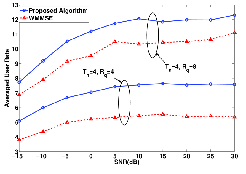
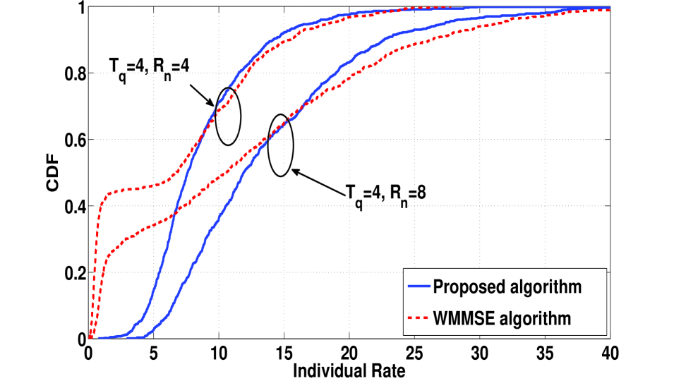
Figure 1: Comparison of the performance of the proposed algorithm and the WMMSE algorithm when the proportional fair utility is used. $N=16$, $Q=7$, users are all located at the cell edges. Left: comparison of the users’ averaged rates. Right: comparison of the CDF of users’ achieved rates.

We first consider a scenario in which the users are all located at the pico cell edges, and one of the pico BSs is congested. In particular, we place half of the users uniformly at the cell edges of BS $1$, which is within $d_{1,n}\in[90,~{}100]$ meters. We place the rest of the users randomly at the cell edges of other pico BSs. For the WMMSE algorithm, we let the users associate to the pico BSs with the strongest direct channel (in terms of the 2-norm of the channel matrices). For our proposed algorithm, we place a restriction that the users can only choose their association among the three strongest pico BSs. We initiate our algorithm by assigning the users to their respective strongest pico BSs. Fig. 1 compares the performance of the algorithms when the proportional fairness utility is used, i.e., $f_{n}(R_{n})=\log(R_{n}),\ \forall\ n\in\mathcal{N}$. Each point on this figure is averaged over $100$ randomly generated user positions and channel coefficients. The left panel of Fig. 1 compares the users’ averaged rates achieved by different algorithms. The right panel of Fig. 1 compares the CDF (cumulative distribution function) of the individual rates of the two algorithms when $\mbox{SNR}=30\mbox{dB}$. Fig. 1 shows that if the user-BS assignment is allowed to be optimized, the proposed algorithm can achieve a substantially higher spectrum efficiency and fairer rate allocation, as compared to the case when the user-BS assignment is fixed. This is reasonable since assigning weak users to less congested BSs (rather than the closest BSs) effectively reduces the interference level (hence the congestion level) of the congested BS. In this way, both user fairness and the spectral efficiency of the entire network are enhanced.

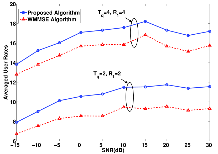
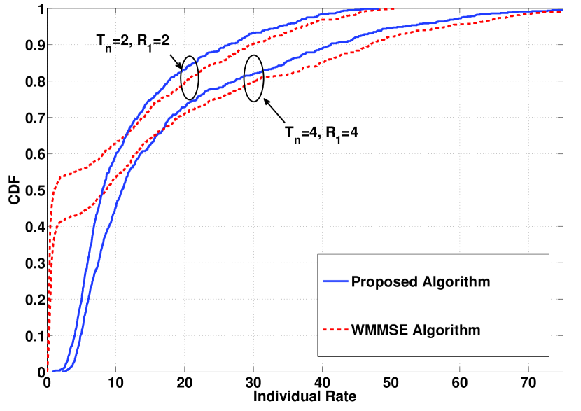
Figure 2: Comparison of the performance of the proposed algorithm and the WMMSE algorithm in a HetNet with different BS capabilities. The proportional fair utility is used. $N=16$, $Q=7$. Half of the users are uniformly distributed in cell $1$, all other users are uniformly distributed in other cells. Three neighboring BSs have $10$ receiving antennas, and all other BSs have the same number of antennas as BS $1$ (which is either $2$ or $4$). Left: comparison of the users’ averaged rates. Right: comparison of the CDF of users’ achieved rates.

To highlight the load balancing capability of the proposed algorithm, we next consider a scenario in a HetNet where the pico BSs have different capabilities. Specifically, three out of the six neighboring pico BSs of BS 1 have $10$ receive antennas, and all other pico BSs (including BS $1$) have fewer receive antennas. Half of the users are uniformly located in cell $1$ (which is within $d_{1,n}\in[20,~{}100]$ meters) and the rest of the users are uniformly located in other cells ($d_{q,n}\in[20,~{}100]$ meters, $q\neq 1$). Again we use the proportional fairness utility function, and the proposed algorithm compares favorably with the WMMSE algorithm. See Fig. 2.

Interestingly, by using the proposed joint BS association and linear precoder optimization algorithm, the “cell breathing” phenomenon [20] can be observed. This phenomenon refers to the desirable load balancing property of a network: when a cell is congested, it contracts and the cell edge users automatically switch to adjacent cells. See Fig. 3 for an illustration.

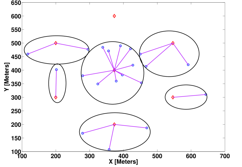
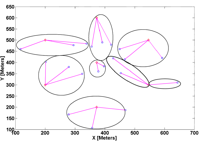
Figure 3: Illustration of the cell breathing phenomenon. $Q=7$, $N=20$, $R_{n}=4$, $T_{q}=4$, proportional fair utility is used. In the figures, the diamonds denote the BSs, the dots denote the users, and the lines indicate associations. Left: user-BS assignment in which users are associated to the BS with the strongest channel magnitude in terms of 2-norm. Right: user-BS assignment generated by the proposed algorithm.

VI Conclusion

In this paper, we consider the joint design of the user-BS assignment and the users’ linear precoder in a multicell heterogeneous network. By a careful user-BS association, users in a hot spot can avoid congesting the nearest BS or causing excessive interference to each other. Unfortunately the overall joint optimization problem is shown to be computationally intractable. To find a high quality locally optimal solution, we propose an efficient and low-complexity algorithm using a game theoretic formulation. The effectiveness of the proposed algorithm is demonstrated via numerical simulations which show substantially improved spectrum efficiency and fairness provisioning. A drawback of this algorithm is the fact that it requires the exact knowledge of channel state information (CSI). An important issue worth investigating is to what extent we can use inexact channel state information or just use the long-term channel statistics in place of the CSI. Another interesting issue is to incorporate the users’ quality of service constraints in the problem formulation.

Appendix A Proof of Theorem 1

Proof:

Given $M$ disjunctive clauses $C_{1},\cdots,C_{M}$ defined on $N$ Boolean variables $X_{1}\cdots,X_{N}$, i.e., $C_{m}=t_{1}\vee t_{2}\vee t_{3}$ with $t_{i}\in\{X_{1},\cdots,X_{N},\bar{X}_{1},\cdots,\bar{X}_{N}\}$, the 3-SAT problem is to check whether there exists a truth assignment for the Boolean variables such that all clauses are satisfied (i.e., each clause evaluates to $1$) simultaneously. Let $\pi(C_{m},i)$ denote the $i^{th}$ term of the clause $C_{m}$, and let $\mathcal{I}(t)$ denote the index of a term $t$’s corresponding variable. For example if $C_{m}=\bar{X}_{1}\vee\bar{X}_{2}\vee X_{4}$, then $\pi(C_{m},1)=\bar{X}_{1}$, and $\mathcal{I}(\pi(C_{m},3))=4$.

Given any 3-SAT problem with $M$ disjunctive clauses and $N$ variables, we construct an instance of multiple BS multi-user uplink network with $3M+N$ BSs and $M+2N$ users. Let $T_{n}=R_{q}=1$, $\sigma^{2}_{q}=1$, $\bar{p}_{n}=1$ and $w_{n}=1$, for all $q,n$. Let $h_{q,n}$ denote the channel coefficient between user $n$ and BS $q$. For each clause $C_{m}$, we construct $3$ clause BSs $\{c^{1}_{m},c^{2}_{m},c^{3}_{m}\}$, and construct $1$ clause user denoted as user $C_{m}$. For each variable $X_{n}$, we construct $1$ variable BS denoted as $x_{n}$, and construct $2$ variable users denoted as $\bar{X}_{n},X_{n}$. The channel coefficients are specified as follows. The clause user $C_{m}$ has nonzero channels only to the clause BSs $\{c^{i}_{m}\}_{i=1}^{3}$. The variable user $X_{n}$ has nonzero channels only to the variable BS $x_{n}$ and the clause BS $C^{i}_{m}$ that satisfies $\bar{X}_{n}=\pi(C_{m},i)$. Similarly, the user $\bar{X}_{n}$ has nonzero channels to the variable BS $x_{n}$ and the clause BS $C^{i}_{m}$ that satisfies ${X}_{n}=\pi(C_{m},i)$. Specifically, the channel coefficients are designed as:

$$h_{q,C_{m}} =\left\{\begin{array}[]{ll}\sqrt{7},&q\in\{c^{1}_{m},c^{2}_{m},c^{3}_{m}\},\\ 0,&q\notin\{c^{1}_{m},c^{2}_{m},c^{3}_{m}\}.\end{array}\right.$$ (42)

$$h_{q,X_{n}} =\left\{\begin{array}[]{ll}\sqrt{7},&q=x_{n},\\ 1,&q=c^{i}_{m},~{}\textrm{and}~{}\pi(C_{m},i)=\bar{X}_{n},\\ 0,&\textrm{otherwise}.\end{array}\right.$$ (46)

$$h_{q,\bar{X}_{n}} =\left\{\begin{array}[]{ll}\sqrt{7},&q=x_{n},\\ 1,&q=c^{i}_{m},~{}\textrm{and}~{}\pi(C_{m},i)={X}_{n},\\ 0,&\textrm{otherwise}.\end{array}\right.$$ (50)

To illustrate, for a given clause $C_{m}=X_{1}\vee\bar{X}_{2}\vee X_{3}$, we construct the network shown in Fig. 5.

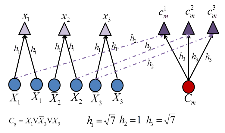
Figure 4: Construction of the network for clause $C_{m}=X_{1}\vee\bar{X}_{2}\vee X_{3}$.

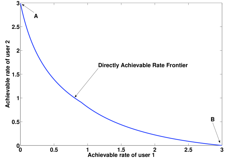
Figure 5: Achievable rate frontier of two-user single channel interference channel when all the direct and cross talk channel coefficients are set to be $\sqrt{7}$.

Our claim is that the 3-SAT problem will be satisfied if and only if the network we constructed achieves a total sum rate of at least $3(M+N)$.

Suppose that the 3-SAT problem is satisfied, then we perform the following assignment: 1) If $X_{n}=1$, assign the corresponding variable user $X_{n}$ to BS $x_{n}$. Otherwise, assign user $\bar{X}_{n}$ to BS $x_{n}$. 2) for each clause $C_{m}$, pick an index $i^{*}_{m}\in\{1,2,3\}$ such that $\pi(C_{m},i^{*}_{m})=1$ (note that because the 3-SAT problem is satisfied, we can always do so). Assign the clause user $C_{m}$ to the clause BS $c^{i^{*}_{m}}_{m}$. We claim that by the above user-BS assignment, and by letting all the assigned users transmit with full power, the overall sum rate achieved is $3(M+N)$. To argue this claim, we first note that there is a single user in the variable user pair $\bar{X}_{n},X_{n}$ that transmits with full power to BS $x_{n}$. Thus each variable BS $x_{n}$ is free of multiuser interference and obtains a rate of $\log(1+\frac{7}{1})=3$. We then consider an arbitrary clause $C_{m}$, and pick a term $t$ that evaluates to $1$, i.e., $t=\pi(C_{m},i^{*}_{m})$. According to our assignment scheme, user $\bar{t}$ does not transmit while user $t$ transmits with full power. By our construction of the channel in (42)–(50), the only variable user that has nonzero channel to the clause BS $c^{i^{*}_{m}}_{m}$ is user $\bar{t}$. Since user $\bar{t}$ does not transmit, then the clause user $C_{m}$ can transmit to clause BS $c^{i^{*}_{m}}_{m}$ free of interference. Consequently it obtains a rate of $\log(1+\frac{7}{1})=3$. In summary, each variable BS is able to achieve a rate of $3$, while each set of three clause BSs $\{c_{m}^{1},c_{m}^{2},c_{m}^{3}\}$ obtains a total rate of $3$. Thus the total system sum rate is $3(M+N)$.

Conversely, suppose the network achieves a total rate of $3(M+N)$, we argue that the corresponding 3-SAT problem must be satisfied. We show this direction by three steps.

Step 1) We first claim that for any variable BS $x_{n}$, its maximum achievable sum rate is obtained when a single variable user, $X_{n}$ or $\bar{X}_{n}$, transmits to it using full power, while the remaining user does not transmit. Let $p_{X_{n}}$ and $p_{\bar{X}_{n}}$ denote the transmission power of user $X_{n}$ and $\bar{X}_{n}$, respectively. The rate region of this uplink channel when the interference is treated as noise can be expressed as

$${\mathcal{R}}=\{(R_{\bar{X}_{n}}(p_{{X}_{n}},p_{\bar{X}_{n}}),R_{X_{n}}(p_{{X}_{n}},p_{\bar{X}_{n}})):0\leq p_{X_{n}}\leq 1,0\leq p_{\bar{X}_{n}}\leq 1\}$$

where $$R_{{X}_{n}}(p_{{X}_{n}},p_{\bar{X}_{n}})=\log\left(1+\frac{p_{{X}_{n}}|h_{x_{n},{X}_{n}}|^{2}}{1+p_{\bar{X}_{n}}|h_{x_{n},\bar{X}_{n}}|^{2}}\right)$$

$$R_{\bar{X}_{n}}(p_{{X}_{n}},p_{\bar{X}_{n}})=\log\left(1+\frac{p_{\bar{X}_{n}}|h_{x_{n},\bar{X}_{n}}|^{2}}{1+p_{X_{n}}|h_{x_{n},X_{n}}|^{2}}\right)$$ (51)

with the channel coefficients given as $h_{x_{n},\bar{X}_{n}}=h_{x_{n},{X}_{n}}=\sqrt{7}$. In [38], Charafeddine and Paulraj derived a complete characterization of this rate region (without time-sharing operation). This region (plotted in Fig. 5) asserts that the sum rate maximum point can be achieved only if a single user transmits using its full power (at point A or B).

Step 2) We then argue that a variable user should never be assigned to any clause BS at the sum-rate optimal solution. To see this, consider an arbitrary $C_{m}$ and an arbitrary $i\in\{1,2,3\}$, let $t=\pi(C_{m},i)$. Suppose at the optimal solution user $t$ transmits to BS $c^{i}_{m}$, then it can obtain a maximum rate of $\log(1+\frac{1}{1})=1$. If BS $x_{\mathcal{I}(t)}$ has no associated user at the optimal solution, then the same user $t$ can switch to BS $x_{\mathcal{I}(t)}$ and obtain a rate increase of $\log(1+\frac{7}{1})-\log(1+1)=2$. This is a contradiction to the optimality of the solution. Consequently BS $x_{\mathcal{I}(t)}$ must have user $\bar{t}$ associated to it. In this case, the maximum sum rate that user $t$ and $\bar{t}$ can obtain is the optimal solution for the following problem

$$~{}\max_{0\leq p_{t},p_{\bar{t}}\leq 1}\log\left(1+\frac{7p_{\bar{t}}}{1+7p_{{t}}}\right)+\log\left(1+p_{t}\right).$$

Clearly at the optimal $p_{\bar{t}}=1$, and the tuple $(p_{t},p_{\bar{t}})=(0,1)$ is a feasible solution to the above problem with an objective value $\log(1+\frac{7}{1})=3$. We then argue that $(p_{t},p_{\bar{t}})=(0,1)$ is in fact the optimal solution to this optimization problem. Specifically, we will show that the following is true

$$\log\left(1+\frac{7}{1+7p_{t}}\right)+\log\left(1+p_{t}\right)<\log(1+7),~{}\forall~{}0<p_{t}\leq 1.$$ (52)

Equivalent we show the following inequality

$$f(p_{t})\triangleq\left(1+\frac{7}{1+7p_{t}}\right)(1+p_{t})<8,~{}\forall~{}0<p_{t}\leq 1.$$ (53)

Note that $\frac{df(p_{t})}{dp_{t}}=1-\frac{42}{(1+7p_{t})^{2}}$. So when $p_{t}\in[0,\frac{\sqrt{42}-1}{7}]$, the slope of $f(p_{t})$ is negative, and the functional value of $f(p_{t})$ is strictly decreasing. when $p_{t}\in(\frac{\sqrt{42}-1}{7},1]$, the functional value of $f(p_{t})$ is strictly increasing. Combining with the fact that $f(0)=8$ and $f(1)=2+\frac{7}{4}<8$, we have that $f(p_{t})<8$ for all $0<p_{x_{n}}\leq 1$. In summary, a variable user never transmits to any clause BS at the sum rate optimal solution.

Step 3) The third step is to show that any clause $BS$ tuple $\{c^{1}_{m},c^{2}_{m},c^{3}_{m}\}$ can at most obtain a rate of $\log(1+\frac{7}{1})=3$ at the sum rate optimal point. This step is trivial as the only candidate that can select and transmit to clause BSs $\{c^{i}_{m}\}_{i=1}^{3}$ is the clause user $C_{m}$. When there is no interference, the maximum rate user $C_{m}$ (and equivalently the set of BSs $\{c^{i}_{m}\}_{i=1}^{3}$) can get is $\log(1+7)=3$. Note that this maximum rate can be achieved only when at least one of these clause BSs does not experience interference from the variable users.

Step 2-3 together imply that each variable BS and each clause BS tuple $\{c^{i}_{m}\}_{i=1}^{3}$ are able to achieve a rate at most $3$ at sum rate optimal point. As a result, in order to achieve a system rate of $3(M+N)$, each of them must achieve a rate that exactly equals to $3$. From Step 3, for any clause $C_{m}$, if a BS tuple $\{c^{i}_{m}\}_{i=1}^{3}$ achieves a throughput of $3$, then it is only possible that there exists a index $i^{*}_{m}$ and a user $t^{*}_{m}=C(m,i^{*}_{m})$ such that user $\bar{t^{*}}_{m}$ does not transmit. Set the terms $t^{*}_{m}=1$ for each clause $m=1,\cdots,M$. This assignment ensures that every clause $C_{m}$ contains at least one term that is assigned to $1$. Consequently, the 3-SAT problem is satisfied.

Since the above construction only involves universal constants, the joint linear precoder design and base station selection problem (SYS) is strongly NP-hard. The proof is complete. ∎

Appendix B Proof of Lemma 1

Proof:

We prove this claim by contradiction. Suppose the contrary, that $\alpha_{n}\bigg{(}\sum_{i=1}^{T_{n}}\log\big{(}\frac{c[\Delta_{n}]^{2}_{i,i}}{1-\zeta^{*}_{i}(c)}\big{)}\bigg{)}>c$ and $c^{*}\leq c$. Define $s^{*}_{i}(c)\triangleq\big{[}c-\frac{1}{[\Delta_{n}]^{2}_{i,i}}\big{]}^{+}$. Define the following two sets

$$\mathcal{I}(c) \triangleq\left\{i\mid s^{*}_{i}(c)=0\right\},\ \overline{\mathcal{I}}(c)\triangleq\left\{i\mid s^{*}_{i}(c)>0\right\}.$$

From the definition $s^{*}_{i}(c)=\big{[}c-\frac{1}{[\Delta_{n}]^{2}_{i,i}}\big{]}^{+},\ \zeta^{*}_{i}(c)=\big{[}1-c[\Delta_{n}]^{2}_{i,i}\big{]}^{+}$, we have

$$\alpha_{n}\left(\sum_{i=1}^{T_{n}}\log\left(\frac{c[\Delta_{n}]^{2}_{i,i}}{1-\zeta^{*}_{i}(c)}\right)\right) =\alpha_{n}\left(\sum_{i\in\overline{\mathcal{I}}(c)}\log\left(\frac{c[\Delta_{n}]^{2}_{i,i}}{1-\zeta^{*}_{i}(c)}\right)\right)$$

$$=\alpha_{n}\left(\sum_{i\in\overline{\mathcal{I}}(c)}\log\left(c[\Delta_{n}]^{2}_{i,i}\right)\right).$$

Note that if $c^{*}\leq c$, we have $\overline{\mathcal{I}}(c^{*})\subseteq\overline{\mathcal{I}}(c),~{}\mathcal{I}(c^{*})\supseteq{\mathcal{I}}(c)$. This together with the fact that $c^{*}\leq c$ imply

$$\sum_{i\in\overline{\mathcal{I}}(c)}\log\left(c[\Delta_{n}]^{2}_{i,i}\right)\geq\sum_{i\in\overline{\mathcal{I}}(c^{*})}\log\left(c^{*}[\Delta_{n}]^{2}_{i,i}\right).$$

Since, as the derivative of a concave utility function, the function $\alpha_{n}(\cdot)$ is monotonically decreasing, we obtain

$$\alpha_{n}\left(\sum_{i=1}^{T_{n}}\log\left(\frac{c^{*}[\Delta_{n}]^{2}_{i,i}}{1-\zeta^{*}_{i}(c^{*})}\right)\right)=\alpha_{n}\left(\sum_{i\in\overline{\mathcal{I}}(c^{*})}\log\left(c^{*}[\Delta_{n}]^{2}_{i,i}\right)\right)$$

$$\geq\alpha_{n}\left(\sum_{i\in\overline{\mathcal{I}}(c)}\log\left(c[\Delta_{n}]^{2}_{i,i}\right)\right)>c\geq c^{*}.$$

This is a contradiction to the optimality condition that

$$\alpha_{n}\left(\sum_{i=1}^{T_{n}}\log\left(\frac{c^{*}[\Delta_{n}]^{2}_{i,i}}{1-\zeta^{*}_{i}(c^{*})}\right)\right)=c^{*}.$$

Thus we conclude that any fixed $c$, if $\alpha_{n}\bigg{(}\sum_{i=1}^{T_{n}}\log\big{(}\frac{c[\Delta_{n}]^{2}_{i,i}}{1-\zeta^{*}_{i}(c)}\big{)}\bigg{)}>c$, then $c^{*}>c$.

The other direction can be shown similarly. ∎

Appendix C Proof of Lemma 2

We show that the function $-{\mbox{{Tr}}}\left[\mathbf{E}^{-1}_{m}(\widehat{\mathbf{S}})\mathbf{E}_{m}(\mathbf{S}_{n},{\mathbf{S}}_{-n})\right]$ is convex in $\mathbf{S}_{n}$. Let

$$g_{m}(\mathbf{S}_{n}) \triangleq{\mbox{{Tr}}}\left[\mathbf{E}^{-1}_{m}(\widehat{\mathbf{S}})({\mathbf{S}}_{m}^{\frac{1}{2}})^{H}\mathbf{H}^{H}_{\mathbf{a}_{m},m}\mathbf{G}_{m}^{-1}(\mathbf{S})\mathbf{H}_{\mathbf{a}_{m},m}{\mathbf{S}}^{\frac{1}{2}}_{m}\right].$$

From [33], we see that in order to prove that $g_{m}(\mathbf{S}_{n})$ is convex in $\mathbf{S}_{n}$, it is sufficient to prove that $g_{m}(\mathbf{S}_{n}+t\mathbf{D})$ is convex in the scalar variable $t$, for any fixed direction $\mathbf{D}\in\mathbb{S}^{T_{n}}$ as long as $\mathbf{S}_{n}+t\mathbf{D}\in\mathbb{S}^{T_{n}}_{+}$. In what follows, we will show that for all $\mathbf{D}\in\mathbb{S}^{T_{n}}$ that satisfies $\mathbf{S}_{n}+t\mathbf{D}\succeq 0$, we have $\frac{\partial^{2}g(\mathbf{S}_{n}+t\mathbf{D})}{\partial t^{2}}\geq 0$.

To proceed, we make the following definitions

$$\mathbf{B} \triangleq\mathbf{H}_{\mathbf{a}_{n},n}\mathbf{D}\mathbf{H}^{H}_{\mathbf{a}_{n},n},$$

$$\mathbf{G}_{m}(t) \triangleq\sigma^{2}_{\mathbf{a}_{n}}\mathbf{I}+\sum_{l=1}^{N}\mathbf{H}_{\mathbf{a}_{n},l}\mathbf{S}_{l}\mathbf{H}^{H}_{\mathbf{a}_{n},l}+t\mathbf{H}_{\mathbf{a}_{n},n}\mathbf{D}\mathbf{H}^{H}_{\mathbf{a}_{n},n}.$$

The first and second order derivatives of $g_{m}(\mathbf{S}_{n}+t\mathbf{D})$ with respect to $t$ can be expressed as

$$\frac{\partial g_{m}(\mathbf{S}_{n}+t\mathbf{D})}{\partial t} =-{\mbox{{Tr}}}\left[\mathbf{E}^{-1}_{m}(\widehat{\mathbf{S}})(\mathbf{S}_{m}^{\frac{1}{2}})^{H}\mathbf{H}^{H}_{\mathbf{a}_{m},m}\mathbf{G}_{m}^{-1}(t)\mathbf{B}\mathbf{G}_{m}^{-1}(t)\mathbf{H}_{\mathbf{a}_{m},m}\mathbf{S}^{\frac{1}{2}}_{m}\right]$$

$$\frac{\partial^{2}g_{m}(\mathbf{S}_{n}+t\mathbf{D})}{\partial t^{2}} =2{\mbox{{Tr}}}\left[\mathbf{E}^{-1}_{m}(\widehat{\mathbf{S}})(\mathbf{S}_{m}^{\frac{1}{2}})^{H}\mathbf{H}^{H}_{\mathbf{a}_{m},m}\mathbf{G}_{m}^{-1}(t)\mathbf{B}\mathbf{G}_{m}^{-1}(t)\mathbf{B}\mathbf{G}_{m}^{-1}(t)\mathbf{H}_{\mathbf{a}_{m},m}\mathbf{S}^{\frac{1}{2}}_{m}\right].$$

The fact that $\mathbf{S}_{n}+t\mathbf{D}\succ 0$ ensures $\mathbf{G}_{m}(t)\succ 0$, which further implies

$$(\mathbf{S}_{n}^{\frac{1}{2}})^{H}\mathbf{H}^{H}_{\mathbf{a}_{n},n}\mathbf{G}_{m}^{-1}(t)\mathbf{B}\mathbf{G}_{m}^{-1}(t)\mathbf{B}\mathbf{G}_{m}^{-1}(t)\mathbf{H}_{\mathbf{a}_{n},n}\mathbf{S}^{\frac{1}{2}}_{n}\succeq 0.$$

Combining with the fact that $\mathbf{E}^{-1}_{m}(\widehat{\mathbf{S}})\succ 0$, we conclude that $\frac{\partial^{2}g_{m}(\mathbf{S}_{n}+t\mathbf{D})}{\partial t^{2}}\geq 0$.

Appendix D Proof of Proposition 2

Proof:

We first write an equivalent form of (33) (note that we have defined $\widehat{\mathbf{J}}=(\widehat{\mathbf{S}},\widehat{\mathbf{a}})$)

$$\bar{U}_{n}\left({\mathbf{J}}_{n},\widehat{\mathbf{J}}_{-n},\mathbf{T}_{n}(\widehat{\mathbf{J}})\right)-\bar{U}_{n}\left(\widehat{\mathbf{J}}_{n},\widehat{\mathbf{J}}_{-n},\mathbf{T}_{n}(\widehat{\mathbf{J}})\right)$$

$$= \left[\bar{U}_{n}\left(({\mathbf{S}}_{n},\mathbf{a}_{n}),\widehat{\mathbf{J}}_{-n},\mathbf{T}_{n}(\widehat{\mathbf{S}},\widehat{\mathbf{a}})\right)-\bar{U}_{n}\left((\widehat{\mathbf{S}}_{n},\mathbf{a}_{n}),\widehat{\mathbf{J}}_{-n},\mathbf{T}_{n}(\widehat{\mathbf{S}},[\mathbf{a}_{n},\widehat{\mathbf{a}}_{-n}])\right)\right]$$

$$+\left[\bar{U}_{n}\left((\widehat{\mathbf{S}}_{n},\mathbf{a}_{n}),\widehat{\mathbf{J}}_{-n},\mathbf{T}_{n}(\widehat{\mathbf{S}},[\mathbf{a}_{n},\widehat{\mathbf{a}}_{-n}])\right)-\bar{U}_{n}\left((\widehat{\mathbf{S}}_{n},\widehat{\mathbf{a}}_{n}),\widehat{\mathbf{J}}_{-n},\mathbf{T}_{n}(\widehat{\mathbf{S}},\widehat{\mathbf{a}})\right)\right].$$ (54)

We show that the following identities are true

$$R_{m}((\widehat{\mathbf{S}}_{n},\mathbf{a}_{n}),\widehat{\mathbf{J}}_{-n})=R_{m}((\widehat{\mathbf{S}}_{n},\widehat{\mathbf{a}}_{n}),\widehat{\mathbf{J}}_{-n}),~{}\forall~{}m\neq n$$ (55)

$$\mathbf{T}_{q,n}(\widehat{\mathbf{S}},\widehat{\mathbf{a}})=\mathbf{T}_{q,n}(\widehat{\mathbf{S}},[\mathbf{a}_{n},\widehat{\mathbf{a}}_{-n}]),~{}\forall~{}q\in\mathcal{Q}.$$ (56)

This set of equations implies that if user $n$ unilaterally switches from BS $\widehat{\mathbf{a}}_{n}$ to $\mathbf{a}_{n}$ but keeps its covariance matrix unchanged, then all other users’ transmission rates as well as the prices charged for user $n$ remain the same.

Identity (55) is straightforward as the interference at user $m$’ receiver caused by user $n$ is unchanged as long as user $n$’s transmit covariance matrix remains to be $\widehat{\mathbf{S}}_{n}$.

To verify (56), we first recall that the prices are defined as follows

$$\mathbf{T}_{q,n}(\widehat{\mathbf{S}},\widehat{\mathbf{a}}) =-\sum_{m\in\mathcal{N}_{q}(\widehat{\mathbf{a}})\setminus n}\frac{\partial f_{m}(R_{m})}{\partial R_{m}}\bigg{|}_{R_{m}=R_{m}(\widehat{\mathbf{S}})}\mathbf{H}^{H}_{q,n}{\mathbf{C}}_{m}^{-1}(\widehat{\mathbf{S}}_{-m})\left(\mathbf{I}_{R_{q}}+\mathbf{H}_{q,m}{\widehat{\mathbf{S}}}_{m}\mathbf{H}^{H}_{q,m}{\mathbf{C}}_{m}^{-1}(\widehat{\mathbf{S}}_{-m})\right)^{-1}$$

$$\quad\times\mathbf{H}_{q,m}\widehat{\mathbf{S}}_{m}\mathbf{H}^{H}_{q,m}{\mathbf{C}}_{m}^{-1}(\widehat{\mathbf{S}}_{-m})\mathbf{H}_{q,n}.$$ (57)

Take any BS $q$ that satisfies $q\neq\mathbf{a}_{n}$ and $q\neq\widehat{\mathbf{a}}_{n}$. Clearly we have $\{m:m\in\mathcal{N}_{q}(\widehat{\mathbf{a}}),m\neq n\}=\{m:m\in\mathcal{N}_{q}([\mathbf{a}_{n},\widehat{\mathbf{a}}_{-n}]),m\neq n\}$. For BS $q=\widehat{\mathbf{a}}_{n}$ or $q={\mathbf{a}}_{n}$, although user $n$ has changed its association, the other users’ associations remain the same. That is, we again have $\{m:m\in\mathcal{N}_{q}(\widehat{\mathbf{a}}),m\neq n\}=\{m:m\in\mathcal{N}_{q}([\mathbf{a}_{n},\widehat{\mathbf{a}}_{-n}]),m\neq n\}$. Combining the above two observations with the fact that the transmit covariances $\widehat{\mathbf{S}}$ of all the users remain the same, we conclude that $\mathbf{T}_{q,n}(\widehat{\mathbf{S}},\widehat{\mathbf{a}})=\mathbf{T}_{q,n}(\widehat{\mathbf{S}},[\mathbf{a}_{n},\widehat{\mathbf{a}}_{-n}])$, for all $q\in\mathcal{Q}$. This proves (56).

Now using (56), the first difference in (54) becomes

$$\bar{U}_{n}\left(({\mathbf{S}}_{n},\mathbf{a}_{n}),\widehat{\mathbf{J}}_{-n},\mathbf{T}_{n}(\widehat{\mathbf{S}},\widehat{\mathbf{a}})\right)-\bar{U}_{n}\left((\widehat{\mathbf{S}}_{n},\mathbf{a}_{n}),\widehat{\mathbf{J}}_{-n},\mathbf{T}_{n}(\widehat{\mathbf{S}},[\mathbf{a}_{n},\widehat{\mathbf{a}}_{-n}])\right)$$

$$=\left(\bar{U}_{n}\left(({\mathbf{S}}_{n},\mathbf{a}_{n}),\widehat{\mathbf{J}}_{-n},\mathbf{T}_{n}(\widehat{\mathbf{S}},[\mathbf{a}_{n},\widehat{\mathbf{a}}_{-n}])\right)-\bar{U}_{n}\left((\widehat{\mathbf{S}}_{n},\mathbf{a}_{n}),\widehat{\mathbf{J}}_{-n},\mathbf{T}_{n}(\widehat{\mathbf{S}},[\mathbf{a}_{n},\widehat{\mathbf{a}}_{-n}])\right)\right)$$

$$\stackrel{{\scriptstyle\mbox{\footnotesize(i)}}}{{\leq}}f\left(({\mathbf{S}}_{n},\mathbf{a}_{n}),\widehat{\mathbf{J}}_{-n}\right)-f\left((\widehat{\mathbf{S}}_{n},\mathbf{a}_{n}),\widehat{\mathbf{J}}_{-n}\right).$$ (58)

where the inequality (i) is due to (32), which states that for a fixed system association profile ($[\mathbf{a}_{n},\widehat{\mathbf{a}}_{-n}]$ in this case), the user $n$’s increase of utility induced by unilateral change of its transmit covariance is upper bounded by the increase of the system sum utility. The second difference in (54) becomes

$$\bar{U}_{n}\left((\widehat{\mathbf{S}}_{n},\mathbf{a}_{n}),\widehat{\mathbf{J}}_{-n},\mathbf{T}_{n}(\widehat{\mathbf{S}},[\mathbf{a}_{n},\widehat{\mathbf{a}}_{-n}])\right)-\bar{U}_{n}\left((\widehat{\mathbf{S}}_{n},\widehat{\mathbf{a}}_{n}),\widehat{\mathbf{J}}_{-n},\mathbf{T}_{n}(\widehat{\mathbf{S}},\widehat{\mathbf{a}})\right)$$

$$=f_{n}\left(R_{n}((\widehat{\mathbf{S}}_{n},\mathbf{a}_{n}),\widehat{\mathbf{J}}_{-n})\right)-\mbox{Tr}\left[\mathbf{T}_{n}(\widehat{\mathbf{S}},[\mathbf{a}_{n},\widehat{\mathbf{a}}_{-n}])\widehat{\mathbf{S}}_{n}\right]-f_{n}\left(R_{n}((\widehat{\mathbf{S}}_{n},\widehat{\mathbf{a}}_{n}),\widehat{\mathbf{J}}_{-n})\right)+\mbox{Tr}\left[\mathbf{T}_{n}(\widehat{\mathbf{S}},\widehat{\mathbf{a}})\widehat{\mathbf{S}}_{n}\right]$$

$$\stackrel{{\scriptstyle\rm{\footnotesize(i)}}}{{=}}f_{n}\left(R_{n}((\widehat{\mathbf{S}}_{n},\mathbf{a}_{n}),\widehat{\mathbf{J}}_{-n})\right)-f_{n}\left(R_{n}((\widehat{\mathbf{S}}_{n},\widehat{\mathbf{a}}_{n}),\widehat{\mathbf{J}}_{-n})\right)$$

$$\stackrel{{\scriptstyle\mbox{\footnotesize(ii)}}}{{=}}\sum_{m=1}^{N}f_{m}\left(R_{m}((\widehat{\mathbf{S}}_{m},\mathbf{a}_{m}),\widehat{\mathbf{J}}_{-m})\right)-f_{m}\left(R_{m}((\widehat{\mathbf{S}}_{m},\widehat{\mathbf{a}}_{m}),\widehat{\mathbf{J}}_{-m})\right)=f\left((\widehat{\mathbf{S}}_{n},\mathbf{a}_{n}),\widehat{\mathbf{J}}_{-n}\right)-f\left((\widehat{\mathbf{S}}_{n},\widehat{\mathbf{a}}_{n}),\widehat{\mathbf{J}}_{-n}\right)$$ (59)

where the step $\rm(i)$ follows from (56) and step (ii) is due to (55). Combining (54), (58) and (59), we have that

$$\bar{U}_{n}\left(({\mathbf{S}}_{n},\mathbf{a}_{n}),\widehat{\mathbf{J}}_{-n},\mathbf{T}_{n}(\widehat{\mathbf{S}},\widehat{\mathbf{a}})\right)-\bar{U}_{n}\left((\widehat{\mathbf{S}}_{n},\widehat{\mathbf{a}}_{n}),\widehat{\mathbf{J}}_{-n},\mathbf{T}_{n}(\widehat{\mathbf{S}},\widehat{\mathbf{a}})\right)$$

$$\leq f\left(({\mathbf{S}}_{n},\mathbf{a}_{n}),\widehat{\mathbf{J}}_{-n}\right)-f\left((\widehat{\mathbf{S}}_{n},\widehat{\mathbf{a}}_{n}),\widehat{\mathbf{J}}_{-n}\right).$$ (60)

This proves the claim. ∎

Appendix E Proof of Theorem 4

By the generalized potential property stated in Proposition 2, the sequence $\{f(\mathbf{S}^{t},\mathbf{a}^{t})\}$ is monotonically increasing and converges. Let us denote the limit of this sequence as $f^{*}$.

Let $\mathcal{A}$ be the set of association profiles that appear infinitely often in the sequence $\{\mathbf{a}^{t}\}$. Take any $\mathbf{a}\in\mathcal{A}$, define the subsequence $\{\mathbf{a}^{\tilde{t}_{k}}\}$ of $\{\mathbf{a}^{t}\}$ that satisfies

$$\mathbf{a}^{\tilde{t}_{k}}=\mathbf{a},~{}\textrm{and~{}}\mathbf{a}^{m}\neq\mathbf{a},~{}\forall~{}m\in(\tilde{t}_{k},\tilde{t}_{k+1}).$$

Clearly the sequence $\{f(\mathbf{S}^{\tilde{t}_{k}},\mathbf{a}^{\tilde{t}_{k}})\}_{k}$ is also increasing and converges to $f^{*}$. Let $\mathbf{S}^{*}$ be a limit point of $\{\mathbf{S}^{\tilde{t}_{k}}\}$. Take a further subsequence $\{\mathbf{a}^{{t}_{k}}\}$ of $\{\mathbf{a}^{\tilde{t}_{k}}\}$ such that $\lim_{k\to\infty}\mathbf{S}^{{t}_{k}}=\mathbf{S}^{*}$. Due to the fact that $\mathbf{T}_{n}(\cdot)$ is a continuous function in $\mathbf{S}$, the subsequence $\{\mathbf{T}^{t_{k}}_{n}(\mathbf{S}^{{t}_{k}})\}$ must be convergent for all $n$. Let $\mathbf{T}_{n}^{*}=\mathbf{T}_{n}(\mathbf{S}^{*})$ for all $n$. We wish to show that $(\mathbf{S}^{*},\mathbf{a},\mathbf{T}^{*})$ is a NE of the game $\mathcal{G}^{J}$. The desired result will be shown in two steps.

S1) $\bar{U}_{n}(\mathbf{S}^{*},\mathbf{a},\mathbf{T}^{*}_{n})\geq\bar{U}_{n}([\mathbf{S}_{n},\mathbf{S}_{-n}^{*}],[{\mathbf{a}}_{n},\mathbf{a}_{-n}],\mathbf{T}^{*}_{n}),~{}\forall~{}\mathbf{S}_{n}\in\mathcal{F}_{n}\ \forall n\in\mathcal{N}.$

S2) $\bar{U}_{n}(\mathbf{S}^{*},\mathbf{a},\mathbf{T}^{*}_{n})\geq\bar{U}_{n}([\mathbf{S}_{n},\mathbf{S}_{-n}^{*}],[\widehat{\mathbf{a}}_{n},\mathbf{a}_{-n}],\mathbf{T}^{*}_{n}),~{}\forall~{}\widehat{\mathbf{a}}_{n}\neq\mathbf{a}_{n},~{}\forall~{}\mathbf{S}_{n}\in\mathcal{F}_{n}.\ \forall n\in\mathcal{N}$.

Without loss of generality (by possibly restricting to a further subsequence), we can assume that at time instance $t_{k}+1$, it is user $1$’s turn to act.

Step 1) Let $(\mathbf{S}^{*}_{1})^{t_{k}}$ be the (unique) solution to the problem $\max_{\mathbf{S}_{1}\in\mathcal{F}_{1}}\bar{U}_{1}(\mathbf{S}_{1},\mathbf{S}_{-1}^{t_{k}},\mathbf{a}^{t_{k}},\mathbf{T}^{t_{k}}_{1})$. To show S1), it is sufficient to show that $\lim_{k\to\infty}\|(\mathbf{S}^{*})_{1}^{t_{k}}-\mathbf{S}_{1}^{t_{k}}\|=0$. Due to the strict concavity of $\bar{U}_{1}(\mathbf{S}_{1},\mathbf{S}_{-1},\mathbf{a},\mathbf{T}_{1})$ in $\mathbf{S}_{1}$, and use the definition of $(\mathbf{S}^{*}_{1})^{t_{k}}$, we have:

$$\bar{U}_{1}\left((\mathbf{S}_{1}^{*})^{t_{k}},\mathbf{S}^{t_{k}}_{-1},\mathbf{a}^{t_{k}},\mathbf{T}_{1}^{t_{k}}\right) >\bar{U}_{1}\left(\mathbf{S}_{1}+t((\mathbf{S}_{1}^{*})^{t_{k}}-\mathbf{S}_{1}),\mathbf{S}^{t_{k}}_{-1},\mathbf{a}^{t_{k}},\mathbf{T}_{1}^{t_{k}}\right),~{}\forall~{}t\in[0,~{}1),~{}\mathbf{S}_{1}\neq(\mathbf{S}^{*}_{1})^{t_{k}}.$$ (61)

We will show that $\lim_{k\to\infty}(\mathbf{S}^{*}_{1})^{t_{k}}-\mathbf{S}_{1}^{t_{k}}=0$. The proof is along the lines of that of [39, Proposition 2.7.1], but with some important modifications, due to the lack of concavity/convexity of the function $f(\cdot)$ with $\mathbf{S}_{1}$. Suppose $\{(\mathbf{S}^{*}_{1})^{t_{k}}-\mathbf{S}_{1}^{t_{k}}\}$ does not converge to $0$. Let $\gamma^{t_{k}}\triangleq\|(\mathbf{S}^{*}_{1})^{t_{k}}-\mathbf{S}_{1}^{t_{k}}\|$, then by possibly restricting to a further subsequence of $\{t_{k}\}$, we can find a $\bar{\gamma}>0$ such that $\gamma^{t_{k}}\geq\bar{\gamma},~{}\forall~{}k$. Let $\mathbf{V}_{1}^{t_{k}}=((\mathbf{S}^{*}_{1})^{t_{k}}-\mathbf{S}_{1}^{t_{k}})/\gamma^{t_{k}}$, which is equivalent to $(\mathbf{S}^{*}_{1})^{t_{k}}=\mathbf{S}_{1}^{t_{k}}+\gamma^{t_{k}}\mathbf{V}_{1}^{t_{k}}$. Clearly, $\|\mathbf{V}_{1}^{t_{k}}\|=1$, and by possibly restricting to a further subsequence, we assume that $\mathbf{V}_{1}^{t_{k}}$ converges to $\bar{\mathbf{V}}_{1}$.

Let us fixed some $\epsilon\in(0,1)$. We must have $0<\epsilon\bar{\gamma}<\gamma^{t_{k}}$. So $\mathbf{S}_{1}^{t_{k}}+\epsilon\bar{\gamma}\mathbf{V}_{1}^{t_{k}}$ lies on the line segment joining $\mathbf{S}_{1}^{t_{k}}$ and $\mathbf{S}_{1}^{t_{k}}+{\gamma}^{t_{k}}\mathbf{V}_{1}^{t_{k}}=(\mathbf{S}^{*}_{1})^{t_{k}}$. Since $(\mathbf{S}_{1}^{t_{k}+1},\mathbf{a}_{1}^{t_{k}+1})$ is the solution to user $1$’s utility optimization problem at time $t_{k}+1$, we have (recall that $\mathbf{J}^{t_{k}}_{-1}=(\mathbf{S}_{-1}^{t_{k}},\mathbf{a}_{-1}^{t_{k}})$)

$$\bar{U}_{1}((\mathbf{S}_{1}^{t_{k}+1},\mathbf{a}_{1}^{t_{k}+1}),\mathbf{J}^{t_{k}}_{-1},\mathbf{T}_{1}^{t_{k}})$$

$$\geq\bar{U}_{1}((\mathbf{S}^{*}_{1})^{t_{k}},\mathbf{S}_{-1}^{t_{k}},\mathbf{a}^{t_{k}},\mathbf{T}_{1}^{t_{k}})=\bar{U}_{1}(\mathbf{S}^{t_{k}}_{1}+{\gamma}^{t_{k}}\mathbf{V}^{t_{k}}_{1},\mathbf{S}_{-1}^{t_{k}},\mathbf{a}^{t_{k}},\mathbf{T}_{1}^{t_{k}})$$

$$\geq\bar{U}_{1}(\mathbf{S}^{t_{k}}+\epsilon\bar{\gamma}\mathbf{V}^{t_{k}},\mathbf{S}_{-1}^{t_{k}},\mathbf{a}^{t_{k}},\mathbf{T}_{1}^{t_{k}})\geq\bar{U}_{1}(\mathbf{S}_{1}^{t_{k}},\mathbf{S}_{-1}^{t_{k}},\mathbf{a}^{t_{k}},\mathbf{T}_{1}^{t_{k}}).$$

where the last two steps follow from the concavity of $\bar{U}$ (cf. (61)). Combining the above inequality with (60), we have

$$f((\mathbf{S}_{1}^{t_{k}+1},\mathbf{a}_{1}^{t_{k}+1}),\mathbf{J}^{t_{k}}_{-1})-f((\mathbf{S}_{1}^{t_{k}},\mathbf{a}_{1}^{t_{k}}),\mathbf{J}^{t_{k}}_{-1})$$

$$\geq\bar{U}_{1}((\mathbf{S}_{1}^{t_{k}+1},\mathbf{a}_{1}^{t_{k}+1}),\mathbf{J}^{t_{k}}_{-1},\mathbf{T}_{1}^{t_{k}})-\bar{U}_{1}((\mathbf{S}_{1}^{t_{k}},\mathbf{a}_{1}^{t_{k}}),\mathbf{J}^{t_{k}}_{-1},\mathbf{T}_{1}^{t_{k}})$$

$$\geq\bar{U}_{1}(\mathbf{S}^{t_{k}}+\epsilon\bar{\gamma}\mathbf{V}^{t_{k}},\mathbf{S}_{-1}^{t_{k}},\mathbf{a}^{t_{k}},\mathbf{T}_{1}^{t_{k}})-\bar{U}_{1}((\mathbf{S}_{1}^{t_{k}},\mathbf{a}_{1}^{t_{k}}),\mathbf{J}^{t_{k}}_{-1},\mathbf{T}_{1}^{t_{k}})\geq 0.$$ (62)

Due to the fact that the sequence $\{f(\mathbf{S}^{t},\mathbf{a}^{t})\}$ converges to $f^{*}$, we can take the limit of (62), and obtain

$$0\geq\bar{U}_{1}(\mathbf{S}_{1}^{*}+\epsilon\bar{\gamma}\bar{\mathbf{V}},\mathbf{S}_{-1}^{*},\mathbf{a},\mathbf{T}_{1}^{*})-\bar{U}_{1}(\mathbf{S}^{*},\mathbf{a},\mathbf{T}_{1}^{*})\geq 0.$$ (63)

From the assumption, $\bar{\gamma}>0$, and $\epsilon\in(0,1)$, we have $\epsilon\bar{\gamma}\bar{\mathbf{V}}\neq\mathbf{0}$. This contradicts the fact that for fixed $\mathbf{a}$, $\bar{U}_{1}(\mathbf{S}_{1},\mathbf{S}_{-1}^{*},\mathbf{a},\mathbf{T}_{1}^{*})$ has a unique maximizer (which can be seen by setting $t=0$ in (61)). We conclude that $(\mathbf{S}^{*}_{1})^{t_{k}}-\mathbf{S}_{1}^{t_{k}}$ converges to $0$. Due to the fact that $\lim_{k\to\infty}\mathbf{S}^{{t}_{k}}=\mathbf{S}^{*}$, we have $(\mathbf{S}^{*}_{1})^{t_{k}}$ converges to $\mathbf{S}^{*}_{1}$. This implies

$$\bar{U}_{1}([\mathbf{S}^{*}_{1},\mathbf{S}^{*}_{-1}],\mathbf{a},\mathbf{T}^{*}_{1})\geq\bar{U}_{1}([\mathbf{S}_{1},\mathbf{S}^{*}_{-1}],\mathbf{a},\mathbf{T}^{*}_{1}),~{}\forall~{}\mathbf{S}_{1}\in\mathcal{F}_{1}.$$ (64)

Step 2) From (60), we have that

$$f((\mathbf{S}_{1}^{t_{k}+1},\mathbf{a}_{1}^{t_{k}+1}),\mathbf{J}^{t_{k}}_{-1})-f((\mathbf{S}_{1}^{t_{k}},\mathbf{a}_{1}^{t_{k}}),\mathbf{J}^{t_{k}}_{-1})$$

$$\geq\bar{U}_{1}((\mathbf{S}_{1}^{t_{k}+1},\mathbf{a}_{1}^{t_{k}+1}),\mathbf{J}^{t_{k}}_{-1},\mathbf{T}_{1}^{t_{k}})-\bar{U}_{1}((\mathbf{S}_{1}^{t_{k}},\mathbf{a}_{1}^{t_{k}}),\mathbf{J}^{t_{k}}_{-1},\mathbf{T}_{1}^{t_{k}})\geq 0.$$

Utilizing the above relationship as well as the fact that the sequence $\{f(\mathbf{S}^{t},\mathbf{a}^{t})\}$ converges to $f^{*}$, we have the following limiting arguments (notice the fact that $\mathbf{a}^{t_{k}}=\mathbf{a},~{}\forall~{}k$)

$$\lim_{k\to\infty}\bar{U}_{1}(\mathbf{S}^{t_{k}+1},\mathbf{a}^{t_{k}+1},\mathbf{T}^{t_{k}}_{1})=\lim_{k\to\infty}\bar{U}_{1}(\mathbf{S}^{t_{k}},\mathbf{a}^{t_{k}},\mathbf{T}^{t_{k}}_{1})=\bar{U}_{1}(\mathbf{S}^{*},\mathbf{a},\mathbf{T}^{*}_{1}).$$

From the definition of $(\mathbf{S}_{1}^{t_{k}+1},\mathbf{a}_{1}^{t_{k}+1})$, we must have

$$\bar{U}_{1}(\mathbf{S}^{t_{k}+1},\mathbf{a}^{t_{k}+1},\mathbf{T}^{t_{k}}_{1})\geq\bar{U}_{1}([\mathbf{S}_{1},\mathbf{S}_{-1}^{t_{k}}],[\widehat{\mathbf{a}}_{1},\mathbf{a}_{-1}^{t_{k}}],\mathbf{T}^{t_{k}}_{1}),~{}\forall~{}\widehat{\mathbf{a}}_{1}\neq\mathbf{a}^{t_{k}}_{1},~{}\forall~{}\mathbf{S}_{1}\in\mathcal{F}_{1}.$$

Taking limit of both sides, and notice the fact that $\mathbf{a}^{t_{k}}=\mathbf{a},~{}\forall~{}k$, we have

$$\lim_{k\to\infty}\bar{U}_{1}(\mathbf{S}^{t_{k}+1},\mathbf{a}^{t_{k}+1},\mathbf{T}^{t_{k}}_{1})=\bar{U}_{1}(\mathbf{S}^{*},\mathbf{a},\mathbf{T}^{*}_{1})$$

$$\geq\lim_{k\to\infty}\bar{U}_{1}([\mathbf{S}_{1},\mathbf{S}_{-1}^{t_{k}}],[\widehat{\mathbf{a}}_{1},\mathbf{a}_{-1}^{t_{k}}],\mathbf{T}^{t_{k}}_{1})$$

$$=\bar{U}_{1}([\mathbf{S}_{1},\mathbf{S}_{-1}^{*}],[\widehat{\mathbf{a}}_{1},\mathbf{a}_{-1}],\mathbf{T}^{*}_{1}),~{}\forall~{}\widehat{\mathbf{a}}_{1}\neq\mathbf{a}_{1},~{}\forall~{}\mathbf{S}_{1}\in\mathcal{F}_{1}.$$

This says

$$\bar{U}_{1}(\mathbf{S}^{*},\mathbf{a},\mathbf{T}^{*}_{1})\geq\bar{U}_{1}([\mathbf{S}_{1},\mathbf{S}_{-1}^{*}],[\widehat{\mathbf{a}}_{1},\mathbf{a}_{-1}],\mathbf{T}^{*}_{1}),~{}\forall~{}\widehat{\mathbf{a}}_{1}\neq\mathbf{a}_{1},~{}\forall~{}\mathbf{S}_{1}\in\mathcal{F}_{1}.$$ (65)

Combining (64) and (65), we have

$$\bar{U}_{1}\left(\mathbf{S}^{*},\mathbf{a},\mathbf{T}^{*}_{1}\right)\geq\bar{U}_{1}\left([\mathbf{S}_{1},\mathbf{S}^{*}_{-1}],[\widehat{\mathbf{a}}_{1},\mathbf{a}_{-1}],\mathbf{T}^{*}_{1}\right),~{}\forall~{}\mathbf{S}_{1}\in\mathcal{F}_{1},\widehat{\mathbf{a}}_{1}\in\mathcal{Q}.$$ (66)

Enumerating the above steps for all $n\in\mathcal{N}$, we have that (66) is true for every user, thus $(\mathbf{S}^{*},\mathbf{a},\mathbf{T}^{*})$ is a NE of game $\mathcal{G}^{J}$.

References

• [1] M. Hong and Z.-Q. Luo, “Joint linear precoder optimization and base station selection for an uplink MIMO network: A game theoretic approach,” in the Proceedings of the IEEE ICASSP, 2012.
• [2] R. Madan, J. Borran, A. Sampath, N. Bhushan, A. Khandekar, and Tingfang Ji, “Cell association and interference coordination in heterogeneous LTE-A cellular networks,” IEEE J. Sel. Areas Commun., vol. 28, no. 9, pp. 1479 –1489, december 2010.
• [3] Y. Yu, R. Q. Hu, C.S. Bontu, and Z. Cai, “Mobile association and load balancing in a cooperative relay cellular network,” IEEE Communications Magazine, vol. 49, no. 5, pp. 83 –89, may 2011.
• [4] G. Scutari, D. P. Palomar, and S. Barbarossa, “Competitive design of multiuser MIMO systems based on game theory: A unified view,” IEEE Journal on Selected Areas in Communications, vol. 26, no. 7, 2008.
• [5] G. Arslan, M.F. Demirkol, and Y. Song, “Equilibrium efficiency improvement in MIMO interference systems: A decentralized stream control approach,” IEEE Transactions on Wireless Communications, vol. 6, no. 8, pp. 2984 –2993, august 2007.
• [6] J. Wang, G. Scutari, and D.P. Palomar, “Robust MIMO cognitive radio via game theory,” IEEE Transactions on Signal Processing, vol. 59, no. 3, pp. 1183 –1201, march 2011.
• [7] Z-.Q. Luo and S. Zhang, “Dynamic spectrum management: Complexity and duality,” IEEE Journal of Selected Topics in Signal Processing, vol. 2, no. 1, pp. 57–73, 2008.
• [8] Y.-F Liu, Y.-H. Dai, and Z.-Q. Luo, “Coordinated beamforming for MISO interference channel: Complexity analysis and efficient algorithms,” IEEE Transactions on Signal Processing, vol. 59, no. 3, pp. 1142 –1157, march 2011.
• [9] Y.-F. Liu, Y.-H. Dai, and Z.-Q. Luo, “Max-min fairness linear transceiver design for a multi-user MIMO interference channel,” in the Proceedings of the international conference on Communicaitons 2011, 2011.
• [10] M. Razaviyayn, M. Hong, and Z.-Q. Luo, “Linear transceiver design for a MIMO interfering broadcast channel achieving max-min fairness,” in 2011 Asilomar Conference on Signals, Systems, and Computers, 2011.
• [11] S.-J. Kim and G.B. Giannakis, “Optimal resource allocation for MIMO Ad Hoc cognitive radio networks,” in 2008 46th Annual Allerton Conference on Communication, Control, and Computing, sept. 2008, pp. 39 –45.
• [12] S.-J. Kim and G.B. Giannakis, “Optimal resource allocation for MIMO Ad Hoc Cognitive Radio Networks,” IEEE Transactions on Information Theory, vol. 57, no. 5, pp. 3117 –3131, may 2011.
• [13] E. Larsson and E. Jorswieck, “Competition versus cooperation on the MISO interference channel,” IEEE Journal on Selected Areas in Communications, vol. 26, no. 7, pp. 1059 –1069, september 2008.
• [14] E. Jorswieck and E. Larsson, “The MISO interference channel from a game-theoretic perspective: A combination of selfishness and altruism achieves pareto optimality,” in IEEE ICASSP, april 2008, pp. 5364 –5367.
• [15] C. Shi, R. A. Berry, and M. L. Honig, “Distributed interference pricing with MISO channels,” in 46th Annual Allerton Conference on Communication, Control, and Computing, 2008, sept. 2008, pp. 539 –546.
• [16] C. Shi, D. A. Schmidt, R. A. Berry, M. L. Honig, and W. Utschick, “Distributed interference pricing for the MIMO interference channel,” in IEEE International Conference on Communications, 2009, june 2009, pp. 1 –5.
• [17] Z. K. M. Ho and D. Gesbert, “Balancing egoism and altruism on interference channel: The MIMO case,” in 2010 IEEE International Conference on Communications (ICC), may 2010, pp. 1 –5.
• [18] Q. Shi, M. Razaviyayn, Z.-Q. Luo, and C. He, “An iteratively weighted MMSE approach to distributed sum-utility maximization for a MIMO interfering broadcast channel,” IEEE Transactions on Signal Processing, vol. 59, no. 9, pp. 4331–4340, 2011.
• [19] Q. Shi, M. Razaviyayn, Z.-Q. Luo, and C. He, “An iteratively weighted MMSE approach to distributed sum-utility maximization for a MIMO interfering broadcast channel,” in 2011 IEEE International Conference on Acoustics, Speech and Signal Processing (ICASSP), may 2011, pp. 3060 –3063.
• [20] S. V. Hanly, “An algorithm for combined cell-site selection and power control to maximize cellular spread spectrum capacity,” IEEE Journal on selected areas in communications, vol. 13, no. 7, pp. 1332–1340, 1995.
• [21] R. D. Yates and C. Y. Huang, “Integrated power control and base station assignment,” IEEE Transactions on Vehicular Technology, vol. 44, pp. 1427–1432, 1995.
• [22] F. Rashid-Farrokhi, L. Tassiulas, and K.J.R. Liu, “Joint optimal power control and beamforming in wireless networks using antenna arrays,” IEEE Transactions on Communications, vol. 46, no. 10, pp. 1313 –1324, oct 1998.
• [23] C. U. Sarayda, N. B. Mandayam, and D. J. Goodman, “Pricing and power control in a multicell wireless data network,” IEEE Journal on selected areas in communications, vol. 19, no. 10, pp. 1883–1892, 2001.
• [24] T. Alpcan and T. Basar, “A hybrid noncooperative game model for wireless communications,” Annals of the International Society of Dynamic Games, vol. 9, pp. 411–429, 2007.
• [25] M. Hong, A. Garcia, and J. Barrera, “Joint distributed AP selection and power allocation in cognitive radio networks,” in the Proceedings of the IEEE INFOCOM, 2011.
• [26] L. Gao, X. Wang, G. Sun, and Y. Xu, “A game approach for cell selection and resource allocation in heterogeneous wireless networks,” in the Proceeding of the SECON, 2011.
• [27] S. M. Perlaza, E. V. Belmega, S. Lasaulce, and M. Debbah, “On the base station selection and base station sharing in self-configuring networks,” in Proceedings of the Fourth International ICST Conference on Performance Evaluation Methodologies and Tools, 2009, pp. 71:1–71:10.
• [28] M. Sanjabi, M. Razaviyayn, and Z.-Q. Luo, “Optimal joint base station assignment and downlink beamforming for heterogeneous networks,” in 2012 IEEE ICASSP, 2012.
• [29] F. Wang, M. Krunz, and S. G. Cui, “Price-based spectrum management in cognitive radio networks,” IEEE Journal of Selected Topics in Signal Processing, vol. 2, no. 1, 2008.
• [30] T. M. Cover and J. A. Thomas, Elements of Information Theory, second edition, Wiley, 2005.
• [31] R. A. Horn and C. R. Johnson, Matrix Analysis, Cambridge University Press, 1990.
• [32] M. R. Garey and D. S. Johnson, Computers and Intractability: A guide to the Theory of NP-completeness, W. H. Freeman and Company, San Francisco, U.S.A, 1979.
• [33] S. Boyd and L. Vandenberghe, Convex Optimization, Cambridge University Press, 2004.
• [34] David G. Luenberger, Linear and Nonlinear Programming, Second Edition, Springer, 1984.
• [35] D. Monderer and L. S. Shapley, “Potential games,” Games and Economics Behaviour, vol. 14, pp. 124–143, 1996.
• [36] J. B. Rosen, “Existence and uniqueness of equilibrium points for concave n-person games,” Econometrica, vol. 33, no. 3, pp. 520–534, 1965.
• [37] C. Shi, R. A. Berry, and M. L. Honig, “Monotonic convergence of distributed interference pricing in wireless networks,” in Proceedings of the 2009 IEEE international conference on Symposium on Information Theory - Volume 3, 2009, ISIT’09, pp. 1619–1623.
• [38] M. Charafeddine and A. Paulraj, “Maximum sum rates via analysis of 2-user interference channel achievable rates region,” in 43rd Annual Conference on Information Sciences and Systems, march 2009, pp. 170 –174.
• [39] D. P. Bertsekas, Nonlinear Programming, 2nd ed, Athena Scientific, Belmont, MA, 1999.