IR-Improved Operator Product Expansions in non-Abelian Gauge Theory

Abstract

We present a formulation of the operator product expansion that is infrared finite to all orders in the attendant massless non-Abelian gauge theory coupling constant, which we will oftentimes associate with the QCD theory, the theory that we actually have as our primary objective in view of the operation of the LHC at CERN. We make contact in this way with the recently introduced IR-improved DGLAP-CS theory and point-out phenomenological implications accordingly, with an eye toward the precision QCD theory for LHC physics.

1 Introduction

With the start-up of the LHC the era of precision QCD, by which we mean predictions for QCD processes at the total precision tag of $1\%$ or better, is upon us and the need for exact, amplitude-based resummation of large higher order effects is becoming more and more acute. Methods to facilitate the realization of such resummation are then of particular interest. In this paper, we revisit the pioneering use of operator product expansion (OPE) methods, as presented by Wilson [1] for short-distance limits of physical processes and as applied by Gross, Wilczek and Politzer in the QCD [2] theory, especially as it is realized in the DGLAP-CS [3, 4] theory, from the standpoint of resummation of its large infrared effects with an eye toward the attendant application of the corresponding parton model representation to LHC precision physics. In this way, we make contact as well with the recently introduced IR-improved DGLAP-CS theory in Refs. [5, 6, 7].

Specifically, it is well-known [8, 9, 10] that the usual formulation of the Wilson expansion in massless gauge theory is infrared divergent: the easiest way to realize this is to note that, already at one-loop, the respective leading twist operator matrix elements between fundamental particle states are in general infrared divergent and must be evaluated at off-shell (Euclidean) points in massless gauge theory – see for example Refs. [8, 9, 10]. The result is that the coefficient functions of the Wilson operators in the OPE which encode the leading $Q^{2}$ dependence of the expansion are in general infrared divergent order-by-order in renormalized perturbation theory. Of course, all such infrared divergences cancel in physically observable (hadronic) matrix elements of the expansion so that, from the standpoint of such observables, the issue is one of choosing the best rearrangement of the large infrared effects that remain after all infrared divergences have canceled. Here, we will resum these large infrared effects. As a result, in what follows, we reformulate the OPE in such away that the respective expansion components are infrared finite. As a further result, we show how the new IR-improved DGLAP-CS theory in Ref. [5, 6, 7] arises naturally in this context. We argue that the IR-improved expansion should be closer to experiment for a given exact order in the loop expansion for the coefficient functions and respective operator matrix elements.

The paper is organized as follows. In the next section, we recapitulate the formulation of the OPE following the arguments of Wilson as used in Refs. [8, 9, 10] for the analysis of deep-inelastic lepton-nucleon scattering [11], the proto-typical physical application of the method. In Section 3, we show how to improve it so that its hard coefficient functions are IR finite. We also make contact with the new IR-improved DGLAP-CS theory [5, 6, 7]. In Section 3, we also sum up with an eye toward phenomenological implications.

2 Review of the OPE

For pedagogical reasons, we follow the historical development and use the deep inelastic electron-proton scattering problem discussed so effectively by Bjorken [12] as our starting point: $e^{-}(\ell)+p(p_{p})\rightarrow e^{-}(\ell^{\prime})+X(p_{X})$. Indeed, his discussion set the framework for the issues we address here. The kinematics and notation are summarized in the Fig. 1, so that we use $x\equiv x_{Bj}=Q^{2}/(2m_{p}\nu)$ for Bjorken’s scaling variable which has the interpretation in the attendant parton model as the struck parton’s momentum fraction when $\nu=qp_{p}/m_{p}$ with $q=\ell-\ell^{\prime},\;Q^{2}=-q^{2}$. In the Fig. 1, the parton momenta are $p_{i}(p^{\prime}_{i})$ before(after) the hard interaction process.

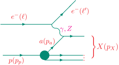
Figure 1: Deep inelastic electron-proton scattering: $q=\ell-\ell^{\prime},\;\nu=qp_{p}/m_{p},\;x\equiv x_{Bj}=-q^{2}/(2m_{p}\nu)$, $\ell(\ell^{\prime})$ is the four-momentum of the initial(final) $e^{-}$, $p_{A}$ is the four-momentum of $A,\;A=a,p$, where $a$ is a parton.

The limit of Bjorken is then of interest here, in which we take $Q^{2}\rightarrow\infty$ with $x$ fixed. In this limit, where here we will for reasons of pedagogy focus on the photon exchange in Fig. 1 , the standard methods can be used to represent the imaginary part of the attendant current-proton forward scattering amplitude as

$$\begin{split}W^{EM}_{\alpha\beta}(p_{p},q)&=\frac{1}{2\pi}\int d^{4}ye^{iqy}<p|[J^{EM}_{\beta}(y),J^{EM}_{\alpha}(0)]|p>\\ &=\qquad(-g_{\alpha\beta}+q_{\alpha}q_{\beta}/q^{2})W_{1}(\nu,q^{2})\\ &\qquad+\frac{1}{m_{p}^{2}}(p_{p}-qqp_{p}/q^{2})_{\alpha}(p_{p}-qqp_{p}/q^{2})_{\beta}W_{2}(\nu,q^{2})\end{split}$$ (1)

Here, $J^{EM}_{\alpha}(y)$ is the hadronic electromagnetic current and $W_{1,2}$ are the usual deep inelastic the structure functions, which first were shown to exhibit Bjorken scaling by the SLAC-MIT experiments [11] already at $Q^{2}\cong 1_{+}\text{GeV}^{2}$, precocious scaling – we return to this point below. For our purposes here, henceforward we drop the superscript on $J^{EM}$ so that $J^{EM}\equiv J$ for ease of notation and we always understand the average over the spin of the proton even when we do not indicate so explicitly. In Bjorken’s limit, we have

$$\begin{split}\lim_{Bj}m_{p}W_{1}(\nu,q^{2})&=F_{1}(x)\\ \lim_{Bj}\nu W_{2}(\nu,q^{2})&=F_{2}(x)\end{split}$$ (2)

where the scaling limits $F_{1,2}$ only depend on Bjorken’s variable $x$ and we denote

$$\lim_{Bj}\equiv\lim_{Q^{2}\rightarrow\infty}|_{x-\text{fixed}}.$$

The QCD theory of Gross, Wilczek and Politzer [2] provides a quantum field theoretic explanation of the observed Bjorken scaling behavior via Wilson’s OPE.

Specifically, in Bjorken’s limit, the phase in integral over space-time in (1) oscillates rapidly except in regions where it is bounded so that the value of the integral is dominated by the latter regions, which are well-known to correspond to the tip of the light-cone [13], the short-distance regime. Using Wilson’s expansion in this regime, we get the OPE [8, 9, 10]

$$\begin{split}J_{\beta}(y)J_{\alpha}(0)&=\frac{1}{2}g_{\beta\alpha}\left(\frac{\partial}{\partial y}\right)^{2}\frac{1}{y^{2}-i\epsilon y_{0}}{\sum_{n=0}^{\infty}}\sum_{j}C^{(n)}_{j,1}(y^{2}-i\epsilon y_{0})O^{j}_{\mu_{1}\cdots\mu_{n}}(0)y^{\mu_{1}}\cdots y^{\mu_{n}}\\ &+\frac{1}{y^{2}-i\epsilon y_{0}}{\sum_{n=0}^{\infty}}\sum_{j}C^{(n)}_{j,2}(y^{2}-i\epsilon y_{0})O^{j}_{\beta\alpha\mu_{1}\cdots\mu_{n}}(0)y^{\mu_{1}}\cdots y^{\mu_{n}}+\cdots,\end{split}$$ (3)

where we have neglected gradient terms without loss of content for our purposes here and as usual $\epsilon\downarrow 0$. We also note that $\{O^{j}_{\mu_{1}\cdots\mu_{n}}(y)\}$ are traceless, symmetric spin $n$ operators of dimension $n+2$ or of twist = dimension -spin = 2 [13]. The $\cdots$ represent operators of higher twist that are suppressed by powers of $q^{2}$ to any finite order in perturbation theory. The coefficient c-number functions $\{C^{(n)}_{j,k}\}$ are dimensionless and can be computed in renormalized perturbation theory.

Continuing our recapitulation of the methods in Refs. [8, 9, 10], if we define the spin averaged proton matrix elements of the operators $O^{j}$ via

$$<p|O^{j}_{\mu_{1}\cdots\mu_{n}}(0)|p>|_{\text{spin averaged}}=i^{n}\frac{1}{m_{p}}{p_{p}}_{\mu_{1}}\cdots{p_{p}}_{\mu_{n}}M^{n}_{j}+\cdots,$$ (4)

where the second $\cdots$ denotes trace-terms, we get the following relationship [8, 9, 10, 14] between the moments of the structure functions and the Fourier transforms of the coefficient functions:

$$\begin{split}\int_{0}^{1}dxx^{n}F_{1}(x,q^{2})&=\sum_{j}\bar{C}^{(n+1)}_{j,1}(q^{2})M^{n+1}_{j},\\ \int_{0}^{1}dxx^{n}F_{2}(x,q^{2})&=\sum_{j}\bar{C}^{(n)}_{j,2}(q^{2})M^{n+2}_{j},\end{split}$$ (5)

where [8]

$$\bar{C}^{(n)}_{j,k}(q^{2})=\frac{1}{2}i(q^{2})^{n+1}\left(-\frac{\partial}{\partial q^{2}}\right)^{n}\int d^{4}ye^{iqy}{\small\frac{C^{(n)}_{j,k}(y^{2})}{y^{2}-i\epsilon y_{0}}}.$$ (6)

The $q^{2}$ dependence of the $\bar{C}^{(n)}$ is controlled by the Callan-Symanzik equation [4] which reads

$$\left[\left(\mu\frac{\partial}{\partial\mu}+\beta(g)\frac{\partial}{\partial g}\right)\delta_{ij}-\gamma^{(n)}_{ij}(g)\right]C^{(n)}_{j,k}=0$$ (7)

where $\mu$ denotes the renormalization scale,

$$\beta(g)=\mu\frac{\partial g}{\partial\mu}$$

for the attendant renormalized coupling $g$, and the anomalous dimension matrix $\gamma^{(n)}_{ij}(g)$ is given as

$$\gamma^{(n)}_{ij}(g)=\left(Z_{O}^{-1}\mu\frac{\partial}{\partial\mu}Z_{O}\right)_{ij}|_{g_{0},\text{regularization fixed}}$$ (8)

where the operators $O^{(n)}_{j}\equiv O^{j}_{\mu_{1}\cdots\mu_{n}}$ are renormalized via

$$O^{(n)}_{i}\equiv O^{(n)}_{i,R}=\sum_{j}O^{(n)}_{j,bare}\left(Z_{O}^{-1}\right)_{ji}$$ (9)

so that they mix under renormalization in the well-known way [8, 9] and we use a standard notation of the renormalized, $R$, and unrenormalized , bare, operator representatives. $g_{0}$ is the bare coupling constant. It is well-known that the solution of (7) leads to the conclusion that the asymptotic Bjorken limit is controlled by the operators with the smallest eigenvalue for their anomalous dimension matrix in an asymptotically free theory such as the QCD [2] which we have in mind here. The implied behavior for the RHS of (5) is in agreement with experiment [11]. Here, we want to focus on the IR-improvement of the $C^{(n)}_{j,k},\;M^{n}_{j}$.

3 IR-Improved OPE

The isolation of the infrared aspects of the $C^{(n)}_{j,k}$ is immediate if we use the fundamental particles in the respective Lagrangian quantum field theory, quarks and gluons in the case of QCD, to evaluate the essential anomalous dimension matrix elements $\gamma^{(n)}_{ij}(g)$, as this is equivalent to studying deep inelastic scattering from these fundamental particles and takes us immediately, at least conceptually, to the parton model perspective studied famously by many [15, 16, 17, 18, 19, 20].

Specifically, we then focus on the parton level version of hadronic tensor $W_{\alpha\beta}$ which for definiteness we associate with a fermion $F$ in the underlying asymptotically free theory(QCD):

$$\begin{split}W^{F}_{\alpha\beta}(p_{F},q)&=\frac{1}{2\pi}\int d^{4}ye^{iqy}<p_{F}|[J_{\beta}(y),J_{\alpha}(0)]|p_{F}>\\ &=(2\pi)^{3}\sum_{X}\delta(q+p_{F}-p_{X})<p_{F}|J_{\beta}(0)|p_{X}><p_{X}|J_{\alpha}(0)|p_{F}>,\end{split}$$ (10)

where we use the fact that $q^{0}>0$ to drop the remaining term in the commutator and we always average over the spin of the fermion $F$, as we do for the proton$p$. We see clearly from (1) that the RHS of (10) and that of (1) involve the same OPE.

We first focus on the matrix element

$${\cal M}_{X,\alpha}\equiv<p_{X}|J_{\alpha}(0)|p_{F}>.$$ (11)

Following Refs. [5, 6], we isolate the dominant virtual IR divergences associated to the incoming line via the formula

$${\cal M}_{X,\alpha}=e^{\alpha_{s}\;B_{QCD}}<p_{X}|J_{\alpha}(0)|p_{F}>_{IRI-virt},$$ (12)

where the virtual infrared function $B_{QCD}$ is given in Refs. [5, 6]. The RHS of this last equation is valid to all orders in $\alpha_{s}\equiv g^{2}/(4\pi)$ so that one computes $<p_{X}|J_{\alpha}(0)|p_{F}>_{IRI-virt}$ from $<p_{X}|J_{\alpha}(0)|p_{F}>$ by comparing the coefficients of the powers of $\alpha_{s}$ on both sides of (12) iteratively.

Introducing this result into (10), we arrive at

$$\begin{split}W^{F}_{\alpha\beta}(p_{F},q)&=(2\pi)^{3}\sum_{X}\delta(q+p_{F}-p_{X})e^{2\alpha_{s}\Re B_{QCD}}\;\;{{}_{IRI-virt}\!<p_{F}|J_{\beta}(0)|p_{X}>}\\ &\qquad\qquad\;\;\;\;<p_{X}|J_{\alpha}(0)|p_{F}>_{IRI-virt}.\end{split}$$ (13)

We next isolate the leading soft, spin independent real emission infrared function associated to the incoming line as follows. We first separate $\{X\}$ into its multiple gluon subspaces via

$$\{X\}=\{X:X=X^{\prime}\otimes\{G_{1}\otimes\ldots\otimes G_{n}\},\text{for some}\;n\geq 0,X^{\prime}\;\text{is non-gluonic}\}.$$ (14)

Then we have

$$\begin{split}&e^{2\alpha_{s}\Re B_{QCD}}{{}_{IRI-virt}\!<p_{F}|J_{\beta}(0)|p_{X}>}<p_{X}|J_{\alpha}(0)|p_{F}>_{IRI-virt}\\ &=e^{2\alpha_{s}\Re B_{QCD}}\Big{[}\tilde{S}_{QCD}(k_{1})\cdots\tilde{S}_{QCD}(k_{n})\;\;{{}_{IRI-virt}<p_{F}|J_{\beta}(0)|p_{X^{\prime}}>}\\ &<p_{X^{\prime}}|J_{\alpha}(0)|p_{F}>_{IRI-virt}+\cdots+{{}_{IRI-virt\&real}\!<p_{F}|J_{\beta}(0)|p_{X^{\prime}},k_{1},\cdots,k_{n}>}\\ &<p_{X^{\prime}},k_{1},\cdots,k_{n}|J_{\alpha}(0)|p_{F}>_{IRI-virt\&real}\Big{]},\end{split}$$ (15)

where the real infrared function $\tilde{S}_{QCD}(k)$ is given in Refs. [5, 6]. The IR-improved quantities

$${{}_{IRI-virt\&real}\!<p_{F}|J_{\beta}(0)|p_{X}>}<p_{X}|J_{\alpha}(0)|p_{F}>_{IRI-virt\&real}$$

are defined iteratively from (12),(15) to all orders in $\alpha_{s}$ and they no longer contain the infrared singularities from the initial line associated to $B_{QCD}$ and to $\tilde{S}_{QCD}$, although, because of the non-Abelian infrared algebra of the theory, they do contain other IR singularities which of course cancel in the structure functions by the KNL theorem for massless fundamental fermions. For massive fundamental fermions, these latter singularities also cancel provided we resum the theory as we are doing here accordingly – see Refs. [21].

Introducing the representation in (15) into (10) we get

$$\begin{split}W^{F}_{\beta\alpha}(p_{F},q)&=(2\pi)^{3}\sum_{X}\delta(q+p_{F}-p_{X})e^{2\alpha_{s}\Re B_{QCD}}\Big{[}\tilde{S}_{QCD}(k_{1})\cdots\tilde{S}_{QCD}(k_{n})\\ &\qquad\qquad{{}_{IRI-virt}<p_{F}|J_{\beta}(0)|p_{X^{\prime}}>}<p_{X^{\prime}}|J_{\alpha}(0)|p_{F}>_{IRI-virt}+\cdots\\ &\qquad\qquad\;\;+{{}_{IRI-virt\&real}\!<p_{F}|J_{\beta}(0)|p_{X^{\prime}},k_{1},\cdots,k_{n}>}\\ &\qquad\qquad\;\;<p_{X^{\prime}},k_{1},\cdots,k_{n}|J_{\alpha}(0)|p_{F}>_{IRI-virt\&real}\Big{]}\\ &=\frac{1}{2\pi}\int d^{4}y\sum_{X^{\prime}}\sum_{n}\frac{1}{n!}\int\Pi_{j=1}^{n}\frac{d^{3}k_{j}}{k^{0}_{j}}e^{SUM_{IR}(QCD)}e^{iy(q+p_{F}-p_{X^{\prime}}-\sum_{j}k_{j})+D_{QCD}}\\ &\qquad\qquad\;\;{{}_{IRI-virt\&real}<p_{F}|J_{\beta}(0)|p_{X^{\prime}},k_{1},\cdots,k_{n}>}\\ &\qquad\qquad\;\;<p_{X^{\prime}},k_{1},\cdots,k_{n}|J_{\alpha}(0)|p_{F}>_{IRI-virt\&real}\\ &=\frac{1}{2\pi}\int d^{4}ye^{iqy}e^{SUM_{IR}(QCD)+D_{QCD}}\\ &\qquad\qquad\;\;{{}_{IRI-virt\&real}\!<p_{F}|}[J_{\beta}(y),J_{\alpha}(0)]|p_{F}>_{IRI-virt\&real},\end{split}$$ (16)

where we have defined

$${\rm SUM_{IR}(QCD)}=2\alpha_{s}\Re B_{QCD}+2\alpha_{s}\tilde{B}_{QCD}(K_{\rm max}),$$

$$2\alpha_{s}\tilde{B}_{QCD}(K_{\rm max})=\int{d^{3}k\over k^{0}}\tilde{S}_{\rm QCD}(k)\theta(K_{\rm max}-k),$$

$$D_{\rm QCD}=\int{d^{3}k\over k}\tilde{S}_{\rm QCD}(k)\left[e^{-iy\cdot k}-\theta(K_{\rm max}-k)\right],$$ (17)

and we stress that (16) does not depend on $K_{max}$. Using the standard partonic view, by which we have

$$W_{\beta\alpha}=\sum_{a}\int_{0}^{1}\frac{dx}{x}{\cal F}_{a}(x)W^{a}_{\beta\alpha}$$ (18)

for appropriately defined parton distribution functions $\{{\cal F}_{a}\}$, we introduce the OPE in (3) into (16) and use (1) to get the IR-improved results

$$\begin{split}\int_{0}^{1}dxx^{n}F_{1}(x,q^{2})&=\sum_{j}\tilde{\bar{C}}^{(n+1)}_{j,1}(q^{2})\tilde{M}^{n+1}_{j},\\ \int_{0}^{1}dxx^{n}F_{2}(x,q^{2})&=\sum_{j}\tilde{\bar{C}}^{(n)}_{j,2}(q^{2})\tilde{M}^{n+2}_{j},\end{split}$$ (19)

where [8]

$$\tilde{\bar{C}}^{(n)}_{j,k}(q^{2})=\frac{1}{2}i(q^{2})^{n+1}\left(-\frac{\partial}{\partial q^{2}}\right)^{n}\int d^{4}ye^{iqy}e^{SUM_{IR}(QCD)+D_{QCD}}{\small\frac{\tilde{C}^{(n)}_{j,k}(y^{2})}{y^{2}-i\epsilon y_{0}}}$$ (20)

and now

$$\begin{split}<p|\tilde{O}^{j}_{\mu_{1}\cdots\mu_{n}}(0)|p>|_{\text{spin averaged}}&\equiv\\ {}_{IRI-virt\&real}\!<p|O^{j}_{\mu_{1}\cdots\mu_{n}}(0)|p>_{IRI-virt\&real}|_{\text{spin averaged}}&=i^{n}\frac{1}{m_{p}}{p_{p}}_{\mu_{1}}\cdots{p_{p}}_{\mu_{n}}\tilde{M}^{n}_{j}\\ &\qquad+\cdots,\end{split}$$ (21)

where the second $\cdots$ again denotes trace-terms and the $\{\tilde{C}^{(n)}_{j,k}\}$ are the respective (new) IR-improved OPE coefficient functions. The $q^{2}$ dependence of the $\tilde{\bar{C}}^{(n)}$ is also controlled by the Callan-Symanzik equation [4] which now reads

$$\left[\left(\mu\frac{\partial}{\partial\mu}+\beta(g)\frac{\partial}{\partial g}\right)\delta_{ij}-\tilde{\gamma}^{(n)}_{ij}(g)\right]\tilde{\bar{C}}^{(n)}_{j,k}=0$$ (22)

where now the new matrix $\tilde{\gamma}^{(n)}_{ij}(g)$ is determined by the renormalization properties of the IR-improved matrix elements in (21) as we will discuss presently. We need to stress that in writing (20) we work to one-loop order in the various coefficients in this paper.

A convenient starting point for obtaining the new matrix $\tilde{\gamma}^{(n)}_{ij}(g)$ is presented by the pioneering analysis of the authors in Ref. [19, 20]. Working directly from the the representation in (18), the authors in Ref. [19] make contact with the matrix $\gamma^{(n)}_{ij}(g)$ for the unimproved OPE as follows. Focusing for definiteness for the moment on the non-singlet operator [8] ${}^{N}\!O^{F,b}(y)=\frac{1}{2}i^{N-1}S\bar{\psi}(y)\gamma_{\mu_{1}}\nabla_{\mu_{2}}\cdots\nabla_{\mu_{N}}\lambda^{b}\psi(y)-\text{trace terms}$, where $\nabla_{\mu}=\partial_{\mu}+ig\tau^{a}A^{a}_{\mu}$ is the covariant derivative, $\lambda^{b}$ is a flavor group generator and $S$ denotes symmetrization with respect to the indices $\mu_{1}\cdots\mu_{n}$, we have the matrix element between fundamental fermion states, where spin averaging is understood here as well, as

$$<p|^{N}\!O^{F,b}(y)|p>=\;^{F,b}\!O^{N}(\alpha_{s},\epsilon)p_{\mu_{1}}\cdots p_{\mu_{N}}-\text{trace terms}$$ (23)

where we use $d=4-\epsilon$ dimensions for regularization and the notation ${}^{F,b}\!O^{N}(\alpha_{s},\epsilon)\equiv M^{N}_{F,b}$ to make immediate contact with the arguments in Ref. [19]. The renormalized matrix element ${}^{F,b}\!O^{N}(\alpha_{s},\epsilon)$ is related to the bare one as we have indicated in (9):

$${}^{F,b}\!O^{N}(\alpha_{s},\epsilon,p^{2}/\mu^{2})=Z^{-1}_{O}(\alpha_{s},\frac{1}{\epsilon})\;^{F,b}\!O^{N}_{bare}((\alpha_{s})(\mu^{2}/p^{2})^{\epsilon},\epsilon)$$ (24)

so that collinear divergences are regularized by taking $p^{2}\neq 0$ in the approach in Ref. [19]. Using an arbitrary vector $\Delta$ with $\Delta^{2}=0$ we get

$${}^{F,b}\!O^{N}(\alpha_{s},\epsilon)=<p|^{N}\!O^{F,b}_{\mu_{1}\cdots\mu_{N}}(y)|p>\Delta^{\mu_{1}}\cdots\Delta^{\mu_{N}}/(\Delta p)^{N}.$$ (25)

The pole part of ${}^{F,b}\!O^{N}$ which is the renormalization part $Z^{-1}_{O}$ can be determined in any gauge by gauge invariance. We set $\Delta=n$ where $x_{Bj}=np/np_{p},\;x=kn/np$ and $nA^{a}=0$ so that we are in a light-like gauge. This allows us to write, following Ref. [19],

$${}^{F,b}\!O^{N}(\alpha_{s},\epsilon)=\int_{-1}^{1}dxx^{N-1}\;{{}^{F,b}\!O(x,\alpha_{s},\epsilon)}$$ (26)

where

$${{}^{F,b}\!O(x,\alpha_{s},\epsilon)}=Z_{F}[\delta(x-1)+x\frac{\int d^{d}k}{(2\pi)^{d}}\delta(x-\frac{kn}{pn})[\frac{\not\!n}{4kn}T(p,k)\not\!p]$$ (27)

where we use the notation of Ref. [19] so that $T(p,k)$ is the respective fully connected four-point function and $[\not\!bB$ denotes $\sum_{\alpha\alpha^{\prime}}b_{\alpha\alpha^{\prime}}B^{\alpha\alpha^{\prime}}_{\beta\beta^{\prime}}$ with corresponding notation for $B\not\!b]$. $Z_{F}$ is the fermion field renormalization constant as usual. By first analytically continuing the LHS of (24) to $d=4+\epsilon$ dimensions with $\epsilon>0$ the authors in Ref. [19] note that the limit $p^{2}\rightarrow 0$ gives the RHS as just $Z^{-1}_{O}(\alpha_{s},\epsilon)$ for an appropriate normalization of $\lambda^{b}$ . The RHS of (26) may then related to the moments of the densities of partons in a quark, $\Gamma_{S}(x,\alpha_{s},1/\epsilon)$ in the notation of Ref. [19], by writing a dispersion relation for $[(\not\!n/(4kn))T(p,k)\not\!p]$ and performing the attendant $k^{2}$ integral by closing the contour around the dispersive poles(see Sect. 4.2 of Ref. [19]), analytically continuing to $d=4+\epsilon$ dimensions with again $\epsilon>0$ and finally taking the limit $p^{2}\rightarrow 0$ to get

$$Z^{-1}_{O}(\alpha_{s},\frac{1}{\epsilon})=\int_{-1}^{1}dxx^{N-1}[\Gamma_{qq}(x,\alpha_{s},\frac{1}{\epsilon})\theta(x)-\Gamma_{q\bar{q}}(-x,\alpha_{s},\frac{1}{\epsilon})\theta(-x)]$$ (28)

where $\Gamma_{qq}(\Gamma_{q\bar{q}})$ is the respective parton density for a quark(anti-quark) in a quark. The coefficients of $\frac{1}{\epsilon}$ on both sides of this last equation then give the fundamental result, derived in Ref. [19],

$$\begin{split}-\gamma^{(N)}(\alpha_{s})&=2\int_{-1}^{1}dxx^{N-1}[P_{qq}(x,\alpha_{s})\theta(x)-P_{q\bar{q}}(-x,\alpha_{s})\theta(-x)]\\ &=2[P_{qq}(N,\alpha_{s})+(-1)^{N}P_{q\bar{q}}(N,\alpha_{s})]\end{split}$$ (29)

where we define

$$F(N)=\int_{0}^{1}dxx^{N-1}F(x)$$

and the $P_{BA}$ are the usual DGLAP-CS [3, 4] splitting kernels defined in the convention of Ref. [19] and $\gamma^{(N)}(\alpha_{s})$ is the respective anomalous dimension of the operator ${}^{N}\!O^{F,b}$.

To apply this calculation to our new anomalous dimension matrix we IR-improve it at each step as we have shown above (and as we have shown for the IR-improved DGLAP-CS theory in Refs. [5, 6]), so that we replace

$$<p|^{N}\!O^{F,b}(y)|p>\rightarrow<p|^{N}\!\tilde{O}^{F,b}(y)|p>$$

as defined in (21) with the corresponding substitution of ${}^{F,b}\!O^{N}(\alpha_{s},\epsilon)$ by the analogous ${}^{F,b}\!\tilde{O}^{N}(\alpha_{s},\epsilon)$. This leads to the relationship

$${}^{F,b}\!\tilde{O}^{N}(\alpha_{s},\epsilon,p^{2}/\mu^{2})=Z^{-1}_{\tilde{O}}(\alpha_{s},\frac{1}{\epsilon})\;^{F,b}\!\tilde{O}^{N}_{bare}((\alpha_{s})(\mu^{2}/p^{2})^{\epsilon},\epsilon)$$ (30)

between the renormalized and bare IR-improved matrix elements. The analoga of (26) and (27) are then

$${}^{F,b}\!\tilde{O}^{N}(\alpha_{s},\epsilon)=\int_{-1}^{1}dxx^{N-1}\;{{}^{F,b}\!\tilde{O}(x,\alpha_{s},\epsilon)}$$ (31)

where

$${{}^{F,b}\!\tilde{O}(x,\alpha_{s},\epsilon)}=Z_{F}[\delta(x-1)+x\frac{\int d^{d}k}{(2\pi)^{d}}\delta(x-\frac{kn}{pn})[\frac{\not\!n}{4kn}\tilde{T}(p,k)\not\!p]$$ (32)

and we continue to use the notation of Ref. [19] so that $\tilde{T}(p,k)$ is the respective IR-improved fully connected four-point function obtained from the unimproved one, $T(p,k)$, by using the master formula Eq.(1) in Refs. [6] restricted to its QCD aspect, for example. This means that we get the analog of (28) as

$$Z^{-1}_{\tilde{O}}(\alpha_{s},\frac{1}{\epsilon})=\int_{-1}^{1}dxx^{N-1}[\Gamma^{exp}_{qq}(x,\alpha_{s},\frac{1}{\epsilon})\theta(x)-\Gamma^{exp}_{q\bar{q}}(-x,\alpha_{s},\frac{1}{\epsilon})\theta(-x)]$$ (33)

where $\Gamma^{exp}_{qq},\;\Gamma^{exp}_{q\bar{q}}$ are the respective IR-improved parton densities. We get in this way the identification of the respective IR-improved anomalous dimension as

$$-\tilde{\gamma}^{(N)}(\alpha_{s})=2\frac{\alpha_{s}}{2\pi}[P^{exp}_{qq}(N,\alpha_{s})+(-1)^{N}P^{exp}_{q\bar{q}}(N,\alpha_{s})]$$ (34)

where the $P^{exp}_{qq},\;P^{exp}_{q\bar{q}}$ are the respective IR-improved kernels as introduced in Refs. [5, 6], where we advise that the notation of Ref. [19] differs from that in Refs. [5, 6] by whether or not one includes the factor $\alpha_{s}/(2\pi)$ on the RHS of (30) in the definition of the kernels. This allows us to write at IR-improved one-loop level the identifications

$$-\tilde{\gamma}^{(N)}(\alpha_{s})_{ij}=2\frac{\alpha_{s}}{2\pi}P^{exp}_{ij}(N)$$ (35)

where the labels $i,j$ span the usual values for the one-loop anomalous dimension matrix for the evolution of the parton distributions as given in Refs. [3, 4, 8, 9, 10] for example. This establishes in a rigorous way the connection between the IR-improved DGLAP-CS theory in Ref. [5, 6] and the OPE methods of Wilson as used by Refs. [8, 9, 10] in the study of deep inelastic lepton-nucleon scattering.

Evidently, this connection may be manifested in the analysis of other physical processes as well. We refer the reader to Refs. [6, 7] wherein the new precision-baseline MC Herwiri1.031 which realizes the IR-improved DGLAP-CS kernels has been introduced and compared to the Tevatron data [22, 23] on single Z production. Its application to the various physical processes at LHC is in progress and will appear accordingly elsewhere [24], where we need to stress that Herwiri1.031 can be applied to any process to which Herwig6.5 [25] can be applied and that it interfaces to MC@NLO [26] the same way that does Herwig6.5. As we have shown in Refs. [6, 7], we have an improved agreement between the IR-improved MC’s shower and the Tevatron data with no need of an abnormally large intrinsic transverse momentum parameter, PTRMS$\sim 2$GeV in the notation of Herwig [25], as it is required for similar agreement with Herwig6.5 [27]. We point-out that, consistent with the precociousness of Bjorken scaling, the IR-improved MC Herwiri.031 gives us a paradigm for reaching a precision QCD MC description of the LHC data, on an event-by-event basis with realistic hadronization from the Herwig6.5 environment, that does not involve an ad hoc hard scale parameter, where we define “hard” relative to the observed precociousness of Bjorken scaling. What we have shown in the discussion above is that this paradigm has a rigorous basis in quantum field theory. In closing, we thank Prof. Ignatios Antoniadis for the support and kind hospitality of the CERN TH Unit while part of this work was completed.

References

• [1] K. Wilson, Phys. Rev. 179 (1969) 1499; W. Zimmermann, in Lectures on Elementary Particles and Quantum Field Theory – 1970 Brandeis Summer Institute in Theoretical Physics, vol. 1, eds. S. Deser, H. Pendleton and M. Grisaru, (MIT Press, Cambridge, 1970) p. 395; R.A. Brandt and G. Preparata, Nucl. Phys. 27 (1971) 541.
• [2] D. J. Gross and F. Wilczek, Phys. Rev. Lett. 30 (1973) 1343; H. David Politzer, ibid.30 (1973) 1346; see also , for example, F. Wilczek, in Proc. 16th International Symposium on Lepton and Photon Interactions, Ithaca, 1993, eds. P. Drell and D.L. Rubin (AIP, NY, 1994) p. 593, and references therein.
• [3] G. Altarelli and G. Parisi, Nucl. Phys. B126 (1977) 298; Yu. L. Dokshitzer, Sov. Phys. JETP 46 (1977) 641; L. N. Lipatov, Yad. Fiz. 20 (1974) 181; V. Gribov and L. Lipatov, Sov. J. Nucl. Phys. 15 (1972) 675, 938; see also J.C. Collins and J. Qiu, Phys. Rev. D39 (1989) 1398.
• [4] C.G. Callan, Jr., Phys. Rev. D2 (1970) 1541; K. Symanzik, Commun. Math. Phys. 18 (1970) 227, and in Springer Tracts in Modern Physics, 57, ed. G. Hoehler (Springer, Berlin, 1971) p. 222; see also S. Weinberg, Phys. Rev. D8 (1973) 3497.
• [5] B.F.L. Ward, Adv. High Energy Phys. 2008 (2008) 682312.
• [6] B.F.L. Ward, Ann. Phys. 323 (2008) 2147; B.F.L. Ward, S.K. Majhi and S.A. Yost, arXiv:1201.0515, in PoS(RADCOR2011), in press.
• [7] S. Joseph, S. Majhi, B.F.L. Ward and S.A. Yost, Phys. Lett. B685 (2010) 283; Phys. Rev. D81 (2010) 076008.
• [8] D.J. Gross and F. Wilczek, Phys. Rev.D8 (1973) 3633; ibid. 8 (1974) 980.
• [9] H. Georgi and H.D. Politzer, Phys. Rev. D9 (1974) 416, and references therein.
• [10] H.D. Politzer, Phys. Rept. 14 (1974) 129.
• [11] See for example R.E. Taylor, Phil. Trans. Roc. Soc. Lond. A359 (2001) 225, and references therein.
• [12] J. Bjorken, in Proc. 3rd International Symposium on the History of Particle Physics: The Rise of the Standard Model, Stanford, CA, 1992, eds. L. Hoddeson et al. (Cambridge Univ. Press, Cambridge, 1997) p. 589, and references therein.
• [13] D.J. Gross and S.B. Treiman, Phys. Rev. D4 (1971) 2105; ibid. 4 (1971) 1059, and references therein.
• [14] N. Christ, B. Hasslacher and A.H. Mueller, Phys. Rev. D6 (1972) 3543.
• [15] R.P. Feynman, Phys. Rev. Lett. 23 (1969) 1415; Photon-Hadron Interactions, (Benjamin, New York, 1972).
• [16] J.D. Bjorken and E.A. Paschos, Phys. Rev. 185 (1969) 1975; Phys.Rev. D1 (1970) 3151, and references therein.
• [17] S.D. Drell and T.-M. Yan, Phys. Rev. Lett. 25 (1970) 316; ibid.25 (1970) 902; S.D. Drell, D.J. Levy and T.-M. Tan, Phys. Rev. D1 (1970) 1617; ibid.1 (1970) 1035; Phys.Rev. 187 (1969) 2159, and references therein.
• [18] R.K. Ellis et al., Phys. Lett. B 78 (1978) 281.
• [19] C. Curci, W. Furmanski and R. Petronzio, Nucl.Phys. B175 (1980) 27.
• [20] W. Furmanski and R. Petronzio, Phys.Lett. B 97 (1980) 437.
• [21] B.F.L. Ward, Phys.Rev. D78 (2008) 056001; C. Di’Lieto, S. Gendron, I.G. Halliday, and C.T. Sachradja, Nucl. Phys.B183(1981) 223; R. Doria, J. Frenkel and J.C. Taylor, ibid. 168 (1980) 93; S. Catani, M. Ciafaloni and G. Marchesini, Nucl. Phys.B264 (1986) 588; S. Catani, Z. Phys. C37 (1988) 357, and references therein.
• [22] V.M. Abasov et al., Phys. Rev. Lett. 100 (2008) 102002.
• [23] C. Galea, in Proc. DIS 2008, London, 2008, http://dx.doi.org/10.3360/dis.2008.55.
• [24] B.F.L. Ward, to appear.
• [25] G. Corcella et al., hep-ph/0210213; J. High Energy Phys. 0101 (2001) 010; G. Marchesini et al., Comput. Phys. Commun.67 (1992) 465.
• [26] S. Frixione and B.Webber, J. High Energy Phys. 0206 (2002) 029; S. Frixione et al., arXiv:1010.0568.
• [27] M. Seymour, private communication.