Gas Excitation in ULIRGs:
Maps of Diagnostic Emission-Line Ratios in Space and Velocity

Abstract

Emission-line spectra extracted at multiple locations across 39 ultraluminous infrared galaxies have been compiled into a spectrophotometric atlas. Line profiles of H$\alpha$, [N II], [S II], [O I], H$\beta$, and [O III] are resolved and fit jointly with common velocity components. Diagnostic ratios of these line fluxes are presented in a series of plots, showing how the Doppler shift, line width, gas excitation, and surface brightness change with velocity at fixed position and also with distance from the nucleus. One general characteristic of these spectra is the presence of shocked gas extending many kiloparsecs from the nucleus. In some systems, the shocked gas appears as part of a galactic gas disk based on its rotation curve. These gas disks appear primarily during the early stages of the merger. The general characteristics of the integrated spectra are also presented.

1. Introduction

The optical emission-line spectrum of a galaxy is a powerful diagnostic of recent star formation (Kennicutt, 1998), the gas-phase metallicity (Kewley et al., 2006), and the excitation mechanism (Kewley et al., 2001; Baldwin et al., 1981). Fiber spectra of low redshift galaxies have provided the first systematic examination of these properties in the central regions of low redshift galaxies (e.g. Kauffmann et al., 2003a, b; Tremonti et al., 2004). Infrared spectra obtained with the new generation of multi-object spectrographs, including the James Webb Space Telescope, will make it possible to apply these diagnostics over the entire period of galaxy evolution. The interpretation of these spectra, however, is complicated by measurement apertures that subtend a kiloparsec or more.

On scales larger than the narrow line region of an active galactic nucleus (AGN) or a giant HII region, the physical process that excites the gas is not necessarily uniform. The contribution to the excitation from shocks or the hard spectrum of an AGN must be properly identified in order to use metallicity and star formation diagnostics constructed under the assumption of photoionization by massive stars.

To address this problem, we obtain spectra that resolve scales of $\sim$1 kpc and map the excitation across a sample of ultraluminous infrared galaxies (ULIRGs). Ratios of forbidden lines to Balmer lines are interpreted using grids of photoionization models and “BPT diagrams” (Baldwin et al., 1981). Flux ratios of lines that are close in wavelength, i.e. [N II]/H$\alpha$, [S II]/H$\alpha$, [O I]/H$\alpha$ and [O III]/H$\beta$, are used because they are insensitive to reddening. While the line ratios produced by a power-law spectral energy distribution are largely degenerate with those predicted by shock models (Allen et al., 2008), spatial mapping has proven effective at distguishing shock excitation from photoionization. The large extranuclear extent of strong forbidden-line emission relative to the Balmer lines (Colina et al., 2005; Monreal-Ibero et al., 2010; Rich et al., 2011) has uniquely identified shocks as the excitation mechanism in some ULIRGs. High forbidden-to-Balmer line ratios also appear to be common in the extranuclear regions of $z\sim 2$ galaxies mapped with infrared IFUs (Genzel et al., 2011; Law et al., 2007; Wright et al., 2010).

Previous studies have shown that broad line profiles are often associated with shock excitation in mergers (Rich et al., 2011). We improve upon these studies by resolving line profiles, using multiple component fitting, and examining emission line ratios in velocity space. Since the next generation of optical IFUs such as MUSE (Multi Unit Spectroscopic Explorer; Henault et al., 2003) and KCWI (Keck Cosmic Web Imager; Martin et al., 2010), will be able to map galaxies in the optical with large fields of view, our approach demonstrates how to analyze these data. We argue that measuring variations in the forbidden-to-Balmer line flux ratio in the velocity coordinate may prove as useful as resolution in the spatial dimension for determining the excitation mechanism.

The main parts of this paper are two sets of figures. The first set illustrates the variation of the forbidden-to-Balmer line flux ratio on scales of approximately 60 km s^-1 spectrally and 1-2 kpc spatially; it also compares the lines ratios to grids of photoionization models and shock models. The second set displays the emission-line profiles across 39 galaxies, selected from the IRAS 2 Jy survey (Murphy et al., 1996; Strauss et al., 1992, 1990) and known to be undergoing a galaxy merger. Section 2 presents the observations and explains the measurement procedure. The discussion is mostly qualitative, focusing on the trends observed during the progression of the merger. A companion paper (Soto et al. 2012b) provides a quantitative analysis of the relationship between the gas excitation and gas kinematics. Throughout the paper we use a cosmology with $\Omega_{m}=0.27$, $\Omega_{m}=0.73$, and $H_{0}=71$ km s^-1 Mpc^-1.

2. Data

2.1. Sample and Aperture Selection

Moderate-resolution spectra were obtained at Keck Observatory with the Echellete Spectrograph and Imager (ESI; Sheinis et al., 2002) under average seeing of 0$\farcs$8. The observations and data reduction are described in Martin (2005, 2006), where the Na I 5890, 96 interstellar absorption kinematics were measured previously and discussed for the 18 objects with published CO velocities. In the remaining 21 objects in the sample, redshifts were determined from the integrated H$\alpha$ emission line.

The broad spectral bandpass covers recombination lines from H and He and the following strong forbidden lines: [S II]$\lambda\lambda 6717,31$, [N II] $\lambda 6548,6584$, [O I] $\lambda 6300,64$, [O III]$\lambda 5007$, and sometimes [O II]$\lambda 3727,29$ at lower S/N ratio. Dust-insensitive line ratios constructed from a subset of these line flux measurements are presented in this paper for the full sample of 39 galaxies.

Table 1 lists the name, merger stage, infrared luminosity, and redshift of each galaxy. The galaxies have IR luminosities L${}_{IR}>8.5\times 10^{11}$ L_⊙, which identify them as ultraluminous infrared galaxies (ULIRGs) and and 60$\mu$m flux $>$ 1.94 Jy (Murphy et al., 1996). The redshift range from 0.043 to 0.15 corresponds to angular scales from 1.00 to 2.61 kpc/″. The position angle of the 20″ long slit is also listed for each galaxy.

Table 1 Sample and Morphology

IRAS Name	Merger Class	log($\frac{L_{IR}}{L_{\odot}}$)	$z$	PA
(1)	(2)	(3)	(4)	(5)
00153$+$5454	IIIb	12.10	0.1116	-22.0
00188$-$0856	V	12.33	0.1285	-3.3
00262$+$4251	IVa	12.08	0.0972	-14.1
01003$-$2238	V	12.25	0.1177	10.0
01298$-$0744	IVb	12.29	0.1362	-89.3
03158$+$4227	IVa	12.55	0.1344	-15.0
03521$+$0028	IIIb	12.48	0.1519	76.5
05246$+$0103	IIIa	12.05	0.0971	109.5
08030$+$5243	IVb	11.97	0.0835	0.0
08311$-$2459	IVb	12.40	0.1006	67.5
09111$-$1007	IVa	11.98	0.0542	73.5
09583$+$4714	IIIa	11.98	0.0859	124.0
10378$+$1109	IVb	12.23	0.1362	11.3
10494$+$4424	IVb	12.15	0.0923	25.0
10565$+$2448	M	11.98	0.0431	109.0
11095$-$0238	IVb	12.20	0.1065	10.0
11506$+$1331	V	12.27	0.1273	80.3
11598$-$0112	IVb	12.40	0.1507	130.0
12071$-$0444	IVb	12.31	0.1284	0.0
13451$+$1232	IIIb	12.27	0.1212	105.7
15130$-$1958	IVb	12.03	0.1094	116.0
15245$+$1019	IIIb	11.96	0.0755	127.8
15462$-$0405	IVb	12.16	0.1003	164.6
16090$-$0139	IVa	12.48	0.1336	107.6
16474$+$3430	IIIb	12.12	0.1115	161.8
16487$+$5447	IIIb	12.12	0.1038	66.2
17028$+$5817	IIIa	12.11	0.1061	94.5
17208$-$0014	IIIb	12.38	0.0428	166.7
17574$+$0629	IIIb	12.10	0.1096	51.2
18368$+$3549	IVa	12.19	0.1162	-31.0
18443$+$7433	V	12.23	0.1347	29.6
18470$+$3233	IIIa	12.02	0.0785	67.3
19297$-$0406	IVb	12.36	0.0857	149.5
19458$+$0944	IVa	12.31	0.1000	118.1
20046$-$0623	IIIb	12.02	0.0843	72.0
20087$-$0308	IIIb	12.39	0.1057	85.5
20414$-$1651	IVb	12.19	0.0869	12.6
23327$+$2913	IIIa	12.03	0.1075	-4.3
23365$+$3604	IIIb	12.13	0.0645	-19.5

Note. — Column 1: Name, Column 2: Merger Classification (Veilleux et al., 2002). Column 3: IR luminosity (Murphy et al., 1996). Column 4: Redshift. Column 6: Position angle of slit in degrees.

Fig.1 shows two examples from the full figure set in Appendix A. The left panel shows an $r$ band image of each ULIRG from Murphy et al. (1996). The slit position and the apertures used to extract spectra are marked. In the middle panel, the same apertures are marked and numbered on a cut-out of the two-dimensional spectrum near H$\alpha$ and [N II]. All spectral orders were spatially registered with the order containing H$\alpha$ by cross correlation of the spatial continuum profile. The location of the brightest continuum emission defines the position of Aperture 0; and the apertures are slightly separated ($\sim$ 0.1″) to reduce correlations between adjacent spectra. Measurements of the Doppler shift, velocity dispersion, and excitation are summarized in the rightmost panel and described in Sect.2.2.

In both galaxies included in Fig. 1, line emission is detected over a much larger angle than is the continuum emission. In the first example, the H$\alpha$ line profile of the low surface-brightness emission seen against the dark sky is noticeably smoother than the double-peaked profiles of the extraplanar gas emanating from nearby starbursts (Heckman et al., 1990; Lehnert & Heckman, 1996; Martin, 1998). The second example illustrates one of the 11 pre-mergers in the sample. Strong continuum emission is detected from two separate galaxies as well as an extended, tidal feature.

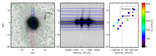
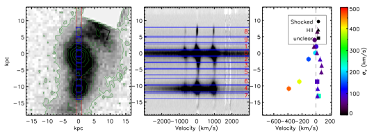
Figure 1.— Upper Row: IRAS11095-0238 - a single nucleus ULIRG. Lower Row: IRAS05246+0103 - a double nucleus ULIRG. Left Column: An $r$ band image from the Palomar 60 inch telescope (Murphy et al., 1996). The green contours represent the median, and the 1, 2, 3, 4, and 5 $\sigma$ surface brightness levels in the image. The red lines show the spatial position of the 1″$\times$20″ slit. The blue rectangles identify the positions of the selected apertures. Middle Column: The 2D spectrum of H$\alpha$ + [N II] centered in velocity space on H$\alpha$. The blue rectangles identify the pixels that contribute to the individual apertures. The redshift range of the sample allows each object to be sampled by several apertures along the slit. In IRAS 11095-0238 there is extended H$\alpha$ and [N II] emission, allowing measurement of excitation mechanism out to 11 kpc from the nucleus. Right Column: The position-velocity diagram for all of the fit components. The line width of the components is indicated by the color of the plot point. The plot symbol represents the excitation category for that individual spectral component.

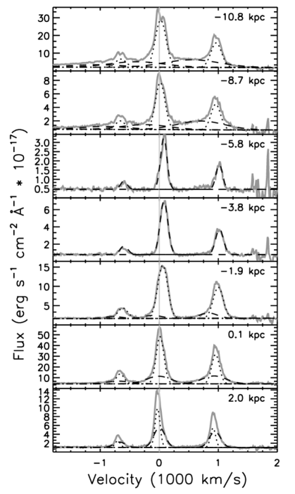
Figure 2.— For the transitions H$\alpha$ + [N II], we show the line profile for all positions in IRAS11095-0238 (above) and IRAS05246+0103 (below). Above: For IRAS11095-0238, the line profile shows a clear variation from aperture to aperture. In the aperture -2.7 kpc from the $r$ band nucleus, the broad component (dashed) is blue-shifted relative to the narrow (dotted) component. On the other side of the nucleus at 2.1 kpc from the center, the broad component is slightly red-shifted relative to the narrow component. Below: In IRAS05246+0103 there is more than one nucleus (positions: 0.1 kpc and -10.8 kpc). A broad component can be seen in the line profile in each of them.

2.2. Emission Line Fitting

In Appendix B, we show the observed emission line profiles as a function of aperture and of line transition for the full galaxy sample. In this section, we describe example figures for the same two galaxies as in Fig. 1. First, Fig. 2 shows the H$\alpha$+[N II] line profiles as a function of aperture position along the slit shown in Fig. 1. Prominent spatial gradients in the ratio of [N II] to H$\alpha$ flux can be easily seen by scanning up and down the first column for each galaxy. Fig. 2 illustrates the variation in the relative [N II] to H$\alpha$ strength along the slits shown in Fig. 1. The ratio is very high in the extended, low-surface brightness emission surrounding IRAS11095-0238. IRAS05246+0103 shows similar variation at the various positions coinciding with the few kpc regions around the nuclei. The variations in the velocity coordinate are more subtle but can be seen by comparing an unblended forbidden line, i.e., [O I] $\lambda$6300 or [O III] $\lambda$5007, with the H$\beta$ profile from the same aperture.

Next, in Fig. 3 we show the line profiles for a single aperture as a function of line transition. In the IRAS11095-0238 spectrum, the broad, blue wing on the [O I] $\lambda$6300 profile is clearly stronger (relative to the total line flux) than the wing on the H$\beta$ profile. IRAS05246+0103 shows this broad feature as well at in the measured transitions with H$\beta$ being weaker. We note that in the spectral direction, quantifying these variations in the diagnostic line ratios is challenging. The line profiles must be moderately well resolved, e.g., FWHM of 60 km s^-1 for these echellete spectra. Because the H$\alpha$, [N II], and [S II] lines are often broad enough to blend with neighboring lines, coverage of one or more unblended lines like [O I]  $\lambda$6300 is essential.

Our line fitting procedure consists of fitting multiple Gaussian components simultaneously to 8 transitions (H$\alpha$, [N II] $\lambda 6548,6583$, [S II]$\lambda\lambda 6717,31$, [O I] $\lambda 6300$, H$\beta$, and [O III]$\lambda 5007$) with MPFIT in IDL. The fitting method ties the individual kinematic components of the emission line profiles together, by requiring the same Doppler shift and velocity linewidth for all transitions. The amplitude of each component can vary independently. These requirements assume that the gas clouds that are identified by each kinematic component emit in all transitions. This method handles differing degrees of line blending by finding a solution suitable for all transitions. For some apertures, H$\beta$ absorption contributed by the underlying stellar population significantly affects the line profile. We therefore include an H$\beta$ absorption component in the fitting as well, but allow it to vary independently from those of the emission components (Soto & Martin, 2010).

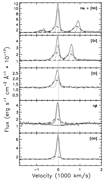
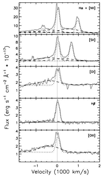
Figure 3.— For a single aperture in IRAS11095-0238 (Above) and IRAS05246+0103 (Below), we present the line profiles for all analyzed transitions. Two components are required to fit the asymmetric line profiles evident in each transition. The two components used in the fits have the same kinematics for each transition.

We determined the number of components to fit by comparing fitting residuals to the flux measurement errors. The fitting for each aperture starts with a single component fit to all of the lines. If the residual flux exceeds the measurement error over a resolution element (FWHM $>$ 70)  km s^-1, we include another fit component. We maintain spatial continuity in the fits by using the results from adjacent apertures as the initial guess for subsequent apertures.

Two fitting components typically characterized the line profiles of all measured transitions well, but we often see variations in amplitude and linewidth as a function of aperture and fitting component. The fit of these multiple components allows us to identify separate kinematic components that vary in spatially different ways (Fig. 2). The position-velocity diagrams in the right column of Fig. 1 (and in Appendix A) further illustrate these variations in the cases of IRAS11095-0238 and IRAS05246+0103. All of this suggests that multiple kinematic components at a fixed position often arise from physically distinct components of the galaxy and can be separated by this spatial and spectral deconstruction of the emission line profiles. We include a full description of the fitted kinematic components in Appendix C, Table LABEL:tab:flux.

2.3. Integrated Apertures

To allow examination of the impact of this spatial and kinematic structure seen in the spectral line ratios on the integrated spectrum, we extracted pseudo-integrated spectra. Using a large aperture that encompass all the apertures, the flux per pixel is summed over this aperture. The resulting integrated line profiles were fit using the technique described in Section 2.2. In Soto et al. (2012b) we compare the spectral components identified in these integrated spectra to the components in sub-apertures. Our analysis of the integrated spectra demonstrates when separate physical components, established on the basis of the spatially resolved spectra, can be recognized in velocity space in the integrated spectrum.

We use the integrated line fluxes for the individual galaxies in the mergers and classify their overall excitation type using line ratio comparisons (Kewley et al., 2006). Table 2.3 shows the result of these classifications. The HII class comprises the largest fraction of the sample (43%) in the shows the classification of these integrated spectra, while LINER and Seyfert classes make up 18% and 12% of the sample. Galaxies with mixed classifications in the different diagnostic diagram make up the remaining 27 % of the sample.

Table 2Integrated Spectral Classification

IRAS Name	$\rm\left(\frac{[N~{}II]/{\rm H}\alpha}{[O~{}III]/{\rm H}\beta}\right)$	$\rm\left(\frac{[S~{}II]/{\rm H}\alpha}{[O~{}III]/{\rm H}\beta}\right)$	$\rm\left(\frac{[O~{}I]/{\rm H}\alpha}{[O~{}III]/{\rm H}\beta}\right)$	Total
(1)	(2)	(3)	(4)	(5)
00153+5454	C	H/S	L/S	M
00153+5454	C	L	L	L
00188$-$0856	A	T	S	S
00262+4251	A	L	T	L
01003$-$2238	A	S	S	S
01298$-$0744	C	T	L	L
03158+4227	A	T	L	L
03521+0028	X	X	X	X
05246+0103	C/A	H	T	H
05246+0103	A	L	T	L
08030+5243	C	H	H	H
08311$-$2459	X	X	X	X
09111$-$1007	C	H	H	H
09583+4714	A	S	S	S
09583+4714	H	H	H	H
10378+1109	A	T	L	L
10494+4424	C/A	H	S/L	M
10565+2448	C	H	H	H
11095$-$0238	C	L	L	L
11506+1331	C	H	H/S	H
11506+1331	H	H	H/S	H
11598$-$0112	C	H	H	H
12071$-$0444	A	T	S	S
13451+1232	A	S	S	S
15130$-$1958	A	S	S	S
15245+1019	C	H	H	H
15245+1019	A	H	S/L	M
15462$-$0405	C	H	T	H
16090$-$0139	C/A	T	L	L
16474+3430	C	H	H	H
16474+3430	H	H	H	H
16487+5447	C	H	S/L	M
16487+5447	A	S/L	S/L	M
17028+5817	H	H	H	H
17028+5817	C	S/L	S/L	S/L
17208$-$0014	C	H	H	H
17574+0629	H	H	H	H
18368+3549	A	S/L	S/L	S/L
18443+7433	A	T	L	L
18470+3233	C	H	H	H
18470+3233	C	H	L	H/L
18470+3233	H	H	H	H
19297$-$0406	C	H	H	H
19458+0944	C	H	L	H/L
20046$-$0623	C	H	H	H
20087$-$0308	A	S/L	S/L	S/L
20414$-$1651	C	H	H/S	H
23327+2913	A	S/L	S/L	S/L
23365+3604	C	H	H

Note. — Column 1: IRAS Name. Column 2: Spectral classifications as defined in Kewley et al. (2006) with fluxes from the sum of both kinematic components in the spatially integrated measurements along the ESI longslit. These diagnostics come from the comparision of [N II]/H$\alpha$ vs. [O III]/H$\beta$. A refers to galaxies that exceed the maximum excitation possible from star formation alone suggesting a possible AGN, H refers to the regions below the empirical limit to the excitation by HII regions (Kauffmann et al., 2003a), C refers to the region between these, where the integrated emission line ratio is expected to be a combination of HII and AGN contributions. Column 3: Spectral classifications as defined in Kewley et al. (2006) for the line ratios [S II]/H$\alpha$ vs. [O III]/H$\beta$. L refers to line ratios indicating LINER, S refers to line ratios indicating a Seyfert galaxy. Column 4: Spectral classifications as defined in Kewley et al. (2006) for the line ratios [O I]/H$\alpha$ vs. [O III]/H$\beta$. Column 5: The total classification determined by combination of the 3 diagnostic diagrams. The additional classification of M is included where a mix of all three classifications makes the class designation ambiguous.

3. Results

3.1. Line Ratios

Deblending the line profiles allows us to investigate the underlying excitation mechanism that is relevant for each kinematic component. In the standard BPT diagram, ratios of forbidden transitions to Balmer transitions ([N II]/H$\alpha$, [S II]/H$\alpha$, [O I]/H$\alpha$ and [O III]/H$\beta$) probe the energy of the associated ionizing radiation (Baldwin et al., 1981). High forbidden to Balmer line ratios exceeding the range possible for star formation can imply the presence of either AGN (Kewley et al., 2006) or shocks (Allen et al., 2008).

In the right column of Fig. 1 (and in Appendix B), we present the kinematic components along with an indicator for the type of excitation that is most likely relevant. The top right panel of Fig. 1 is an example of one of the more irregular kinematic patterns for the galaxy IRAS11095-0238. In this case the entire galaxy has shock-like excitation. The lower right panel of Fig. 1 shows a different kinematic pattern the narrow HII-like emission in IRAS05246+0103 and broad shock-like emission closer to the nuclei.

3.2. Shock Models

Shock models predict the line ratios created by the shocks for a range of magnetic field strengths, densities, and shock velocities ($v_{sh}$; Allen et al., 2008). Here, we focus on magnetic field ranging from 1 to 100 $\mu$G for starburst galaxies (Thompson et al., 2006). The shock-only model with solar metallicity and electron density $n_{e}=10~{}{\rm cm}^{-3}$, overlapped with a large fraction of the measured line ratios. The line ratios fall into the region of the BPT diagram that more often suggests LINER-like excitation. If these measured line ratios can be attributed to shocks, the models suggests that the precursor to the shock is not a significant contributor to the ionization (Dopita & Sutherland, 1995). Some of the measured line ratios fall just below the shock grid, but the effect of averaging over an $\sim 1{\rm kpc}^{2}$ can include contributions by HII regions as well, moving the line ratio toward the HII region of the diagram. The spread in the [O I]/H$\alpha$ ratio with $v_{sh}$ in these models (Fig. 4) indicates that the [O I]/H$\alpha$ vs [O III]/H$\beta$ diagram is a more sensitive identifier of shocks and shock velocity. The [S II]/H$\alpha$ and [N II]/H$\alpha$ gridlines, on the other hand, pile-up for gridlines with $v_{sh}>250$  km s^-1.

In a different class of objects, line emitting red galaxies, extended LINER-like emission is detected at extended radii as well, but post-AGB stars are the suspected source of ionization (Yan & Blanton, 2012). These post-AGB stars would make the largest relative contribution to the ULIRG spectra at large galactocentric radii because there is an increase in stellar age with radius (Soto & Martin, 2010); the central regions are dominated by ongoing star formation. However, the ages of the stellar populations necessary to create this excitation are few Gyr, much larger than the $\sim 0.4$ Gyr implied by the measured stellar population ages. Furthermore, the scaling between H$\alpha$ luminosity and stellar mass from this form of excitation (Yan & Blanton, 2012) implies an order of magnitude more stellar mass ($2~{}\times~{}10^{11}\mbox{${\rm~{}M_{\odot}}$}$) than is found in these galaxies (Tacconi et al., 2002). We therefore conclude that LINER-like excitation in our ULIRG sample most likely results from shocks.

Having identified components of the emission beyond the range of ionization by H II regions, we estimate $v_{sh}$ from the position of the component line ratios on the shock grids. We estimate errors in $v_{sh}$ from the position of the end of the error bar in each measurement, and using the difference in these velocities as the $v_{sh}$ error. We present these estimates on a per component basis in Appendix C, Table C. The error in $v_{sh}$ is dominated by systematic errors from the uncertainty in model selection and the influence of a radiative precursor region on the emitted flux.

As with shock-only models, shock + precursor grids with $n_{e}=10~{}{\rm cm}^{-3}$ cover a reasonable fraction of the measured line ratios, but we find that there is a small systematic offset of 25  km s^-1. Similarly, in models with $n_{e}=0.1~{}{\rm cm}^{-3}$, we find a similar systematic offset with a slightly larger scatter.

3.3. Excitation Categories

When trying to characterize the underlying physical processes present in merging galaxies, many mechanisms are at work exciting the gas in the object which leads to the measured optical emission lines. The measured emission line ratios span a range of values within the diagnostic diagrams making the interpretation difficult. We attempt to simplify the analysis by categorizing the measured components into two categories; “HII-like” and “shock-like”. We make this distinction by comparing a component’s emission line ratios to the maximum ionization in the extreme starburst case (Kewley et al., 2006). Below this line, we define the line ratio as “HII-like”; above it, we define the line ratio as “shock-like”, since the spectral energy distribution of a starforming region is not sufficient to create these emission ratios. Figure 4 displays where the shock models and diagnostic diagrams intersect, showing the tendency of these fast shock models to exhibit emission line ratios in the region of the diagnostic diagram typically associated with photoionization by active galactic nuclei.

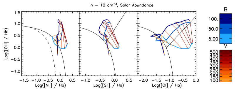
Figure 4.— Shock grids (Allen et al., 2008) are presented for a solar abundance with $n_{e}$ = 10  cm^-3. The yellow - orange lines are contours of constant shock velocity in  km s^-1. The cyan - blue lines are lines of constant magnetic field in $\mu$G. Also included in the plots are the “extreme starburst lines” and the lines that indicate the distinction between Seyferts and LINERs. Larger forbidden to Balmer line ratios can indicate either a faster shock, or a larger contribution by AGN. In Appendix A we present these diagnostics along with the individual line ratios for each component in each galaxy.

The clearest cases for grouping a component into “shock-like” or “HII-like” is when all three diagnostic measurements (log([O III]/H$\beta$) versus log([N II]/H$\alpha$), log([S II]/H$\alpha$) and log([O I]/H$\alpha$)) agree, i.e., are below or above this extreme starburst line. In cases where the measures do not agree, we generally rely upon the sensitivity of the [O I] transition to determine the classification for a particular component. For cases where the errors in flux ratio are consistent with either case, we classify the component as “unclear”. For each galaxy, we present the emission line ratios for each component on these diagrams in Appendix A.

4. Location of Shocked Gas

The categorization of emission into different excitation categories allows the identification of “shock-like” ratios beyond the nuclei of the galaxies. For the 38 galaxies that exhibit “shock-like” emission line ratios in at least one of the components, the spatial position of the “shock-like” component lies 3 kpc from the nucleus. For 14 of the objects, “shock-like” emission also appears within 2 kpc of the nucleus. Only one galaxy shows exclusively “HII-like” emission – IRAS16474+3430.

The kinematic spatial variations along the slit suggest that some of these galaxies host gas disks, despite disturbance caused by the merger interaction. The smooth transition of Doppler shift from red to blue identifies the candidate disks, while the excitation categories indicate that gas with “shock-like” excitation share the same kinematics. We define a “disk” in these cases as when the contiguous components with $\sigma_{v}<150$  km s^-1 cross the line $v=0$  km s^-1. We make an exception in the cases where two nuclei are present, as indicated by the presence of a second continuum peak. In these cases, the objects have motions associated with their interaction, so are allowed to have a velocity offset. Using these parameters, we find 12 systems with clear disks, presented in Figure 5 and described in Section 4.1.1. We include the measured rotation gradients in Table 3.

4.1. Evidence for Gas Disks

4.1.1 Individual Objects

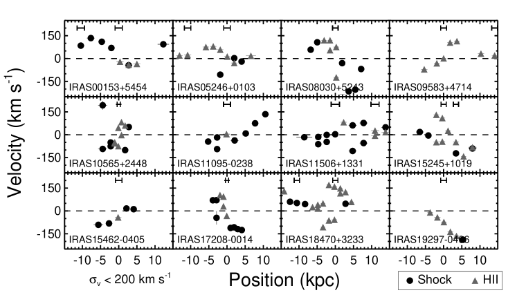
Figure 5.— In the above plot we show position-velocity diagrams for components with $\sigma_{v}<200$  km s^-1 for 12 objects with profiles most indicative of rotation. We identify nuclei based on the position of continuum sources in the 2D spectra, which are marked above the data points. In IRAS00153+5454, IRAS11095-0238, and IRAS15462-0450 the shocked components appear to be part of a rotating gas disk. IRAS05246+0103, IRAS08030+5243, IRAS09583+4714, and IRAS19297-0406 on the other hand, present predominantly HII-like emission in its gas disk. IRAS17208-0014 and IRAS18470+3233 show a mixture of HII and shock, with the shock in the outer edges of the disk. IRAS11506+1331, IRAS18470+3233, and IRAS 15245+1019, are double nucleus objects with possibly multiple disks, and a large mixture of HII and shock excitation.

IRAS00153+5454 - Fig. A2 shows two continuum sources, identifying it as a double nucleus object with a separation of $\sim$ 10 kpc. The emission for the northern nucleus is dominated by “shock-like” emission, while a smaller shock region exists in the southern nucleus. The velocities in the northern nucleus may incdicate rotation in a disk.

IRAS01298-0744 - The emission in this object extends to $\sim 12$ kpc from the continuum source. Rotation is evident in the central and northern regions of the disk (Fig. A6), while the emission in the far south presents more of a flat rotation profile. Apertures 4 and 5 in Fig. B6 show a peculiar emission component on the red side of the H$\alpha$+[N II] line profile. This emission is not fit, since it does not clearly show up in any of the other transisitions.

IRAS03158+4227 - The narrow components are primarily “shock-like”, and only shows a shallow rotation gradient in Fig. Fig. A7. The morphology of the $r$ band image is consistent with a face on disk-like objects, which could explain the flat rotation curve.

IRAS05246+0103 - This double nucleus object is spatially extended by approximately 11 kpc, however they both appear to have extended gas disks. The extended emission is mostly dominated by “HII-like” emission. In the position-velocity plot (Fig. A9) shows two disk-like rotation curves with broader emission closer to the nuclei. The narrow emission lines in these cases is more often HII-like, but some components at the East side of the eastern nucleus have shock-like line ratios. In the line profile plots (Fig. B9), apertures 4 and 6 show a good example of the simultaneous fitting decomposing a blended H$\alpha$+[N II] profile.

IRAS08030+5243 - one of the clearer examples of disk associated rotation, which includes narrow “shock-like” emission. At the far ends of this rotation curve (Fig. A10) in this object the Doppler shift turns around and approaches the systemic velocity. The central aperture in this case shows a double peaked narrow emission profile (Fig. B10), where the apertures outside of this have more clear broad profiles.

IRAS08311-2459 - The gas disk in this object emits both “HII-like” and shock-like emission at distances up to 4 kpc from the continuum source. In this case the rotation (Fig. A11) in narrower emission lines is clear compared to the broad emission line profiles, which are at a constant Doppler shift of $\sim 50$ km s^-1along the slit. The diagnostic diagrams in this case show strong [O III]/H$\beta$ ratios, however the [O I] in this case is unmeasured due to flaws in the data files.

IRAS09111-1007 - The rotation in this object shifts from -50  km s^-1 to 100  km s^-1 showing that this object may host a disk (Fig. A12). The disk components are comprised equally of “HII-like” and “shock-like” emission components. In the center few apertures there are strongly blueshifted components relative to the velocities of the disk.

IRAS09583+4714 - One of the clearest examples of disk associated rotation appears in Fig. A13. Two nuclei are present, however the eastern nucleus exhibits strong rotation, while the western nucleus is mostly a flat rotation curve. The rotation curves are a comprised of “HII-like” emission components. For this object we do not have an $r$ band image to compare to the 2D spectroscopy, which makes the interpretation slightly more difficult.

IRAS10565+2448 - This lower redshift object shows that the disk rotation (Fig. A16.) is complex, however there is again a trend from red to blue ($\pm 100$  km s^-1) indicating possible rotation in a disk. the further extended components are “shock-like” in this case.

IRAS11095-0238 - The rotation in this object has a larger extent on one side of this object (Fig. A17). The emission lines are dominated by “shock-like” emission through out the object, mostly appearing in the LINER region of the diagnostic diagrams.

IRAS11506+1331 - Two disks are resolved in Fig. A18 for this object, where the gas between the two nuclei are separated in velocity space by $\sim 150$  km s^-1. Most of the gas in the object emits “shock-like” emission, again in the LINER region of the diagnostic diagram.

IRAS11598-0112 - The emission line profiles in this object are generally more chaotic, however, the narrow part of the line profile presents a general red to blue trend in Fig. A19 over a wide spatial ($\pm 8$ kpc) and velocity. The fits in Fig. B19 had some difficulty capturing the line profile in aperture 0.

IRAS15245+1019 - This ULIRG has double with nuclei separated by $\sim$ 4kpc, as shown in Fig. A1. It is difficult to distinguish which galaxy each of the components belongs to, since they span the same spatial range, however, in either interpretation there appears to be two disks involved.

IRAS15462-0405 - Narrow emission shows a disk like rotation profile in Fig. A1, though the broad part of the line profile behaves much differently than the rest of the objects.

IRAS16487+5447 - This object is a double separated by 5 kpc with a complicated position- velocity diagram (Fig. A26). There are two extended emission components, however, and the narrower emission component presents more disk like rotation.

IRAS17208-0014 - This object is a double, separated by $\sim$ 2 kpc. In Fig. A28 The rotation seems to cross the two nuclei with the north side having a flat rotation profile at -100  km s^-1, and the south side more chaotic.

IRAS17574+0629 - The position-velocity diagram (Fig. A29) separates the two galaxies in velocity space, revealing two separate disks. The morphology of the $r$ band image gives some indication that the merging disks may be nearly orthogonal or a multiple merger. The emission in this collision is dominated by “HII-like” emission.

IRAS18470+3233 - This object is a multiple merger. In Fig. A32 the western galaxy in this merger hosts two emission features that present “disk-like” line profiles separated by a 150  km s^-1offset. The eastern galaxy has a spatially large rotation profile, which includes shock inoization in the central 4 kpc.

IRAS19297-0406 - This object presents rotation profiles in Fig. A33 that extend to $\pm 5$ kpc and are mostly “HII-like” in ionization. The whole rotation curve is offset from systemic, implying that there is a possible slight error in the used redshift.

IRAS20046-0623 - The continuum profile in this object is flat along the spatial axis and extended over 8 kpc as can be seen in the 2D spectrum of Fig. A35. There are no clear peaks in the continuum profile. The $r$ band image indicates that the two intersecting galaxies are nearly perpendicular. A rotation gradient is evident along the major axis of the sampled objects, while the minor axis shows little rotation.

Table 3 Disks

IRAS Name	Edge Positions		$v_{rad}$		rotation grad
	kpc		km s-1		km s-1 kpc-1
(1)	(2)	(3)	(4)	(5)	(6)
00153$+$5454(a)	-10.3	-2.2	79	133	2.1
00153$+$5454(b)	0.2	11.9	-45	93	10.5
01298$-$0744	-10.6	3.9	-34	28	3.1
03158$+$4227	-6.7	9.6	-17	35	2.0
05246$+$0103(a)	-5.8	6.6	-105	79	5.6
05246$+$0103(b)	-13.1	-8.7	16	23	1.0
08030$+$5243	-3.6	3.7	-348	461	73.8
08311$-$2459	-4.1	4.3	-131	56	24.9
09111$-$1007	-4.2	7.4	-115	113	11.6
09583$+$4714	-5.3	3.7	-70	114	22.6
10565$+$2448	-4.4	2.8	-101	193	0.7
11095$-$0238	-5.2	10.6	-94	134	11.3
11506$+$1331(a)	-8.5	7.8	-62	283	9.1
11506$+$1331(b)	4.8	13.8	-106	48	15.6
11598$-$0112	-5.2	10.4	-192	336	-23.6
15245$+$1019	-6.6	7.9	-142	131	11.3
15462$-$0405	-5.6	4.1	-91	16	12.5
16487$+$5447	-8.3	7.2	-294	28	15.8
17208$-$0014	-4.6	4.6	-127	143	32.4
18470$+$3233(a)	-4.8	4.4	-106	170	11.1
18470$+$3233(b)	-15.7	-6.3	25	147	12.8
19297$-$0406	-6.4	5.8	-192	43	19.8

Note. — Col.(1):IRAS name; Cols.(2&3): Distance of the rotation profile edge from the continuum source in kpc; Cols.(4&5): Minimum and maximum velocities of rotation profile in  km s^-1. Col.(6): Rotation gradient in  km s^-1 kpc^-1.

4.1.2 Conclusions

Out of the entire sample of 39 ULIRGs, the twenty objects in Sect. 4.1.1 are the ULIRGs with candidate gas disks. These candidate gas disks have narrow emission lines with $\sigma\leq 150\mbox{~{}km~{}s${}^{-1}$}$ that vary smoothly in Doppler shift along the slit. The remaining objects in the sample have either little evidence of an extended gas, broader emission features, or unclear spatial trends in the gas kinematics. Four objects out of the full sample (IRAS03521+0028, IRAS10378+1109, IRAS16090-0139,IRAS18368+3549) exhibit only less ordered motion that is not clearly part of a disk.

The sample included in this study chooses galaxies at various merger phases, which we can compare to the presence of a rotation profile in the position velocity diagrams. Twelve objects with the clearest rotation profiles presented in Fig. 5 show strong gradients in Doppler shift along the slit. In this representative set of twelve ULIRGs, seven are in binaries, one is a multiple merger, and the remaining four are at a later single nucleus phase with extended diffuse emission. The number of early merger phase objects with clear disks suggests that a gas disk appears at early stages of the merger, then removed as the galaxies coalesce.

Spatially resolved emission line diagnostics allow us to examine the relationship between the presence of rotation and the spatial distribution of gas excitation. Two disks appear in some of the double nuclei objects, increasing the number of disks to consider to 15. IRAS05246+0103, IRAS19297-0406, IRAS09583+4714, IRAS15245+1019 and IRAS18470+3233 show disks that are strongly dominated by HII-like excitation. In IRAS11095-0238, both disks in IRAS11506+1331, IRAS15462-0405, and IRAS00153+5454 the rotating gas is dominated by shock-like excitation. The remaining 5 disks (IRAS08030+5243, IRAS10565+2448, IRAS15245, IRAS17208-0014, and IRAS18470+3233) are evenly mixed in both HII-like and shock-like excitation. The distribution of excitation in these objects places the HII-like regions closer to nuclei, with shock-like excitation in the outer few kpc, with an exception for IRAS18470+3233. This HII-centered distribution also appears in the shock dominated disks, where just the central aperture is HII-like, but the rest of the disk is dominated by shock-like excitation. The distribution of excitation however is not clearly related to the merger class in this subsample.

There are at least 4 different possible origins of narrow shocked components of the emission line profiles. (1) In merger models (Cox et al., 2004), shocks occur as the gas disks collide. (2) Shocks also occur as gas that was previously removed via tidal stripping falls back into the galaxies. (3) Shocks can also be produced by the dissipation of energy injected by massive stars created in the burst of star formation. (4) Shock-like emission can also be produced by photoionization via aging post-AGB stars. The gas disks in this study, however, appear more frequently in the earlier, binary stages of the merger. This suggests that the earlier stages of the merger can trigger shocks, rather than only appearing after the galaxies have coalesced.

We stress, however, that the complicated gas kinematics present at all stages of the merger are often difficult to discern with long slit measurements and imaging data. One situation that leads to confusion is that some velocity profiles do not reach the same maximum velocity in both directions along the slit from the nucleus. Additionally, the orientation of this gas disk with respect to the line of sight is not clear, meaning that objects with a shallow rotation gradient may simply be close to face-on, thereby decreasing the line of sight velocity. Furthermore, the slit position angle was selected to either sample multiple nuclei or sample an elongation in the $r$ band image of the object, so a possible misalignment with the major axis would interfere with the detection of a disk.

Future observations that employ integral field spectroscopy will allow a better analysis of the gas kinematics and excitation in concert with its spatial distribution along the merger sequence. Spatial continuity in these types of measurements allow a better understanding of larger scale features such as disk inclination, as well as isolating regions of varying excitation. Better measurement of the kinematic features can further better estimates of merger phase and lead better understanding of the processes that create shocked gas disks.

5. Summary

In this analysis of longslit ESI data, we observed complex line profiles in the various line species used for the examination of emission line excitation. The spectral resolution and signal to noise obtained with ESI allow detailed investigation of the underlying emission mechanisms. Spatial resolution along the long slit allows us to further understand the extended structure of these sources. By performing a simultaneous multicomponent fits to the Balmer and forbidden lines, we were able to identify shocked gas disks at early merger stages. These data are relevant for many investigative purposes such as informing model creation and examination of gas processes in the merging galaxies and strong star formation environments.

Appendix A Appendix A

In this Appendix we include the figures that represent the spatial distribution, kinematics and excitation from the entire suite of measurements in the full sample. The combination of these plots in the figure set help to illustrate the variations throughout the ULIRGs. The emission line profiles for the measured transitions are presented in Appendix B.

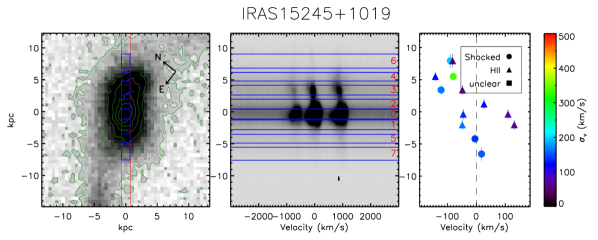
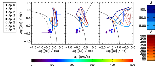
Figure 1.— Top Left: An $r$ band image from the Palomar 60 inch telescope. The green contours represent the median, and the 1, 2, 3, 4, and 5 $\sigma$ surface brightness levels in the image. The red lines show the spatial position of the 1″$\times$20″ slit. The blue rectangles identify the positions of the selected apertures. Top Middle: The 2D spectrum of H$\alpha$+[N II] centered in velocity space on H$\alpha$. The blue rectangles identify the pixels that contribute to the individual apertures. The redshift range of the sample allows each object to be sampled by several apertures along the slit. Top Right: The position-velocity diagram for all of the fit components. The linewidth of the components is indicated by the color of the plot point. The plot symbol represents the excitation category for that individual spectral component. Bottom Row: Line ratio diagrams showing the line ratios for the emission components in these selected apertures. The black solid line represents the extreme star formation limit, above which the excitation mechanism in not expected to be from star formation (Kewley et al., 2006). The dashed line in the [O III]/H$\beta$ vs [N II]/H$\alpha$ represents the empirical star formation limit (Kauffmann et al., 2003a). Shock grids (Allen et al., 2008) are presented for a solar abundance with (blue and orange lines) with $n_{e}=10~{}{\rm cm}^{-3}$, with a velocity range of 100 to 500  km s^-1, and magnetic field strength 5 to 100 $\mu$G expected for star forming galaxies. Overplotted on these diagnostics are flux ratios from the individual components in the apertures identified in the above plots. The full sample is included in the online version of the article.

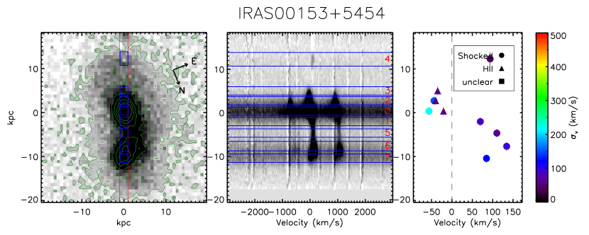
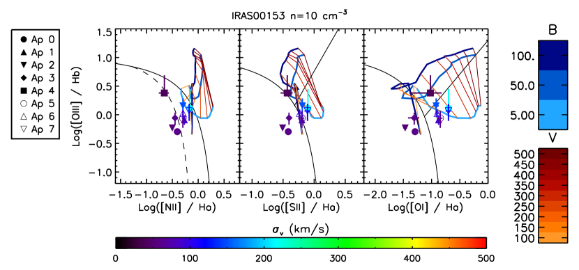
Figure 2.—

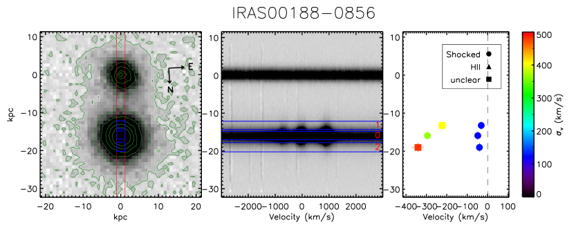
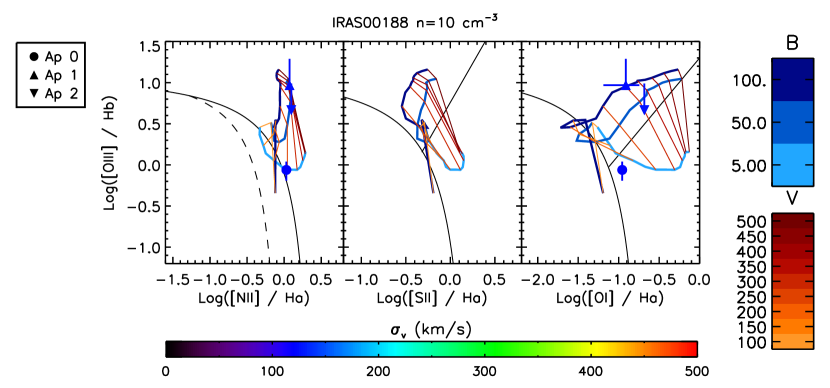
Figure 3.—

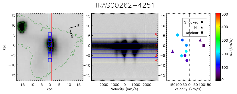
Figure 4.—

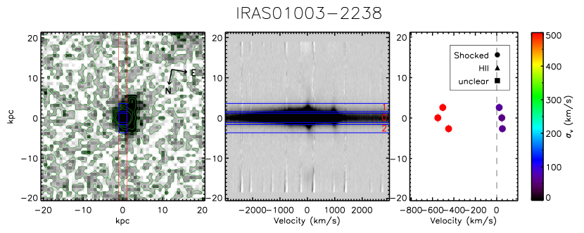
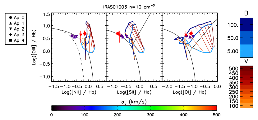
Figure 5.—

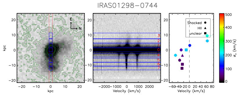
Figure 6.—

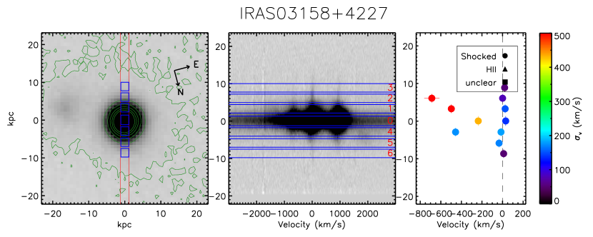
Figure 7.—

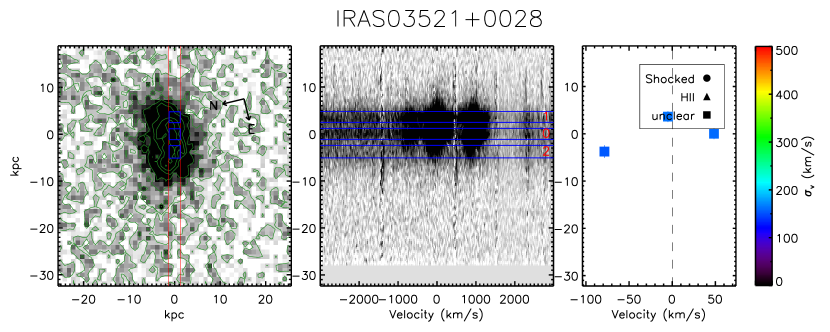
Figure 8.—

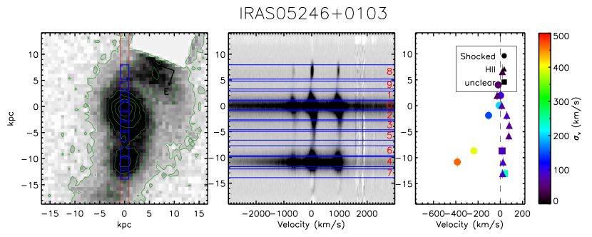
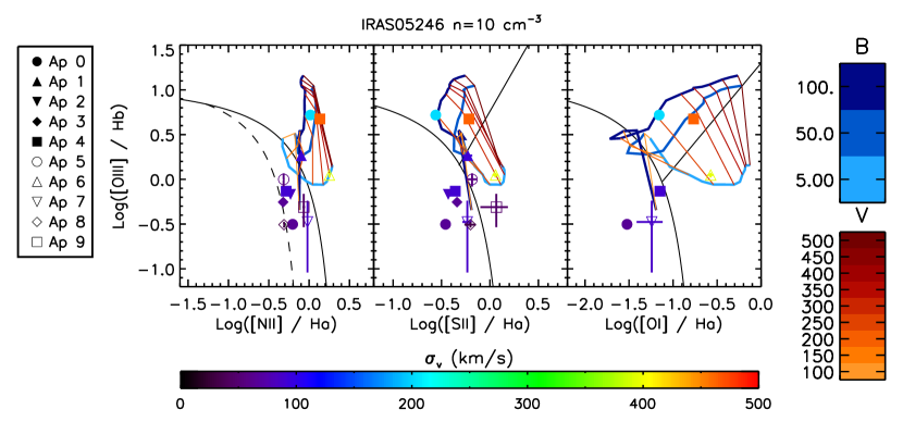
Figure 9.—

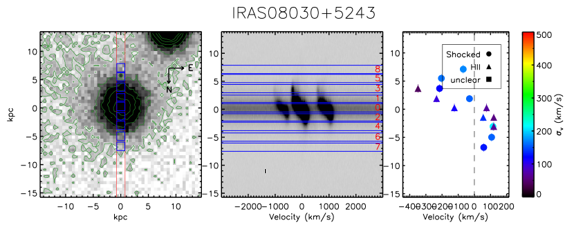
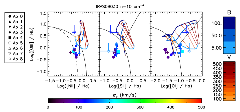
Figure 10.—

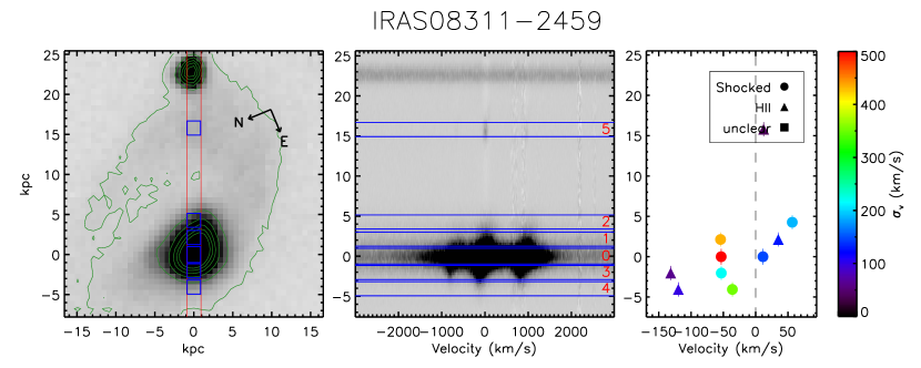
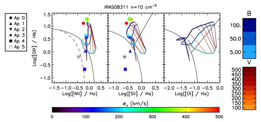
Figure 11.—

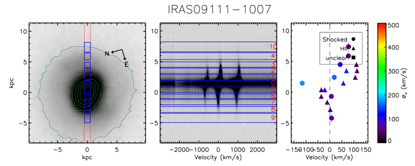
Figure 12.—

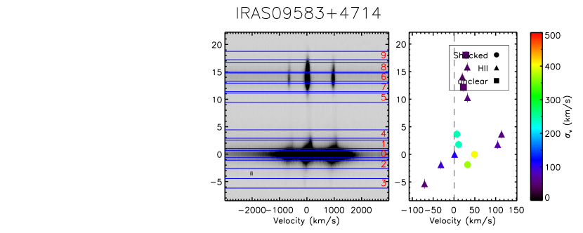
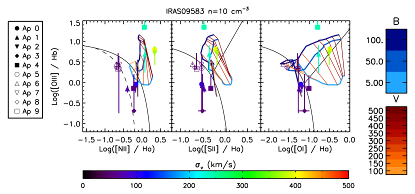
Figure 13.—

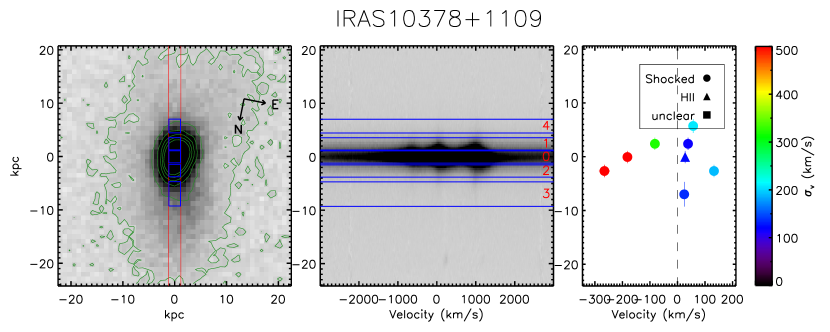
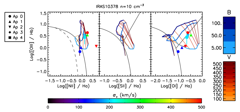
Figure 14.—

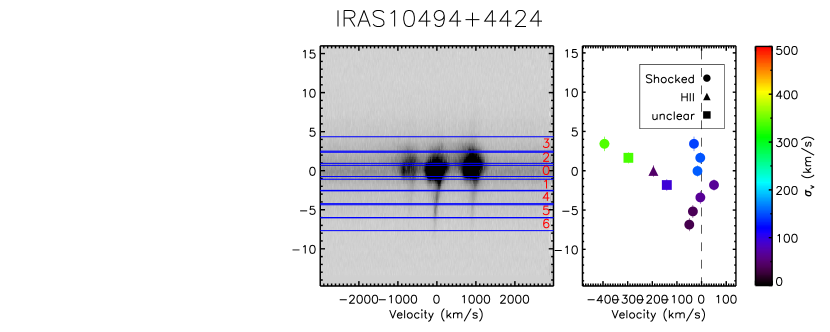
Figure 15.—

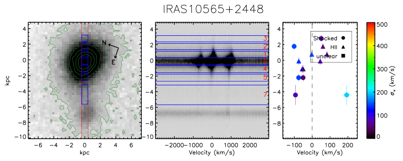
Figure 16.—

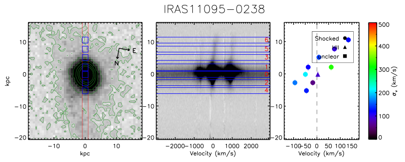
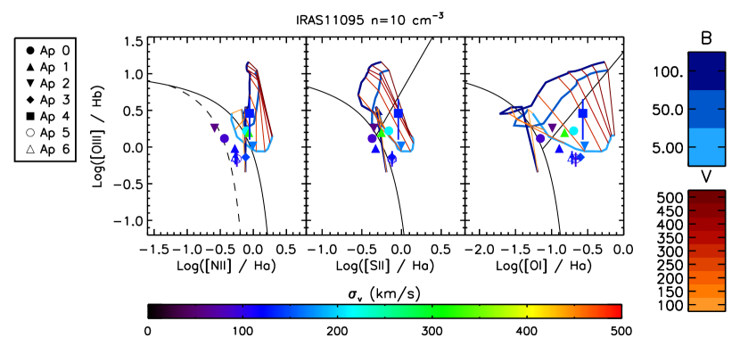
Figure 17.—

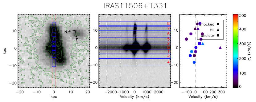
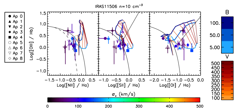
Figure 18.—

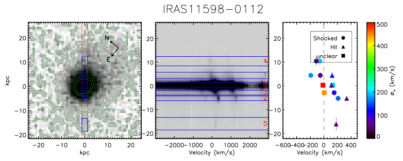
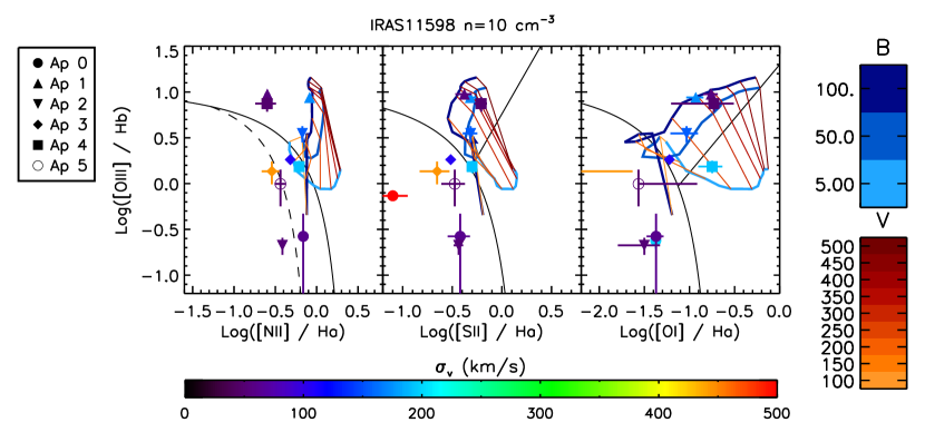
Figure 19.—

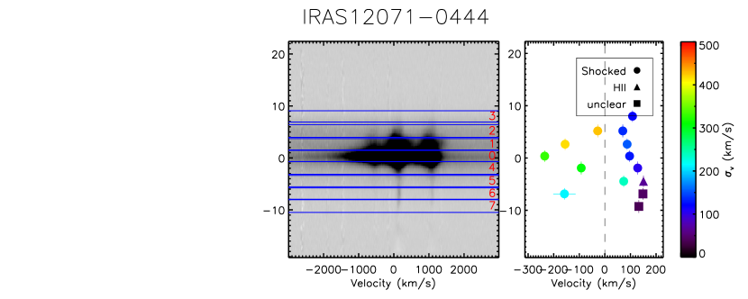
Figure 20.—

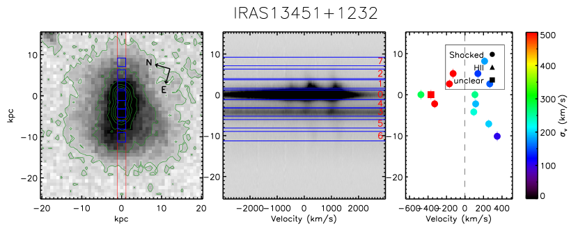
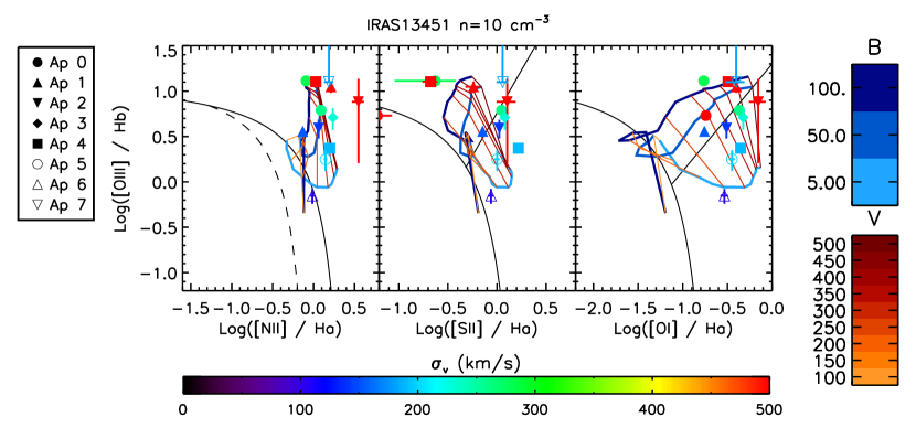
Figure 21.—

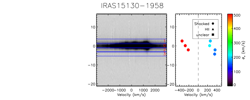
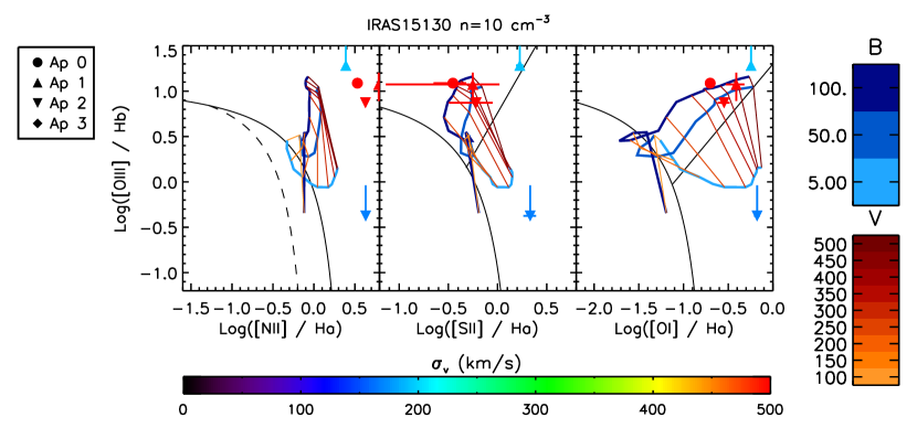
Figure 22.—

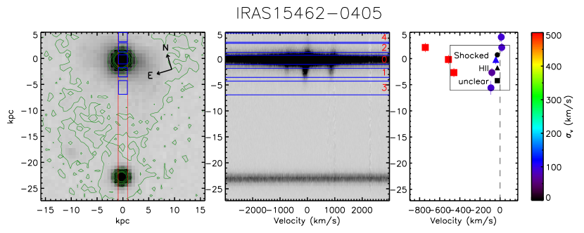
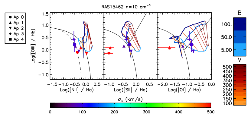
Figure 23.—

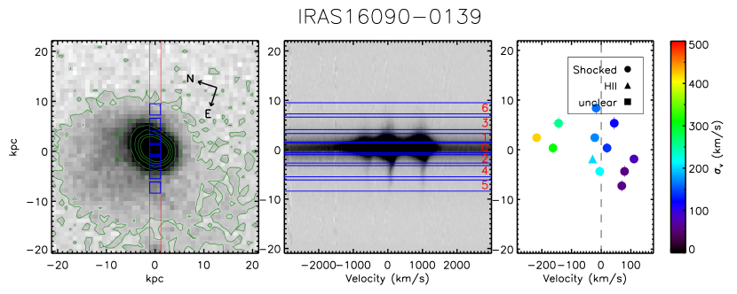
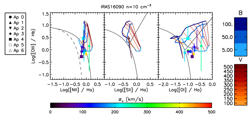
Figure 24.—

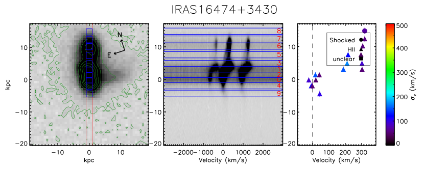
Figure 25.—

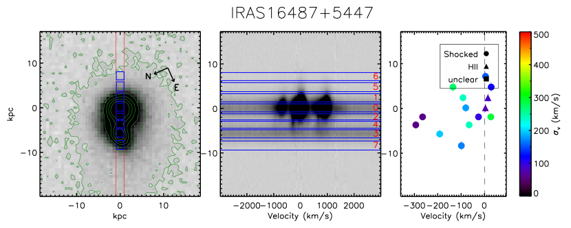
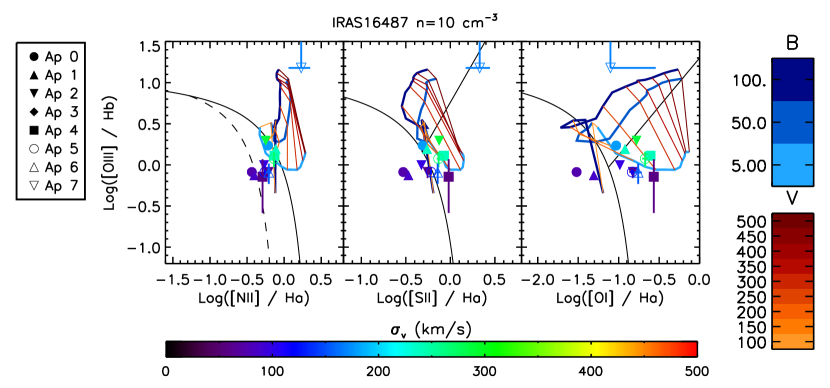
Figure 26.—

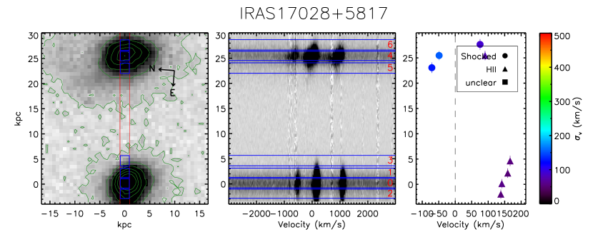
Figure 27.—

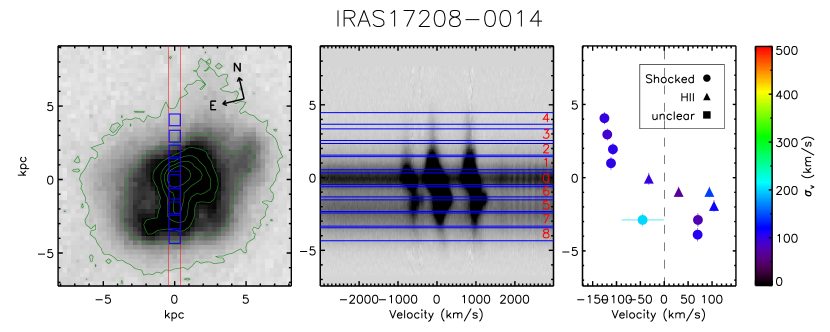
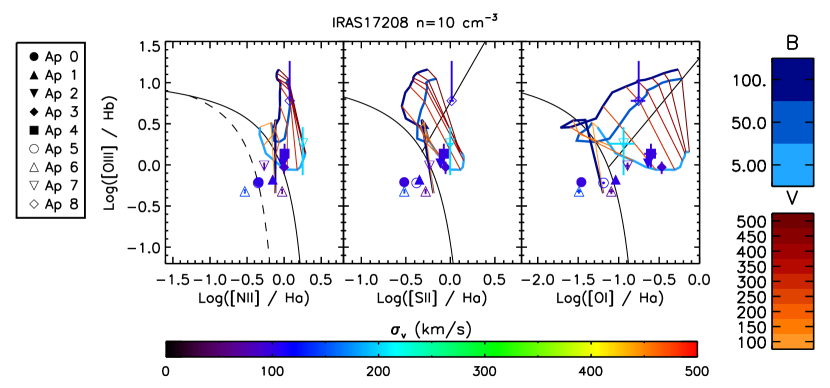
Figure 28.—

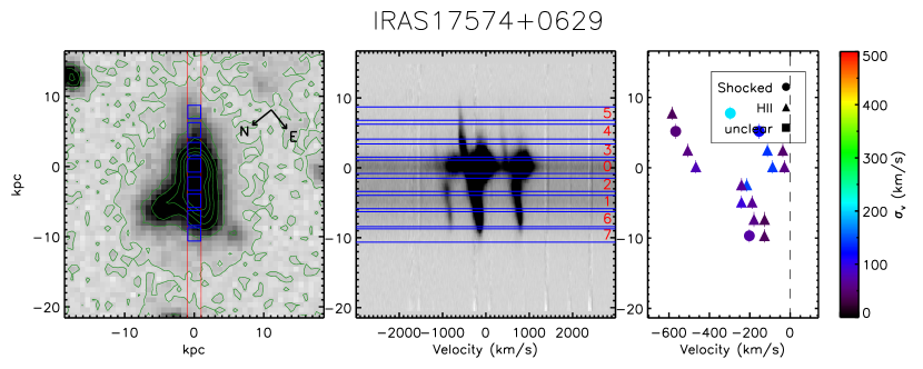
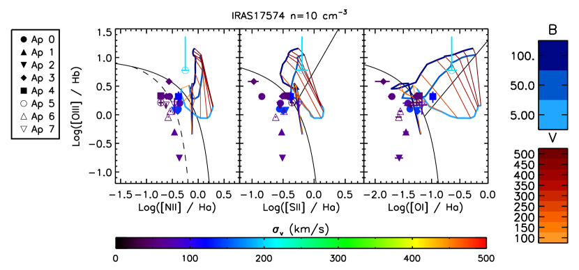
Figure 29.—

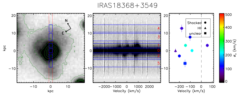
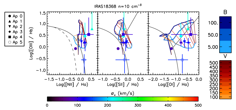
Figure 30.—

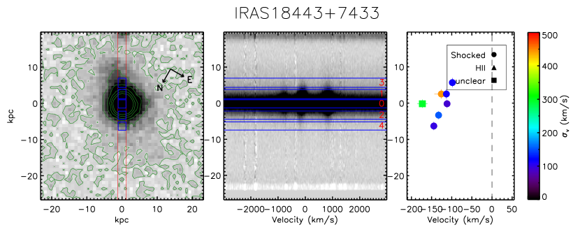
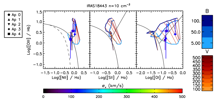
Figure 31.—

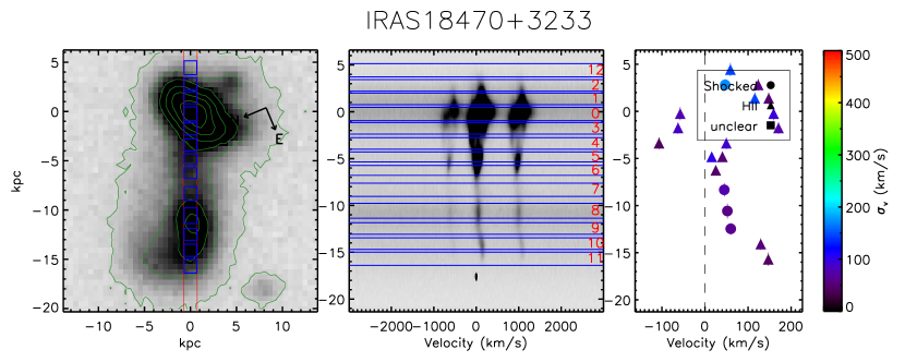
Figure 32.—

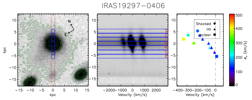
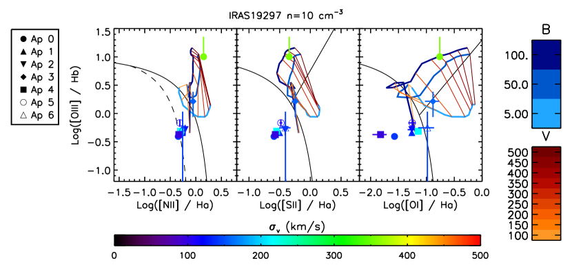
Figure 33.—

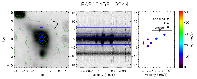
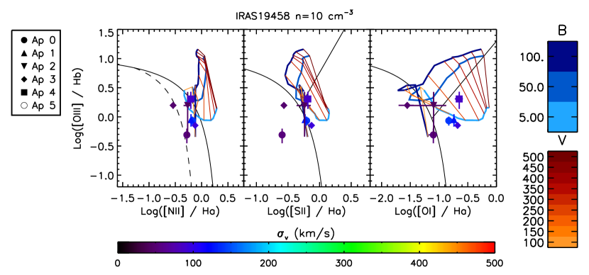
Figure 34.—

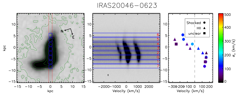
Figure 35.—

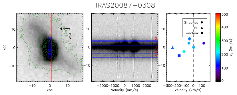
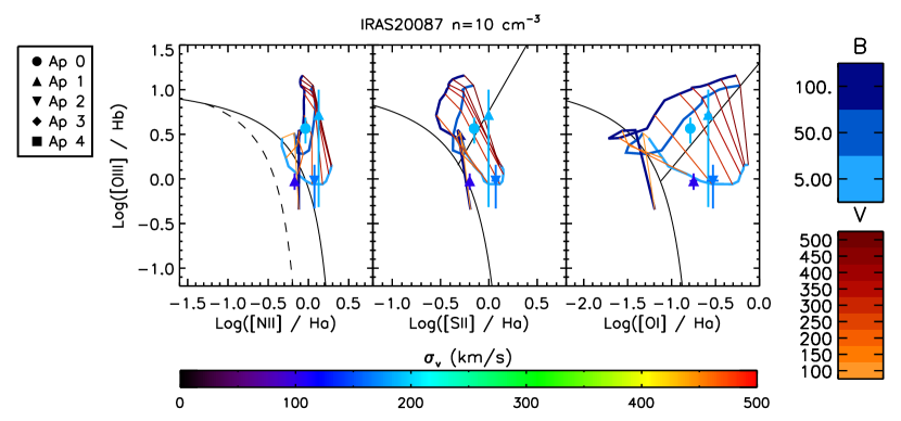
Figure 36.—

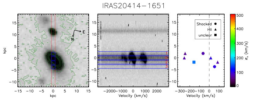
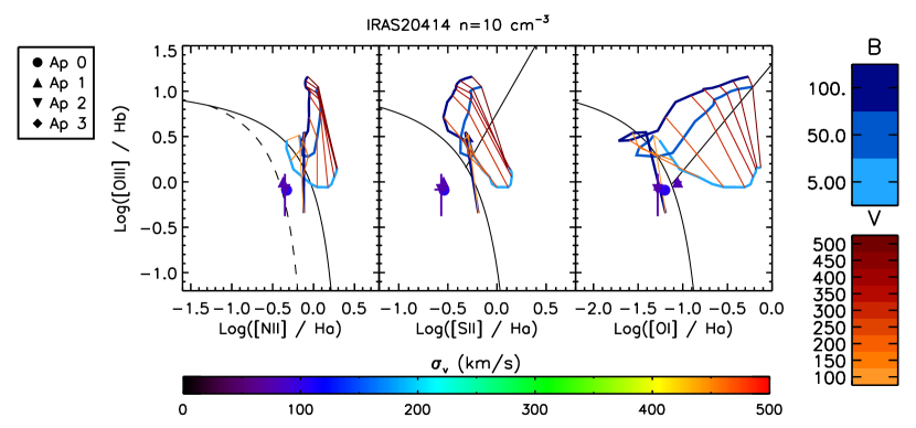
Figure 37.—

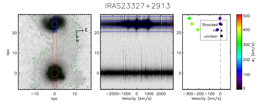
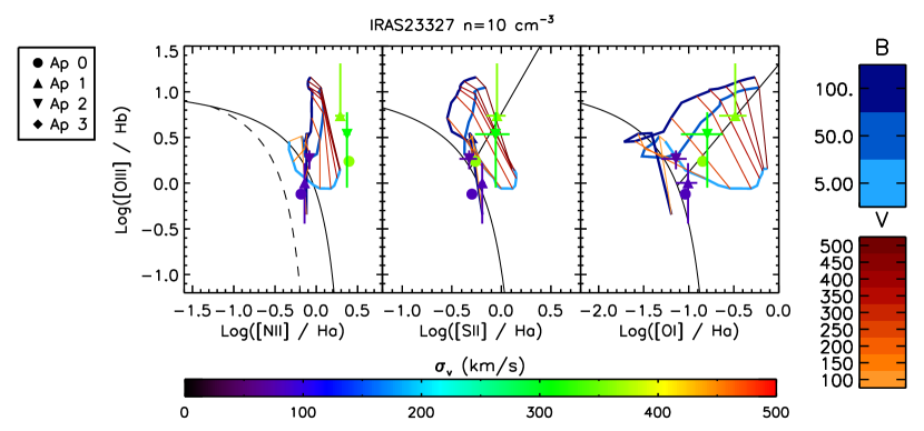
Figure 38.—

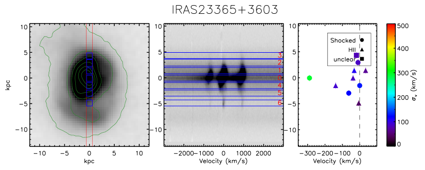
Figure 39.—

Appendix B Appendix B

In this appendix we include the emission line profiles for the transitions identified by the apertures figure set of Appendix A. The measured fluxes and estimated shock velocities from the line ratios are presented in Appendix C.

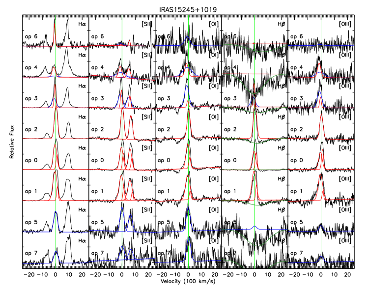
Figure 1.— Line profiles for each measured transition (horizontal axis) as a function of aperture (vertical axis). Each cell is labeled with the transition and and aperture number identified in Fig. 1. The scales have been adjusted to illustrate the line profile in each transition. The red and blue lines identify the different gaussian components from the resulting simultaneous fit. The dark green line represents the H$\beta$ absorption component. For the left column, only the components of the H$\alpha$ transition are displayed to minimize confusion; the [N II] kinematics are the same as the other transitions, while the amplitudes can vary. The full sample is included in the online version of the article.

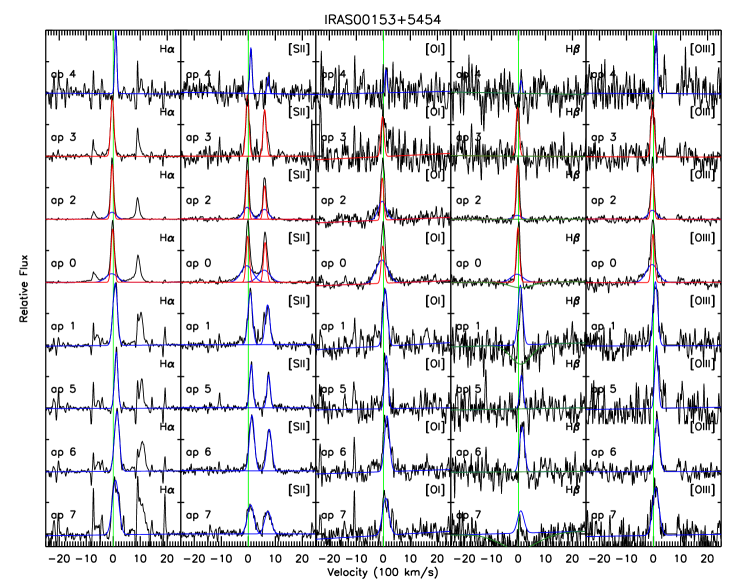
Figure 2.—

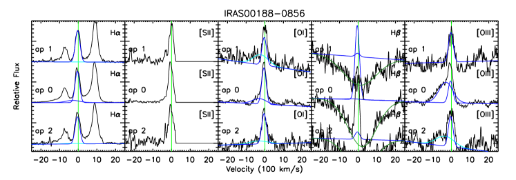
Figure 3.—

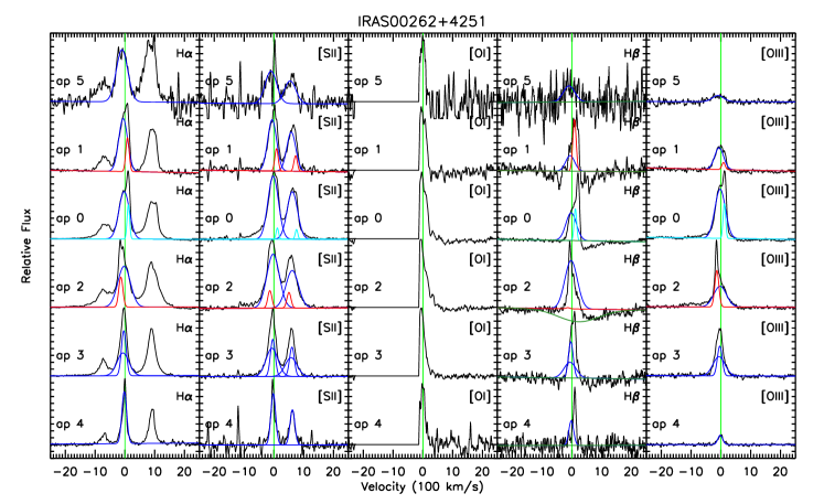
Figure 4.—

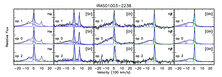
Figure 5.—

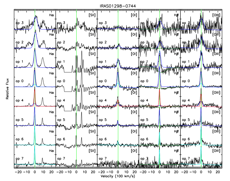
Figure 6.—

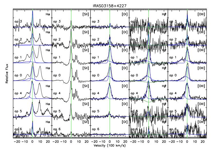
Figure 7.—

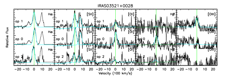
Figure 8.—

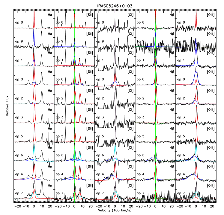
Figure 9.—

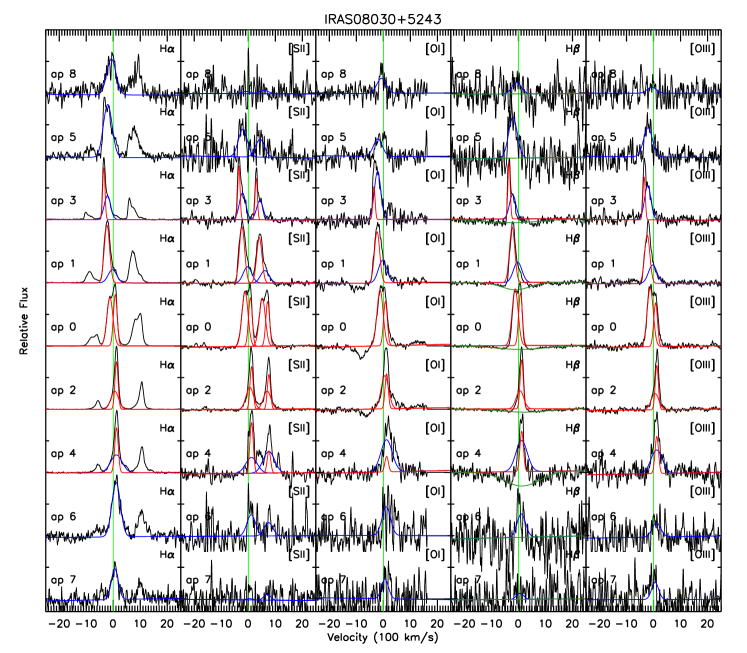
Figure 10.—

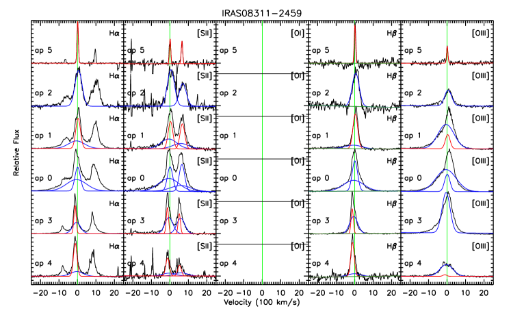
Figure 11.—

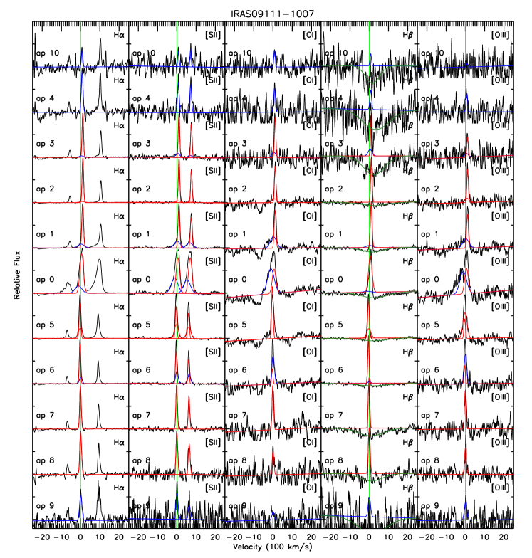
Figure 12.—

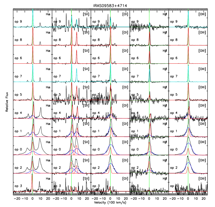
Figure 13.—

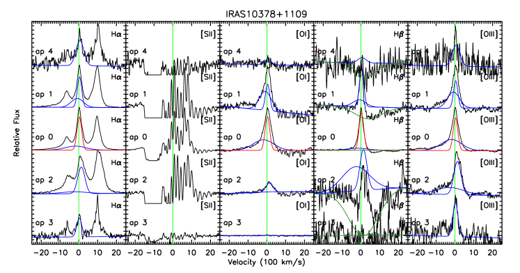
Figure 14.—

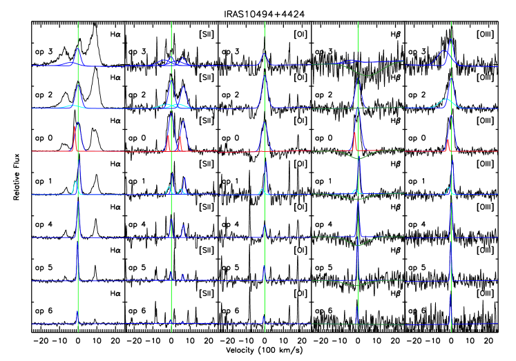
Figure 15.—

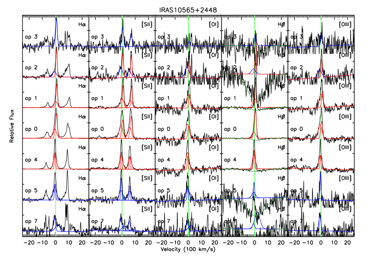
Figure 16.—

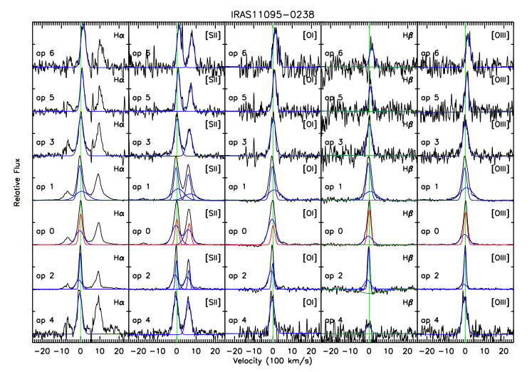
Figure 17.—

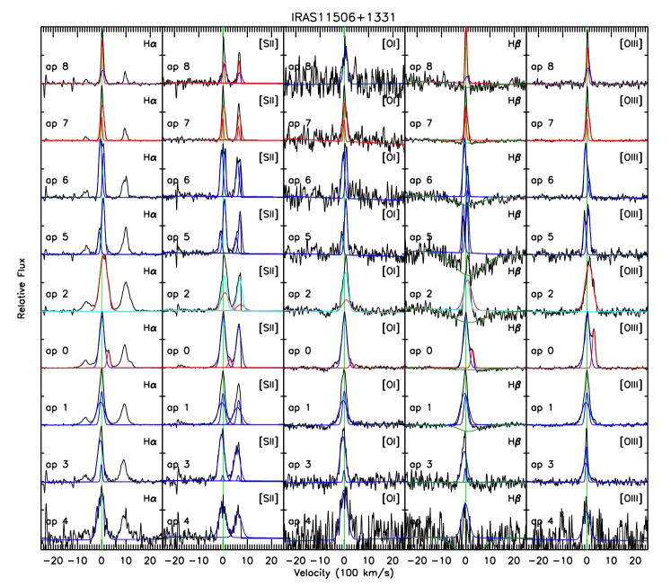
Figure 18.—

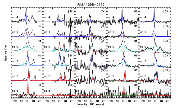
Figure 19.—

Figure 20.—

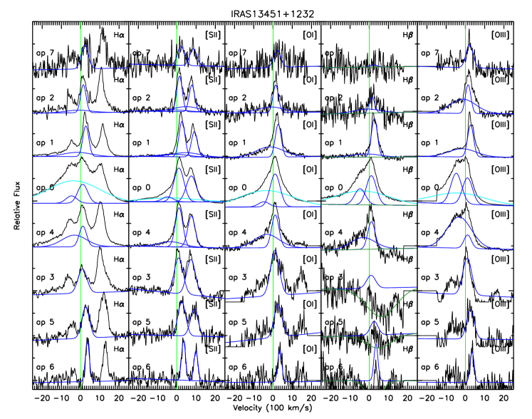
Figure 21.—

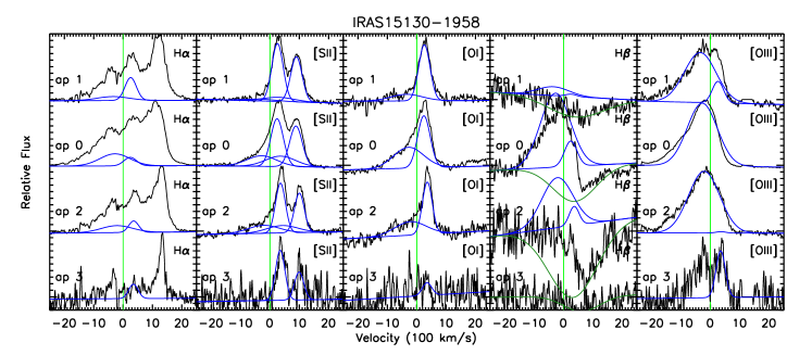
Figure 22.—

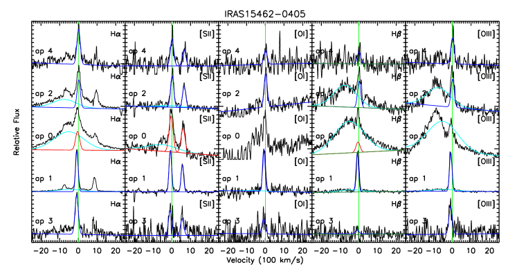
Figure 23.—

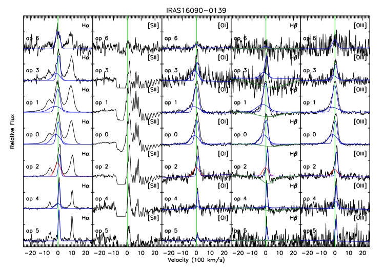
Figure 24.—

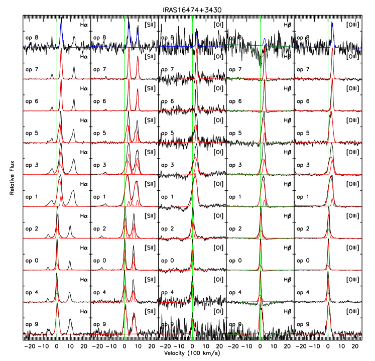
Figure 25.—

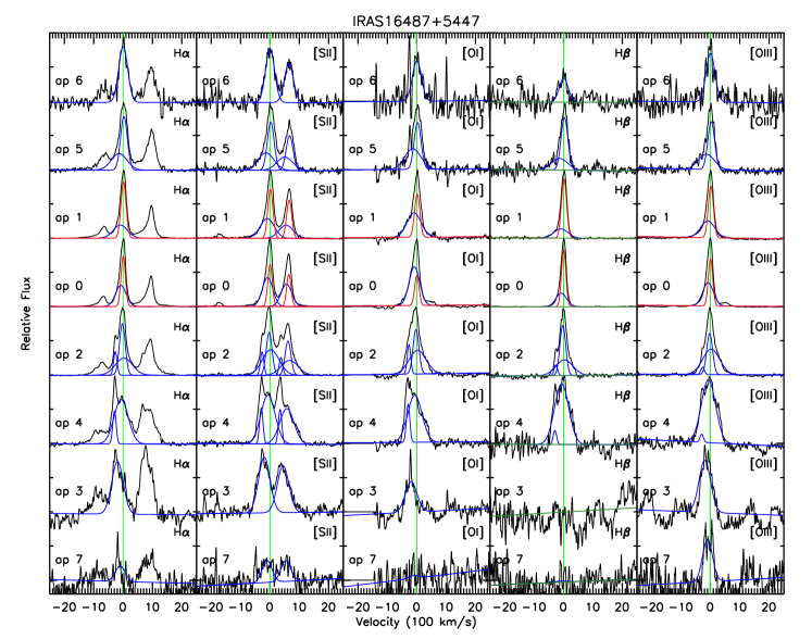
Figure 26.—

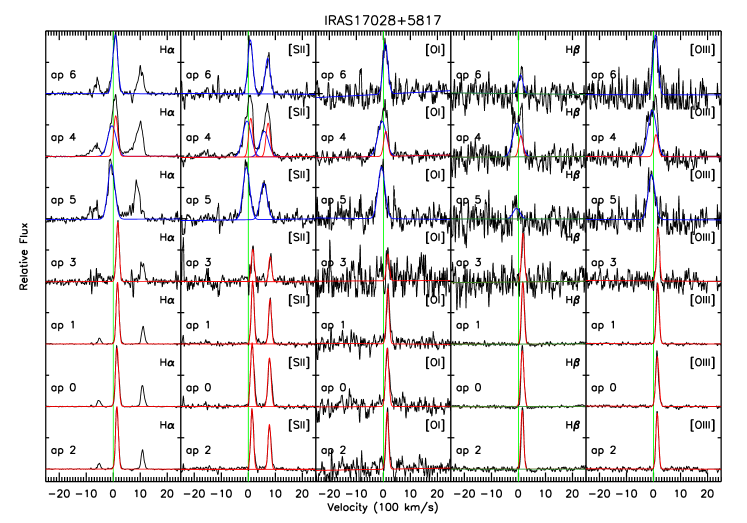
Figure 27.—

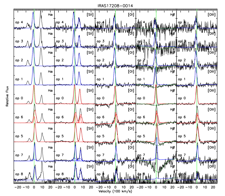
Figure 28.—

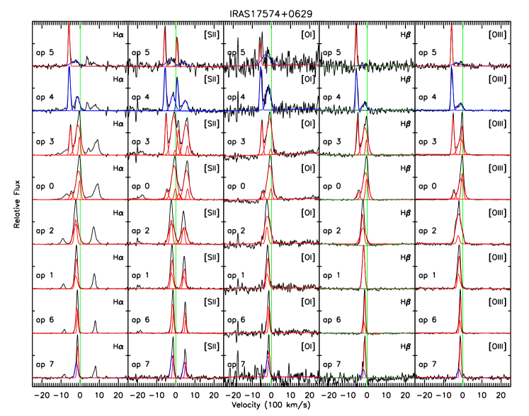
Figure 29.—

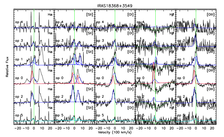
Figure 30.—

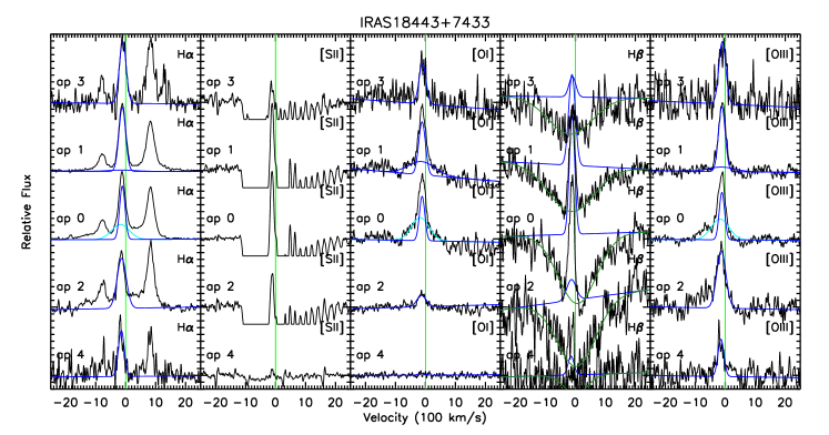
Figure 31.—

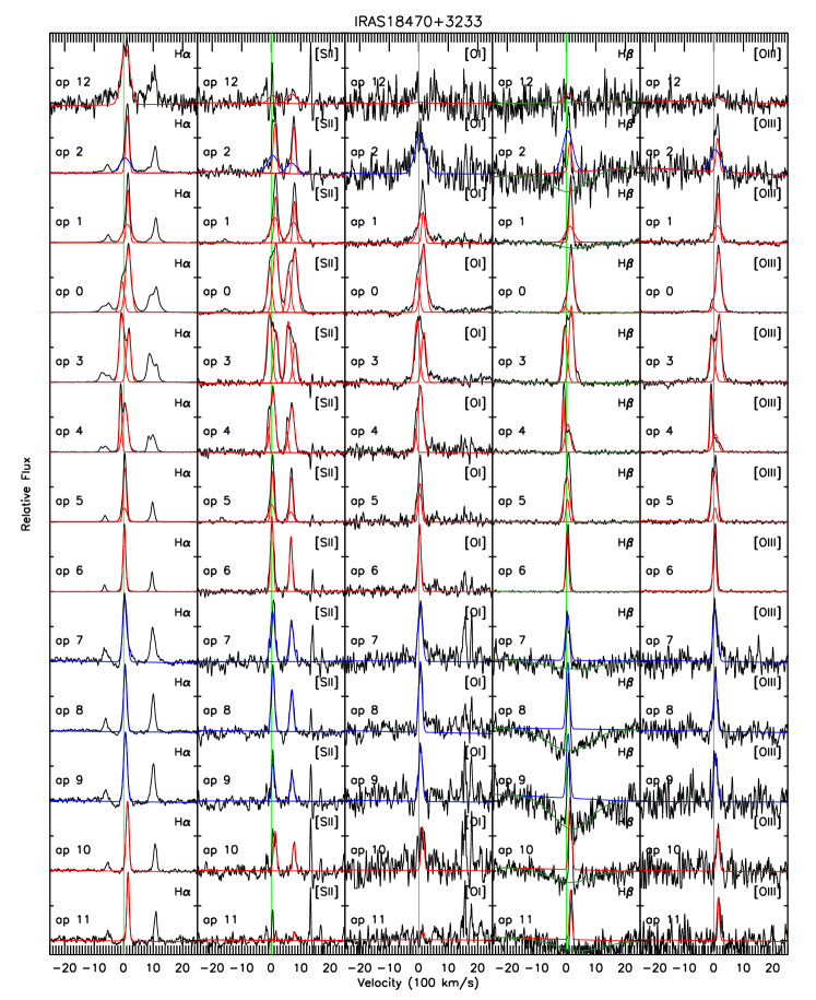
Figure 32.—

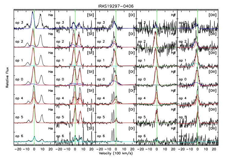
Figure 33.—

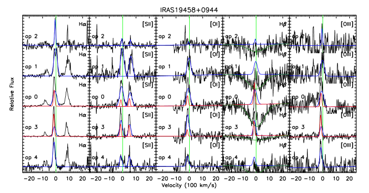
Figure 34.—

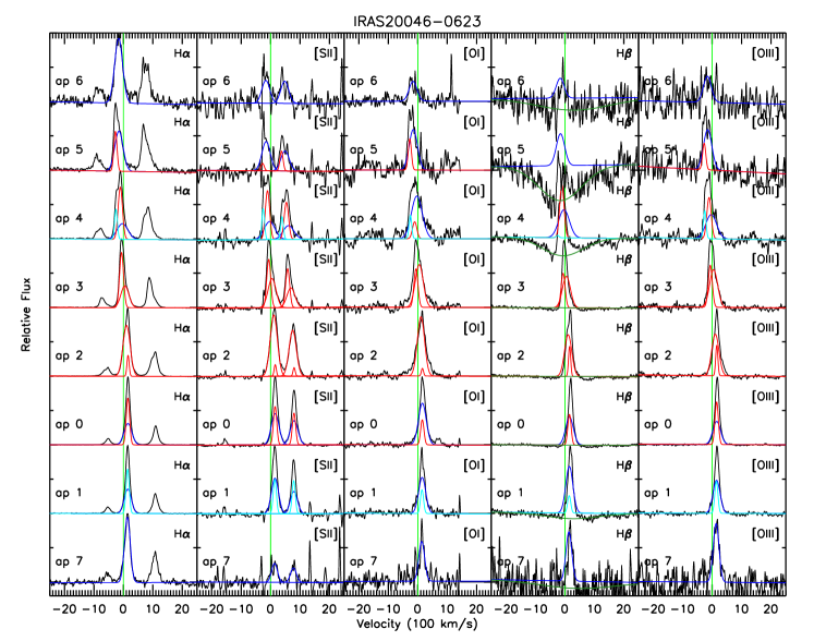
Figure 35.—

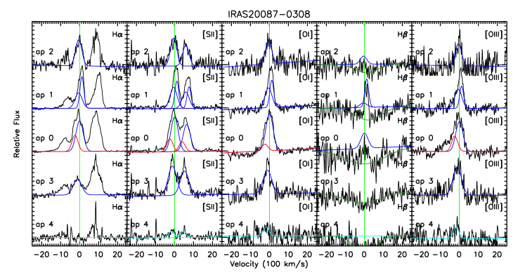
Figure 36.—

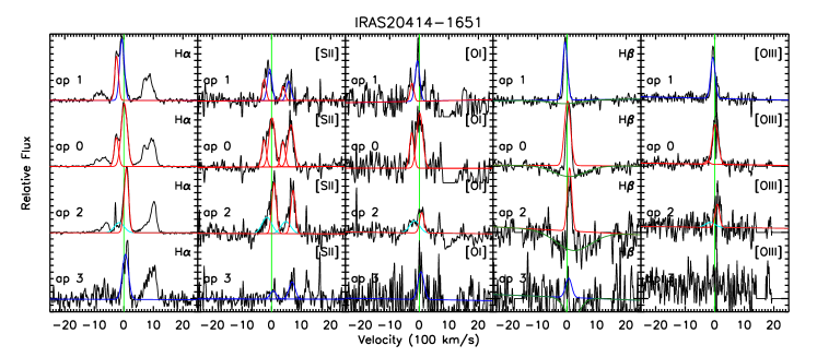
Figure 37.—

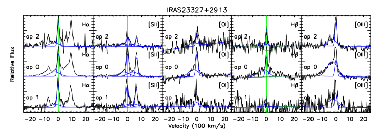
Figure 38.—

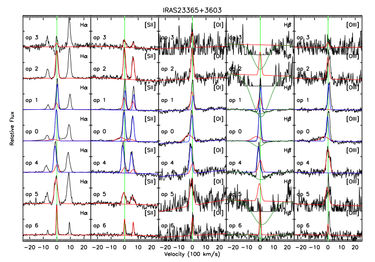
Figure 39.—

Appendix C Appendix C

Note. — Column 1: IRAS galaxy. Column 2: aperture number. Column 3: excitation classification: h denotes a component with HII-like line ratios, s represents components with line ratios indicative of shock, u is an unclear component where the errors in the flux ratio make the measurement consistent with either interpretation. Column 4: distance of sampled region from associated nucleus in kpc. Column 5: size of the selected aperture in kpc. Column 6: Line of sight velocity of fitted spectral component in  km s^-1. Column 7: Velocity dispersion of fitted spectral component in  km s^-1. Column 8: Flux of H$\alpha$ emission in the fitted spectral component in units of 10^-17 erg s^-1 cm^-2. Column 9: Flux of [N II] emission in the fitted spectral component in units of 10^-17 erg s^-1 cm^-2. Column 10: Flux of [S II] emission in the fitted spectral component in units of 10^-17 erg s^-1 cm^-2. Column 11: Flux of [O I] emission in the fitted spectral component in units of 10^-17 erg s^-1 cm^-2. Column 12: Flux of H$\beta$ emission in the fitted spectral component in units of 10^-17 erg s^-1 cm^-2. Column 13: Flux of [O III] emission in the fitted spectral component in units of 10^-17 erg s^-1 cm^-2.

Table 2 Shock Velocities for Identified Shock Components

Note. — Column 1: IRAS galaxy. Column 2: aperture number. Column 3: Line of sight velocity of the fit component in  km s^-1. Column 4: Velocity dispersion of the fit component in  km s^-1. Column 5: velocity of shock front measured from the ratios log([O III]/H$\alpha$) vs log([N II]/H$\alpha$) from shock grids of Allen et al. (2008). Column 6: velocity of shock front measured from the ratios log([O III]/H$\alpha$) vs log([S II]/H$\alpha$) from shock grids of Allen et al. (2008). Column 7: velocity of shock front measured from the ratios log([O III]/H$\alpha$) vs log([O I]/H$\alpha$) from shock grids of Allen et al. (2008).

References

- Allen et al. (2008) Allen, M. G., Groves, B. A., Dopita, M. A., Sutherland, R. S., & Kewley, L. J. 2008, The Astrophysical Journal Supplement Series, 178, 20
- Baldwin et al. (1981) Baldwin, J. A., Phillips, M. M., & Terlevich, R. 1981, Astronomical Society of the Pacific, 93, 5
- Colina et al. (2005) Colina, L., Arribas, S., & Monreal-Ibero, A. 2005, The Astrophysical Journal, 621, 725
- Cox et al. (2004) Cox, T. J., Primack, J., Jonsson, P., & Somerville, R. S. 2004, The Astrophysical Journal, 607, L87
- Dopita & Sutherland (1995) Dopita, M. A., & Sutherland, R. S. 1995, Astrophysical Journal v.455, 455, 468
- Genzel et al. (2011) Genzel, R., et al. 2011, The Astrophysical Journal, 733, 101
- Heckman et al. (1990) Heckman, T. M., Armus, L., & Miley, G. K. 1990, Astrophysical Journal Supplement Series (ISSN 0067-0049), 74, 833
- Henault et al. (2003) Henault, F., et al. 2003, Instrument Design and Performance for Optical/Infrared Ground-based Telescopes. Edited by Iye, 4841, 1096
- Kauffmann et al. (2003a) Kauffmann, G., et al. 2003a, Monthly Notices of the Royal Astronomical Society, 346, 1055
- Kauffmann et al. (2003b) —. 2003b, Monthly Notice of the Royal Astronomical Society, 341, 33
- Kennicutt (1998) Kennicutt, R. C. 1998, Astrophysical Journal v.498, 498, 541
- Kewley et al. (2001) Kewley, L. J., Dopita, M. A., Sutherland, R. S., Heisler, C. A., & Trevena, J. 2001, The Astrophysical Journal, 556, 121, (c) 2001: The American Astronomical Society
- Kewley et al. (2006) Kewley, L. J., Groves, B., Kauffmann, G., & Heckman, T. 2006, Monthly Notices of the Royal Astronomical Society, 372, 961
- Law et al. (2007) Law, D. R., Steidel, C. C., Erb, D. K., Larkin, J. E., Pettini, M., Shapley, A. E., & Wright, S. A. 2007, The Astrophysical Journal, 669, 929
- Lehnert & Heckman (1996) Lehnert, M. D., & Heckman, T. M. 1996, Astrophysical Journal v.472, 472, 546
- Martin et al. (2010) Martin, C., Moore, A., Morrissey, P., Matuszewski, M., Rahman, S., Adkins, S., & Epps, H. 2010, Ground-based and Airborne Instrumentation for Astronomy III. Edited by McLean, 7735, 21
- Martin (1998) Martin, C. L. 1998, The Astrophysical Journal, 506, 222
- Martin (2005) —. 2005, The Astrophysical Journal, 621, 227
- Martin (2006) —. 2006, The Astrophysical Journal, 647, 222
- Monreal-Ibero et al. (2010) Monreal-Ibero, A., Arribas, S., Colina, L., Rodriguez-Zaurin, J., Alonso-Herrero, A., & Garcia-Marin, M. 2010, eprint arXiv, 1004, 3933
- Murphy et al. (1996) Murphy, T. W., Armus, L., Matthews, K., Soifer, B. T., Mazzarella, J. M., Shupe, D. L., Strauss, M. A., & Neugebauer, G. 1996, Astronomical Journal v.111, 111, 1025
- Rich et al. (2011) Rich, J. A., Kewley, L. J., & Dopita, M. A. 2011, The Astrophysical Journal, 734, 87
- Sheinis et al. (2002) Sheinis, A. I., Bolte, M., Epps, H. W., Kibrick, R. I., Miller, J. S., Radovan, M. V., Bigelow, B. C., & Sutin, B. M. 2002, The Publications of the Astronomical Society of the Pacific, 114, 851
- Soto & Martin (2010) Soto, K. T., & Martin, C. L. 2010, The Astrophysical Journal, 716, 332
- Strauss et al. (1990) Strauss, M. A., Davis, M., Yahil, A., & Huchra, J. P. 1990, Astrophysical Journal, 361, 49
- Strauss et al. (1992) Strauss, M. A., Huchra, J. P., Davis, M., Yahil, A., Fisher, K. B., & Tonry, J. 1992, Astrophysical Journal Supplement Series (ISSN 0067-0049), 83, 29
- Tacconi et al. (2002) Tacconi, L. J., Genzel, R., Lutz, D., Rigopoulou, D., Baker, A. J., Iserlohe, C., & Tecza, M. 2002, The Astrophysical Journal, 580, 73
- Thompson et al. (2006) Thompson, T. A., Quataert, E., Waxman, E., Murray, N., & Martin, C. L. 2006, The Astrophysical Journal, 645, 186
- Tremonti et al. (2004) Tremonti, C. A., et al. 2004, The Astrophysical Journal, 613, 898
- Veilleux et al. (2002) Veilleux, S., Kim, D.-C., & Sanders, D. B. 2002, The Astrophysical Journal Supplement Series, 143, 315
- Wright et al. (2010) Wright, S. A., Larkin, J. E., Graham, J. R., & Ma, C.-P. 2010, The Astrophysical Journal, 711, 1291
- Yan & Blanton (2012) Yan, R., & Blanton, M. R. 2012, The Astrophysical Journal, 747, 61