Pion structure function at small x from DIS data

Abstract

Production of leading neutrons in DIS is usually considered as a tool to measure the pion structure function at small $x$ accessible at HERA. The main obstacle is the lack of reliable evaluations of the absorption corrections, which significantly suppress the cross section. We performed a parameter free calculation within the dipole approach and found the absorption corrections to be nearly as strong, as for neutron production in $pp$ collisions. We also included the significant contribution of the iso-vector Reggeons with natural ($\rho$, $a_{2}$) and unnatural ($a_{1}$, $\rho$-$\pi$ cut) parity with parameters constrained by phenomenology. With a certain modeling for the pion-to-proton ratio of the structure functions we reached good agreement with data from the ZEUS and H1 experiments, successfully reproducing the observed dependences on the fractional neutron momentum $z$, the photon virtuality $Q^{2}$, and the transverse momentum transfer $q_{T}$.

I Introduction

Neutron production in deep-inelastic scattering (DIS) on a proton can serve as a sensitive tool to study the properties of the meson cloud of nucleons, because only iso-vector quantum numbers in the crossed channel are allowed. If neutrons are produced at forward rapidities with small transverse momenta, the contribution of large impact parameters of $\gamma^{*}p$ collisions dominates, so one can probe light mesons in the proton wave function, in particular pions. In terms of the dispersion relation this means that in this kinematic region one gets close to the pion pole.

Thus, one can treat leading neutron production in DIS as a method to measure the structure function of the pion, $F_{2}^{\pi}(x_{\pi},Q^{2})$, as is illustrated in Fig. 1.

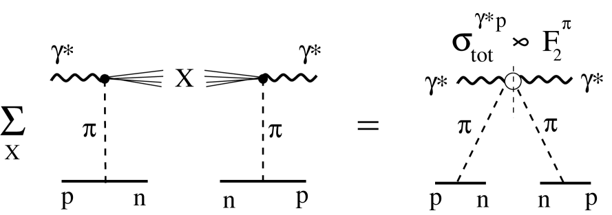
Figure 1: Graphical representation of the cross section of inclusive neutron production in hadron-proton collisions, in the fragmentation region of the proton.

Summing up all final states $X$ at a fixed invariant mass $M_{X}$ one arrives at the total hadron-pion cross section at c.m. energy $M_{X}$. This cross section is a slowly varying function of $M_{X}$, what leads to an approximate Feynman scaling. The rapidity gap covered by the pion exchange correspond to the energy, which is much smaller than the total c.m. collision energy squared

$${s^{\prime}\over s_{0}}={s\over M_{X}^{2}}\approx{1\over 1-z}\,,$$ (1)

where $s_{0}$ is the scale factor, usually fixed at $1\,\mbox{GeV}^{2}$; and $z=p_{n}^{+}/p_{p}^{+}$ is the fraction of the proton light-cone momentum carried by the neutron. If $z$ is large, it is close to Feynman $x_{F}$.

The pion exchange brings in the cross section the factor $(1-z)^{-2\alpha_{\pi}(t)}$, where $\alpha_{\pi}(t)$ is the pion Regge trajectory. This factor is independent of the collision energy, if $z$ is fixed, so the pion exchange contribution does not vanish with energy. The smaller is the 4-momentum transfer squared $t$, the closer one approaches the pion pole in the dispersion relation, and the more important is the pion contribution. However, the smallest values of $t$ are reached in the forward direction at $z\to 1$. The latter condition leads to the dominance of other Reggeons which have higher intercepts. Indeed, the corresponding Regge factor $(1-z)^{-2\alpha_{\footnotesize{I\!\!R}}(t)}$ for $\rho$ and $a_{2}$ Reggeons is about $1/(1-z)$ times larger than the one for pion. Although in general these Reggeons are suppressed by an order of magnitude compared to the pion k2p , they become important at $z\mathrel{\hbox to0.0pt{\lower 4.0pt\hbox{\hskip 1.0pt$\sim$}\hss}\raise 1.0pt\hbox{$>$}}0.9$.

The effective contribution of the axial-vector states ($a_{1}$ pole and $\rho$-$\pi$ cut) with the parameters fixed from phenomenology, was found recently kpss-spin to be crucial explaining data on azimuthal asymmetry of leading neutrons produced in $pp$ collisions. This Reggeon having a low intercept, affects the cross section at small $z$.

The most important correction, which is the main focus of this paper, is the effect of absorption, or initial/final state interactions. The active projectile partons participating in the reaction, as well as the spectator ones, can interact inelastically with the proton target or with the recoil neutron, and initiate particle production, which usually leads to a substantial reduction of the fractional neutron momentum. The probability that this does not happen, called sometimes survival probability of a large rapidity gap, leads to a suppression of leading neutrons produced at large $z$, because this process is associated with formation of a rapidity gap $\Delta y\sim-\ln(1-z)$. Some calculations predict quite a mild effect, of about $10\%$ even in the soft process $pp\to nX$ boreskov1 ; boreskov2 ; 3n ; ap , while others strong2 ; kkmr ; kmr ; kpss expect a strong reduction by about a factor of 2. See kkmr for a discussion of the current controversies in data and theory, for leading neutron production.

Notice that usually the absorptive corrections are calculated in a probabilistic way, convolving the gap survival probability with the cross section. We found, however, that the spin amplitudes of neutron production acquire quite different suppression factors kpss ; kpss-spin , and one should work with amplitudes, rather than with probabilities.

At first glance the absorptive corrections of the hadronic fluctuations of a highly virtual photon should be vanishingly small. However, the observed weak $Q^{2}$ dependence of nuclear shadowing in DIS demonstrates that this is not true: both shadowing and absorption are dominated by rare soft fluctuations of the photon interplay . This is why the absorptive corrections were calculated in ap relying on the effective absorption cross section adjusted to data on nuclear shadowing universal .

Even more simplified evaluation of absorptive corrections were performed in kkmr ; kmr , basing on the two component model for fluctuation of the virtual photon, soft and hard. The former was assumed to interact like the $\rho$ meson, while the latter cross section was fixed zero.

Below we perform explicit calculations of the absorptive corrections caused by the interactions of the fluctuations of a highly virtual photon within the dipole approach citezkl. Moreover, like in $pp$ collisions kpss , even a stronger absorption, related to the formation of a large color octet dipole in $\gamma^{*}\pi$ interaction, affects the large-$z$ part of the neutron spectrum. This effect has been missed in previous calculations of the absorption corrections.

Below our results are presented as follows. In Sect. II the spin structure of the amplitude without absorption corrections is presented, and the theoretical uncertainties in the evaluation of the cross section are discussed. Although the goal of the present paper is to study the possibilities of extraction of the pion structure function from data, we try to predict the cross section of leading neutron production, modeling the ratio of pion to proton structure functions.

Sect. III is devoted to the absorptive corrections, which are the main focus of this paper. The important observation is the production of a large size color octet dipole formed by the remnants of the virtual photon and pion. Initial/final state interaction of such a dipole, controlling the absorptive corrections at large $z$, only slightly depend on on the size of the $\bar{q}q$ fluctuation of the virtual photon, therefore almost no $Q^{2}$ is predicted. An examples of the absorption suppression factor $S_{4q}(b)$ and corrected for gluon radiation $\tilde{S}_{4q}(b)$ are shown in Fig. 4. The same figure demonstrates the reduced suppression factor $S_{\gamma^{*}}(b)$ at smaller $z$, where absorption of the hadronic fluctuations of the virtual photon plays major role. A sizable $Q^{2}$ dependence is predicted at smaller $z$, which is confirmed by data. The cross section of leading neutron production is found to be about twice smaller than the absorption uncorrected one, as is demonstrated in Fig. 7.

The isovector Reggeons, which also contribute to the neutron production, are evaluated in Sect. IV. The high-intercept $\rho$-Reggeon is important at large $z$ and large momentum transfer $q_{T}$ (it flips helicity). The low intercept $a_{1}$-Reggeon contributes at smaller $z$. The Regge $a_{1}$-pole itself is found to be very weak, and is replaced by an effective pole $\tilde{a}_{1}$, which also represents the $\rho$-$\pi$ Regge cut.

All the contributions together, corrected for absorption, reproduce data pretty well, as is demonstrated for the $q_{T}$- and $Q^{2}$-integrated cross sections in Fig. 8. The $Q^{2}$ and $q_{T}$ dependences are also well reproduced, as is shown in Fig. 9 and 10 respectively.

The possibility of extraction of the pion structure function from data is discussed in Sect. VI, and the sensitivity of the final results to the value of the pion-to-proton ratio of $F_{2}$ is demonstrated in Fig. 12.

II Born approximation

II.1 Measuring the pion structure function

In the Born approximation the pion exchange contribution to the amplitude of neutron production $\gamma^{*}p\to Xn$, depicted in Fig. 1, in the leading order in small parameter $m_{N}/\sqrt{s}$ has the form

$$A^{B}_{p\to n}(\vec{q},z)=\bar{\xi}_{n}\left[\sigma_{3}\,q_{L}+\frac{1}{\sqrt{z}}\,\vec{\sigma}\cdot\vec{q}_{T}\right]\xi_{p}\,\phi^{B}(q_{T},z)\,,$$ (2)

where $\vec{\sigma}$ are Pauli matrices; $\xi_{p,n}$ are the proton or neutron spinors; $\vec{q}_{T}$ is the transverse component of the momentum transfer;

$$q_{L}=\frac{1-z}{\sqrt{z}}\,m_{N}.$$ (3)

At small $1-z\ll 1$ the pseudoscalar amplitude $\phi^{B}(q_{T},z)$ has the triple-Regge form,

$$\phi^{B}(q_{T},z) = \frac{\alpha_{\pi}^{\prime}}{8}\,G_{\pi^{+}pn}(t)\,\eta_{\pi}(t)\,(1-z)^{-\alpha_{\pi}(t)}$$ (4)

$$\times A_{\gamma^{*}\pi^{\to}X}(M_{X}^{2})\,,$$

where $M_{X}^{2}=(1-z)s$, and the 4-momentum transfer squared $t$ has the form,

$$-t=q_{L}^{2}+{1\over z}\,q_{T}^{2}\,,$$ (5)

and $\eta_{\pi}(t)$ is the phase (signature) factor which can be expanded near the pion pole as,

$$\eta_{\pi}(t)=i-ctg\left[\frac{\pi\alpha_{\pi}(t)}{2}\right]\approx i+\frac{2}{\pi\alpha_{\pi}^{\prime}}\,\frac{1}{m_{\pi}^{2}-t}\,.$$ (6)

We assume a linear pion Regge trajectory $\alpha_{\pi}(t)=\alpha_{\pi}^{\prime}(t-m_{\pi}^{2})$ with $\alpha_{\pi}^{\prime}\approx 0.9\,\mbox{GeV}^{-2}$. The imaginary part in (6) is neglected in what follows, because its contribution near the pion pole is small.

The effective vertex function $G_{\pi^{+}pn}(t)=g_{\pi^{+}pn}\exp(R_{1}^{2}t)$, where $g^{2}_{\pi^{+}pn}(t)/8\pi=13.85$. The value of the slope parameter $R_{1}$ is specified below.

The amplitudes in (2)-(4) are normalized as,

$$\sigma^{\gamma^{*}\pi^{+}}_{tot}(s^{\prime}=M_{X}^{2})={1\over M_{X}^{2}}\sum\limits_{X}|A_{\gamma^{*}\pi^{+}\to X}(M_{X}^{2})|^{2}\,,$$ (7)

where different hadronic final states $X$ are summed at fixed invariant mass $M_{X}$. Correspondingly, the differential cross section of inclusive neutron production reads bishari ; 2klp ,

$$z\,\frac{d\sigma^{B}_{p\to n}}{dz\,dq_{T}^{2}} = \left(\frac{\alpha_{\pi}^{\prime}}{8}\right)^{2}|t|G_{\pi^{+}pn}^{2}(t)\left|\eta_{\pi}(t)\right|^{2}(1-z)^{1-2\alpha_{\pi}(t)}$$ (8)

$$\times \sigma^{\gamma^{*}\pi^{+}}_{tot}(s^{\prime}=M_{X}^{2})\,.$$

The virtual photoabsorption cross section can be expressed in terms of the structure function,

$$\sigma^{\gamma^{*}\pi^{+}}_{tot}(s^{\prime}=M_{X}^{2})=\frac{4\pi^{2}\alpha_{em}}{Q^{2}}\,F_{2}^{\pi}(x_{\pi},Q^{2}),$$ (9)

where

$$x_{\pi}=\frac{Q^{2}}{M_{X}^{2}}=\frac{x}{1-z},$$ (10)

and $x=Q^{2}/s$.

Thus, the process of leading neutron production in DIS described by Eq. (8), offers a unique opportunity to measure the pion structure function at small $x$.

Experimental data are usually presented in the form of ratio of neutron production and inclusive DIS cross sections zeus-2002 ; zeus-2007 , which in the Born approximation can be represented as

$$\frac{1}{\sigma_{inc}}\,\frac{d\sigma^{B}_{p\to n}}{dz\,dq_{T}^{2}}=\left(\frac{\alpha_{\pi}^{\prime}}{8}\right)^{2}|t|\,G_{\pi^{+}pn}^{2}(t)\left|\eta_{\pi}(t)\right|^{2}$$ (11)

$$\times \frac{(1-z)^{1-2\alpha_{\pi}(t)}}{z}\,R_{\pi/N}(x_{\pi},Q^{2})\,\frac{F_{2}^{p}(x_{\pi},Q^{2})}{F_{2}^{p}(x,Q^{2})}\,,$$

where

$$R_{\pi/N}(x_{\pi},Q^{2})=\frac{F_{2}^{\pi}(x_{\pi},Q^{2})}{F_{2}^{p}(x_{\pi},Q^{2})}.$$ (12)

The last factor in the right-hand side of Eq. (11) is known and provides a sizable suppression. Indeed, at small $x<0.01$ the measured proton structure functions can be parametrized as

$$F_{2}^{p}(x,Q^{2})=c(Q^{2})\left({1\over x}\right)^{\lambda(Q^{2})},$$ (13)

where $\lambda(Q^{2})=a\,\ln(Q^{2}/\Lambda^{2})$ with $a=0.048$ and $\Lambda=0.29\,\mbox{GeV}$ h1-par . $F_{2}^{p}(x_{\pi},Q^{2})/F_{2}^{p}(x,Q^{2})$ acquires a considerable suppression factor $(1-z)^{\lambda(Q^{2})}$. For example, at $z=0.8$ and $Q^{2}=13\,\mbox{GeV}^{2}$ (the mean value in zeus-2007 ) this factor is $0.68$. This factor is the main source of $Q^{2}$ dependence of the fractional cross section (11), which turns out to be pretty weak. For further calculations we rely on the more realistic QCD fit mstw2008 .

II.2 What to expect?

The main unknown quantity in (11), which also is the main goal of experimental studies of this process, is the pion structure function, which enters the ratio (12). Here we attempt at specifying the expected value of the ratio $R_{\pi/N}(x_{\pi},Q^{2})$, Eq. (12).

The hadron structure function $F_{2}^{h}(x,Q^{2})$ is proportional to the total cross section of interaction of the virtual photon with the hadron, $F_{2}^{h}(x,Q^{2})=Q^{2}/(4\pi^{2}\alpha_{em})\,\sigma^{\gamma^{*}p}_{tot}(x,Q^{2})$. In the target rest frame interaction with a highly virtual photon is a perfect counter of the number of quarks in the target. Indeed, the interaction radius of a small ($\sim 1/Q^{2}$) dipole is also small ($\sim 1/\ln Q^{2}$), therefore interaction of the dipole simultaneously with two target valence quarks, separated by a large distance, is suppressed. So the small dipole interacts separately with each target quark via a colorless exchange (Pomeron), i.e. the dipole-quark cross section is finite and universal, and the total dipole-hadron cross section is proportional to the number of the quarks. One arrives at the additive quark model, which was first proposed, though ill justified, for soft hadronic interactions LF . However, a highly virtual photon interacting with a large light hadron this model should be rather accurate, so one should expect $R_{\pi/N}\equiv F_{2}^{\pi}/F_{2}^{p}=N_{q}^{\pi}/N_{q}^{p}$, where $N_{q}^{h}$ is the number of quarks in the hadron $h$.

One can also interpret this via the QCD evolution at small $x$. The cross section of interaction of a small-size $\bar{q}q$ dipole with a proton is proportional to gluon density fs ,

$$\sigma_{\bar{q}q}(r_{T},x)=\frac{\pi^{2}}{3}\alpha_{s}(Q^{2})\,xg(x,Q^{2})\,r_{T}^{2},$$ (14)

where $r_{T}\sim 1/Q$ is the transverse dipole separation. There are many experimental evidences for existence in the proton a semi-hard scale, the mean gluon transverse momentum, of an effective gluon mass, of the order of $Q_{0}\sim 700\,\mbox{MeV}$ kst2 ; spots1 ; spots2 . This means that gluons are located within a small distance $\sim r_{0}=0.3\,\mbox{fm}$ around the sources. Probing the proton at the semi-soft scale $Q_{0}$ one resolves only the ”constituent” quarks, but not their structure. At a higher scale the gluons and sea quarks are resolved as well, but the QCD evolution leaves them essentially within the same spots around the sources. Although the radius of the spots rises with $1/x$ as $\langle r^{2}\rangle=4\alpha^{\prime}\ln(1/x)$, the effective slope at a hard scale is small $\alpha^{\prime}\approx 0.1\,\mbox{GeV}^{-2}$ k3p ; spots2 ; data , and the spots in the proton do not overlap up to the energy of LHC k3p ; spots2 . Therefore, it is reasonable to expect that the amount of glue and sea quarks generated at small $x$ though the evolution, is proportional to the number of the quarks, which are resolved at the soft scale, and play role of the initial condition for the evolution.

II.2.1 3 valence quarks in the proton

In the non-relativistic quark model one may expect a simple relation,

$$R_{\pi/N}(x_{\pi},Q^{2})={2\over 3},$$ (15)

provided that $x$ is sufficiently small, and $Q^{2}$ is large. This value was used in all previous calculations of the cross section of leading neutron production in DIS.

It is clear, however, that the relation (15) is a simplification, which misses the possibility of interaction with those constituents of the proton, which are different from just three valence quarks. Indeed, even the process under consideration is an example: as is depicted in Fig. 1, the virtual photon probes quarks and antiquarks in the pion cloud of the proton.

II.2.2 A multiquark proton

A proton experiences quantum fluctuations to the states containing more than 3 quarks. This is pretty obvious at a hard scale, since the flavor-symmetric sea of quarks and antiquarks is generated perturbatively through the QCD evolution. Such a source of extra quarks ceases, at a soft scale, so one might think that the gluon density at small $x$ in the proton at the starting semi-hard scale is proportional to the number of valence quarks, like is assumed in Eq. (15).

There are, however, nonperturbative quantum fluctuations in the proton, which produce extra quarks at a soft scale, also contributing to the initial conditions for the evolution. One of such mechanisms is directly related to the process under consideration. Production of leading neutrons is a part of the inclusive DIS cross section and also contributes to $F_{2}^{p}$. On the other hand, as one can see in Fig. 1, the small dipole $\{\bar{q}q\}_{\gamma^{*}}$ does not interact with the 3-quark nucleons via gluonic exchanges, but interacts with the pion, i.e. with a pair of extra quarks in the proton. Within the pion cloud model of the proton the number of quarks in the denominator of the ratio Eq. (15) should be increased:

$$N_{q}^{p}\Rightarrow 3+2\langle n_{\pi}\rangle,$$ (16)

where $\langle n_{\pi}\rangle$ is the mean number of pions in the proton. The bottom bound for this correction is easy to estimate integrating the fractional cross section Eq. (12),

$$\frac{1}{\sigma_{inc}}\int\limits_{0}^{1}dz\int dq_{T}^{2}\,\frac{d\sigma^{B}_{p\to n}}{dz\,dq_{T}^{2}}=0.15.$$ (17)

Since neutral pion exchange should also provide a half of this contribution, we can estimate,

$$\langle n_{\pi}\rangle>0.225.$$ (18)

This is the bottom bound because other final states, like baryon resonances, should also be added. This estimate is compatible with evaluations in arm-bogdan , which ranges from $\langle n_{\pi}\rangle=0.25$ to $0.38$, dependent on the used model for the pion flux (uncorrected for absorption) and with earlier estimates in tony1 ; tony2 ; povh .

The mean number of pions can also be evaluated basing on the observed deviation from the Gottfried sum rule gottfried of the measured flavor asymmetry of the proton sea,

$$I_{AS}=\int\limits_{0}^{1}dx\left[\bar{d}_{p}(x)-\bar{u}_{p}(x)\right]$$ (19)

The E866 experiment at Fermilab measured the value of asymmetry at $I_{AS}=0.118\pm 0.012$ e866 , which results in the mean number of pions $\langle n_{\pi}\rangle=0.36$ jen-chieh , with the usual assumption that the weight of the $|\pi\Delta\rangle$ Fock state is half of that for the $|\pi N\rangle$ component. A somewhat larger values of flavor asymmetry, but with larger errors, were found in the NMC experiment, $I_{AS}=0.148\pm 0.039$ nmc , and HERMES, $I_{AS}=0.16\pm 0.03$ hermes , experiments. The deduced expectations for the number of pions are $\langle n_{\pi}\rangle=0.44$ and $0.48$ respectively.

The number of quarks in the proton gets contribution not only from the flavor asymmetric, like in Eq. (16), but also from the flavor symmetric sea. At importance of the latter indicate data e866 on $\bar{d}_{p}(x)/\bar{u}_{p}(x)$, which cannot be described by the pion cloud model tony2 ; jen-chieh , and need iso-scalar contributions, like $\sigma$ and $\omega$ mesons. The analysis of this data performed in sigma within the meson cloud model, conclude that data on $\bar{d}_{p}(x)/\bar{u}_{p}(x)$ ratio can be described with the weight factors $\langle n_{\sigma}\rangle=0.023-0.078$ and $\langle n_{\omega}\rangle=0.063-0.671$, which may be rather large, but are quite uncertain.

Inclusion of the flavor symmetric sea into the relation (16) might considerably increase the mean number of the proton constituents at the soft scale,

$$N_{q}^{p}=3+2\bigl{(}\langle n_{\pi}\rangle+\langle n_{\sigma}\rangle+\langle n_{\omega}\rangle\bigr{)}.$$ (20)

Although the contribution of the isoscalar mesons may be significant, its magnitude is model dependent and poorly known. Considering the above mentioned result of the E866 experiment, $\langle n_{\pi}\rangle=0.36$ as a lower value, we fix the total meson contribution at $\langle n_{meson}\rangle=0.5$ and and use it in the following calculations. With this value $N_{q}^{p}=4$ and instead of the simplified expectation Eq. (15), we will rely on

$$R_{\pi/N}(x_{\pi},Q^{2})={1\over 2},$$ (21)

Although this number has a large uncertainty, we will rely on it through all further calculations up to comparison with DIS data for neutron production. Eventually we will check the sensitivity of data to $R_{\pi/N}$.

Notice that we have not touched so far the nominator of this ratio, the number of quarks in the pion, $N_{\pi}$. Apparently, it might be also subject to corrections due to soft multiquark fluctuation, e.g. $\pi\to\pi\rho$, which is probably the strongest Fock component ($\pi\to 2\pi$ is forbidden). However, pion is the Goldstone meson with an abnormally small mass, so any fluctuation is strongly suppressed by the energy denominator. In particular, the amplitude of the $\pi\to\pi\rho$ transition is suppressed as $m_{\pi}^{2}/(m_{\rho}+m_{\pi})^{2}$. Therefore the weight factor for the $|\pi\rho\rangle$ Fock component is so small that can be safely neglected.

II.2.3 More uncertaities

Another theoretical uncertainty in Eq. (11) is related to the slope parameter $R_{1}^{2}$ of the pionic formfactor of the nucleon. It has to be fixed by phenomenology, but the results of model dependent analyses are quite diverse FMS ; R1-0 ; ponomarev ; kaidalov1 ; kaidalov2 and vary from zero to $R_{1}^{2}=2\,\mbox{GeV}^{-2}$. This uncertainty affects the magnitude of the fractional cross section Eq. (11), especially at medium values of $z$. The forward cross section $(1/\sigma_{inc})d\sigma^{B}/dzdq_{T}^{2}|_{q_{T}=0}$ calculated in the Born approximation Eq. (11) is depicted in Fig. 2 by the strip between upper ($R_{1}^{2}=0$) and bottom ($R_{1}^{2}=2\,\mbox{GeV}^{-2}$) curves. The calculations are done at $Q^{2}=14\,\mbox{GeV}^{2}$, which is the mean value for the DIS data zeus-2007 at $Q^{2}>2\,\mbox{GeV}^{2}$ also depicted Fig. 2.

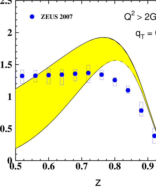
Figure 2: (Color online) The forward fractional cross section of neutron production in DIS calculated in the Born approximation, Eq. (11), with $R_{1}^{2}=0$ (upper curve) and $R_{1}^{2}=2\,\mbox{GeV}^{-2}$ (bottom curve). Data points are the results of the ZEUS experiment zeus-2007 .

As we mentioned above, the $Q^{2}$ dependence of the fractional cross section is quite weak.

We see that even within the uncertainty in the parameter $R_{1}$, the Born approximation significantly overestimates data zeus-2007 at large $z$, where the pion pole is expected to dominate. For further calculations we fix $R_{1}^{2}=0.3\,\mbox{GeV}^{-2}$, which was chosen in k2p ; kaidalov1 ; kaidalov2 ; kkmr ; kmr as most reliable.

III Absorptive corrections

Calculation of absorptive corrections, or initial/final state interactions, is quite complicated in momentum representation, where they require multi-loop integrations. However, these corrections factorize in impact parameters,

$$f_{p\to n}(b,z)=f^{B}_{p\to n}(b,z)\,S(b,z,s)\,,$$ (22)

where $S(b,z,s)$ is the suppression factor caused by absorption. Then one can Fourier transform the amplitude back to momentum representation, and the calculations are greatly simplified. So, we should first perform Fourier transformation of the amplitude Eq. (2) to impact parameter representation.

III.1 Impact parameter representation

The partial Born amplitude at impact parameter $\vec{b}$, corresponding to (2), has the form,

$$f^{B}_{p\to n}(\vec{b},z)=\bar{\xi}_{n}\left[\sigma_{3}\,q_{L}\,\theta^{B}_{0}(b,z)-i\,\frac{\vec{\sigma}\cdot\vec{b}}{\sqrt{z}\,b}\,\theta^{B}_{s}(b,z)\right]\xi_{p},$$ (23)

where

$$\theta^{B}_{0}(b,z) = \int d^{2}q_{T}\,e^{i\vec{b}\vec{q}_{T}}\,\phi^{B}(q_{T},z)$$ (24)

$$= \frac{N(z)}{1-\beta^{2}\epsilon^{2}}\,\left[K_{0}(\epsilon b)-K_{0}(b/\beta)\right]\,;$$

$$\theta^{B}_{s}(b,z) = {1\over b}\int d^{2}q_{T}\,e^{i\vec{b}\vec{q}_{T}}\,(\vec{b}\cdot\vec{q})\,\phi^{B}(q_{T},z)$$ (25)

$$= \frac{N(z)}{1-\beta^{2}\epsilon^{2}}\,\left[\epsilon\,K_{1}(\epsilon b)-\frac{1}{\beta}\,K_{1}(b/\beta)\right]\,.$$

Here

$$N(z)=\frac{1}{2}\,g_{\pi^{+}pn}\,z(1-z)^{\alpha^{\prime}_{\pi}(m_{\pi}^{2}+q_{L}^{2})}e^{-R_{1}^{2}q_{L}^{2}}A_{\gamma^{*}\pi\to X}(M_{X}^{2})$$ (26)

$$\epsilon^{2} = z(q_{L}^{2}+m_{\pi}^{2})\,,$$

$$\beta^{2} = {1\over z}\,\left[R_{1}^{2}-\alpha_{\pi}^{\prime}\,\ln(1-z)\right]\,.$$ (27)

To simplify the calculations we replaced here the Gaussian form factor, $\exp(-\beta^{2}q_{T}^{2})$, by the monopole form $1/(1+\beta^{2}q_{T}^{2})$, which is a good approximation at the small values of $q_{T}$ we are interested in (both shapes are ad hoc anyway). At the same time we retain the Gaussian dependence on $q_{L}$, which can be rather large.

III.2 Survival amplitude of a $\{\bar{q}q\}_{8}^{\gamma^{*}}$-$\{\bar{q}q\}_{8}^{\pi}$ dipole

At large $z\to 1$ the process under consideration is associated with the creation of a rapidity gap, $\Delta y=|\ln(1-z)|$, in which no particles are produced. Absorptive corrections, caused by initial and final state interactions of the projectile partons with the target and recoil neutron, may substantially reduce the probability of gap formation. Indeed, any inelastic interaction (color exchange) of the active or spectator partons should cause intensive multiparticle production filling the gap. Usually the corrected cross section is calculated probabilistically, i.e. convoluting the cross section with the survival probability factor (see kkmr and references therein). This recipe may work sometimes as an approximation, but only for $q_{T}$-integrated cross section. Otherwise one should rely on a survival amplitude, rather than probability. Besides, the absorptive corrections should be calculated differently for the spin-flip and non-flip amplitudes (see below).

The DIS on a virtual pion shown in Fig. 1, i.e. the inelastic collision $\gamma^{*}+\pi\to X$, can be seen as a color exchange between the colorless $\bar{q}q$ Fock component of the proton and the pion mediated by gluonic exchanges. Nonperturbatively, e.g. in the string model, the hadron collision looks like intersection and flip of strings. The final state of such a collision is two color octet $\bar{q}q$ pairs, originated from the photon and pion respectively, as is depicted in Fig. 3.

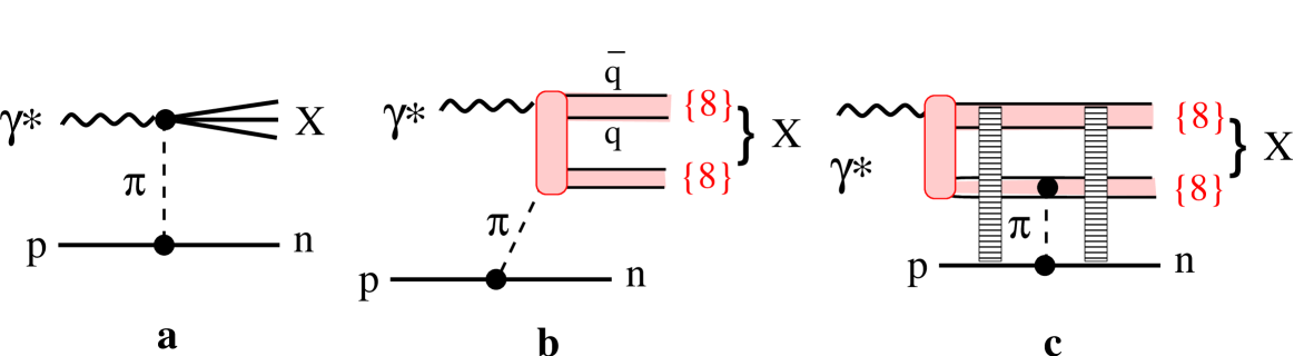
Figure 3: (Color online) a: Born graph with single pion exchange and excitation of the projectile photon, $\gamma^{*}+\pi\to X$; b: inelastic interaction, $\gamma^{*}+\pi\to X$, via color exchange, leading to the production of two color-octet $\bar{q}q$ dipoles which hadronize further to $X$; c: Fock state representation of the previous mechanism. A color octet-octet dipole as a 4-quark Fock component of the projectile photon, $\gamma^{*}\to\{\bar{q}q\}_{8}-\{\bar{q}q\}_{8}$, interacts with the target proton via $\pi^{+}$ exchange. This 4-quark state may experience initial and final state interaction via vacuum quantum number (Pomeron) exchange with the nucleons (ladder-like strips).

Hadronization of the color-octet dipole,$\{\bar{q}q\}_{8}-\{\bar{q}q\}_{8}$, leads to the production of different final states $X$.

According to Fig. 3b the produced color octet-octet state can experience final state interactions with the recoil neutron. On the other hand, at high energies multiple interactions become coherent, and one cannot specify at which point the color-exchange interaction happens, i.e. initial and final state interactions cannot be disentangled. In terms of the Fock state decomposition the projectile proton fluctuates into a 4-quark color octet-octet before the interaction with the target. The fluctuation life-time, or coherence time, rises with energy and at high energies considerably exceeds the longitudinal size of target proton (see, however, more detailed discussion below).

This leads to a different space-time picture of the process at high energies, namely: long in advance the interaction the incoming photon fluctuates into a 4-quark state $\gamma^{*}\to\{\bar{q}q\}_{8}$-$\{\bar{q}q\}_{8}$ which interacts with the target via pion exchange, as is illustrated in Fig. 3c. The survival probability amplitude $S_{4q}(\vec{b},\vec{r},s)$ for a dipole of separation $\vec{r}$ colliding with a nucleon at impact parameter $\vec{b}$ can be estimated on analogy with kpss as,

$$S_{4q}(\vec{b},\vec{r})=1-\,{\rm Im}\,f_{4q}(\vec{b},\vec{r})\approx\Bigl{[}1-\,{\rm Im}\,f_{\bar{q}q}(\vec{b},\vec{r})\Bigr{]}^{2}.$$ (28)

Here we rely on the large $N_{c}$ approximation and replaced a color octet-octet dipole by two triplet-antitriplet dipoles.

Notice that the mean $\{\bar{q}q\}_{8}^{\gamma^{*}}$-$\{\bar{q}q\}_{8}^{\pi}$ separation is large, and interaction of the $4q$-system with the nucleon target is soft, although the size of the $\{\bar{q}q\}_{8}^{\gamma^{*}}$ pair maybe as small as $1/Q$. Therefore, for the dipole amplitude $f_{\bar{q}q}(\vec{b},\vec{r},s)$ we employ the parametrization dependent on energy, rather than Bjorken $x$. The $b$-integrated phenomenological dipole cross section Eq. (32) is parametrized in the saturated form kst2 ,

$$\sigma_{\bar{q}q}(r,s)=\sigma_{0}(s)\left[1-e^{-r^{2}/R_{0}^{2}(s)}\right]\,,$$ (29)

where $R_{0}(s)=0.88\,\mbox{fm}\,(s_{0}/s)^{0.14}$; $s_{0}=1000\,GeV^{2}$;

$$\sigma_{0}(s)=\sigma^{\pi p}_{tot}(s)\left(1+\frac{3\,R^{2}_{0}(s)}{8\,\langle r^{2}_{ch}\rangle_{\pi}}\right)\,,$$ (30)

$\sigma^{\pi p}_{tot}(s)=23.6\,\mbox{mb}\times(s/s_{0})^{0.08}$, and the mean pion charge radius squared is $\langle r^{2}_{ch}\rangle_{\pi}=0.44\,\mbox{fm}^{2}$ r-pion .

The partial amplitude $f_{\bar{q}q}(\vec{b},\vec{r},s,\beta)$ of elastic scattering of a $\bar{q}q$ dipole with transverse separation $\vec{r}$ and fractional light-cone momenta $\beta$ (for $q$) and $1-\beta$ (for $\bar{q}$) on a proton at impact parameter $\vec{b}$ was derived in amir1 ; kpss ; amir2 ,

$$\,{\rm Im}\,f_{\bar{q}q}(\vec{b},\vec{r},s,\beta) = \frac{\sigma_{0}(s)}{8\pi B(s)}\,\Biggl{\{}\exp\left[-\frac{(\vec{b}-\vec{r}\beta)^{2}}{2B(s)}\right]+\exp\left[-\frac{[\vec{b}+\vec{r}(1-\beta)]^{2}}{2B(s)}\right]$$ (31)

$$- 2\exp\Biggl{[}-\frac{r^{2}}{R_{0}^{2}(s)}-\frac{[\vec{b}+(1/2-\beta)\vec{r}]^{2}}{2B(s)}\Biggr{]}\Biggr{\}}.$$

This partial amplitude satisfies the condition,

$$2\int d^{2}b\,{\,{\rm Im}\,}f_{\bar{q}q}(\vec{b},\vec{r},s,\beta)=\sigma_{\bar{q}q}(r,s),$$ (32)

The fractions $\beta$ and $1-\beta$ of the light-cone momentum of the $4q$-system carries by the color octets $\{\bar{q}q\}_{8}^{\gamma^{*}}$ and $\{\bar{q}q\}_{8}^{\pi}$, which are the debris of of the photon and pion respectively, are related to $z=1-M_{X}^{2}/s$ as,

$$\beta=\frac{Q^{2}+\langle m_{T}^{2}\rangle}{s(1-z)}\,,$$ (33)

where $m_{T}$ is the transverse mass of the pion debris $\{\bar{q}q\}_{8}^{\pi}$, which we fix at $\langle m_{T}^{2}\rangle=1\,\mbox{GeV}^{2}$.

The amplitude Eq. (31) also correctly reproduces the elastic $\pi$-$p$ slope $B^{\pi p}_{el}(s)$ provided that the effective slope parameter $B(s)$ has the form kpss ,

$$B(s)=B^{\pi p}_{el}(s)-{1\over 3}\,\langle r_{ch}^{2}\rangle_{\pi}-{1\over 8}\,R_{0}^{2}(s).$$ (34)

We use the Regge parametrization $B^{\pi p}_{el}(s)=B_{0}+2\alpha_{I\!\!P}^{\prime}\ln(s/\mu^{2})$, with $B_{0}=6\,\mbox{GeV}^{-2}$, $\alpha_{I\!\!P}^{\prime}=0.25\,\mbox{GeV}^{-2}$, and $\mu^{2}=1\,\mbox{GeV}^{2}$.

To get the differential cross section the absorption corrected Born amplitude of neutron production, $f_{p\to n}(\vec{b},\vec{r},z)=f^{B}_{p\to n}(\vec{b},z)\,S_{4q}(\vec{b},\vec{r},z,s)$, should be Fourier transferred back to the momentum representation, squared and averaged over the dipole size $r$,

$$z\,\frac{d\sigma_{p\to n}}{dz\,dq_{T}^{2}}=\left|f_{p\to n}(q_{T},z)\right|^{2}=\frac{1}{(2\pi)^{4}}\int d^{2}r\,W^{2}(r,M_{X}^{2})$$ (35)

$$\times \int d^{2}b\,d^{2}b^{\prime}\,e^{i\vec{q}_{T}(\vec{b}-\vec{b}^{\prime})}f_{p\to n}^{\dagger}(\vec{b},\vec{r},z)f_{p\to n}(\vec{b}^{\prime},\vec{r},z),$$

where $W^{2}(r,M_{X})$ is the probability distribution of impact parameter of $\gamma^{*}\pi$ collision at c.m. energy $M_{X}$. To simplify numerical calculation we employ here the same approximation as in kpss assuming that each amplitude can be averaged over $r$ separately, i.e. the absorption factor $S_{4q}(b,z,s)$ in (22) is related to one in (28) as

$$\bigl{\langle}S_{4q}(\vec{b},\vec{r},z,s)\bigr{\rangle}_{r}=\int d^{2}r\,W(r,Q^{2},M_{X}^{2})\,S_{4q}(\vec{b},\vec{r},z,s).$$ (36)

To proceed further we have to specify the distribution $W(r,M_{X}^{2})$ over the size $r$ of the $\{\bar{q}q\}_{8}^{\gamma^{*}}$-$\{\bar{q}q\}_{8}^{\pi}$ dipole, which is the impact parameter of the $\gamma^{*}\pi$ collision at c.m. energy $M_{X}$. Therefore, the $r$-distribution $W(r,M_{X}^{2})$ is given by the partial elastic photon-pion amplitude $f_{el}^{\gamma^{*}\pi}(r,M_{X}^{2})$, for which we use the normalized Gaussian $r$-dependence,

$$W(r,Q^{2},M_{X}^{2})=\frac{\exp\left[-r^{2}/4B^{\gamma^{*}\pi}_{el}(Q^{2},M_{X}^{2})\right]}{4\pi\,B^{\gamma^{*}\pi}_{el}(Q^{2},M_{X}^{2})}.$$ (37)

With a good precision, checked numerically $\bigl{\langle}S_{4q}(\vec{b},\vec{r},z,s)\bigr{\rangle}_{r}\approx\bigl{\langle}1-\,{\rm Im}\,f_{\bar{q}q}(\vec{b},\vec{r},z,s)\bigr{\rangle}_{r}^{2}$, where

$$\bigl{\langle}\,{\rm Im}\,f_{\bar{q}q}(\vec{b},\vec{r},z,s)\bigr{\rangle}_{r} = \frac{\sigma_{0}(s)}{8\pi}\Biggl{\{}\frac{1}{{\cal B}_{\beta}(s,z)}\exp\left[-\frac{b^{2}}{2{\cal B}_{\beta}(s,z)}\right]+\frac{1}{{\cal B}_{1-\beta}(s,z)}\exp\left[-\frac{b^{2}}{2{\cal B}_{1-\beta}(s,z)}\right]$$ (38)

$$- \frac{2}{{\cal B}_{\xi}(s,z)\left[1+4B^{\gamma^{*}\pi}_{el}(M_{X}^{2})/R_{0}^{2}(s)\right]}\exp\left[-\frac{b^{2}}{2{\cal B}_{\xi}(s,z)}\right]\Biggr{\}}\,,$$

where

$${\cal B}_{\beta}(s,z)=B(s)+2\beta^{2}\,B^{\gamma^{*}\pi}_{el}(M_{X}^{2})\,,$$ (39)

$${\cal B}_{\xi}(z,s) = B(s)+2\xi^{2}\,B^{\gamma^{*}\pi}_{el}(M_{X}^{2});$$

$$\xi^{2} = \frac{(1/2-\beta)^{2}}{1+4B^{\gamma^{*}\pi}_{el}(M_{X}^{2})/R_{0}^{2}(s)}$$ (40)

The $Q^{2}$ and energy dependences of the elastic $\gamma^{*}\pi$ slope, $B^{\gamma^{*}\pi}_{el}(M_{X}^{2},Q^{2})$ are expected to be similar to what has been observed for electroproduction of different vector mesons, $\rho$, $\phi$, $J/\Psi$, in $\gamma^{*}p$ interactions rho-prod ; phi-prod ; psi-prod . It was found that the value of the slope saturates at $Q^{2}+m_{V}^{2}\gtrsim 5\,\mbox{GeV}^{2}$ at the universal level, $B_{el}^{\gamma^{*}p}=B_{0}^{\gamma^{*}p}+2\alpha^{\prime}_{{I\!\!P}}\ln(W^{2}/\mu^{2})$, with $B_{0}^{\gamma^{*}p}\approx 4\,\mbox{GeV}^{-2}$ and $\alpha^{\prime}_{{I\!\!P}}\approx 0.1\,\mbox{GeV}^{-2}$. Notice that the observed small value of the Pomeron trajectory slope is in a good accord with the theoretically expectation and is considerably smaller than $\alpha^{\prime}_{{I\!\!P}}\approx 0.25\,\mbox{GeV}^{-2}$ observed in soft processes, which are affected by saturation of unitarity k3p ; spots2 . For the $\gamma^{*}\pi$ slope at high $Q^{2}$ we use a similar form

$$B_{el}^{\gamma^{*}\pi}(M_{X}^{2},Q^{2})=B_{0}^{\gamma^{*}\pi}+2\alpha^{\prime}_{{I\!\!P}}\ln(M_{X}^{2}/\mu^{2}),$$ (41)

with $B_{0}^{\gamma^{*}\pi}\approx B_{0}^{\gamma^{*}p}-2\,\mbox{GeV}^{-2}$. The latter relation is is written in analogy to the systematics of slopes observed in soft hadronic collisions.

The result of numerical calculation of $S_{4q}(b,z)$ at $\sqrt{s}=100\,\mbox{GeV}$, $z=0.7$ and $Q^{2}=13\,\mbox{GeV}^{2}$ are shown as function of $b$ in Fig. 4 by the upper solid curve. The suppression factor hardly varies with $z$ and is slightly enhanced with energy.

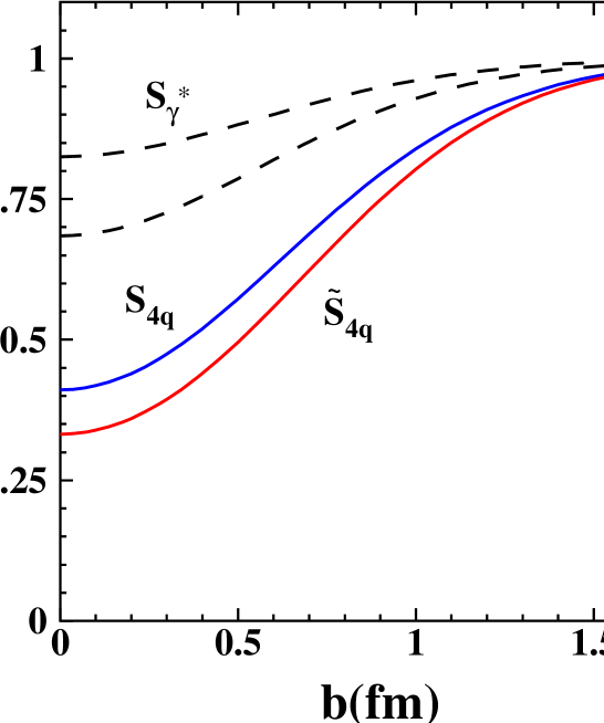
Figure 4: (Color online) Partial survival amplitudes $S_{4q}(b)$ (upper solid curve) calculated with Eq. (36) and $\tilde{S}_{4q}(b)$ (bottom curve) calculated with Eq, (44), at c.m. energy of $\gamma^{*}$-proton collision $\sqrt{s}=100\,\mbox{GeV}$ and $z=0.7$. Dashed curves show the suppression factor $S_{\gamma^{*}}(b)$ calculated for virtual photons with $Q^{2}=3$ (bottom) and $40\,\mbox{GeV}^{2}$ (upper dashed curve).

Naturally, the absorption effect is strongest for central collisions (suppression down to $40\%$), and gradually ceases towards the periphery.

III.3 Corrections for gluon radiation

So far our consideration was restricted to the lowest 4-quark Fock state of the photon, $\{\bar{q}q\}_{\gamma^{*}}-\{\bar{q}q\}_{\pi}$, contributing to neutron production. In the triple-Regge graph shown in Fig. 5 (left) this Fock state would correspond to the Pomeron gluonic latter without rungs, i.e. without gluon radiation.

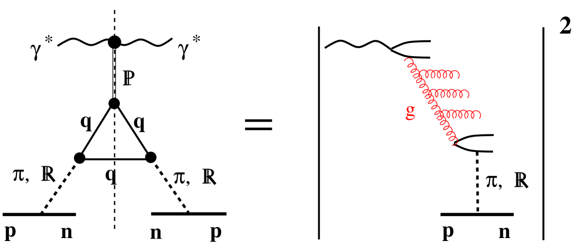
Figure 5: (Color online) Left: triple-Regge graph $\pi\pi{I\!\!P}$ for leading neutron production in DIS; Right: the unitarity cut of the of this graph, shown as a gluon comb.

Gluon bremsstrahlung, is however an important process, which is responsible for the observed rise of the cross sections with energy. So higher Fock states, like one depicted in Fig. 5 (right), containing gluons should be taken into account. Apparently they should lead to enhanced absorption effects.

In large-$N_{c}$ approximation a Fock component containing gluons can be replaced by a multi-dipole state mueller . The Pomeron is known to have a two-sheet topology (cylinder), which corresponds to the replacement of the 4-quark state by two $\bar{q}q$ dipoles as was done above. Every gluon radiated within one of the two Pomeron sheets creates an extra color triplet $\bar{3}3$ dipole. Correspondingly, the absorption factor gains an extra suppression factor $1-\,{\rm Im}\,f_{\bar{q}q}(r_{0})$. Thus, a Fock state containing besides 4-quark $n$ gluons provide a modified absorption factor $\tilde{S}_{4q}^{(n)}$,

$$S_{4q}(b)\Rightarrow\tilde{S}_{4q}^{(n_{g})}(b)=S_{4q}\,\left[1-\bigl{\langle}f_{\bar{q}q}(\vec{b},\vec{r}_{gg})\bigr{\rangle}_{r_{gg}}\right]^{n_{g}}.$$ (42)

Such states containing gluons, are characterized by two different scales, two typical dimensions spots1 ; spots2 . One is the large size of the pion, $\sim 1/\Lambda_{QCD}$, which dictates the mean size of the 4-quark color octet-octet dipole in (37). Another, much smaller distance is the mean size of a glue-glue dipole. Analysis of data on large-mass diffraction kst2 , as well as many other experimental observables spots2 show that this distance is quite small, $\langle r_{gg}\rangle\equiv r_{0}=0.3\,\mbox{fm}$. Thus, averaging of the dipole amplitude, which has the same size $r_{gg}$ as the glue-glue dipole, should be averaged as,

$$\bigl{\langle}f_{\bar{q}q}(\vec{b},\vec{r}_{gg})\bigr{\rangle}=\frac{1}{\pi r_{0}^{2}}\int d^{2}r_{gg}\,e^{-r_{gg}^{2}/r_{0}^{2}}\,f_{\bar{q}q}(\vec{b},\vec{r}_{gg})$$ (43)

Further, we assume that the number of radiated gluons has the Poisson distribution, so we can sum up the absorption factors of the s=Fock states with different number of gluons,

$$\tilde{S}_{4q}(b) = S_{4q}(b)e^{-\langle n_{g}\rangle}\sum\limits_{n_{g}=0}\frac{\langle n_{g}\rangle^{n_{g}}}{n_{g}!}\left[1-\bigl{\langle}f_{\bar{q}q}(\vec{b},\vec{r}_{gg})\bigr{\rangle}\right]^{n_{g}}$$ (44)

$$= S_{4q}(b)e^{-\langle n_{g}\rangle\langle f_{\bar{q}q}(b)\rangle}.$$

The mean number of radiated gluons $\langle n_{g}\rangle$ can be estimated looking at the $x$-dependence of the DIS cross section. In the leading-log approximation integration over rapidity of each gluon results in a factor $\ln(1/x)$. Summing over gluon number one gets for the total $\gamma^{*}$-proton cross section,

$$\sigma_{tot}^{\gamma^{*}p}\propto\sum\limits_{n_{g}=0}\frac{\bigl{[}g\ln(1/x)\bigr{]}^{n_{g}}}{n_{g}!}=\left({1\over x}\right)^{g},$$ (45)

where $g$ includes the coupling and other factors acquired due to radiation of each gluon.

Thus, according to Eq. (13) the mean number of radiated gluon reads,

$$\langle n_{g}\rangle=\lambda(Q^{2})\ln(1/x_{\pi}),$$ (46)

where $\lambda(Q^{2})$ is defined in (13).

Now we are in a position to calculate the modifies absorption factor Eq. (44). The result is plotted by the bottom solid curve in Fig. 4 in comparison with the uncorrected survival amplitude $S_{4q}$. Although the modified suppression is stronger, as was anticipated, the difference is rathe small. This is a result of smallness of $r_{0}$.

III.4 Coherence lengths for the photon Fock states

We have assumed so far that all the Fock components of the photon considered above have the lifetime, or coherence length, much longer than the dimension of the target. This is certainly true for the simplest Fock state $\gamma^{*}\to\bar{q}q$, which has a long coherence time, called Ioffe time (see more accurate evaluation in krt-dis ),

$$l_{c}^{\bar{q}q}=\frac{1}{2xm_{N}},$$ (47)

where $x\sim 10^{-3}$ in the kinematics of HERA.

However for the 4-quark Fock states this is not obvious. The coherence length is given by

$$l_{c}^{4q}=\frac{1}{q_{L}}=\frac{\sqrt{z}}{(1-z)m_{N}}.$$ (48)

This coherence time becomes very long for large $z\to 1$

Since the target nucleon size is $r_{N}\sim 1\,\mbox{fm}$, only at $z\mathrel{\hbox to0.0pt{\lower 4.0pt\hbox{\hskip 1.0pt$\sim$}\hss}\raise 1.0pt\hbox{$>$}}0.8$ the coherence length Eq. (48) is sufficiently long to rely on the above evaluations of the absorptive effects.

In another limit of a very short coherence length $l^{4q}_{c}\ll r_{N}$ not only initial, but also final state interactions of the 4-quark state are impossible, because even the the interaction time and time scale of creation of this state exceed the nucleon size. In this case the absorptive corrections are generated only by the interaction of long-living $\bar{q}q$ fluctuations of the photon. In this case the absorption factor has the form,

$$S_{\gamma^{*}}(b)=1-\bigl{\langle}\,{\rm Im}\,f_{\bar{q}q}(\vec{b},\vec{r},\alpha)\bigr{\rangle}_{r,\alpha},$$ (49)

where the partial elastic amplitude $\,{\rm Im}\,f_{\bar{q}q}(\vec{b},\vec{r},\alpha)$ is given by Eq. (31). The averaging over the transverse dipole separation $\vec{r}$, and the fractional light-cone momentum of the quark, $\alpha$, is done as follows,

$$\bigl{\langle}\,{\rm Im}\,f_{\bar{q}q}(\vec{b},\vec{r},\alpha)\bigr{\rangle}_{r,\alpha}=\left[\int\limits_{0}^{1}d\alpha\int d^{2}r\sigma_{\bar{q}q}(r,x_{\pi})\,\left|\Psi_{\bar{q}q}(r,\alpha,Q^{2})\right|^{2}\right]^{-1}\int\limits_{0}^{1}d\alpha\int d^{2}r\sigma_{\bar{q}q}(r,x_{\pi})\left|\Psi_{\bar{q}q}(r,\alpha,Q^{2})\right|^{2}\,{\rm Im}\,f_{\bar{q}q}(\vec{b},\vec{r},\alpha),$$ (50)

where the weight factor $\left|\Psi_{\bar{q}q}\right|^{2}=\left|\Psi_{\bar{q}q}^{T}\right|^{2}+\left|\Psi_{\bar{q}q}^{L}\right|^{2}$ contains the standard photon distribution functions bjorken1 ; bjorken2 . Notice the importance of the factor $\sigma_{\bar{q}q}(r,x_{\pi})$, which comes from the Born amplitude of neutron production. Without this factor the result of (50) would be zero krt-dis , because the normalization of the distribution function of transversely polarized photons, $\Psi_{\bar{q}q}^{T}$ is ultraviolet divergent. This divergency corresponds to ultra-heavy $\bar{q}q$ fluctuations, which dominate in a transversely polarized photon in vacuum. However, such fluctuation are ”sterile”, i.e. cannot interact (color transparency), while the process under consideration contains at least one dipole interaction.

Examples of the results for $S_{\gamma^{*}}(b)$ calculated at $Q^{2}=3$ and $40\,\mbox{GeV}^{2}$ are plotted in Fig. 4 by dashed curves. Apparently, the $Q^{2}$ dependence of the absorption factor is rather weak. This was anticipated, because in (50) we average the dipole amplitude squared, similar to diffraction of nuclear shadowing. The integral over $\alpha$ turns out to be dominated by the aligned-jet configurations aligned-jet , i.e. by the endpoint behavior of the distribution functions, $\alpha\mathrel{\hbox to0.0pt{\lower 4.0pt\hbox{\hskip 1.0pt$\sim$}\hss}\raise 1.0pt\hbox{$<$}}m_{q}^{2}/Q^{2}$ k-povh . The corresponding $\bar{q}q$ transverse separation becomes rather large, $\sim 1/m_{q}$, and independent of $Q^{2}$, $\langle r^{2}\rangle\sim Q^{2}\alpha(1-\alpha)+m_{q}^{2}$. We fixed the effective quark mass, which is in fact the infrared cutoff, at $m_{q}=0.15\,\mbox{GeV}$ adjusted to data on nuclear shadowing krt-dis .

Thus, we know the absorption corrections in two limiting regimes: (i) $l_{c}^{4q}\gg r_{N}$, in this case the suppression factor $\tilde{S}_{4q}(b)$ is given by Eq. (44) and depicted by solid curves in Fig. 4; (ii) $l_{c}^{4q}\ll r_{N}$, in this case the absorption factor $S_{\gamma^{*}}(b)$ is given by Eq. (49) and is shown by solid curves in Fig. 4. In order to interpolate between these limiting regimes we employ the following simple procedure,

$$S(b)=\tilde{S}_{4q}(b)\,F_{N}(q_{L})+S_{\gamma^{*}}(b)\bigl{[}1-F_{N}(q_{L})\bigr{]},$$ (51)

where the transition formfactor is chosen in the dipole form, $F_{N}(q_{L})=\bigl{(}1+q_{L}^{2}L^{2}\bigr{)}^{-1}=\left[1+\bigl{(}L/l_{c}^{4q}\bigr{)}^{2}\right]^{-1}$. The parameter $L$ characterizes the dimension of the target nucleon, so it should be of the order of $1\,\mbox{fm}$, and we fix it at this value, $L=1\,\mbox{fm}$, for further calculations. However, this parameter can be varied within a reasonable range. The $z$-dependence of the suppression factor Eq. (51) is plotted in Fig. 6 for few values of $b$.

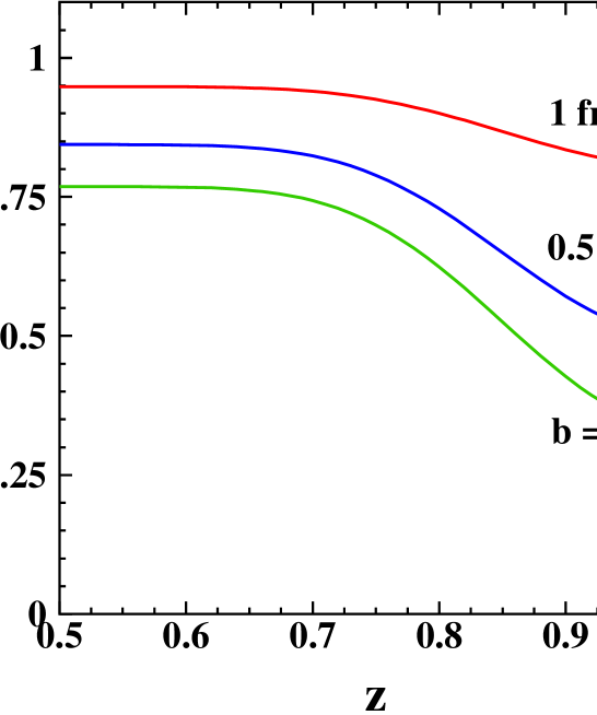
Figure 6: (Color online) The absorption factor $S(b,z)$, Eq. (51) as function of $z$ at fixed impact parameters $b=0,\ 0.5$ and $1\,\mbox{fm}$.

Notice that although the recipe Eq. (51) is partially ad hoc, it interpolates between the two known limiting regimes of very long, $l_{c}^{4q}\gg r_{N}$ ($z\gtrsim 0.8$), and very short, $l_{c}^{4q}\ll r_{N}$ ($z\sim 0.5$) coherence length. As far as these two regimes are predicted, the interpolation procedure should not affect the results significantly.

III.5 Cross section corrected for absorption

As soon as the absorption factor Eq. (51) is known, we can perform the inverse Fourier transformation to momentum representation,

$$f_{p\to n}(q_{T},z) = \frac{1}{(2\pi)^{2}}\int d^{2}b\,e^{i\vec{q}_{T}\cdot\vec{b}}$$

$$\times f^{B}_{p\to n}(\vec{b},z)\,S(b,z,Q^{2},s)$$

where the Born amplitude in impact parameters, $f^{B}_{p\to n}(\vec{b},z)$ is given by (23). So the absorption corrected partial spin amplitudes read,

$$\theta_{0,s}(b,z)=\theta^{B}_{0,s}(b,z)\,S(b,z).$$ (53)

Then the Fourier transformed amplitude reads,

$$A_{p\to n}(\vec{q}_{T},z)=\bar{\xi}_{n}\left[\sigma_{3}q_{L}\,\phi_{0}(q_{T},z)+\vec{\sigma}\vec{q}_{T}\frac{\phi_{s}(q_{T},z)}{\sqrt{z}}\right]\xi_{p},$$ (54)

where according to (24), (25) and (26),

$$\phi_{0}(q_{T},z) = \frac{N(z)}{2\pi(1-\beta^{2}\epsilon^{2})}\int\limits_{0}^{\infty}db\,b\,J_{0}(bq_{T})\,S(b,z)$$ (55)

$$\times \left[K_{0}(\epsilon b)-K_{0}\left({b\over\beta}\right)\right]\,;$$

$$q_{T}\,\phi_{s}(q_{T},z) = \frac{N(z)}{2\pi(1-\beta^{2}\epsilon^{2})}\int\limits_{0}^{\infty}db\,b\,J_{1}(bq_{T})\,S(b,z)$$ (56)

$$\times \left[\epsilon\,K_{1}(\epsilon b)-{1\over\beta}\,K_{1}\left({b\over\beta}\right)\right]\,.$$

Now we can calculate the differential cross section of inclusive production of neutrons corrected for absorption,

$$z\,\frac{d\sigma_{p\to n}}{dz\,dq_{T}^{2}}=\sigma_{0}(z,q_{T})+\sigma_{s}(z,q_{T})\,,$$ (57)

where

$$\sigma_{0}(z,q_{T}) = \frac{q_{L}^{2}}{s}\,\left|\phi_{0}(q_{T},z)\right|^{2}$$ (58)

$$\sigma_{s}(z,q_{T}) = \frac{q_{T}^{2}}{zs}\,\left|\phi_{s}(q_{T},z)\right|^{2}\,.$$ (59)

The effects of absorptive corrections are illustrated in Fig. 7

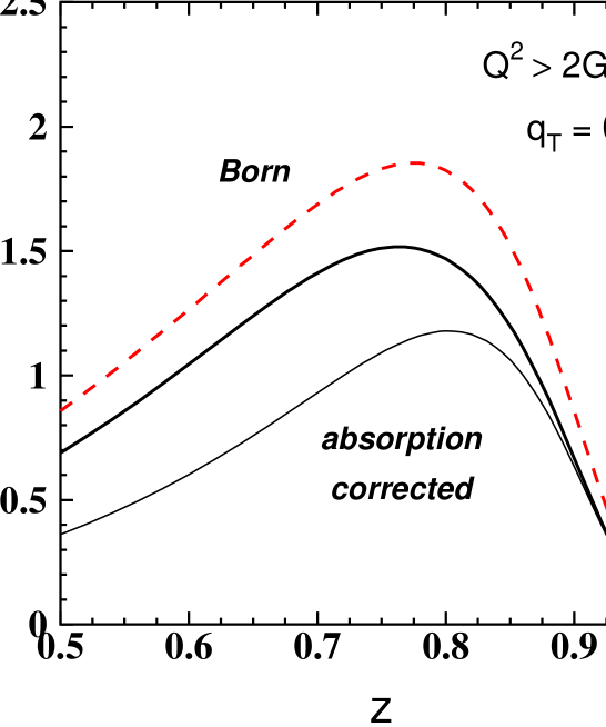
Figure 7: (Color online) Forward fractional cross section of neutron production in DIS calculated without absorption corrections (dashed curve); absorption suppressed by factor $\tilde{S}_{4q}(b)$ Eq. (44) (thin solid curve); and with the $z$-dependent absorption factor $S(b,z)$ Eq. (51) (thick solid curve).

The effect of suppression caused by the absorption factor $\tilde{S}_{4q}(b)$ defined in (58) is demonstrated by comparison of the fractional cross section of forward neutron production (dashed curve) with absorption suppressed result plotted by the thin solid curve. We observe a rather strong effect, absorption reduces the cross section by nearly factor 2. Inclusion of the coherence time effect results in a $z$-dependent absorption factor $S(b,z)$ defined in (51) and illustrated in Fig. 6. This final absorption corrected cross section is plotted in FIg. 7 by thick solid curve. We postpone comparison with data, because several more mechanisms of neutron production are to be added.

IV Other Reggeons

Besides pion exchange, other iso-vector Reggeons contribute to neutron production. Those are subdivided to natural parity Reggeons ($\rho,\ a_{2}$), which have high intercepts $\alpha_{R}(0)\approx 1/2$, and unnatural parity ones ($a_{1}$, $\pi^{\prime}$, etc.) with lower intercepts

IV.1 Natural parity Reggeons

The leading Reggeons contributing to neutron production are $\rho$ and $a_{2}$. At large invariant masses $M_{x}$ they do not interfere with the pion exchange and with each other. Indeed, summing over final states at fixed $M_{X}$ one gets the imaginary parts of the amplitudes for the processes, $\gamma^{*}+\pi\to\gamma^{*}+\rho$, or $\gamma^{*}+\rho\to\gamma^{*}+a_{2}$, which are suppressed by a power of $1/M_{X}$.

These amplitude are known to be dominated by their spin-flip part kane ; irving , so we neglect the non-flip term in what follows. In the Born approximation the leading Reggeons contribute to the cross section as,

$$\frac{1}{\sigma_{inc}}\left(\frac{d\sigma^{B}_{p\to n}}{dz\,dq_{T}^{2}}\right)_{\!\!R}=q_{T}^{2}\left(\frac{\alpha_{R}^{\prime}}{8}\right)^{2}\frac{(1-z)^{1-2\alpha_{R}(t)}}{z^{2}}\,$$ (60)

$$\times G_{R^{+}pn}^{2}(t)\left|\eta_{R}(t)\right|^{2}\frac{F_{2}^{R}(x_{\pi},Q^{2})}{F_{2}^{p}(x,Q^{2})}\,.$$

We consider two leading exchange degenerate Reggeons $\rho$ and $a_{2}$. The signature factor of the latter $\eta_{a_{2}}(t)=-i-\cot\left[{\pi\over 2}\alpha_{a_{2}}(t)\right]$ diverges at the so called nonsense wrong signature point, $t_{0}=-\alpha_{a_{2}}(0)/\alpha_{a_{2}}^{\prime}\approx-0.6\,\mbox{GeV}^{2}$. In order to kill this unphysical pole the residue function of the $a_{2}$ Reggeon must have a zero at this point, i.e. a factor $(1-t/t_{0})$. According to exchange degeneracy the residue function of the $\rho$-Reggeon should also contain this factor, which is not compensated by any pole at $t=t_{0}$. This is confirmed by data on differential cross section of reaction $\pi^{-}p\to\pi^{0}n$, which indeed has a dip at $t=t_{0}$ irving .

In this circumstances the $t$-dependences of $\rho$ and $a_{2}$ exchange amplitudes are rather uncertain. Since we are focused on small-$t$ region, the most reasonable solution seems to be to fix the signature factors of both Reggeons at $\eta_{R}(0)$. Moreover, basing on the exchange degeneracy of $\rho$ and $a_{2}$ Reggeons, we fix $\alpha_{\rho}(t)=\alpha_{a_{2}}(t)$ and $G_{\rho^{+}pn}(t)=G_{a_{2}^{+}pn}(t)$.

The contribution to the cross section of the spin-flip Reggeon amplitude can be described by the term similar to Eq. (59), properly modified,

$$\left(\frac{d\sigma_{p\to n}}{dz\,dq_{T}^{2}}\right)_{\!\!R}=\frac{2}{z}\sigma^{\rho}_{s}(z,q_{T})=\frac{2q_{T}^{2}}{z^{2}s}\left|\phi^{\rho}_{s}(q_{T},z)\right|^{2}\,,$$ (61)

where $\phi^{\rho}_{s}(q_{T},z)$, compared to Eq. (56), contains the imaginary part neglected for pions, and several modifications,

$$\phi^{\rho}_{s}(q_{T},z)=\frac{N_{\rho}(z)}{2\pi q_{T}\beta_{\rho}^{3}}\int\limits_{0}^{\infty}db\,b\,J_{1}(bq_{T})K_{1}(b/\beta_{\rho})S(b,z).$$ (62)

The further notations are,

$$N_{\rho}(z) = \frac{\pi\,\alpha_{\rho}^{\prime}}{4}\,g_{\rho^{+}pn}\,\eta_{\rho}(0)z(1-z)^{-\alpha_{\rho}(0)+\alpha^{\prime}_{\rho}\,q_{L}^{2}}$$ (63)

$$\times e^{-R_{\rho}^{2}q_{L}^{2}}A_{\gamma^{*}\rho\to X}(M_{X}^{2})$$

$$\beta_{\rho}^{2} = {1\over z}\,\left[R_{\rho}^{2}-\alpha_{\rho}^{\prime}\,\ln(1-z)\right]\,.$$ (64)

The absorptive corrections for the Reggeons are calculated with the same suppression factor $S(b)$ in (62). Its effect maybe somewhat stronger for Reggeons than for pions, since the interaction in this case is more central.

For the vertex function $G_{\rho NN}(t)=g_{\rho NN}\exp(R_{\rho}^{2}t)$ we rely on the phenomenological global Regge analysis irving of high-energy hadronic data, which results in $g_{\rho NN}=0.5\,g_{\pi NN}$, and $R^{2}_{\rho}=1\,\mbox{GeV}^{-2}$.

Notice that $N_{\rho}(z)$ contains an additional $z$-dependence, a factor $\sim 1/\sqrt{1-z}$, compared to the pion exchange, Eq. (26). This mean that at $z\to 1$ the $\rho/a_{2}$ Reggeon contribution should dominate over the pion exchange k2p , although at which $z$ this happens depends on the couplings strength.

IV.2 $a_{1}$-like exchanges

The study of spin effect in leading neutron production performed recently kpss-spin revealed important role of the axial-vector Reggeons, like $a_{1}$ meson. Interference of the related non-flip spin amplitude with spin-flip pion exchange well explained data on transverse single-spin asymmetry of leading neutrons produced in $pp$ collisions.

If fact, the situation with axial vector mesons is more complicated. Assuming vector meson dominance in the axial current, in analogy with the vector current, one arrives at a dramatic contradiction of the Adler relation for diffractive neutrino-production of pins with data, the effect called Piketti-Stodolsky puzzle pik-stod . It was proposed in marage that the source of the problem is the assumed axial-vector dominance, while in reality the $a_{1}$ pole is a very weak singularity, and the main contribution to the dispersion relation for the axial current comes from the $\rho$-$\pi$ cut. Indeed a detailed analysis of data on diffractive dissociation $\pi\to\rho\pi$ performed in kpss-spin shows that the invariant mass distribution of the produced in the $1^{+}S$ wave $\rho$-$\pi$ forms a pronounced narrow peak at a mass $M_{\tilde{a}_{1}}=1.12\,\mbox{GeV}$ close to the $a_{1}$ mass. In many instances one can tread such a $\rho$-$\pi$ Regge cut as an effective $\tilde{a}_{1}$-pole belkov ; marage ; pcac ; kpss-spin . Its contribution to the spin nin-flip part of the Born amplitude Eq. (2) reads,

$$\bigl{[}\phi^{\tilde{a}_{1}}_{0}(q_{T},z)\bigr{]}^{B} = \frac{\alpha_{\tilde{a}_{1}}^{\prime}}{8}\,G_{\tilde{a}_{1}pn}(t)\,\eta_{\tilde{a}_{1}}(t)(1-z)^{-\alpha_{\tilde{a}_{1}}(t)}$$ (65)

$$\times A_{\gamma^{*}\tilde{a}_{1}\to X}(M_{X}^{2})\,,$$

where

$$\eta_{\tilde{a}_{1}}(t)=-i-tg\!\left[\frac{\pi\alpha_{\tilde{a}_{1}}(t)}{2}\right].$$ (66)

The Regge trajectory of the $\rho$-$\pi$ cut has the form,

$$\alpha_{\tilde{a}_{1}}(t)=\alpha_{\pi\rho}(t)=\alpha_{\pi}(0)+\alpha_{\rho}(0)-1+\frac{\alpha_{\pi}^{\prime}\alpha_{\rho}^{\prime}}{\alpha_{\pi}^{\prime}+\alpha_{\rho}^{\prime}}\,t,$$ (67)

so $\alpha_{\tilde{a}_{1}}(0)=-0.5$; $\alpha_{\tilde{a}_{1}}^{\prime}=0.45\,\mbox{GeV}^{-2}$.

The $\tilde{a}_{1}NN$ vertex is parametrized as $G_{\tilde{a}_{1}pn}(t)=g_{\tilde{a}_{1}pn}\exp(R_{\tilde{a}_{1}}^{2}t)$. The ${\tilde{a}_{1}}NN$ coupling was evaluated in kpss-spin basing on PCAC and the second Weinberg sum rule, in which the spectral functions of the vector and axial currents are represented by the $\rho$ and the effective ${\tilde{a}_{1}}$ poles respectively. This leads to the following relations between the couplings,

$$\frac{g_{\tilde{a}_{1}NN}}{g_{\pi NN}}=\frac{m_{\tilde{a}_{1}}^{2}\,f_{\pi}}{2m_{N}\,f_{\rho}}\approx 0.5,$$ (68)

where $f_{\pi}=0.93m_{\pi}$ is the pion decay coupling; $f_{\rho}=\sqrt{2}m_{\rho}^{2}/\gamma_{\rho}$, and $\gamma_{\rho}$ is the universal coupling ($\rho NN$, $\rho\pi\pi$, etc), $\gamma_{\rho}^{2}/4\pi=2.4$.

Applying to the Born amplitude Eq. (65) the procedure of correcting for absorption, developed above, we Fourier transform the Born amplitude to impact parameters, introduce the absorption factor $S(b)$, the transform the result back to momentum representation and get,

$$\phi^{\tilde{a}_{1}}_{0}(q_{T},z)=\frac{N_{\tilde{a}_{1}}(z)}{2\pi\beta_{\tilde{a}_{1}}^{2}}\int\limits_{0}^{\infty}db\,b\,J_{0}(bq_{T})K_{0}(b/\beta_{\tilde{a}_{1}})S(b,z),$$ (69)

where

$$N_{\tilde{a}_{1}}(z) = \frac{\pi\,\alpha_{\tilde{a}_{1}}^{\prime}}{4}\,g_{{\tilde{a}_{1}}pn}\,\eta_{\tilde{a}_{1}}(0)z(1-z)^{-\alpha_{\tilde{a}_{1}}(0)+\alpha^{\prime}_{\tilde{a}_{1}}q_{L}^{2}}$$ (70)

$$\times e^{-R_{\tilde{a}_{1}}^{2}q_{L}^{2}}A_{\gamma^{*}{\tilde{a}_{1}}\to X}(M_{X}^{2})$$

$$\beta_{\tilde{a}_{1}}^{2} = {1\over z}\,\left[R_{\tilde{a}_{1}}^{2}-\alpha_{\tilde{a}_{1}}^{\prime}\,\ln(1-z)\right]\,.$$ (71)

For the sake of simplicity we assume that $A_{\gamma^{*}{\tilde{a}_{1}}\to X}(M_{X}^{2})$ is equal to the same amplitude on pion, $\rho$, or $a_{2}$ targets.

Besides, the interference between spin non-flip amplitudes with pion and $a$ exchanges also contributes. Altogether the corresponding part of the cross section reads,

$$\sigma_{0}(z,q_{T}) = \frac{q_{L}^{2}}{s}\,\Bigl{[}\left|\phi_{0}^{\pi}(q_{T},z)\right|^{2}+\xi^{2}\left|\phi_{0}^{\tilde{a}_{1}}(q_{T},z)\right|^{2}$$ (72)

$$+ 2\xi\,{\rm Re}\,\phi_{0}^{\pi{\tilde{a}_{1}}}(q_{T},z)\Bigr{]},$$

where $\xi=2m_{N}/\sqrt{|t|}\approx 2/(1-z)$ is a factor related to the spin structure of the axial-vector vertex kpss-spin .

In the interference term one needs to know the off-diagonal diffractive amplitude,

$$\sum\limits_{X}A_{\gamma^{*}{\tilde{a}_{1}}\to X}^{\dagger}A_{\gamma^{*}\pi\to X}=M_{X}^{2}\,\,{\rm Im}\,A_{\gamma^{*}\pi\to\gamma^{*}{\tilde{a}_{1}}}(M_{X}^{2},p_{T}=0)$$ (73)

The amplitude of the process $\gamma^{*}\pi\to\gamma^{*}{\tilde{a}_{1}}$ can be related to the reaction $\pi p\to{\tilde{a}_{1}}p$ relying on Regge factorization, and dominance of the diffractive excitation $\pi\to\rho\pi$ (see above). The amplitude Eq. (73) is suppressed compared with $\gamma^{*}\pi$ elastic scattering by the factor $\Omega$ defined as,

$$\Omega^{2} \equiv \frac{d\sigma(\gamma^{*}\pi\to\gamma^{*}{\tilde{a}_{1}})/dp_{T}^{2}}{d\sigma(\gamma^{*}\pi\to\gamma^{*}\pi)/dp_{T}^{2}}\Bigr{|}_{p_{T}=0}$$ (74)

$$\approx \frac{d\sigma(\pi p\to\pi\rho p)/dp_{T}^{2}}{d\sigma(\pi p\to\pi p)/dp_{T}^{2}}\Bigr{|}_{p_{T}=0}.$$

According to kpss-spin $L$ is energy independent and can be evaluated at $M_{X}^{2}=150\,\mbox{GeV}^{2}$ where data for diffractive $\pi p$ interactions are available, $d\sigma(\pi p\to\tilde{a}_{1}p)/dp_{T}^{2}\bigr{|}_{p_{T}=0}=1.67\,\mbox{mb}/\!\,\mbox{GeV}^{2}$. Then,

$$\Omega=\frac{\sqrt{16\pi\times 1.67\,\mbox{mb}/\,\mbox{GeV}^{2}}}{\sigma^{\pi p}_{tot}}=0.29.$$ (75)

Thus, the third term in (72) can be presented as,

$$2\,{\rm Re}\,\phi_{0}^{\pi{\tilde{a}_{1}}}(q_{T},z) = -2\Omega\,\frac{\tan\left[\pi\alpha_{\tilde{a}_{1}}(-q_{L}^{2})/2\right]}{|\eta_{\tilde{a}_{1}}(0)|}\,$$ (76)

$$\times \sqrt{\left|\phi_{0}^{\pi}(q_{T},z)\right|^{2}\left|\phi_{0}^{\tilde{a}_{1}}(q_{T},z)\right|^{2}},$$

where $\alpha_{\tilde{a}_{1}}(t)$ is given by Eq. (67) and we neglected the small imaginary part of the pion signature function Eq. (6).

Notice that the contribution of the $\tilde{a}_{1}$ exchange to neutron production has been well tested. Analogous calculations kpss-spin of the imaginary part of the $\pi-{\tilde{a}_{1}}$ interference led to a very good agreement with data on azimuthal asymmetry of neutrons produced by polarized protons.

V Numerical results

V.1 $z$-dependence

Two experiments at HERA, ZEUS zeus-2002 ; zeus-2007 and H1 h1 have studied leading neutron production in DIS. Their results are available for comparison with the same kinematics, integrated over $q_{T}$ within a fixed polar angle, $q_{T}<z\times 0.69\,\mbox{GeV}$, and up to a fixed maximum, $q_{T}<0.2\,\mbox{GeV}$. These data are depicted by round points in Fig. 8 in the upper and bottom panels respectively.

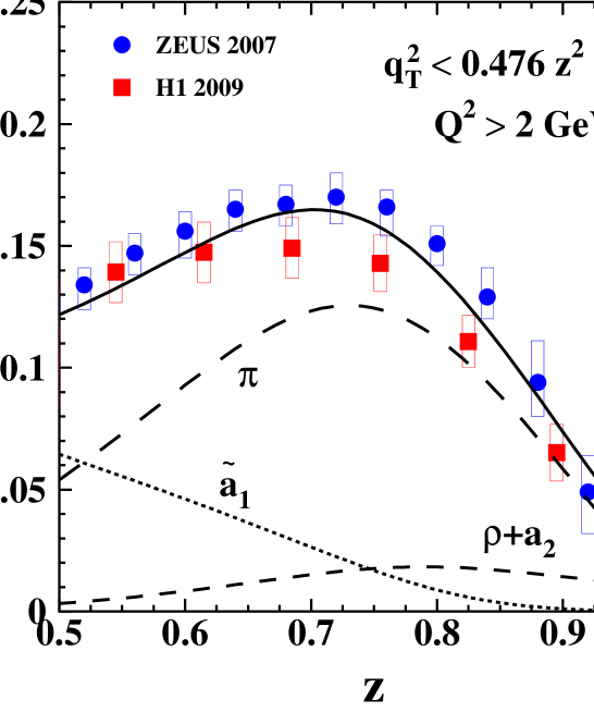
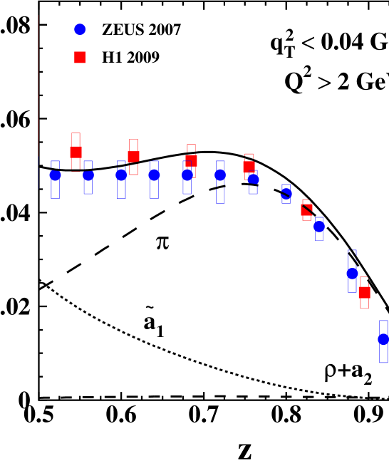
Figure 8: Fractional differential cross section of neutron production, integrated up to $q_{T}^{max}=0.2\,\mbox{GeV}$ (upper panel) and up to $q_{T}^{max}=z\times 0.69\,\mbox{GeV}$ (bottom panel). ZEUS data zeus-2007 are shown by round points. Data from the H1 experiment h1 depicted by squares are normalized as described in the text. In all sets of data the error are dominated by the systematic uncertainties. The pion pole contribution, calculated including absorptioncorrections is plotted by long-dashed curve (compare with Fig. 7). The contribution of $\rho$ and $a_{2}$ Reggeons and the effective $\tilde{a}_{1}$ pole are shown by short-dashed and dotted curves respectively. The sum of all these terms is presented by solid curve.

Analogous results of the H1 experiment are published in h1 , in the form of absolute values of the cross section. To compare with the ZEUS data and our calculations we normalized the H1 data dividing by inclusive DIS cross section $\sigma_{inc}=112\,{\rm pb}$ armen . The results are plotted in Fig. 8 by squares. Data for the fractional cross section of both experiments agree with each other if integrate in the large interval $q_{T}<z\times 0.69\,\mbox{GeV}$. However at small $q_{T}<0.2\,\mbox{GeV}$ the H1 cross section considerably exceeds the one measured by ZEUS at $z\lesssim 0.8$. This indicates at a significantly different $q_{T}$-slopes of the differential cross section measured in these two experiments.

The absorption corrected pion Regge pole contribution, which was shown by thick solid curve in Fig. 7, is depicted here by long-dashed curves. As was anticipated, the contribution of the effective $\tilde{a}_{1}$-Reggeon plotted by dotted curve, is vanishing at large $z$ because of the low Regge intercept. On the contrary, the $\rho$ and $a_{2}$ Reggeons are increasingly important towards large $z$, and even dominate at $z\to 1$.

V.2 $Q^{2}$-dependence

The full collections of ZEUS data named DIS with $Q^{2}>2\,\mbox{GeV}^{2}$ can be binned in order to trace the $Q^{2}$ dependence of the cross section. The result of such a binning is presented in Fig. 9.

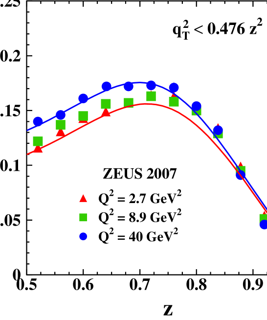
Figure 9: (Color online) $Q^{2}$ dependence of the fractional DIS cross section of neutron production, integrated up to $q_{T}^{max}=z\times 0.69\,\mbox{GeV}$. ZEUS data zeus-2007 for $Q^{2}=2.7,\ 8.9$ and $40\,\mbox{GeV}^{2}$ are shown by triangles, squares and round points respectively. The upper and bottom curves are calculated including all considered mechanisms at $Q^{2}=40$ and $2.7\,\mbox{GeV}^{2}$.

It demonstrate a clear increase of the fractional cross section with $Q^{2}$, especially at $z<0.8$. The variation with $Q^{2}$ of the calculated cross section originates solely from the absorption factor $S_{\gamma^{*}}$ (see Fig. 4) which is increasingly important towards small $z$ according to Eq. (51). This naturally explains the observed trend of a weakened $Q^{2}$ dependence at large $z$.

V.3 $q_{T}$-dependence

We also compare the $q_{T}$ dependence of the fractional differential cross section with few samples of ZEUS data presented in Fig. 10.

Figure 10: Fractional differential cross section of leading neutron production as function of neutron transverse momentum at several values of $z$ (solid curves). The contributions of pure pion exchange and of the iso-vector Reggeons, other than pion, are depicted by long and short-dashed curves respectively. ZEUS dara are plotted by round points. The large systematic errors (see zeus-2007 ) are not shown.

Our results are shown by solid curves, which sum up the pion (long-dashed curves) and Reggeon (short-dashed curves) contributions. Apparently, the role of Reggeons increases with $z$, especially at large $q_{T}$, where they significantly diminish the slope compared with the net pion contribution. Correspondingly, the calculated $q_{T}$ distribution acquires a bent shape, while the ZEUS data seem to prefer the Gaussian $q_{T}$-shape.

According to Eq. (5) at large $z$ and small $q_{T}$ one approaches the pion pole, $1/(t+m_{\pi}^{2})$. Therefore, the $q_{T}$-distribution of neutron production at large $z$ is expected to be rather steep, since is controlled by the small pion mass. However, the relative contribution of natural parity Reggeons rises, and eventually, they take over at $z\to 1$. Therefore, one could expect a sudden drop of the slope of the $q_{T}$-distribution.

Few examples of the $q_{T}$-dependence of the differential cross section plotted by solid curves, are compared with ZEUS data in Fig. 10. The contributions given by Eq. (57) and of Reggeons are plotted by long- and short-dashed curves respectively. Apparently, the Reggeons are important to achieve agreement with data.

Data of ZEUS are also presented in zeus-2007 as the slope of the $q_{T}$ distribution versus $z$, as is shown in Fig. 11.

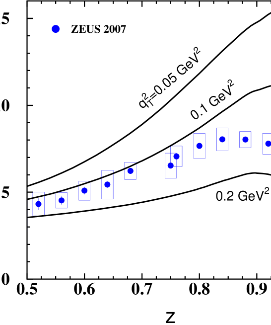
Figure 11: (Color online) ZEUS data zeus-2007 for the $q_{T}$-slope of the differential DIS cross section of leading neutron production as function of $z$. The solid curves present theoretical predictions calculated with Eq. (77) at fixed $q_{T}^{2}=0.5,\ 0.1$ and $0.2\,\mbox{GeV}^{2}$.

Theoretically, the slope is ill defined, if one does not specify in which interval of $q_{T}$ it was measured. The local slope, defined as

$$B(q_{T})=\frac{\partial}{\partial q_{T}^{2}}\,\ln\left[\frac{d\sigma_{p\to n}}{dzdq_{T}^{2}}\right],$$ (77)

apparently may vary with $q_{T}$. Although the results of the ZEUS experiment agree with $q_{T}$-independent slope (within large systematic errors), this is certainly not the case in the theory. For this reason we do not perform an explicit comparison of our results with data, but present in Fig. 11 the $z$-dependent slope $B(z,q_{T})$ calculated at few fixed values of $q_{T}^{2}=0.5,\ 0.1$ and $0.2\,\mbox{GeV}^{2}$. Remarkably, the results of calculations demonstrate flattening and a drop of $B(z,q_{T})$ towards $z=1$, similar to what is observed in data. Notice that these curves are not supposed to be directly compared with data, which cover an interval of $q_{T}$ dependent on $z$. The curves just show the uncertainty in the value of the slope, related to its ill definition.

VI Determining the pion structure function from data

Now we are in a position to try to answer the question, whether the process of leading neutron production in DIS can be consider as a tool to measure the pion structure function at small $x$. The answer depends on the sensitivity of the cross section to the number of quarks in the proton at a soft scale, and on the involved theoretical uncertainties.

If one trusted the way of calculations as is, then the number of quarks $N_{q}^{p}$ would affect only the ratio (12) and the cross section as a simple rescaling factor. However, the procedure of interpolation of the absorption factor, Eq. (51), between the known regimes of short and long coherence length, Eq. (48), leaves some freedom in adjusting the shape of the $z$-dependence of the fractional cross section. The parameter $L$ is known only by the order of magnitude, it should be comparable with the nucleon size, i.e. $L\sim 1\,\mbox{fm}$. So far we fixed it at this value, however, after rescaling the cross section assuming different number of quarks $N_{q}^{p}$, we can readjust this parameter within a reasonable range in order to achieve a better agreement with data.

We considered two additional scenarios, which look to us extreme, $N_{q}^{p}=3$ and $N_{q}^{p}=5$, which correspond to no mesons, or in average to one meson in the light-cone wave function of the proton at a soft scale, respectively. Correspondingly, we adjusted the length scale at $L=2\,\mbox{fm}$ and $L=0.5\,\mbox{fm}$ respectively. The results a shown in Fig. 12 in comparison with data.

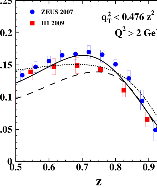
Figure 12: (Color online) Data are the same as in Fig. 8, upper panel. The dotted, solid and dashed curves are calculated with $N_{q}^{p}=3,\ 4,\ 5$, and with $L=2,\ 1$, and $0.5\,\mbox{fm}$, respectively.

Apparently, the solid curve does the best job describing the data, and being optimistic one may conclude that the version with $N_{q}^{p}=4$ is preferable. However, being skeptical one may say that the results of calculations are too model dependent to make a solid conclusion. Moreover, the relation between the ratio of pion to proton structure function and the mean number of quarks at a soft scale is based on the model of two scales in the proton spots2 , otherwise it may be broken.

VII Summary

To summarize, we highlight some of the results and observations.

• Production of leading neutrons with fractional momentum $z\to 1$ in DIS can serve as a way to measure the pion structure function at small $x$. However this method involves the several complications which are under investigation in this paper.

• We expect a reduction of the ratio $F_{2}^{\pi}(x)/F_{2}^{p}(x)$ compared with the usually assumed $2/3$. The deviation is due to the presence of a significant contribution of soft meson fluctuations in the proton wave function. While the contribution of the iso-vector mesons is constrained by the observed deviation from the Gottfried sum rule, the role of the iso-scalar mesons in the proton is less known. The calculations performed in this paper are done with the fixed ratio $F_{2}^{\pi}(x)/F_{2}^{p}(x)=1/2$.

• Even if the pion structure function is known, the fractional cross section of leading neutron production cannot be accurately predicted because of initial/final state interactions generating absorptive corrections, whose magnitude is under debate. Although the projectile particle in $\gamma^{*}p\to Xn$ is a highly virtual photon, we expect the effects of absorption at large $z$, to be nearly as strong, as in $pp\to Xn$. This happens due to formation of a strongly interacting color0octet dipole $\{\bar{q}q\}_{8}^{\gamma^{*}}$-$\{\bar{q}q\}_{8}^{\pi}$. The suppression factor $\tilde{S}_{4q}(b)$ depicted in Fig. 4 has a magnitude similar to $S_{5q}(b)$ in kpss ; kpss-spin .

• The coherence time Eq. (47), which is the lifetime of the strongly interacting projectile color-octet dipoles, is too short at medium values of $z$, and one should switch to the long-living $\bar{q}q$ fluctuations of the photon. The corresponding absorption factor $S_{\gamma^{*}}(b)$ is evaluated to be rather close to one, as is depicted in Fig. 4. The transition between the two regimes of absorption is illustrated in Fig. 6.

• Other iso-vector meson exchanges, heavier than pion, are also important. The meson-nucleon couplings of natural parity $\rho$ and $a_{2}$ Reggeons, which are predominantly spin-flip, were fixed by phenomenological Regge fits to high-energy hadronic data. The parameters of the unnatural parity $a_{1}$ Reggeon, which is non-spin-flip, are not well constrained by available data, and we fix them basing on the current algebra. Since the $a_{1}$ pole contribution was found to be very weak, we supplemented it by the $\rho$-$\pi$ cut, and treated them together as an effective $\tilde{a}_{1}$. Such an effective description was well tested in kpss-spin with the data on neutron azimuthal asymmetry. The two sets of Reggeons have quite different intercepts and affect the neutron production cross section in different regions of $z$. Fig. 8 shows that $\rho$ and $a_{2}$ are important at $z\to 1$, while $\tilde{a}_{1}$ is large at smaller $z$.

• Eventually, we additionally tested two extreme assumptions about the number of quarks in the proton at a soft scale, $N_{q}^{p}=3$ and $5$. In each case we readjusted the parameter $L$ in Eq. (51) within a reasonable range, however, could not reach a good agreement with data, as is demonstrated in Fig. 12.

Summarizing, our assumption Eq. (21) that the pion structure function at small $x$ is twice smaller than the proton one, is well supported by the parameter-free calculations of absorptive corrections and contribution of Reggeons, providing a good description of ZEUS and H1 data for leading neutron production in DIS, as function of $z$, $Q^{2}$ and $q_{T}$. Nevertheless, we should admit that the test is not really precise because of many theoretical and experimental uncertainties involved into the calculations.

- (1) B. Kopeliovich, B. Povh and I. Potashnikova, Z. Phys. C 73, 125 (1996) [arXiv:hep-ph/9601291].
- (2) B. Z. Kopeliovich, I. K. Potashnikova, I. Schmidt and J. Soffer, Phys. Rev. D 84, 114012 (2011)
- (3) K.G. Boreskov, A.A. Grigorian and A.B. Kaidalov, Sov. J. Nucl. Phys. 24, 411 (1976).
- (4) K.G. Boreskov, A.A. Grigorian, A.B. Kaidalov and I.I.Levintov, Sov. J. Nucl. Phys. 27, 813 (1978).
- (5) N. N. Nikolaev, W. Schafer, A. Szczurek and J. Speth, Phys. Rev. D 60, 014004 (1999) [arXiv:hep-ph/9812266].
- (6) U. D’Alesio and H. J. Pirner, Eur. Phys. J. A 7, 109 (2000) [arXiv:hep-ph/9806321].
- (7) V.A. Khoze, A.D. Martin and M.G. Ryskin, Eur. Phys. J. C18, 167 (2000).
- (8) A. B. Kaidalov, V. A. Khoze, A. D. Martin and M. G. Ryskin, Eur. Phys. J. C 47, 385 (2006).
- (9) V. A. Khoze, A. D. Martin and M. G. Ryskin, Eur. Phys. J. C 48, 797 (2006).
- (10) B. Z. Kopeliovich, I. K. Potashnikova, I. Schmidt and J. Soffer, Phys. Rev. D 78, 014031 (2008).
- (11) B. Kopeliovich and B. Povh, Z. Phys. A 356, 467 (1997).
- (12) B. Kopeliovich and B. Povh, Phys. Lett. B 367, 329 (1996).
- (13) B. Z. Kopeliovich, L. I. Lapidus and A. B. Zamolodchikov, JETP Lett. 33, 595 (1981) [Pisma Zh. Eksp. Teor. Fiz. 33, 612 (1981)].
- (14) M. Bishari, Phys. Lett. B 38, 510 (1972).
- (15) Yu. M. Kazarinov, B. Z. Kopeliovich, L. I. Lapidus and I. K. Potashnikova, Sov. Phys. JETP 43, 598 (1976) [Zh. Eksp. Teor. Fiz. 70, 1152 (1976)].
- (16) S. Chekanov et al. [ZEUS Collaboration], Nucl. Phys. B 637, 3 (2002).
- (17) S. Chekanov et al. [ZEUS Collaboration], Nucl. Phys. B 776, 1 (2007).
- (18) C. Adloff et al. [H1 Collaboration], Phys. Lett. B 520, 183 (2001).
- (19) A. D. Martin, W. J. Stirling, R. S. Thorne and G. Watt, Eur. Phys. J. C 63, 189 (2009); Eur. Phys. J. C 64, 653 (2009).
- (20) E. M. Levin and L. L. Frankfurt, JETP Lett. 2, 65 (1965).
- (21) B. Blättel, G. Baym, L. L. Frankfurt, H. Heiselberg and M. Strikman, Phys. Rev. D 47, 2761 (1993).
- (22) B. Z. Kopeliovich, A. Schäfer and A. V. Tarasov, Phys. Rev. D 62, 054022 (2000).
- (23) B. Z. Kopeliovich and B. Povh, J. Phys. G G 30, S999 (2004).
- (24) B. Z. Kopeliovich, I. K. Potashnikova, B. Povh and I. Schmidt, Phys. Rev. D 76, 094020 (2007).
- (25) B. Z. Kopeliovich, I. K. Potashnikova, B. Povh and E. Predazzi, Phys. Rev. Lett. 85, 507 (2000); Phys. Rev. D 63, 054001 (2001).
- (26) S. Chekanov et al. [ZEUS Collaboration], PMC Phys. A 1, 6 (2007) [arXiv:0708.1478 [hep-ex]].
- (27) A. Bunyatyan and B. Povh, Eur. Phys. J. A 27, 359 (2006)
- (28) A. W. Thomas, Phys. Lett. B 126, 97 (1983).
- (29) A. W. Schreiber, P. J. Mulders, A. I. Signal and A. W. Thomas, Phys. Rev. D 45, 3069 (1992).
- (30) S. Baumgärtner, H.J. Pirner, K. Königsmann and B. Povh, Z. Phys. A353, 397 (1996).
- (31) K. Gottfried, Phys. Rev. Lett. 18, 1174 (1967).
- (32) R. S. Towell et al. [FNAL E866/NuSea Collaboration], Phys. Rev. D 64, 052002 (2001).
- (33) G. T. Garvey and J. -C. Peng, Prog. Part. Nucl. Phys. 47, 203 (2001).
- (34) M. Arneodo et al. [New Muon Collaboration], Phys. Rev. D50, R1 (1994); Nucl. Phys. B 487, 3 (1997).
- (35) K. Ackerstaff et al. [HERMES Collaboration], Phys. Rev. Lett. 81, 5519 (1998).
- (36) F. Huang, R. -G. Xu and B. -Q. Ma, Phys. Lett. B 602, 67 (2004).
- (37) L. L. Frankfurt, L. Mankiewicz and M. I. Strikman, Z. Phys. A 334, 343 (1989).
- (38) G. Levman and K. Furutani, ZEUS note 92-107, 1992; preprint DESY 95-142, 1995.
- (39) L. A. Ponomarev, Sov. J. Part. Nucl. 7, 70 (1976) [Fiz. Elem. Chast. Atom. Yadra 7, 186 (1976)].
- (40) G.G. Arakelyan and K.G. Boreskov, Sov. J. Nucl. Phys. 30, 840 (1979); 31, 819 (1980).
- (41) G.G. Arakelyan, K.G. Boreskov and A.B. Kaidalov, Sov. J. Nucl. Phys. 33, 247 (1981).
- (42) S. Amendolia et al., Nucl. Phys. B277 (1986) 186.
- (43) B. Z. Kopeliovich, H. J. Pirner, A. H. Rezaeian and I. Schmidt, Phys. Rev. D 77, 034011 (2008).
- (44) B. Z. Kopeliovich, A. H. Rezaeian and I. Schmidt, Phys. Rev. D 78, 114009 (2008).
- (45) S. Chekanov et al. [ZEUS Collaboration], PMC Phys. A 1, 6 (2007).
- (46) S. Chekanov et al. [ZEUS Collaboration], Nucl. Phys. B 718, 3 (2005).
- (47) S. Chekanov et al. [ZEUS Collaboration], Nucl. Phys. B 695, 3 (2004).
- (48) A.H. Mueller, Nucl. Phys. B415, 373 (1994); it ibid B437, 107 (1995).
- (49) B. Z. Kopeliovich, J. Raufeisen and A. V. Tarasov, Phys. Rev. C 62, 035204 (2000).
- (50) J.M. Bjorken, J.B. Kogut and D.E. Soper, D 3, 1382 (1971).
- (51) J. D. Bjorken and J. Kogut, Phys. Rev. D8, 1341 (1973).
- (52) J. D. Bjorken, In *Lake Louise 1995, Quarks and colliders* 61-90, SLAC-PUB-95-6949; http://www.slac.stanford.edu/pubs/slacpubs/6750/slac-pub-6949.pdf
- (53) B. Kopeliovich and B. Povh, Z. Phys. A 356, 467 (1997).
- (54) H. E. Haber and G. L. Kane, Nucl. Phys. B 129, 429 (1977).
- (55) A. C. Irving and R. P. Worden, Phys. Rept. 34, 117 (1977).
- (56) C. A. Piketty and L. Stodolsky, Nucl. Phys. B 15, 571 (1970).
- (57) B. Z. Kopeliovich and P. Marage, Int. J. Mod. Phys. A 8, 1513 (1993).
- (58) A. A. Belkov and B. Z. Kopeliovich, Sov. J. Nucl. Phys. 46, 499 (1987) [Yad. Fiz. 46, 874 (1987)].
- (59) B. Z. Kopeliovich, I. K. Potashnikova, I. Schmidt and M. Siddikov, Phys. Rev. C 84, 024608 (2011).
- (60) F. D. Aaron et al. [H1 Collaboration], Eur. Phys. J. C 68, 381 (2010).
- (61) A. Bunyatyan, private communication.