The Minimum Variability Time Scale and its Relation to Pulse Profiles of Fermi GRBs

Abstract

We present a direct link between the minimum variability time scales extracted through a wavelet decomposition and the rise times of the shortest pulses extracted via fits of 34 Fermi GBM GRB light curves comprised of 379 pulses. Pulses used in this study were fitted with log-normal functions whereas the wavelet technique used employs a multiresolution analysis that does not rely on identifying distinct pulses. By applying a corrective filter to published data fitted with pulses we demonstrate agreement between these two independent techniques and offer a method for distinguishing signal from noise.

1 Introduction

One approach for probing light curves which has received attention (Nemiroff, 2000; Norris et al., 2005; Hakkila & Nemiroff, 2009; Nemiroff, 2012) is to express them as a series of displaced pulses, each with a parametric form. There is an appeal to this approach because fitting routines are well-understood and interpretations of rise time, decay time, full width at half max, etc, are possible. On the other hand, one must make certain assumptions when using the pulse-fitting procedure such as the choice of the functional form to use for an individual pulse and the number of parameters to be included in the fitting function. Moreover, light with high variability at low power may show variations which are not statistically significant.

A complementary approach using a wavelet-based analysis of a set of both long and short GRB light curves is discussed by MacLachlan et al. (2012) in which a time scale, $\tau_{\beta}$, is identified that marks the transition from white noise to a power law in the power density spectrum (a $f^{-\alpha}$ behavior). It is argued that over time scales smaller than $\tau_{\beta}$ the light curves appear stochastic and signal power is distributed uniformly. At time scales larger than $\tau_{\beta}$, identifiable structures (such as pulses) with signal power are no longer distributed uniformly over the periods of light variation. For this reason $\tau_{\beta}$ is referred to as the minimum variability time scale.

The analysis presented in (MacLachlan et al., 2012) is a non-parametric approach to probing light curves for time scales. It makes no assumptions about the nature of the structures in a given light curve that give rise to the $f^{-\alpha}$ character. The technique, however, offers no firm connection between $\tau_{\beta}$ and the constituent structures although it seems reasonable to associate $\tau_{\beta}$ with the scale of the smallest emitting structures present.

Results from an application of a log-normal pulse-fitting procedure to GRB light curves have been published by Bhat et al. (2012). In this paper we make a meta-analysis of the timing results presented by Bhat et al. (2012) compared with the techniques of MacLachlan et al. (2012) for a set of 34 GRBs used in both studies.

2 Analysis

We begin by considering the relation between $\tau_{\beta}$ and the pulse parameters given in Table 3 of Bhat et al. (2012). The parameters with temporal units in Table 3 are: time-since-trigger, rise time, decay time, and FWHM. In all, 34 GRBs comprising 379 pulses are considered here. We note that rise time, decay time, and FWHM as presented in Table 3 of Bhat et al. (2012) are tightly correlated and for the argument that follows are interchangeable without affecting the conclusions. However, we use rise time to make our argument because, as Bhat et al. (2012) noted, rise times are observed to be shorter than decay time and FWHM (see Table 3 in  Bhat et al. (2012)). We considered only those light curves from NaI detectors and summed over the energy acceptance as in Table 3 of Bhat et al. (2012) and in MacLachlan et al. (2012).

In Fig. 1 we plot the rise time for all 379 pulses (34 GRBs) along the vertical axis and $\tau_{\beta}$ along the horizontal. Note that for each GRB for which one $\tau_{\beta}$ is computed, there is a possibility for multiple pulses and therefore multiple rise times, hence the vertical columns of rise times for a single value of $\tau_{\beta}$. For a given column of pulse times the shortest pulse rise times are at the bottom and one finds larger rise times by moving up the column. An equality line is also shown which is the locus where $\tau_{\beta}$ equals rise time. Arguing as we do that $\tau_{\beta}$ represents the minimum variability time scale the space in the $\tau_{\beta}$-rise time plane below the equality line should be interpreted as a structureless white noise region. If some method were capable of discerning light curve structure in the region we define as white noise, then our assertion of having found a minimum variability time scale will have been disproven. Indeed, in Fig. 1 there are 27 pulses with rise times below the equality line. The uncertainties accompanying these 27 rise times are small, making their intrusion into the white noise region significant.

Table 1: Pulses with rise times smaller than $\tau_{\beta}$ but larger than bin widths. Pulse Number (#), rise (time), $\delta$rise (time), and bin width are taken from Table 3 of Bhat et al. (2012). The column labeled $\Delta$rise (time) is obtained by combining $\delta$rise and bin width in quadrature. The columns diff and % diff refer to the differences between $\tau_{\beta}$ and rise (time).

GRB	Pulse #	$\tau_{\beta}$ [s]	$\delta\tau^{-}_{\beta}$ [s]	$\delta\tau^{+}_{\beta}$ [s]	rise [s]	$\delta$rise [s]	$\Delta$rise [s]	bin width [s]	diff [s]	% diff
080825593	17	0.0775	0.0138	0.0168	0.0660	0.0003	0.0200	0.0200	0.0115	17.4
080916009	9	0.2266	0.063	0.0872	0.1670	0.0022	0.1500	0.1500	0.0596	35.7
080916009	15	0.2266	0.063	0.0872	0.2190	0.0018	0.1500	0.1500	0.0076	3.47
080916009	20	0.2266	0.063	0.0872	0.1930	0.0016	0.1500	0.1500	0.0336	17.4
080916009	22	0.2266	0.063	0.0872	0.2260	0.0027	0.1500	0.1500	0.0006	0.265
080925775	10	0.1748	0.0425	0.0562	0.1710	0.0035	0.0501	0.0500	0.0038	2.22
081215784	1	0.0319	0.0043	0.005	0.0218	0.0020	0.0054	0.0050	0.0101	46.3

However, a closer inspection of Table 3 of Bhat et al. (2012) reveals that there are 20 light pulses in Fig. 1 with rise times that are smaller than the smallest bin widths, in some cases smaller by factors of ten or a hundred. Moreover, of those 20 pulses there are 16 pulses in Fig. 1 with full widths at half max that are smaller than the smallest bin widths and indeed those 16 all fall below the equality line. While it seems that inclusion of these pulses in Table 3 is important for the sake of completeness, we question the physical reality of these pulses. Note that in MacLachlan et al. (2012) all light curves are binned at 200 microseconds. Fig. 2 shows the effect of removing the 20 non-physical pulses.

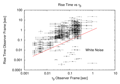
Figure 1: Minimum variability time scale versus rise time in the Observer frame. The rise times are taken from Table 3 of Bhat et al. (2012). The line represents the locus where $\tau_{\beta}$ = rise time. We identify the area below the line with white noise. The data are expected to press up against the line from above but not to cross it.

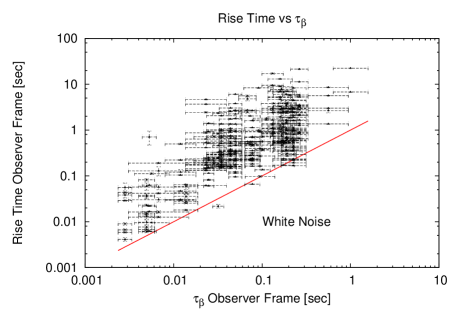
Figure 2: Minimum variability time scale versus rise time in the Observer frame. We have removed all pulses (20) with rise times smaller than the light curve bin width.

Note that in Fig. 2 the white noise region has been vacated by all but seven points and none of the pulse rise times above the equality line have been disturbed by the bin width cut. For the seven points that remain beneath the equality line, we show in Table 1 that six are within one sigma of the equality line.

We make one other point regarding the pulse rise times in Fig. 1 and Fig. 2, in particular regarding the size of the uncertainties. Of the 379 pulse rise times reported by Bhat et al. (2012) and used for this meta-analysis, 301 have uncertainties smaller than the binning of the light curve, in some cases hundreds or thousands of times smaller. We argue that a conservative estimate of the uncertainties for the pulse rise times should be no smaller than a bin width. Thus, we add in quadrature a bin width (as reported in Table 3 of Bhat et al. (2012)) to the rise time uncertainties (also reported in Table 3 of Bhat et al. (2012)) and plot the result in Fig. 3.

In Fig. 4 we plot only the smallest rise times for each GRB against $\tau_{\beta}$. We argue that by rejecting pulse rise times smaller than light curve bin widths and by folding rise time uncertainties with a bin width we get strong evidence that Bhat et al. (2012) and MacLachlan et al. (2012) have tracked the same physical observables over approximately three orders of magnitude using independent methods.

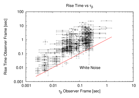
Figure 3: Minimum variability time scale versus rise time in the Observer frame as in Fig. 2. We have folded a single bin width into the rise time uncertainties.

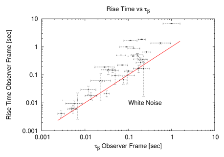
Figure 4: Minimum variability time scale versus rise time in the Observer frame as in Fig. 3 but with only smallest rise times included. Note that the equality line between $\tau_{\beta}$ and rise time marks a boundary between scaling processes and white noise and gives substance to the interpretation of the minimum variability time scale.

3 Results and Discussion

For a large sample of short and long Fermi GBM bursts, MacLachlan et al. (2012) used a technique based on wavelets to determine the minimum variability time scale, $\tau_{\beta}$. The authors associate this time scale with a transition from red-noise processes to parts of the power spectrum dominated by white noise or random noise components. Accordingly, the authors note that this time scale is the shortest resolvable variability time for physical processes intrinsic to the GRB. In addition, histograms of the values of $\tau_{\beta}$ for long and short GRBs were shown to exhibit a clear temporal offset in the mean $\tau_{\beta}$ values for long and short GRBs.

In a separate analysis, using a particular functional form for pulse shapes, Bhat et al. (2012) have extracted an extensive set of key pulse parameters such as rise times, decay times, widths (FWHM), and times since trigger for a host of bright GRBs detected by Fermi/GBM. Using the FWHM values, these authors also reported a significant temporal offset between the mean values for long and short GRBs.

Although neither group offers a concrete explanation for the temporal difference between the distributions of long and short GRBs, it is noteworthy that they arrive at a result which is quantitatively in good agreement with one another, especially having used independent approaches. Both sets of analyses also suggest scaling trends between characteristic timescales. In the case of minimum variability timescales the trend is between $\tau_{\beta}$ and the duration of the burst, typically denoted by $T_{90}$. For the pulse-shape analysis, the trend is more readily evident and is demonstrated through a number of positive correlations involving key parameters such as rise times, decay times and FWHM times.

It is relatively straightforward to interpret the scaling trends in terms of the internal shock model in which the basic units of emission are assumed to be pulses that are produced via the collision of relativistic shells emitted by the central engine. In the case of the pulse-fitting method this is essentially the default assumption. Indeed, Quilligan et al. (2002) in their study of the brightest BATSE bursts with $T_{90}>2$ sec were the first to demonstrate this explicitly by identifying and fitting distinct pulses and showing a strong positive correlation between the number of pulses and the duration of the burst. More recent studies, Bhat & Guiriec (2011); Hakkila & Cumbee (2008); Hakkila & Preece (2011) have provided further evidence for the pulse paradigm view of the prompt emission in GRBs.

The wavelet analysis does not, however, rely on identifying distinct pulses but instead uses the multiresolution capacity of the wavelet technique to resolve the smallest temporal scale present in the prompt emission. Nonetheless, as MacLachlan et al. (2012) have demonstrated, if the smallest temporal scale is due to pulse emissions, then we can still get a measure of the upper bound on the number of pulses in a given burst through the ratio $T_{90}/\tau_{\beta}$. In the simple model in which a pulse is produced every time two shells collide, the ratio $T_{90}/\tau_{\beta}$, should show a correlation with the duration of the burst. Indeed, this correlation was reported by MacLachlan et al. (2012).

The similar trends of scaling demonstrated by these two methods, not only suggest the robustness of both methods, but also point, perhaps more importantly, to an underlying interconnection between key parameters extracted by the two techniques. In other words, the minimum variability time scale extracted by the wavelet technique is directly related to key pulse time parameters such as rise times (as depicted in Fig. 4), under suitably controlled pulse-fitting methods.

4 CONCLUSIONS

Through a meta-analysis of results presented by Bhat et al. (2012) and by MacLachlan et al. (2012), we have studied the relationship between key parameters that describe the temporal properties of a sample of prompt-emission light curves for long and short-duration GRBs detected by the Fermi/GBM mission. We compare the minimum variability timescale extracted through a technique based on wavelets, with the pulse-time parameters extracted through a pulse-fitting procedure. Our main results are summarized as follows:

a) Both methods indicate a temporal offset between short and long-duration bursts. The quantitative agreement between the two methods is quite good.

b) Both methods point to scaling trends between characteristic timescales. In the case of the pulse-fitting method the scaling appears to involve parameters such as rise times, FWHM, and pulse intervals. For the wavelet technique, the scaling involves a correlation between the minimum variability time scale and the duration of the bursts.

c) By demonstrating a strong positive correlation between $\tau_{\beta}$ and the rise time of the shortest fitted pulses, we provide for the first time, a direct link between the shortest resolvable temporal structure in a GRB light curve with that of a key pulse profile parameter.

d) By combining the two techniques, we have shown that one can arrive at a much tighter demarcation of the boundary between the power spectrum domains that separate red noise and white noise processes.

5 ACKNOWLEDGEMENTS

The NASA grant NNX11AE36G provided partial support for this work and is gratefully acknowledged. The authors, in particular GAM and KSD, acknowledge very useful discussions with Jon Hakkila and Narayan Bhat.

References

- Bhat & Guiriec (2011) Bhat, P. N., & Guiriec, S. 2011, BASI, 39, 471
- Bhat et al. (2012) Bhat, P. N. et al. 2012, ApJ., 744, 141 (online-version)
- Hakkila & Cumbee (2008) Hakkila, J. & Cumbee, R. 2008, arXiv:0901.3171v1 [astro-ph.HE].
- Hakkila & Nemiroff (2009) Hakkila, J. & Nemiroff, R. J. 2009, ApJ., 705, 372
- Hakkila & Preece (2011) Hakkila, J. & Preese, R. 2011, ApJ., 740, 104
- MacLachlan et al. (2012) MacLachlan, G. A., et al. 2012, arXiv:1201.4431v2 [astro-ph.HE]
- Nemiroff (2000) Nemiroff, R. J. et al. 2000, ApJ., 544, 805
- Nemiroff (2012) Nemiroff, R. J. 2012, MNRAS, 419, 1650
- Norris et al. (2005) Norris, J. P. et al. 2005, ApJ., 627, 324
- Quilligan et al. (2002) Quilligan, F., et al. 2002, A.& A., 385, 377