A Multi-wavelength Study of the Sunyaev–Zel’dovich Effect in the Triple-Merger Cluster MACS J0717.5+3745 with MUSTANG and Bolocam

Abstract

We present 90, 140, and 268 GHz sub-arcminute resolution imaging of the Sunyaev-Zel’dovich effect (SZE) in the disturbed, intermediate redshift ($z=0.5458$) galaxy cluster MACS J0717.5+3745, a triple-merger system comprising four distinct, optically-detected subclusters. Our 90 GHz SZE data result in a sensitive, 34 $\,\mu$Jy beam^-1 map of the SZE at 13^′′ effective resolution using the MUSTANG bolometer array on the Green Bank Telescope (GBT). Our 140 and 268 GHz SZE imaging, with resolutions of 58^′′ and 31^′′ and sensitivities of 1.8 and 3.3 mJy beam^-1, respectively, was obtained through observations from the Caltech Submillimeter Observatory using Bolocam. We compare these maps to a two-dimensional pressure map derived from Chandra X-ray observations. Our MUSTANG SZE data confirm previous indications from Chandra of a pressure enhancement due to shock-heated, $\gtrsim 20\,{\rm keV}$ gas immediately adjacent to extended radio emission seen in low-frequency radio maps of this cluster. MUSTANG also detects pressure substructure that is not well-constrained by the Chandra X-ray data in the remnant core of a merging subcluster. We find that the small-scale pressure enhancements in the MUSTANG data amount to $\sim 2$% of the total pressure measured in the 140 GHz Bolocam observations. The X-ray inferred pseudo-pressure template also fails on larger scales to accurately describe the Bolocam data, particularly at the location of the subcluster with a remnant core known to have a high line of sight optical velocity of $\sim 3200$ km s^-1. Our Bolocam data are adequately described when we add an additional component—not described by a thermal SZE spectrum—to the X-ray template coincident with this subcluster. Using flux densities extracted from our model fits, and marginalizing over the X-ray spectroscopic temperature constraints for the region, we fit a thermal + kinetic SZE spectrum to our Bolocam data and find that the subcluster has a best-fit line-of-sight proper velocity $v_{z}=3600^{+3440}_{-2160}$ km s^-1, in agreement with the optical velocity estimates for the subcluster. The probability $v_{z}\leq 0$ given our measurements is 2.1%. Repeating this analysis using flux densities measured directly from our maps results in a 3.4% probability $v_{z}\leq 0$. We note that this tantalizing result for the kinetic SZE is on resolved, subcluster scales.

1. Introduction

Massive ($\gtrsim 10^{15}~{}M_{\odot}$) galaxy clusters are the largest gravitationally-bound objects in the universe and their formation is thought to be driven by mergers of smaller clusters in what are the most energetic events to take place since the big bang (Sarazin 2005). Our understanding of the astrophysics of mergers and the intracluster medium (ICM) has traditionally been advanced through X-ray observations (e.g., McNamara et al. 2005; Markevitch & Vikhlinin 2007), which are sensitive to both the density and the temperature of the gas. However, sensitive, high angular resolution imaging of the Sunyaev-Zel’dovich effect (SZE) has recently become possible (e.g., Kitayama et al. 2004; Nord et al. 2009; Mason et al. 2010; Korngut et al. 2011; Plagge et al. 2012), helping to yield a more complete view of the complex processes in the ICM, particularly at high redshift.

The SZE is due to inverse Compton scattering of cosmic microwave background (CMB) photons to higher energies on average by hot electrons in the ICM (Sunyaev & Zel’dovich 1972); for reviews of the SZE, including its thermal and kinetic components, see Birkinshaw (1999) and Carlstrom et al. (2002). The SZE complements X-ray and optical observations, offering some of its own unique advantages. First, unlike intrinsic emission mechanisms (e.g., X-ray, optical, and radio) from a cluster, the SZE does not suffer cosmological surface brightness dimming ($\propto(1+z)^{-4}$). Second, the thermal SZE (tSZE) is proportional to the line-of-sight integrated thermal electron pressure, while X-ray observations are sensitive to the ICM density-squared. The different line-of-sight dependences of X-ray and SZE data allow one to infer information about the line-of-sight properties of the ICM. Third, there is the potential to constrain the component of ICM proper velocity along the line-of-sight using a Doppler shift of the CMB known as the kinetic SZE (kSZE). The combination of the SZE observations with those from radio, optical, X-ray, and other wave bands can provide a more complete understanding of cluster mergers and other astrophysical processes.

A particularly striking example of a cluster merger is MACS J0717.5+3745 (Ebeling et al. 2001; Edge et al. 2003). At a redshift $z=0.5458$, MACS J0717.5+3745 is the hottest member of the MAssive Cluster Survey (MACS; Ebeling et al. 2001) at $z>0.5$; Ebeling et al. (2007) report an average X-ray spectroscopic temperature $\mbox{$k_{\mbox{\tiny B}}$}\mbox{$T_{\mbox{\tiny X}}$}=11.6\pm 0.5\,{\rm keV}$, determined within an overdensity of 1000 times the critical density of the universe and by excluding the central 70 kpc of the cluster, and a velocity dispersion $\sigma\sim 1660$ km s^-1 within a 1 Mpc aperture. Optical imaging and spectroscopy have shown that the cluster is located at the end of a $4\,h_{70}^{-1}\,{\rm Mpc}$ long filamentary overdensity of galaxies (Ebeling et al. 2004), consistent with the expectation that clusters form at intersections in the cosmic web. Ma et al. (2008, 2009) have also shown that the cluster itself comprises four distinct groups of galaxies and appears to be a rare triple-merger in progress. Low-frequency radio images (Edge et al. 2003; van Weeren et al. 2009; Bonafede et al. 2009) show the presence of diffuse radio emission as well, indicative of a radio relic or halo.

In this paper we compare multi-wavelength observations of the SZE with X-ray, radio, and lensing observations. Our SZE imaging data include 90 GHz data collected with the MUSTANG bolometer array (Dicker et al. 2008) on the Green Bank Telescope (GBT), along with 140 and 268 GHz data collected with Bolocam (Haig et al. 2004) from the Caltech Submillimeter Observatory (CSO). The MUSTANG data have a resolution of $13^{\prime\prime}$—due to the $8^{\prime\prime}.5$ instrument resolution and $10^{\prime\prime}$ smoothing of the maps—and a sensitivity of $\sim 34$ $\,\mu$Jy beam^-1 within a central radius of $\sim 40^{\prime\prime}$. The Bolocam data have resolutions of $58^{\prime\prime}$ and $31^{\prime\prime}$ at 140 and 268 GHz—on opposite sides of the null in the tSZE spectrum—and have sensitivities of 1.8 and 3.3 mJy beam^-1, respectively. The Bolocam data probe scales as large as 14^′, while the more sensitive MUSTANG data do not reliably probe scales $>1^{\prime}$. Additionally, we compare these observations to a CARMA/SZA 31 GHz observation of this cluster. The short baselines of CARMA/SZA probe scales up to 12^′ with a 2^′ synthesized beam. The longer baselines of the CARMA/SZA, with a $\sim 10^{\prime\prime}$ synthesized beam, lack the sensitivity to detect SZE on these scales, but provide constraints on the locations and spectral indices of the potentially contaminating compact radio source population. We therefore use the CARMA/SZA data to place constraints on the large angular scale cluster properties (the “bulk” SZE flux) and to help constrain contamination by radio sources.

The organization of the paper is as follows. In Section 2, we provide an overview of results from previous optical, low frequency radio, and X-ray observations of MACS J0717.5+3745. In Section 3, we describe the MUSTANG, Bolocam, CARMA/SZA, and Chandra X-ray observations and data reduction. Section 4 gives the details of modelling of the SZE observable properties and the X-ray data products used in this analysis. In Section 5, we use the Bolocam 140 and 268 GHz data, along with our X-ray temperature constraints, to infer the peculiar velocity of one subcluster component with a spectrum that is not well described by the thermal SZE alone, and we compare these estimates to those for the most massive subcluster in this system. We present our conclusions from this multi-wavelength SZE study in Section 6. Throughout this paper, we adopt a flat, $\Lambda$-dominated cosmology with $\Omega_{\mbox{\tiny\rm M}}=0.3$, $\Omega_{\Lambda}=0.7$, and $H_{0}=70$ km s^-1 Mpc^-1 consistent with recent Wilkinson Microwave Anisotropy Probe (WMAP) results (Komatsu et al. 2009, 2011).

2. Previous Analyses of MACS J0717.5+3745

MACS J0717.5+3745, a complex merging system discovered in the MACS survey (Ebeling et al. 2001, 2007), is among the best-studied massive clusters at redshift $z>0.5$, with observations spanning a broad range of the electromagnetic spectrum. In support of our multi-wavelength SZE study, we compare our MUSTANG and Bolocam observations to X-ray, optical, and low frequency radio data, and to the results of many studies that have relied upon these data.

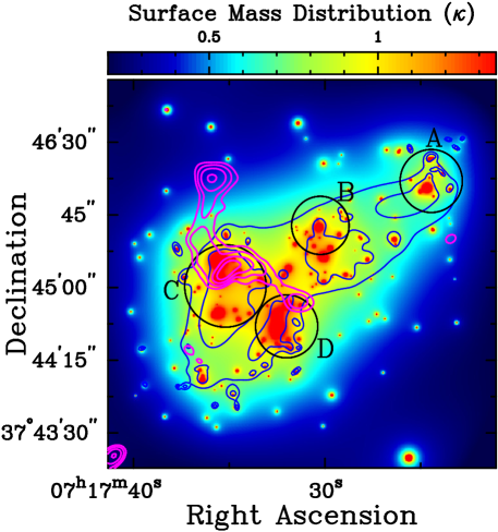
Figure 1.— Surface mass distribution in units of the critical surface density (convergence, $\kappa$) for MACS J0717.5+3745 determined by Zitrin et al. (2009) through strong lensing measurements (color image). Black circles correspond to the four main peaks in the cluster light distribution as identified by Ma et al. (2009). The magenta contours (3$\sigma$, 6$\sigma$, 12$\sigma$, 24$\sigma$) reproduce the 610 MHz GMRT data in van Weeren et al. (2009). The blue contours reproduce the (5,7)$\times 10^{10}~{}M_{\odot}\,\rm arcsec^{-2}$ contours in Limousin et al. (2012). We note that recent redshift information reported in Limousin et al. (2012) reduces the overall mass estimate, but that the features otherwise show broad agreement.

From X-ray and optical analyses, Ma et al. (2009) identify four distinct components in MACS J0717.5+3745. These subclusters are shown in Figure 1 on the strong lensing data from Zitrin et al. (2009), who note that this cluster has the largest known Einstein radius, $\theta_{e}\sim 55^{\prime\prime}$. Zitrin et al. (2009) cite this large Einstein radius and the shallow surface mass distribution as further evidence that the cluster is disturbed, while Limousin et al. (2012) characterize this as “one of the most disturbed clusters presently known” in their recent strong lensing analysis. We note that the lensing analysis of Zitrin et al. (2009) assumed a redshift $z\sim 2.5$ for the primary lensed system. The recent redshift information reported in Limousin et al. (2012) entails a shift in the normalization of the surface mass distribution $\kappa$, reducing the overall mass estimate for MACS J0717.5+3745. The analysis presented here only relies on the fact that lensing has located four mass peaks, and that they show good agreement with the regions optically identified by Ma et al. (2009).

Ma et al. (2009) provide the following interpretation of the four dominant mass components in this merging cluster. Subcluster A is the least massive and is likely falling back into the main cluster from the NW, after having passed through once already. Subclusters B and D are likely remnant cores that survived an initial encounter in a merger along an axis inclined much more toward the line of sight. Subcluster C, which is the most massive component in MACS J0717.5+3745, exhibits good X-ray/optical alignment and is most likely the disturbed core of the main cluster. Ma et al. (2009) also report the line-of-sight (optical) spectroscopically-determined velocities for subclusters A, B, C, and D as $(v_{\mbox{\tiny A}},v_{\mbox{\tiny B}},v_{\mbox{\tiny C}},v_{\mbox{\tiny D}})=(+278^{+295}_{-339},+3238^{+252}_{-242},-733^{+486}_{-478},+831^{+843}_{-800})$ km s^-1. We note the remarkably high line-of-sight velocity for subcluster B ($\gtrsim 0.01~{}c$).

The Giant Metrewave Radio Telescope (GMRT) observed MACS J0717.5+3745 at 610 MHz for a total of 4 hr (van Weeren et al. 2009). These GMRT observations reveal a powerful radio halo with a spectral index $\alpha=-1.25$, as well as a 700 kpc wide substructure identified as a radio relic by van Weeren et al. (2009). According to van Weeren et al. (2009), the progenitor of the radio relic is likely a merger-driven shock wave within the cluster which has accelerated electrons via the diffuse shock acceleration (DSA) mechanism. The radio substructure brackets the high-temperature regions of the ICM (see Figure 3) and is oriented perpendicular to the merger axes and large-scale filament, which supports the relic scenario.

Bonafede et al. (2009) performed high- and low-resolution observations of MACS J0717.5+3745 in full polarization mode with the Very Large Array (VLA), at frequencies spanning 1.365–4.885 GHz. They measure polarizations up to 20% in the radio substructure and find no sharp discontinuity of the $E$-vectors between the large-scale halo and the putative relic, which is expected for a true relic (Clarke & Ensslin 2006). Bonafede et al. (2009) find that the observed lack of Faraday rotation does not agree with the expectation for a relic produced by a merger shock near the center of a cluster. Lastly, there is no steepening of the spectral index across the short axis of the substructure, as would be expected of a radio relic following a merger. Thus, Bonafede et al. argue that the substructure is not a radio relic, but rather a bright, polarized filament connected with the radio halo.

The competing interpretations of the low frequency radio data both support the hypothesis that merger activity has produced a relativistic, nonthermal component to the ICM of MACS J0717.5+3745, not seen in the Chandra X-ray observations implying it has a relatively low density typical of radio relics/halos.

3. Observations and Data Reduction

3.1. MUSTANG Observations

MUSTANG is a 64 element bolometer array operating at 90 GHz on the 100-m GBT with a resolution of 8.$\!{}^{\prime\prime}$5. For more information about MUSTANG, refer to Dicker et al. (2008).

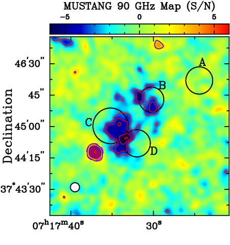
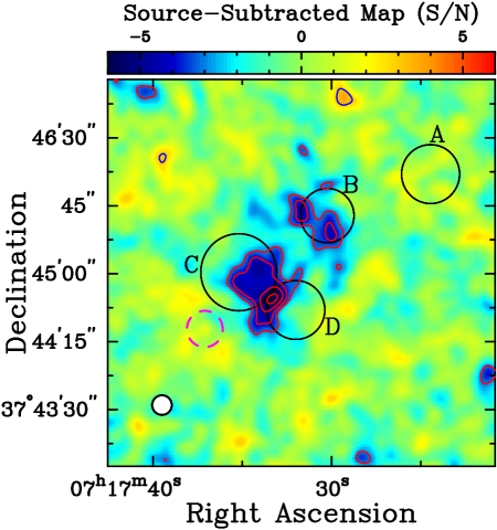
Figure 2.— MUSTANG maps of MACS J0717.5+3745 with contours starting at $\pm 3\sigma$, spaced at 1$\sigma$ intervals for the decrement (red) and at 3$\sigma$ intervals for the positive signal (blue). The effective resolution of the map, which is 13^′′ due to the instrument beam ($8.\!^{\prime\prime}5$ FWHM) and image smoothing with a 10^′′ FWHM Gaussian, is depicted in the lower left corner of each map. The noise level in the inner $\sim 40^{\prime\prime}$ radial region is 34 $\,\mu$Jy beam^-1, and is 53 $\,\mu$Jy beam^-1 within the inner 3^′ radial region. Due to our map-making process, features on angular scales $\gtrsim 1^{\prime}$ are attenuated. The largest extended SZE signal in this high-pass filtered view is located near subclusters C and D, while a secondary SZE feature is also detected near B (see the text for details). Upper: MUSTANG map of MACS J0717.5+3745  before modelling and removal of the foreground source. Lower: MUSTANG map with foreground radio source modelled and removed from the time-ordered data. Location of the removed source is marked with a magenta, dashed circle. Contours for the decrement are the same as above, but are now spaced at 1$\sigma$ intervals for positive emission in the radio source-subtracted map (starting at +3$\sigma$).

Between 2010 October and 2012 February we observed MACS J0717.5+3745 for a total of 15 hr on source over the course of 11 sessions. Observations were carried out using an on-the-fly scan strategy similar to that described in Mason et al. (2010) and Korngut et al. (2011). For this, we move the telescope in a “lissajous daisy” pattern with a $3^{\prime}$ radius and slowly nutate the center of the daisy pattern to increase the coverage. Seven different pointing centers were used to further expand the coverage of the central part of the cluster.

MUSTANG data were reduced and calibrated according to procedures described in Mason et al. (2010) and Korngut et al. (2011). The overall measurement errors and uncertainties in both the temperatures of Uranus and Mars, and the shape of the GBT’s beam, limit our flux calibration to 10% uncertainty in the absolute flux scale. The data presented here are fully common-mode subtracted; that is, we remove the instantaneous signal common to the detector array. This has the benefit of removing atmospheric noise at the expense of attenuating signals from features with angular scales $\gtrsim 1^{\prime}$. This limits the spatial dynamic range of the MUSTANG data presented here. Two largely independent implementations of the map-making pipeline exist, and have different approaches for common-mode subtraction, residual noise filtering, and data flagging. The features in Figure 2 are recovered by both pipelines with consistent brightness levels.

The MUSTANG map in the top panel of Figure 2 has three main features, two due to the cluster and one due to a foreground elliptical galaxy. The two extended SZE decrements have peaks of $-169\pm 37$ and $-188\pm 30$ $\,\mu$Jy beam^-1, and are detected at 4.6 and 6.2$\sigma$ significance at their peaks. The foreground galaxy, which is not co-spatial with the SZE in the map, is resolved by MUSTANG and has an integrated flux density of $+2.8\pm 0.2$ mJy (13.7$\sigma$ at the peak) and an extended shape of $14.4^{\prime\prime}\times 16.1^{\prime\prime}$. The source is also detected at other wavelengths, including Chandra, GMRT, VLA (FIRST/NVSS), CARMA/SZA, and optical observations to name a few.

The radio sources detected in our maps at $>$3$\sigma$, such as the aforementioned foreground galaxy in the MACS J0717.5+3745 field, can be modelled and subtracted from our data. Provided the source has a significant detection, an initial estimate of the position, flux, and, if appropriate, shape of the source can be estimated from a first-pass map of the MUSTANG data. This model is then subtracted from the time ordered data before making a new, point-source subtracted map (see lower panel of Figure 2). If necessary, the source model convolved by the beam can be updated to better remove any residual flux after the first-pass point source removal. This method has the advantage over simply subtracting the source from the map in that the true shape and size of the source can be recovered while accounting for non-linearities of the map-making routine (e.g., the influence of the source on the common mode subtraction and weight estimates). One drawback to this method is that it subtly alters the noise estimate in the S/N maps shown in Figure 2. However, as we show in §4.2.1, this has a negligible impact on flux estimates from the MUSTANG data.

3.2. Bolocam Observations

Bolocam is a 144 element bolometer array capable of operation at either 140 or 268 GHz. Operating from the 10-m CSO, it provides resolutions of 58^′′ and 31^′′ at 140 and 268 GHz, respectively, over an 8^′ instantaneous field of view. A complete description of the Bolocam instrument can be found in Haig et al. (2004).

We used Bolocam to observe MACS J0717.5+3745 for a total of 12.5 hours at 140 GHz (6 hr in 2010 February and 6.5 hr in 2010 October) and for a total of 8 hr at 268 GHz (3 hr in 2011 September and 5 hr in 2011 November). Due to the large instantaneous field of view, these data have uniform coverage over the roughly $4^{\prime}\times 4^{\prime}$ region in which we are interested, with noise levels of 1.8 and 3.3 mJy beam^-1 for the 140 and 268 GHz data, respectively. These data were reduced according to the procedures described in Sayers et al. (2011) using the updated calibration model of Sayers et al. (2012). We briefly summarize the reduction below.

We used frequent observations of the nearby quasars to obtain pointing corrections accurate to 5^′′. We determined our flux calibration, with 5% and 10% uncertainties at 140 and 268 GHz, using observations of Uranus and Neptune. We subtracted atmospheric noise from the data via a common-mode template and a time-stream high-pass filter with a characteristic frequency of 250 mHz. The largest scales recovered after filtering (at either observational frequency) are 14^′. This noise subtraction also removes cluster signal, and we determined the effective transfer function of our data processing by reverse-mapping a simulated cluster profile into our time-stream data and running it through the entire pipeline (for details see Sayers et al. 2011). We note that the transfer functions were determined independently for the 140 and 268 GHz data, and are slightly different from each other.

This data reduction results in a high-pass filtered image of the astronomical signal. Therefore, prior to comparing any model of the SZE signal to our data we must first convolve the model with both our point spread function (PSF) and the data-processing transfer function. Model fitting is otherwise straightforward, and the map noise is approximately white and is well described by a diagonal noise covariance matrix. Alternatively, we can also deconvolve the effects of the data-processing transfer function to obtain an unbiased image of the astronomical signal (aside from the effects of our PSF). Although the deconvolution amplifies the large scale noise in the image, it allows us to directly compute total flux densities from within an arbitrary aperture. In this paper, we exclusively use our processed data maps for all SZE model fitting to our Bolocam data, and we use our deconvolved data maps to obtain aperture-integrated fluxes which we compare to the model-fit values. We note that in both cases, in order to fully account for any non-idealities in our noise, we determine all of our uncertainty estimates via 1000 statistically independent noise realizations.

3.3. CARMA/SZA Observations

The Sunyaev–Zel’dovich Array (SZA; Muchovej et al. 2007) is a subarray comprising eight 3.5 m antennae in the Combined Array for Millimeter-wave Astronomy (CARMA). CARMA, including the SZA, is located at an altitude of 2200 m in the Inyo Mountains of California. The SZA is capable of observing in three modes: separately, paired with the larger 6.1 and 10 m antennae of CARMA, and as part of the full CARMA 23-element heterogeneous array (see Plagge et al. 2012, for recent observations with the full array at 90 GHz).

Our observations use the 31 GHz SZA as an independent system in a compact configuration sensitive to 1^′–6^′ scales with a $10.\!^{\prime}5$ FWHM primary beam, which determines the field of view (for more details see Muchovej et al. 2007). The spatial filtering of the interferometer allows small scale positive point source emission to be separated from the large-scale, negative SZE signal at these frequencies (for an example in a similar context see Reese et al. 2002). The compact configuration provides two outrigger antennae (for a total of 13 of the 28 baselines) that probe $\sim 10\arcsec$ scales, though the rms noise level ($\sim 0.2$ mJy) is not low enough to measure the SZE, which is a factor of $\sim 6\times$ lower at 31 GHz than at 90 GHz. Our SZA 31 GHz observations are reduced using the pipeline described in Muchovej et al. (2007), and were calibrated using the Rudy (1987) model for Mars. The synthesized beam of the inner six elements of the SZA, which is in a compact configuration to optimize cluster imaging on large scales, was $118\times 131^{\prime\prime}$ for these observations. We use the SZA observations to constrain the bulk, arcminute-scale SZE decrement and to leverage the spectral indices of potential contamination by compact radio sources.

3.4. Chandra X-Ray Observations

The Chandra X-ray Observatory made two ACIS-I observations of MACS J0717.5+3745 for a total exposure time of 81 ks (ObsIDs 1655 and 4200). We have reduced the data using CIAO version 4.3 and calibration database (CALDB) version 4.4.5. Starting with the level 1 events file, standard corrections are applied along with light curve filtering and other standard processing (for details see Reese et al. 2010). A wavelet-based detection algorithm is used to find point sources, which is then used as the basis of our point source mask. We discuss the data products we generate from our calibrated Chandra X-ray data in Section 4.1.

4. Thermal Analysis of the ICM

We do not expect the assumption of spherical symmetry to be an accurate description of this merging cluster on subarcminute scales. This motivates the use of X-ray data to produce a two-dimensional template for the tSZE signal in our observations. X-ray data can be used to infer electron pressure, $\mbox{$P_{\mbox{\scriptsize e}}$}=\mbox{$n_{\mbox{\tiny e}}$}\mbox{$k_{\mbox{\tiny B}}$}\mbox{$T_{\mbox{\tiny e}}$}$, the thermodynamic property to which the tSZE is linearly sensitive. X-ray spectroscopy provides a measure of temperature $k_{\mbox{\tiny B}}$$T_{\mbox{\tiny e}}$, while X-ray imaging (i.e. surface brightness $S_{\mbox{\tiny X}}$) is proportional to the line of sight integral of the electron density squared, $n^{2}_{\mbox{\tiny e}}$, times the X-ray cooling function $\Lambda_{\mbox{\tiny ee}}$ ($\propto\mbox{$T_{\mbox{\tiny e}}$}^{1/2}$). Resolved temperature and pseudo-pressure maps, so-called because X-ray data alone do not constrain the line-of-sight depth of the cluster, are common in detailed X-ray studies of ICM thermodynamics (see e.g., Ma et al. 2009; Russell et al. 2010).

The intensity of the tSZE is

$$\Delta\mbox{$I_{\mbox{\tiny tSZE}}$}=I_{0}\,g(\nu,\mbox{$T_{\mbox{\tiny e}}$})\,y,$$ (1)

where the primary CMB intensity normalization is $I_{0}=2(\mbox{$k_{\mbox{\tiny B}}$}\mbox{$T_{\mbox{\tiny CMB}}$})^{3}(hc)^{-2}=2.7033\times 10^{8}$ Jy sr^-1 ($=22.87~{}\rm Jyarcmin^{-2}$) and $T_{\mbox{\tiny CMB}}$ is the temperature of the CMB. Following Carlstrom et al. (2002), the function $g(\nu,\mbox{$T_{\mbox{\tiny e}}$})$ describes the frequency dependence of the tSZE. We include the relativistic corrections of Itoh et al. (1998) and Itoh & Nozawa (2004). The Compton-$y$ parameter in Equation 1 is defined as

$$y\equiv\frac{\mbox{$\sigma_{\mbox{\tiny T}}$}}{\mbox{$m_{\mbox{\tiny e}}c^{2}$}}\int\!\mbox{$n_{\mbox{\tiny e}}$}\mbox{$k_{\mbox{\tiny B}}$}\mbox{$T_{\mbox{\tiny e}}$}\,d\ell=\frac{\mbox{$\sigma_{\mbox{\tiny T}}$}}{\mbox{$m_{\mbox{\tiny e}}c^{2}$}}\int\!\mbox{$P_{\mbox{\scriptsize e}}$}\,d\ell,$$ (2)

where $\sigma_{\mbox{\tiny T}}$ is the Thomson cross section, $m_{\mbox{\tiny e}}c^{2}$ is the rest energy of the electron, the integration is along the line-of-sight $\ell$, and we have used the ideal gas law ($\mbox{$P_{\mbox{\scriptsize e}}$}=\mbox{$n_{\mbox{\tiny e}}$}\mbox{$k_{\mbox{\tiny B}}$}\mbox{$T_{\mbox{\tiny e}}$}$).

4.1. X-ray Data Products

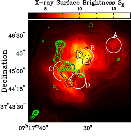
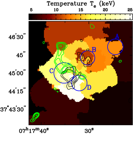
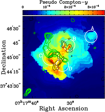
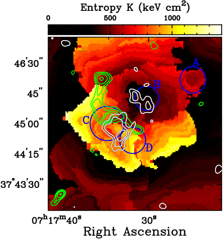
Figure 3.— Comparison between MUSTANG SZE detections and the thermodynamic properties of MACS J0717.5+3745 inferred from Chandra X-ray data. MUSTANG SZE detections from lower panel of Figure 2 are overlaid (black contours, except for lower right panel). GMRT radio contours are overlaid in green (reproduced from van Weeren et al. (2009)). Upper left: X-ray surface brightness map (shown on a scale $\propto\sqrt{\mbox{$S_{\mbox{\tiny X}}$}}$). Upper right: X-ray temperature map. The MUSTANG peak detections of the SZE are located both where the hottest gas is found in the Chandra data (C and D) and at the location of subcluster B. Lower left: pseudo Compton-$y$ map. This rescaling of the pseudo pressure map aids in the interpretation of the SZE data, and serves as a two-dimensional template for modelling the tSZE (Section 4.2). Lower right: map of the entropy parameter $K=\mbox{$k_{\mbox{\tiny B}}$}\mbox{$T_{\mbox{\tiny e}}$}/\mbox{$n_{\mbox{\tiny e}}$}^{2/3}$ in MACS J0717.5+3745.

To build the tSZE template, we first bin the reduced Chandra data using contbin (Sanders 2006), which uses the X-ray surface brightness to select regions of the image large enough to obtain a desired S/N level. For the temperature maps, we chose regions of the X-ray surface brightness image with $\rm S/N>45$. Each bin provides independent measurements of surface brightness $S_{\mbox{\tiny X}}$, temperature $k_{\mbox{\tiny B}}$$T_{\mbox{\tiny e}}$, and metallicity $Z$. For the spectral analysis to determine $k_{\mbox{\tiny B}}$$T_{\mbox{\tiny e}}$ and $Z$, data extracted from each region are fit jointly using spectra and response files produced from each individual observation. Regions containing point sources are excluded from the extraction of the spectra and computation of the response files. XSPEC is used to perform a joint spectral fit to both data sets over the 0.7–7.0 keV energy range, linking temperature and metallicity between the data sets but allowing the normalizations to vary. The masked regions of the data product maps are then filled in via a simple, bilinear interpolation scheme.

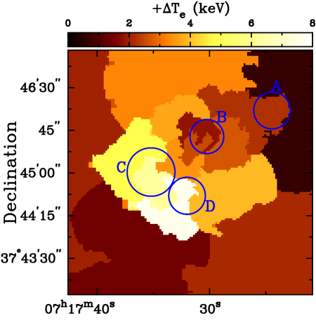
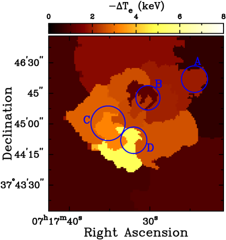
Figure 4.— $\pm 1\sigma$ statistical error bars for the temperature map presented in Figure 3. Typical errors bars are $+3/-2$ keV for most regions, except for the hottest regions where subclusters C and D are interacting and the gas temperature is significantly out of Chandra’s energy band.

Using the Chandra-derived $k_{\mbox{\tiny B}}$$T_{\mbox{\tiny e}}$ and $Z$ maps, we compute the cooling function, $\mbox{$\Lambda_{\mbox{\tiny ee}}$}(\mbox{$T_{\mbox{\tiny e}}$},Z)$, as a function of map bin, and use it to compute a line-of-sight integrated pseudo-pressure map, where

$$\int\mbox{$P_{\mbox{\scriptsize e}}$}\,d\ell\propto\mbox{$k_{\mbox{\tiny B}}$}\mbox{$T_{\mbox{\tiny e}}$}\sqrt{\frac{4\pi(1+z)^{3}\mbox{$S_{\mbox{\tiny X}}$}\ell}{\mbox{$\Lambda_{\mbox{\tiny ee}}$}(\mbox{$T_{\mbox{\tiny e}}$},Z)}}.$$ (3)

Here $S_{\mbox{\tiny X}}$ (in $\rm counts~{}cm^{-2}~{}s^{-1}~{}sr^{-1}$) is the X-ray surface brightness, and $\mbox{$\Lambda_{\mbox{\tiny ee}}$}(\mbox{$T_{\mbox{\tiny e}}$},Z)$ (in $\rm counts~{}cm^{3}~{}s^{-1}$) contains the additional factor of $(1+z)^{-1}$ required by cosmological dimming, due to redshifting of the photon energy. The factor $\ell$ is an effective electron depth of the cluster along the line-of-sight, taken to be a single value over the map. Surprisingly, this is consistent with the average slopes found when using simple $\beta$-models to describe the density and pressure profiles (Sarazin 1988; LaRoque et al. 2006; Plagge et al. 2010); a justification for this assumption may be found in the Appendix. We note that this does not imply pressure is constant along the line of sight, but rather that the average ratio of Compton-$y$ to $\sqrt{\mbox{$S_{\mbox{\tiny X}}$}}$ is approximately constant azimuthally.

We refer to this X-ray template for the tSZE, which is simply a rescaling of the X-ray pseudo-pressure map by $\sqrt{\ell}$, as a “pseudo Compton-$y$ map.” In constructing this, we have assumed Equation 2 can be approximated as $y=\mbox{$\sigma_{\mbox{\tiny T}}$}/(\mbox{$m_{\mbox{\tiny e}}c^{2}$})\int\mbox{$P_{\mbox{\scriptsize e}}$}d\ell\approx\mbox{$\sigma_{\mbox{\tiny T}}$}/(\mbox{$m_{\mbox{\tiny e}}c^{2}$})\mbox{$P_{\mbox{\scriptsize e}}$}\ell$. The key ingredient to building this template is the use of an SZE measurement on large angular scales to infer $\ell$. By using the integrated SZE flux, $\mbox{$Y_{\mbox{\tiny tSZE}}$}=\int y\,d\Omega$, from the Bolocam 140 GHz and SZA 31 GHz observations to normalize the sum over the pixels in the pseudo Compton-$y$ map, we determine the median effective depth for the cluster to be $\ell\approx 1.4$ Mpc. The resulting maps are shown in Figure 3. Adopting this median $\ell=1.4$ Mpc would impact the model prediction for the tSZE in the MUSTANG observations on the 20% level. However, we effectively marginalize over the value of $\ell$ during the fits to the Bolocam data by allowing the normalization of the model to vary.

The comparison of X-ray pseudo-pressure to high-resolution observations of the SZE is an important first step toward moving beyond simple, spherical models. This is especially important for merging clusters, such as MACS J0717.5+3745, that exhibit complicated thermodynamics and ICM distributions. A similar approach has recently been applied by Plagge et al. (2012) in the analysis of high-resolution SZE observations. There are, however, several systematics that could affect the comparison of X-ray pseudo-pressure to SZE data. First, we have implicitly assumed that the temperatures in our contbin map are constant in each bin, both in the plane of the sky and along the line of sight, while errors on the temperatures can be as large as $\sim 25\%$ (see Figure 4 and the discussion in Section 4.2.1). Binning limits the spatial resolution in the resulting two-dimensional SZE template, while the temperature distribution along the line-of-sight could affect the normalization in each bin. Second, density substructure effects such as clumping ($\langle\mbox{$n^{2}_{\mbox{\tiny e}}$}\rangle\geq\langle\mbox{$n_{\mbox{\tiny e}}$}\rangle^{2}$) and the presence of a cool core would bias our density estimates from the X-ray toward higher values, while the high luminosities of the cooler, denser clumps would bias the X-ray spectroscopic temperatures toward lower values.

Using the same X-ray data products used for the pseudo Compton-$y$ map, we also produce maps of the entropy distribution in this cluster. We adopt the entropy parameter $K=\mbox{$k_{\mbox{\tiny B}}$}\mbox{$T_{\mbox{\tiny e}}$}\mbox{$n_{\mbox{\tiny e}}$}^{-2/3}~{}\rm[keV\,cm^{2}]$ commonly used in cluster astrophysics (see e.g., Cavagnolo et al. 2009). We approximate the (pseudo-)density

$$\mbox{$n_{\mbox{\tiny e}}$}\approx\sqrt{\frac{4\pi(1+z)^{3}\mbox{$S_{\mbox{\tiny X}}$}}{\ell\mbox{$\Lambda_{\mbox{\tiny ee}}$}(\mbox{$T_{\mbox{\tiny e}}$},Z)}},$$ (4)

where $\ell$ is that inferred from the SZE data. The maps in Figure 3 of the projected two-dimensional thermodynamic distribution imply that the highest pressure, hottest, and most entropic region is associated with the merger between C and D, while the remnant core of subcluster B exhibits a local entropy minimum. Here the high local pressure substructure of B is due to its high density, suggesting this component, which has a high line-of-sight velocity, is relatively intact and has probably approached or passed through the cluster with a high impact parameter.

4.2. Thermal SZE Analysis

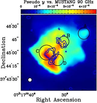
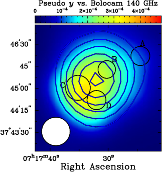
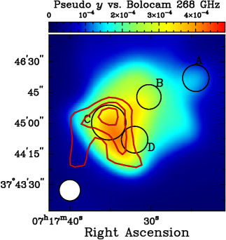
Figure 5.— Contours showing the SZE decrement (increment) for microwave observations below (above) $\sim$218 GHz. Each observation is overlaid on the X-ray pseudo Compton-$y$ map smoothed to the resolution of the instrument (FWHM depicted in the lower left corner of each panel). The subcluster components identified by Ma et al. (2009) are labelled as in Figure 1. Left: MUSTANG observation with point sources subtracted, overlaid on a 10^′′ FWHM smoothed map. Decrement contours are overlaid in blue at the 3$\sigma$, 4$\sigma$, 5$\sigma$, and 6$\sigma$ levels. Note that the MUSTANG data overlaid are filtered with the instrument’s transfer function, while the background image is simply smoothed to 10^′′. Middle: decrement contours from the processed Bolocam 140 GHz data are overlaid in blue at 5$\sigma$, 10$\sigma$, 15$\sigma$, 20$\sigma$, and 25$\sigma$ on the 58^′′ FWHM smoothed pseudo Compton-$y$ map. We note that the data are significantly shifted toward subcluster B, which would be boosted by the kSZE by $\sim 34\%$ assuming the optical velocity along the line of sight, $v_{\mbox{\tiny B}}\approx 3200$ km s^-1 (Ma et al. 2009), is equal to the gas proper velocity. Right: increment contours from the processed Bolocam 268 GHz observation, overlaid in red at 3$\sigma$, 4$\sigma$, and 5$\sigma$ on the 31^′′ FWHM smoothed pseudo Compton-$y$ map. The SZE increment favors the massive component C, which would be boosted by the kSZE up to 10% assuming the optically determined velocity along the line-of-sight, $v_{\mbox{\tiny C}}\approx-700$ km s^-1 (Ma et al. 2009). The total SZE from subcluster B would be suppressed up to $\sim 68\%$ by the kSZE of this high velocity component.

Figure 5 shows the significance contours from each of our SZE observations, overlaid on the X-ray pseudo Compton-$y$ map smoothed to the resolution of each instrument. Qualitatively, the maps at 90 and 140 GHz agree with the X-ray-derived pseudo Compton-$y$ maps. There are two small-scale pressure peaks that are co-spatial with the MUSTANG detections of pressure substructure, and the 140 GHz data and the two-dimensional model (“the tSZE template”) broadly agree. However, there are two main discrepancies: the MUSTANG data show significant levels of substructure – particularly near B – not predicted by the template, and the Bolocam 140 GHz data are shifted $\sim 20^{\prime\prime}$ toward subcluster B. This shift is significant and cannot be explained by pointing offsets; including the $5^{\prime\prime}$ intrinsic uncertainty in the CSO pointing, the Bolocam centroid is determined to $8^{\prime\prime}$ precision.

Looking at the 268 GHz Bolocam data (Figure 5, right), we see a more profound disagreement than that seen in the observations of the SZE decrement. The SZE increment from subcluster C clearly dominates the data, while no flux from B is apparent at $\rm S/N>1$. While the lack of agreement between the MUSTANG 90 GHz detection of subcluster B and the non-detection at 268 GHz could be explained by filtering effects and the lower sensitivity in the 268 GHz Bolocam data, we note that the discrepancy between the Bolocam decrement and increment data cannot be explained by the effects of signal filtering due to the atmospheric noise subtraction. The focal plane geometry, scan pattern, and atmospheric noise subtraction are identical in the Bolocam observations at both frequencies, and the effects of signal filtering are relatively mild and approximately the same at both frequencies. While the noise level is much higher in the 268 GHz observation than that in the 140 GHz observation, it is also clear from the SZE observations alone that flux is missing from component B at 268 GHz, while B is significantly brighter at 140 GHz than the X-ray data indicate it should be.

Table 1Properties of SZE features observed by MUSTANG in MACS J0717.5+3745.

Region	Peak Location (J2000)		Peak $I_{90}$	Peak $y$	Integrated $Y$	Temperature
	R.A.	Dec.	($\mu$Jy bm-1)		$(10^{-12})$	(keV)
NW	07:17:30.68	+37:45:38.1	$-169\pm 37$	$7.7\times 10^{-5}$	$0.99\pm 0.2$	12.8${}^{+2.1}_{-1.6}$
NW src sub			$-164\pm 37$	$7.5\times 10^{-5}$	$0.98\pm 0.2$
NW src+relic sub			$-163\pm 36$	$7.5\times 10^{-5}$	$0.98\pm 0.2$
SE	07:17:33.95	+37:44:49.4	$-188\pm 30$	$9.0\times 10^{-5}$	$2.37\pm 0.3$	34.0${}^{+11}_{-7.9}$
SE src sub			$-207\pm 33$	$9.9\times 10^{-5}$	$2.40\pm 0.2$
SE src+relic sub			$-206\pm 34$	$9.8\times 10^{-5}$	$2.40\pm 0.2$

The properties of the SZE features observed by MUSTANG in MACS J0717.5+3745 are summarized in Table 1. In this table we provide the coordinates and integrated fluxes of the SZE features in the MUSTANG observation. For these, we use the primary MUSTANG map (Figure 2, upper panel), the map with the foreground emission removed (“NW/SE src sub”; Figure 2, lower panel), and a map with all radio sources removed based on upper limits to their fluxes extrapolated from lower frequency radio observations (“NW/SE src+relic sub”; see the discussion below). For the two main SZE features, called the southeast (SE) and northwest (NW) features, we provide estimates of the flux density from the raw map, from the map with the foreground radio source removed, and from the map with the foreground detected source and sources detected at lower frequencies and extrapolated conservatively to 90 GHz removed. We note that our flux density estimates are consistent for all three maps, indicating that the results are robust to radio source contamination.

Table 2 reports the integrated Compton $\mbox{$Y_{\mbox{\tiny tSZE}}$}=\int y\,d\Omega$ computed from model fits of the Arnaud et al. (2010) pressure profile to the 31 GHz CARMA/SZA and 140 GHz Bolocam data. We find that, taken together, the flux in the NW and SE features, as sampled by MUSTANG’s measurements (Table 1), account for $\sim 2\%$ of $Y_{\mbox{\tiny tSZE}}$ on large scales.

We describe below how we quantitatively compare the tSZE template to our SZE observations. For both MUSTANG and Bolocam the pseudo Compton-$y$ maps were first scaled to each instrument’s observing frequency using the relativistic corrections of Itoh et al. (1998) and assuming the temperatures shown in Figure 3. Next, the maps were smoothed with the corresponding PSFs of each instrument, and then filtered to account for the signal attenuation in each instrument’s data processing pipeline.

4.2.1 Modelling the tSZE in the MUSTANG Data

Table 2Large Scale Thermal SZE properties of MACS J0717.5+3745

Instrument	Frequency	Centroid (J2000)		$Y_{500}$
	(GHz)	R.A.	Dec.	$(10^{-10})$
SZA	31	07:17:30.4	+37:45:25.9	$2.04^{+0.20}_{-0.17}$
Bolocam	140	07:17:31.9	+37:45:20.5	$2.44^{+0.50}_{-0.44}$

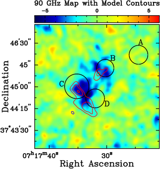
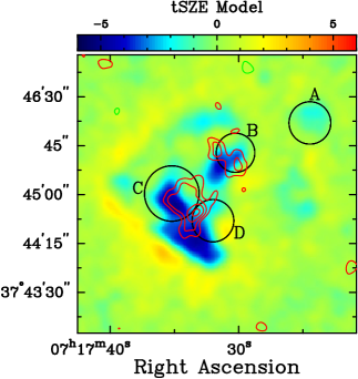
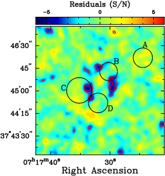
Figure 6.— Left: MUSTANG map with foreground radio source subtracted (as in the lower panel of Figure 2). The contours from the processed pseudo Compton-$y$ model overlaid in red at the -102, -136, -170 $\,\mu$Jy beam^-1level. Middle: Pseudo Compton-$y$ tSZE template processed through the MUSTANG pipeline (corresponding to the contours from the left panel). Contours from MUSTANG map with foreground radio source subtracted are overlaid at 3$\sigma$, 4$\sigma$, 5$\sigma$, and 6$\sigma$, as in the lower panel of Figure 2. Right: Residuals in the MUSTANG data after subtraction of the pseudo Compton-$y$ map and radio point source model from the time ordered data (i.e. the scans used in map-making). Contours are 3$\sigma$ and 4$\sigma$. The point source is cleanly modelled and subtracted, while the X-ray pseudo Compton-$y$ map leaves significant ($>4\sigma$) residual flux on small scales, potentially due to filtering effects in the model (e.g., discontinuities at the temperature region boundaries), the limited X-ray temperature resolution in our $k_{\mbox{\tiny B}}$$T_{\mbox{\tiny e}}$ map, or the complicated line-of-sight structure of the cluster. See text for details.

We fit the radio source in the MUSTANG observation and subtract the cluster template as follows. First, we fit the emission from the foreground elliptical galaxy (detected at $\rm S/N\approx 13.7$) with an elliptical Gaussian. Accounting for our transfer function, the fitted elliptical Gaussian is broadened to $14.4^{\prime\prime}\times 16.1^{\prime\prime}$ FWHM. The cluster template is held fixed, and both the foreground elliptical galaxy and tSZE template were subtracted to produce the maps of the residuals shown in Figure 6.

We also subtract the extended radio feature and compact sources extrapolated from 610 MHz GMRT and 1.4 and 5 GHz VLA data, using a constant power law extrapolation ($\alpha=-1.25$ for the extended feature, and $\alpha=-0.7$ for the compact radio sources). Included with this extrapolation was the detected foreground source. Where associations can be made with FIRST (White et al. 1997), NVSS (Condon et al. 1998), OVRO/BIMA (Coble et al. 2007), or our CARMA/SZA data, we use the measured flux densities to help constrain the spectral index of the source. We also tested subtraction of the extended radio feature using $\alpha=-1.4$. In both cases, the extrapolated sources had a negligible impact. Our spectral extrapolation should place a conservative upper limit on the radio source flux densities at 90 GHz. Synchrotron sources, in general, show steeper spectra at higher frequencies due to radiative losses (e.g., Carilli et al. 1991; Cotton et al. 2009, and references therein). For the inferred $\sim 3~{}\rm\mu G$ magnetic field of the extended halo/relic component (Bonafede et al. 2009), the radiative lifetime of the electrons giving rise to emission at 90 GHz is $\sim 28$ Myr. If this population is older, then the spectrum is likely to be steeper than we have assumed. Recently, Marriage et al. (2011b) measured a steepening on average of radio source spectra above 20 GHz. We find that the contribution from the detected and undetected, extrapolated radio sources has a negligible impact on SZE flux measured at 90 GHz in these MUSTANG maps (see Table 1).

After subtraction, we find a 4$\sigma$ residual flux decrement associated with the interactions of subclusters C and D, located between the strong lensing peaks. This southeast peak (SE) is likely due to the shock-heated gas produced in their merger, as indicated by the X-ray data and supported by the presence of extended radio emission to the north. Restricting our X-ray spectral extraction to the region selected by MUSTANG at 3$\sigma$, containing $\approx 3000$ photon counts, we re-fit the X-ray data and find a temperature $\mbox{$T_{\mbox{\tiny e}}$}=34^{+11}_{-7.4}$ keV (see Table 1), up from $\mbox{$T_{\mbox{\tiny e}}$}=24.1^{+7.1}_{-3.5}$ keV for the contour binned map. If we further restrict our X-ray spectral extraction to the region selected by the residuals in the right-hand panel of Figure 6, we find that we cannot place meaningful constraints on its temperature, despite having $\approx 1200$ X-ray photon counts. This is presumably due to the temperature in that region being above Chandra’s energy range. Since the tSZE is linear with temperature, such a high temperature would increase the expected signal over that in the pseudo Compton-$y$ map by $\sim 40\%$ from this region, and would account entirely for the tSZE residual we found.

We also find residual flux south of subcluster B. This residual is of similar significance as the residual near subclusters C and D. Extracting $\approx 1000$ photon counts from the Chandra data for the region selected by this residual, we find a temperature $\mbox{$T_{\mbox{\tiny e}}$}=14.2^{+3.6}_{-3.2}$ keV. This is within the errorbars for the entire region selected by MUSTANG (see Table 1), while the region’s X-ray surface brightness is much lower than that within region B. We therefore interpret the residual south of region B to be largely an artifact of the subtraction of the pseudo Compton-$y$ template. While the X-ray information aids the interpretation of our high-resolution SZE data, the residual substructure could be due to a number of systematics, discussed below.

Foremost, the binning in the temperature maps produces large discontinuities from region to region. When high pass filtered, this can introduce a ringing effect in the model image (see middle panel of Figure 6). This seems to be the case for the region just to the south of subcluster B. A small, 3$\sigma$ feature appears to be boosted by the positive ringing of an otherwise negative template. Improvements to the modelling and generation of pseudo Compton-$y$ templates will be explored in a future work including relaxed clusters with deeper X-ray data. We note that the X-ray temperature constraints in our $k_{\mbox{\tiny B}}$$T_{\mbox{\tiny e}}$ map come at the cost of reduced resolution in the resulting tSZE template. Many of the temperature bins are $\sim 1~{}\rm arcmin^{2}$ in area, while the resolution of the MUSTANG map is 13^′′. Therefore, some of the larger temperature excursions due to shock heating on small scales could be missing from our X-ray $k_{\mbox{\tiny B}}$$T_{\mbox{\tiny e}}$ map.

Errors in the X-ray derived temperatures as high as $\sim 25\%$ shown in Figure 4 give rise to two additional sources of uncertainty in the tSZE template. The dominant one is simply that pressure scales linearly with temperature, while the additional error due to using the wrong temperature when computing the relativistic correction to the tSZE at 90 GHz anticorrelates with temperature and is on the $\approx-3\%$ level for $\Delta\mbox{$T_{\mbox{\tiny e}}$}/\mbox{$T_{\mbox{\tiny e}}$}\sim+0.25$. Additional sources of possible systematic error that could lead to discrepancies between the X-ray prediction and SZE measurements are clumping and temperature substructure (discussed in §4.1) and the breakdown of the assumption that the effective electron depth $\ell$ is constant (see Equation 3).

4.2.2 Modelling the tSZE in the Bolocam Data

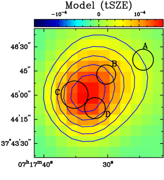
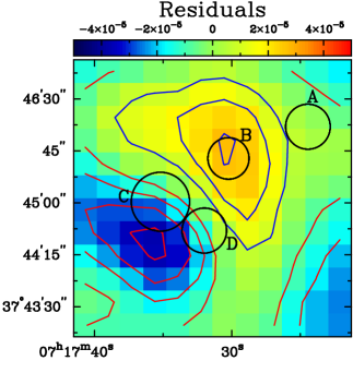
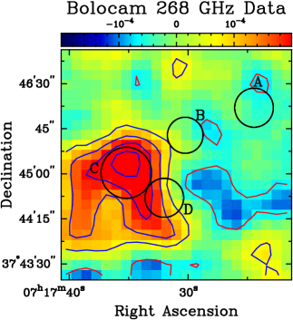
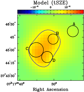
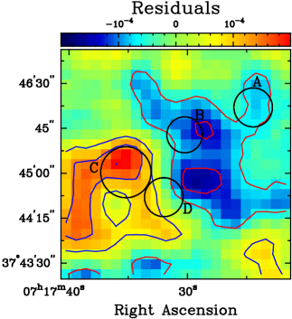
Figure 7.— Bolocam map, processed tSZE template (model), and residuals. Upper panels are for the 140 GHz data, and lower panels are the corresponding plots for the 268 GHz data. Upper Left: Bolocam 140 GHz map, smoothed with a 60^′′ FWHM Gaussian. Contours are overlaid at 3$\sigma$ intervals. Upper Middle: Pseudo Compton-$y$ (tSZE) model at 140 GHz, processed through the same pipeline as the data, so that the filtering effects are the same for the model and data. The normalization was allowed to vary to find the best-fit value for the 140 GHz dataset. Contours are overlaid at 3$\sigma$ intervals. Upper Right: Bolocam 140 GHz residuals after the best-fit pseudo Compton-$y$ model is removed. Contours are overlaid at 1$\sigma$ intervals. Note the color scale was changed to enhance residuals. Lower Left: Bolocam 268 GHz map smoothed with a 30^′′ FWHM Gaussian. Contours are overlaid at 1$\sigma$ intervals. Lower Middle: Same as upper middle, but for the 268 GHz data. Contours are overlaid at 1$\sigma$ intervals. Lower Right: Same as upper right, but for the 268 GHz data. Contours are overlaid at 1$\sigma$ intervals. Note the color scale is unchanged for the 268 GHz plots due to the higher noise level.

For Bolocam we fit the filtered pseudo Compton-$y$ map to our SZE data using a least-squares method and allowing only the normalization of the map to float. In performing the least squares fit we weight the map pixels under the assumption that the map noise covariance is diagonal, as in Sayers et al. (2011). However, since the diagonal noise covariance assumption is not strictly correct, we estimate our derived parameter uncertainties and fit quality via simulation using 1000 statistically-independent noise realizations, as described in more detail in Sayers et al. (2011). We note that by performing the fits in this manner, our parameter uncertainties do not rely on our assumption that the noise covariance is diagonal.

Due to limitations in the extent of the pseudo Compton-$y$ maps, which require accurate temperature determination from X-ray data, the fit was restricted to the inner $4^{\prime}\times 4^{\prime}$ region of our Bolocam data. We find best-fit normalizations of $1.043\pm 0.092$ and $0.839\pm 0.503$ at 140 and 268 GHz, indicating that the pseudo Compton-$y$ maps are consistent with the total integrated SZE signal in the Bolocam data at both observing frequencies. This is expected for the 140 GHz data since the pseudo Compton-$y$ map was normalized so it would have the same $Y_{\mbox{\tiny tSZE}}$ as that found in fits to the Bolocam 140 GHz data. However, the fit quality is actually quite poor at 140 GHz, which we test by computing the value of $\chi^{2}$ to determine the probability to exceed (PTE), which is the probability that we would obtain a fit with a larger value of $\chi^{2}$ due to a random noise fluctuation. For the fit to the 140 GHz data, we find $\chi^{2}/\textrm{DOF}=199/143$, with a $\textrm{PTE}=0.1$%, indicating that the pseudo Compton-$y$ map does not adequately describe our 140 GHz data (note that the fit quality is acceptable for the 268 GHz data, with $\chi^{2}/\textrm{DOF}=624/575$ and $\textrm{PTE}=22$%). Based on the opposite signs of the residuals in units of Compton-$y$ (see Figure 7), we identify a spectral dependence that suggests the presence of a kinetic contribution to the SZE signal, which we show in §5 to improve the fit quality for both data sets.

5. Inferred Peculiar Velocities

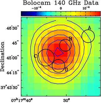
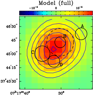
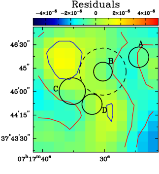
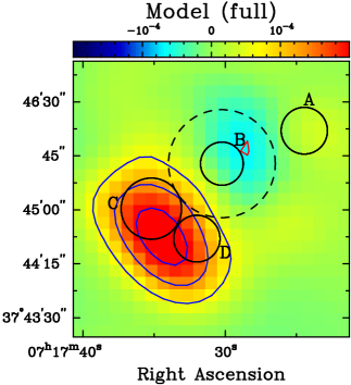
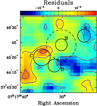
Figure 8.— Bolocam map, processed models (tSZE + kSZE Gaussian), and residuals. Upper panels are for the 140 GHz data, and lower panels are the corresponding plots for the 268 GHz data. Black, dashed circles in middle and right panels show location and size of added 90^′′ FWHM Gaussian model. Upper Left: Bolocam 140 GHz map, smoothed with a 60^′′ FWHM Gaussian. Contours are overlaid at 3$\sigma$ intervals. Upper Middle: Model superposition of the best fit kSZE + pseudo Compton-$y$ template, processed through the same pipeline as the dataset it was used to fit. The normalizations of both models were allowed to vary in order to find the best fit for the dataset. Contours are overlaid at 3$\sigma$ intervals. Upper Right: Bolocam 140 GHz residuals with full model (kSZE + pseudo Compton-$y$) removed. Contours are overlaid at 1$\sigma$ intervals, and the colormap scale was changed to enhance residuals. Lower Left: Bolocam 268 GHz map smoothed with a 30^′′ FWHM Gaussian. Contours are overlaid at 1$\sigma$ intervals. Lower Middle: Pseudo Compton-$y$ (tSZE) model at 268 GHz, processed through the same pipeline as the data, so that the filtering effects are the same for the model and data. The normalizations of both models were freely varied. Contours are overlaid at 1$\sigma$ intervals. Lower Right: Bolocam 268 GHz residuals with full model (kSZE + pseudo Compton-$y$) removed. Contours are overlaid at 1$\sigma$ intervals. Note the color scale is unchanged for the 268 GHz plots.

The residuals of the tSZE template fit, shown in Figure 7, indicate the reason for the poor fit quality of our tSZE template to the Bolocam 140 and 268 GHz data. With the best-fit normalization given in §4.2.2, the pseudo Compton-$y$ map clearly under-predicts the 140 GHz signal near component B and over-predicts the signal near components C and D. Although the 268 GHz data are noisier, the opposite is true; for those data, the pseudo Compton-$y$ map over-predicts the 268 GHz signal near component B and under-predicts the signal near components C and D. Motivated by these results, along with the known, large velocity of the subcluster B, we consider the kSZE as a possible explanation of the opposite discrepancies between our 140 and 268 GHz data and the pseudo Compton-$y$ map. The intensity of the kSZE (Birkinshaw 1999) is

$$\Delta\mbox{$I_{\mbox{\tiny kSZE}}$}=-I_{0}\tau_{e}\,\frac{v_{z}}{c}\frac{x^{4}e^{x}}{(e^{x}-1)^{2}}[1+\delta_{\mbox{\tiny kSZE}}(\mbox{$T_{\mbox{\tiny e}}$},x,v_{z})],$$ (5)

where $v_{z}$ is the line-of-sight proper velocity (positive for a subcluster receding from the observer), $\tau_{e}=\int\mbox{$n_{\mbox{\tiny e}}$}\mbox{$\sigma_{\mbox{\tiny T}}$}d\ell$ is the electron depth, $x\equiv h\nu/(\mbox{$k_{\mbox{\tiny B}}$}\mbox{$T_{\mbox{\tiny CMB}}$})$ is the dimensionless frequency, and $\delta_{\mbox{\tiny kSZE}}(\mbox{$T_{\mbox{\tiny e}}$},x,v_{z})$ is a small relativistic correction which we compute according to Nozawa et al. (2006). It can be seen from Equation 2 that under the assumption of constant temperature along the line-of-sight, $\tau_{e}\propto y/\mbox{$T_{\mbox{\tiny e}}$}$. For fixed Compton-$y$, the kSZE will be suppressed at higher temperature.

Since we lack precise knowledge of the shape of the possible kSZE signal sourced by component B, we chose to describe it using a Gaussian profile with a 90^′′ FWHM. We then re-fit our 140 GHz data with a model consisting of the pseudo Compton-$y$ map and the Gaussian source centered on component B, allowing the normalization of each component to vary. The inclusion of this Gaussian clump significantly improves the fit quality ($\chi^{2}/\textrm{DOF}=153/142$ and $\textrm{PTE}=24$%), indicating both that this Gaussian clump is justified statistically and that the co-added model is adequate to describe our data. Jointly fit with the Gaussian clump, the normalization for the pseudo Compton-$y$ map fit to the 140 GHz data is $0.768\pm 0.084$, indicating the electron depth $\ell\sim 0.8$ Mpc (see §4.1). We then fit the same Gaussian model to our 268 GHz data, allowing the normalizations of it and of the pseudo Compton-$y$ map to float. For this fit, the normalization for the tSZE template fit to the 268 GHz data is $1.78\pm 0.68$. We again find that including the Gaussian clump improves the fit quality ($\chi^{2}/\textrm{DOF}=593/574$ and $\textrm{PTE}=50$%). The combined models and residuals are shown in Figure 8.

Table 3X-ray temperature and inferred peculiar velocities

Subcluster	$k_{\mbox{\tiny B}}$$T_{\mbox{\tiny e}}$	$\Delta v$	$S_{\mbox{\tiny 140~{}\rm GHz}}$	$S_{\mbox{\tiny 268~{}\rm GHz}}$	$v_{\mbox{\tiny\rm z}}$
Name	(keV)	(km s-1)	(mJy)	(mJy)	(km s-1)
B (model)	13.7${}^{+2.1}_{-1.6}$	$+3238^{+252}_{-242}$	$-19.5\pm 2.0$	$1.9\pm 5.8$	$+3600^{+3440}_{-2160}$
B (nonpar)			$-17.0\pm 2.1$	$-0.5\pm 7.5$	$+4640^{+6720}_{-3360}$
C (model)	24.1${}^{+7.1}_{-3.5}$	$-733^{+486}_{-478}$	$-14.7\pm 1.6$	$18.5\pm 7.5$	$-3720^{+2960}_{-2480}$
C (nonpar)			$-13.0\pm 1.7$	$17.7\pm 8.5$	$-4120^{+3760}_{-2880}$

Using the results of our model fits to compute flux density, we attempt to fit for a tSZE+kSZE spectrum that can adequately describe subcluster B, the highest velocity member of MACS J0717.5+3745. For comparison, we also fit the spectrum of subcluster C, since it is the most massive component, it has a lower known optical velocity ($\approx-700$ km s^-1), and it is detected at 5$\sigma$ in the 268 GHz data. We also verify our model-dependent results using non-parametric, model-independent estimates of the flux densities from the deconvolved images for each of these regions. For all combinations of methods and regions, we use the integrated flux densities obtained from within 1^′ diameter apertures centered on subcluster B or C. The values are listed in Table 3. We perform a grid search over the possible velocities, temperatures, and values for $Y_{\mbox{\tiny tSZE}}$ in each region. We include the X-ray $k_{\mbox{\tiny B}}$$T_{\mbox{\tiny e}}$ constraints for each region when we compute $\chi^{2}$ for each combined, relativistically-corrected thermal + kinetic SZE spectrum that can describe our measurements.

Our joint constraints on velocity and $Y_{\mbox{\tiny tSZE}}$ for these regions, using both the model dependent and non-parametric fluxes, are shown in Figure 9. Also shown in Figure 9 are the 1 and 2$\sigma$ constraints on each parameter when marginalizing over the other (the $\Delta\chi^{2}<1$ and $\Delta\chi^{2}<4$ regions for projection to the axis of interest). Note that the values of $Y_{\mbox{\tiny tSZE}}$ and peculiar velocity are anticorrelated, leading to a wide possible range for both when fitting only two bands of SZE data. Marginalizing over $Y_{\mbox{\tiny tSZE}}$ for each region, the median and 1$\sigma$ errors on velocity are reported in Table 3. The inferred kSZE+tSZE spectra are plotted in Figure 10. We find that the probability of $v_{z}\leq 0$ is 2.1% for the fits to the model-derived flux density for subcluster B, and 3.4% for the non-parametric flux density estimates. For subcluster C, we find the probability of $v_{z}\geq 0$ is 15.7% for the model flux density estimates, and 19.3% for the nonparametric flux density estimates. All of our peculiar velocity estimates agree with the Ma et al. (2009) optical estimates to within 1$\sigma$.

The possibility of using the CARMA/SZA 31 GHz data, which should be relatively insensitive to the kSZE contribution, to better constrain the tSZE component was considered. However, the synthesized beam in our CARMA/SZA 31 GHz observations was over 2^′, while we are fitting components at the arcminute scale, and would thus make the results difficult to compare directly.

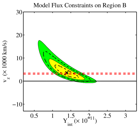
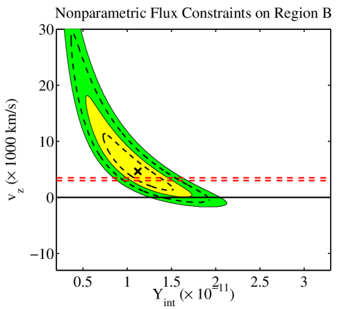
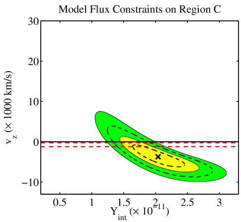
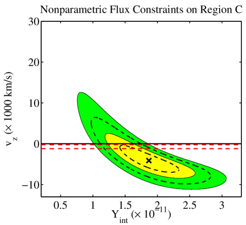
Figure 9.— SZE constraints on peculiar velocity and $Y_{\mbox{\tiny tSZE}}$ from the Bolocam 140 and 268 GHz data. Each subcluster was assumed to be isothermal, and X-ray spectroscopic contraints were used to marginalize over temperature. Yellow regions contain $\Delta\chi^{2}<2.3$ (68.3% confidence interval on both parameters), and green regions contain $\Delta\chi^{2}<6.17$ (95.4% confidence interval on both parameters). Black dashed lines enclose $\Delta\chi^{2}<1$ and $\Delta\chi^{2}<4$, the 1 and 2$\sigma$ confidence intervals on the parameters taken individually (i.e. marginalizing over the other parameter). An ‘X’ marks the minimum in $\chi^{2}$. The horizontal red dashed lines mark 1$\sigma$ constraints from the Ma et al. (2009) optical spectroscopic velocity measurements. Upper Left: Constraints on peculiar velocity and $Y_{\mbox{\tiny tSZE}}$ using the fluxes measured from the model fits within a 1^′ diameter region centered on subcluster B. Upper Right: Same as upper left, but using the nonparametric flux measurements. Lower Left: Same as upper left, but for subcluster C. Lower Right: Same as lower left, but using the nonparametric flux measurements.

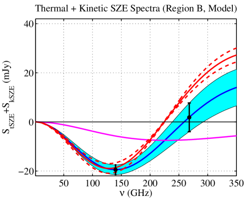
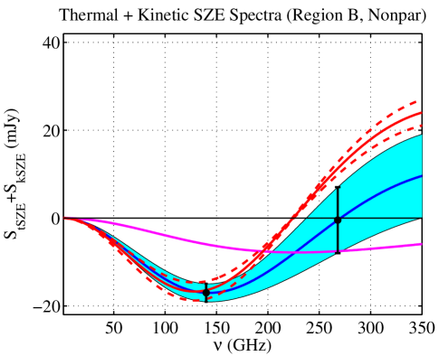
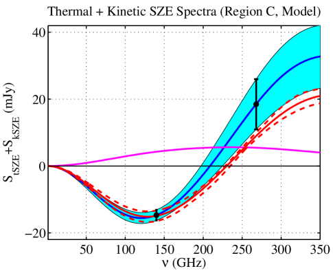
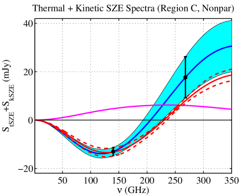
Figure 10.— Upper Left: Spectral sum of tSZE and kSZE flux densities for subcluster B, using the measurements obtained from the model fits to the Bolocam 140 and 268 GHz data (black points with error bars). The best fit combined SZE spectrum is plotted as a solid blue line, with 1$\sigma$ errors displayed as the cyan region. SZE spectral fits were obtained through a joint likelihood analysis for the Bolocam data including Chandra $k_{\mbox{\tiny B}}$$T_{\mbox{\tiny e}}$ likelihood constraints. The kSZE contribution for the best fit velocity in Table 3 is plotted in magenta (solid line). A pure tSZE spectrum to the data is plotted in red (solid line, with dashed lines indicating the 68.3% confidence interval). Spectra with $v_{z}\leq 0$ have a probability of 2.1% given these data. Upper Right: Same as upper left, but using the flux density measured directly (nonparametrically) at 140 and 268 GHz from the deconvolved data. Spectra with $v_{z}\leq 0$ have a probability of 3.4% given these data. Lower Left: Same as upper right, but for subcluster C. Spectra with $v_{z}\geq 0$ have a probability of 15.7% given these data. Lower Right: Same as upper right, but for subcluster C. Spectra with $v_{z}\geq 0$ have a probability of 19.3% given these data.

Our measurements of the SZE spectra using 140 and 268 GHz Bolocam data are sensitive to several possible systematic errors, which we describe here. Errors due to the relative flux calibration were included in our flux estimates. Since the regions used in the analysis are 60^′′ in diameter, and the pointing information in each dataset is accurate to better than 5^′′, this result cannot be explained by pointing errors. We also consider possible contamination from dusty, star forming “submillimeter” galaxies (SMGs) which have been included in our noise model in a statistical sense, though bright and/or lensed SMGs could bias our measurements, particularly at higher frequencies. The direction of the submillimeter contamination is key: deviation from a purely thermal SZE spectrum from B requires a negative flux density at both 140 and 268 GHz, so (positive) contamination from SMGs would cause us to underestimate the kSZE signal rather than overestimate it. The inferred large, negative proper velocity of subcluster C could potentially be affected by a SMG, but is nevertheless consistent with the optical velocity to better than 1$\sigma$. Importantly, submm Herschel maps show no indication of contamination at a significant level in either region. The extended radio emission near C – too faint at 90 GHz to be seen in the much more sensitive MUSTANG observations – cannot explain the kSZE component of subcluster C, nor can compact radio sources, constrained by the MUSTANG observation to be $\lesssim 90$ $\,\mu$Jy beam^-1 at 90 GHz. Finally, temperature substructure due to clumping, merger activity, or the remnant core in B could increase the variance in our estimates, but since there is no way to constrain the size of this clumping effect with these data we defer to future work.

6. Conclusions

High resolution, multi-wavelength observations of the SZE are now beginning to offer measurements that are truly complementary to X-ray and optical studies of the complicated dynamics in galaxy clusters. Here we have presented sensitive, sub-arcminute measurements from MUSTANG at 90 GHz and from Bolocam at 140 and 268 GHz. We compared these with lower resolution SZE observations obtained with CARMA/SZA at 31 GHz. We also compared our SZE observations to the detailed lensing, optical dynamics, radio, and our own results using Chandra X-ray data to build a two-dimensional template for modelling the tSZE in this cluster.

The primary feature in MUSTANG’s high-pass-filtered, high-resolution view of the cluster seems to be associated with the merger activity between two subcluster components (C and D in the Figure 1). This feature is also strong in Bolocam’s 268 GHz, 31^′′-resolution map of MACS J0717.5+3745, and is associated with the hottest gas, which approaches $\sim 30$ keV in spectral fits to the Chandra X-ray data from that region of the sky. The feature is bracketed by non-thermal, extended emission from the relativistic gas seen in GMRT 610 MHz and VLA 1.4–5 GHz observations, providing further supporting evidence for a merger scenario and a multi-phase intra-cluster medium. The MUSTANG observation also reveals significant features at subcluster B which could include contributions from high temperature or density substructures. MUSTANG’s measurements account for $\sim 2\%$ of the integrated pressure on large scales, as measured in the Bolocam 140 GHz and CARMA/SZA 31 GHz data.

Using the X-ray data to constrain the integrated line-of-sight pressure, and normalizing it to the large scale SZE observations, we constructed a two-dimensional template for the tSZE in this cluster. The use of the bulk SZE measurements for normalization allows us to convert the X-ray pseudo-pressure map into units of Compton-$y$, and yields a value for the effective depth of the ICM that is consistent with the cluster’s scale ($\sim 1~{}\rm Mpc$). While assumptions about the line-of-sight structure must be made and the model is imperfect, a simple spherical model for this unvirialized structure is clearly insufficient. The detailed comparison of these tSZE templates with the SZE data allows us to infer the presence of pressure substructure not constrained by X-ray observations alone. Further, we presented for the first time subtraction of compact radio source contamination from the MUSTANG time-ordered data used in making our maps.

By subtracting the radio source contamination from the MUSTANG data, and the tSZE template from both, our observations revealed residuals indicating that the X-ray-derived tSZE template provides a poor fit that can only qualitatively describe the data. For the MUSTANG data, the residuals indicate significant pressure or temperature substructure not seen in the X-ray (e.g., out of band hot gas), but could also be due to a number of systematics (e.g., clumping, assumption of a constant line-of-sight depth, temperature substructure, or filtering and data processing effects).

For the Bolocam data, the residual component at subcluster B after subtraction of the template is negative in intensity both below and above the null ($\sim 220$ GHz) in the tSZE spectrum. The residuals are therefore inconsistent with a purely tSZE component—either as an excess or deficit—or any possible compact radio or submillimeter source. Further, considering the high velocity ($\approx 3200$ km s^-1) of subcluster B, we find this residual to be consistent with the kSZE. We note that this measurement is on resolved, subcluster scales, rather than being due to the proper motion of the cluster as a whole.

Using flux densities extracted from our model fits, and marginalizing over the X-ray spectroscopic temperature constraints for the region, we found that the high-velocity subcluster B has a best-fit line-of-sight proper velocity of $3600^{+3440}_{-2160}$ km s^-1. This agrees with the optical velocity estimate for the galaxies associated with the subcluster. While our results depend on assumptions about the line-of-sight temperature structure and the accuracy of the X-ray temperature determination, we find that the probability $v_{z}\leq 0$ given our data is 2.1%. We also fit the SZE spectrum of the most massive subcluster, C. For this, we found $-3720^{+2960}_{-2480}$, with a 15.7% probability a $v_{z}\geq 0$ SZE spectrum can describe the region given our data and assumptions.

We also compared our peculiar velocity estimates with spectral fits using the fluxes measured nonparametrically from the same regions of the maps, and find the probability a $v_{z}\leq 0$ SZE spectrum can describe our data for subcluster B is 3.4%. For region C, the probability is 19.3% that $v_{z}\geq 0$ given our data.

This tantalizing result is among the highest significance indications of non-zero kSZE from an individual galaxy cluster yet (see e.g., Holzapfel et al. 1997; Benson et al. 2003; Mauskopf et al. 2012; Zemcov et al. 2012). Even more exciting is that the kSZE spectral component required is on subcluster scales. Clearly, this cluster will be an interesting target for both detailed modelling of the dynamics and for future SZE studies.

A simple justification for the “slab approximation,” which assumes the temperature is constant along the line-of-sight, is as follows. The expression for X-ray surface brightness is

$$\mbox{$S_{\mbox{\tiny X}}$}=\frac{1}{4\pi(1+z)^{3}}\!\int\!\!\mbox{$n_{\mbox{\tiny e}}$}^{2}\mbox{$\Lambda_{\mbox{\tiny ee}}$}(\mbox{$T_{\mbox{\tiny e}}$},Z)\,d\ell,$$ (1)

where $\mbox{$\Lambda_{\mbox{\tiny ee}}$}(\mbox{$T_{\mbox{\tiny e}}$},Z)$ contains the extra $(1+z)^{-1}$ factor required by cosmological dimming. In the absence of any true line-of-sight information about the cluster, we defer to the standard spherical approximation. Assuming a standard $\beta$ profile for the density,

$$\mbox{$n_{\mbox{\tiny e}}$}(r)=n_{\mbox{\tiny e0}}\left[1+(r/r_{c})^{2}\right]^{-3\beta/2},$$ (2)

then surface brightness as a function of sky angle $\theta$ is (e.g., Sarazin 1988; Reese et al. 2002; LaRoque et al. 2006)

$$\mbox{$S_{\mbox{\tiny X}}$}(\theta)=S_{\mbox{\tiny X0}}\left[1+(\theta/\theta_{c})^{2}\right]^{(1-6\beta)/2}.$$ (3)

For pressure—allowing for the slope $\beta_{P}$ to be different from the density profile’s slope $\beta$ (i.e. non-isothermal ICM)—we have

$$\mbox{$P_{\mbox{\scriptsize e}}$}(r)=P_{\mbox{\tiny e0}}\left[1+(r/r_{c})^{2}\right]^{-3\beta_{P}/2}.$$ (4)

Using $y=\mbox{$\sigma_{\mbox{\tiny T}}$}/(\mbox{$m_{\mbox{\tiny e}}c^{2}$})\int\mbox{$P_{\mbox{\scriptsize e}}$}d\ell$, Compton-$y$ as a function of sky angle $\theta$ is (see e.g., Reese et al. 2002; LaRoque et al. 2006)

$$y(\theta)=y_{\mbox{\tiny 0}}\left[1+(\theta/\theta_{c})^{2}\right]^{(1-3\beta_{P})/2}.$$ (5)

Taking $\beta=0.7$ (e.g., LaRoque et al. 2006) as the average density slope and $\beta_{P}=0.86$ for the average pressure slope (see e.g., Plagge et al. 2010; Marriage et al. 2011a; Reese et al. 2012), the ratio of $y(\theta)$ to $\sqrt{\mbox{$S_{\mbox{\tiny X}}$}(\theta)}$ is now proportional to $\left[1+(\theta/\theta_{c})^{2}\right]$ raised to a power of $(1-3\beta_{P})/2-(1-6\beta)/4=3(\beta-\beta_{P})/2+1/4=0.01\approx 0$. The assumption that the slope is 0 (i.e. the slab approximation is valid) is within the error bars reported on the average slopes $\beta$ and $\beta_{P}$, and prevents the resulting pseudo Compton-$y$ map from becoming unbounded at the map edges.

We emphasize that this result does not imply pressure is constant along the line of sight, but rather that the average ratio of Compton-$y$ to $\sqrt{\mbox{$S_{\mbox{\tiny X}}$}}$ is approximately constant. The underlying pressure and density profiles are assumed, on average, to be described by their respective $\beta$-model parameterizations ($\beta=0.7$ and $\beta_{P}=0.86$). If we were to assume $\beta=2/3$ for the density profile instead, this would yield a $\beta$-model taper to the power of -0.14. Both of these choices of $\beta$, along with $\beta_{P}=0.86$, are consistent with a polytropic index of 1.2–1.3, which are in turn consistent with values reported in recent studies (Bautz et al. 2009; Capelo et al. 2012).

References

- Arnaud et al. (2010) Arnaud, M., Pratt, G. W., Piffaretti, R., Böhringer, H., Croston, J. H., & Pointecouteau, E. 2010, A&A, 517, A92
- Bautz et al. (2009) Bautz, M. W., Miller, E. D., Sanders, J. S., Arnaud, K. A., Mushotzky, R. F., Porter, F. S., Hayashida, K., Henry, J. P., Hughes, J. P., Kawaharada, M., Makashima, K., Sato, M., & Tamura, T. 2009, PASJ, 61, 1117
- Benson et al. (2003) Benson, B. A., Church, S. E., Ade, P. A. R., Bock, J. J., Ganga, K. M., Hinderks, J. R., Mauskopf, P. D., Philhour, B., Runyan, M. C., & Thompson, K. L. 2003, ApJ, 592, 674
- Birkinshaw (1999) Birkinshaw, M. 1999, Phys. Rep., 310, 97
- Bonafede et al. (2009) Bonafede, A., Feretti, L., Giovannini, G., Govoni, F., Murgia, M., Taylor, G. B., Ebeling, H., Allen, S., Gentile, G., & Pihlström, Y. 2009, A&A, 503, 707
- Capelo et al. (2012) Capelo, P. R., Coppi, P. S., & Natarajan, P. 2012, MNRAS, 2719
- Carilli et al. (1991) Carilli, C. L., Perley, R. A., Dreher, J. W., & Leahy, J. P. 1991, ApJ, 383, 554
- Carlstrom et al. (2002) Carlstrom, J. E., Holder, G. P., & Reese, E. D. 2002, ARA&A, 40, 643
- Cavagnolo et al. (2009) Cavagnolo, K. W., Donahue, M., Voit, G. M., & Sun, M. 2009, ApJS, 182, 12
- Clarke & Ensslin (2006) Clarke, T. E. & Ensslin, T. 2006, Astronomische Nachrichten, 327, 553
- Coble et al. (2007) Coble, K., Bonamente, M., Carlstrom, J. E., Dawson, K., Hasler, N., Holzapfel, W., Joy, M., La Roque, S., Marrone, D. P., & Reese, E. D. 2007, AJ, 134, 897
- Condon et al. (1998) Condon, J. J., Cotton, W. D., Greisen, E. W., Yin, Q. F., Perley, R. A., Taylor, G. B., & Broderick, J. J. 1998, AJ, 115, 1693
- Cotton et al. (2009) Cotton, W. D., Mason, B. S., Dicker, S. R., Korngut, P. M., Devlin, M. J., Aquirre, J., Benford, D. J., Moseley, S. H., Staguhn, J. G., Irwin, K. D., & Ade, P. 2009, ApJ, 701, 1872
- Dicker et al. (2008) Dicker, S. R., Korngut, P. M., Mason, B. S., Ade, P. A. R., Aguirre, J., Ames, T. J., Benford, D. J., Chen, T. C., Chervenak, J. A., Cotton, W. D., Devlin, M. J., Figueroa-Feliciano, E., Irwin, K. D., Maher, S., Mello, M., Moseley, S. H., Tally, D. J., Tucker, C., & White, S. D. 2008, in Society of Photo-Optical Instrumentation Engineers (SPIE) Conference Series, Vol. 7020, Society of Photo-Optical Instrumentation Engineers (SPIE) Conference Series
- Ebeling et al. (2004) Ebeling, H., Barrett, E., & Donovan, D. 2004, ApJ, 609, L49
- Ebeling et al. (2007) Ebeling, H., Barrett, E., Donovan, D., Ma, C.-J., Edge, A. C., & van Speybroeck, L. 2007, ApJ, 661, L33
- Ebeling et al. (2001) Ebeling, H., Edge, A. C., & Henry, J. P. 2001, ApJ, 553, 668
- Edge et al. (2003) Edge, A. C., Ebeling, H., Bremer, M., Röttgering, H., van Haarlem, M. P., Rengelink, R., & Courtney, N. J. D. 2003, MNRAS, 339, 913
- Haig et al. (2004) Haig, D. J., Ade, P. A. R., Aguirre, J. E., Bock, J. J., Edgington, S. F., Enoch, M. L., Glenn, J., Goldin, A., Golwala, S., Heng, K., Laurent, G., Maloney, P. R., Mauskopf, P. D., Rossinot, P., Sayers, J., Stover, P., & Tucker, C. 2004, in Society of Photo-Optical Instrumentation Engineers (SPIE) Conference Series, Vol. 5498, Society of Photo-Optical Instrumentation Engineers (SPIE) Conference Series, ed. C. M. Bradford, P. A. R. Ade, J. E. Aguirre, J. J. Bock, M. Dragovan, L. Duband, L. Earle, J. Glenn, H. Matsuhara, B. J. Naylor, H. T. Nguyen, M. Yun, & J. Zmuidzinas, 78–94
- Holzapfel et al. (1997) Holzapfel, W. L., Ade, P. A. R., Church, S. E., Mauskopf, P. D., Rephaeli, Y., Wilbanks, T. M., & Lange, A. E. 1997, ApJ, 481, 35
- Itoh et al. (1998) Itoh, N., Kohyama, Y., & Nozawa, S. 1998, ApJ, 502, 7
- Itoh & Nozawa (2004) Itoh, N. & Nozawa, S. 2004, A&A, 417, 827
- Kitayama et al. (2004) Kitayama, T., Komatsu, E., Ota, N., Kuwabara, T., Suto, Y., Yoshikawa, K., Hattori, M., & Matsuo, H. 2004, PASJ, 56, 17
- Komatsu et al. (2009) Komatsu, E., Dunkley, J., Nolta, M. R., Bennett, C. L., Gold, B., Hinshaw, G., Jarosik, N., Larson, D., Limon, M., Page, L., Spergel, D. N., Halpern, M., Hill, R. S., Kogut, A., Meyer, S. S., Tucker, G. S., Weiland, J. L., Wollack, E., & Wright, E. L. 2009, ApJS, 180, 330
- Komatsu et al. (2011) Komatsu, E., Smith, K. M., Dunkley, J., Bennett, C. L., Gold, B., Hinshaw, G., Jarosik, N., Larson, D., Nolta, M. R., Page, L., Spergel, D. N., Halpern, M., Hill, R. S., Kogut, A., Limon, M., Meyer, S. S., Odegard, N., Tucker, G. S., Weiland, J. L., Wollack, E., & Wright, E. L. 2011, ApJS, 192, 18
- Korngut et al. (2011) Korngut, P. M., Dicker, S. R., Reese, E. D., Mason, B. S., Devlin, M. J., Mroczkowski, T., Sarazin, C. L., Sun, M., & Sievers, J. 2011, ApJ, 734, 10
- LaRoque et al. (2006) LaRoque, S. J., Bonamente, M., Carlstrom, J. E., Joy, M. K., Nagai, D., Reese, E. D., & Dawson, K. S. 2006, ApJ, 652, 917
- Limousin et al. (2012) Limousin, M., Ebeling, H., Richard, J., Swinbank, A. M., Smith, G. P., Jauzac, M., Rodionov, S., Ma, C.-J., Smail, I., Edge, A. C., Jullo, E., & Kneib, J.-P. 2012, A&A, 544, A71
- Ma et al. (2009) Ma, C.-J., Ebeling, H., & Barrett, E. 2009, ApJ, 693, L56
- Ma et al. (2008) Ma, C.-J., Ebeling, H., Donovan, D., & Barrett, E. 2008, ApJ, 684, 160
- Markevitch & Vikhlinin (2007) Markevitch, M. & Vikhlinin, A. 2007, Phys. Rep., 443, 1
- Marriage et al. (2011a) Marriage, T. A., Acquaviva, V., Ade, P. A. R., Aguirre, P., Amiri, M., Appel, J. W., Barrientos, L. F., Battistelli, E. S., Bond, J. R., Brown, B., Burger, B., Chervenak, J., Das, S., Devlin, M. J., Dicker, S. R., Bertrand Doriese, W., Dunkley, J., Dünner, R., Essinger-Hileman, T., Fisher, R. P., Fowler, J. W., Hajian, A., Halpern, M., Hasselfield, M., Hernández-Monteagudo, C., Hilton, G. C., Hilton, M., Hincks, A. D., Hlozek, R., Huffenberger, K. M., Handel Hughes, D., Hughes, J. P., Infante, L., Irwin, K. D., Baptiste Juin, J., Kaul, M., Klein, J., Kosowsky, A., Lau, J. M., Limon, M., Lin, Y.-T., Lupton, R. H., Marsden, D., Martocci, K., Mauskopf, P., Menanteau, F., Moodley, K., Moseley, H., Netterfield, C. B., Niemack, M. D., Nolta, M. R., Page, L. A., Parker, L., Partridge, B., Quintana, H., Reese, E. D., Reid, B., Sehgal, N., Sherwin, B. D., Sievers, J., Spergel, D. N., Staggs, S. T., Swetz, D. S., Switzer, E. R., Thornton, R., Trac, H., Tucker, C., Warne, R., Wilson, G., Wollack, E., & Zhao, Y. 2011a, ApJ, 737, 61
- Marriage et al. (2011b) Marriage, T. A., Baptiste Juin, J., Lin, Y.-T., Marsden, D., Nolta, M. R., Partridge, B., Ade, P. A. R., Aguirre, P., Amiri, M., Appel, J. W., Barrientos, L. F., Battistelli, E. S., Bond, J. R., Brown, B., Burger, B., Chervenak, J., Das, S., Devlin, M. J., Dicker, S. R., Bertrand Doriese, W., Dunkley, J., Dünner, R., Essinger-Hileman, T., Fisher, R. P., Fowler, J. W., Hajian, A., Halpern, M., Hasselfield, M., Hernández-Monteagudo, C., Hilton, G. C., Hilton, M., Hincks, A. D., Hlozek, R., Huffenberger, K. M., Handel Hughes, D., Hughes, J. P., Infante, L., Irwin, K. D., Kaul, M., Klein, J., Kosowsky, A., Lau, J. M., Limon, M., Lupton, R. H., Martocci, K., Mauskopf, P., Menanteau, F., Moodley, K., Moseley, H., Netterfield, C. B., Niemack, M. D., Page, L. A., Parker, L., Quintana, H., Reid, B., Sehgal, N., Sherwin, B. D., Sievers, J., Spergel, D. N., Staggs, S. T., Swetz, D. S., Switzer, E. R., Thornton, R., Trac, H., Tucker, C., Warne, R., Wilson, G., Wollack, E., & Zhao, Y. 2011b, ApJ, 731, 100
- Mason et al. (2010) Mason, B. S., Dicker, S. R., Korngut, P. M., Devlin, M. J., Cotton, W. D., Koch, P. M., Molnar, S. M., Sievers, J., Aguirre, J. E., Benford, D., Staguhn, J. G., Moseley, H., Irwin, K. D., & Ade, P. 2010, ApJ, 716, 739
- Maughan et al. (2008) Maughan, B. J., Jones, C., Forman, W., & Van Speybroeck, L. 2008, ApJS, 174, 117
- Mauskopf et al. (2012) Mauskopf, P. D., Horner, P. F., Aguirre, J., Bock, J. J., Egami, E., Glenn, J., Golwala, S. R., Laurent, G., Nguyen, H. T., & Sayers, J. 2012, MNRAS, 421, 224
- McNamara et al. (2005) McNamara, B. R., Nulsen, P. E. J., Wise, M. W., Rafferty, D. A., Carilli, C., Sarazin, C. L., & Blanton, E. L. 2005, Nature, 433, 45
- Muchovej et al. (2007) Muchovej, S., Mroczkowski, T., Carlstrom, J. E., Cartwright, J., Greer, C., Hennessy, R., Loh, M., Pryke, C., Reddall, B., Runyan, M., Sharp, M., Hawkins, D., Lamb, J. W., Woody, D., Joy, M., Leitch, E. M., & Miller, A. D. 2007, ApJ, 663, 708
- Nord et al. (2009) Nord, M., Basu, K., Pacaud, F., Ade, P. A. R., Bender, A. N., Benson, B. A., Bertoldi, F., Cho, H., Chon, G., Clarke, J., Dobbs, M., Ferrusca, D., Halverson, N. W., Holzapfel, W. L., Horellou, C., Johansson, D., Kennedy, J., Kermish, Z., Kneissl, R., Lanting, T., Lee, A. T., Lueker, M., Mehl, J., Menten, K. M., Plagge, T., Reichardt, C. L., Richards, P. L., Schaaf, R., Schwan, D., Spieler, H., Tucker, C., Weiss, A., & Zahn, O. 2009, A&A, 506, 623
- Nozawa et al. (2006) Nozawa, S., Itoh, N., Suda, Y., & Ohhata, Y. 2006, Nuovo Cimento B Serie, 121, 487
- Plagge et al. (2010) Plagge, T., Benson, B. A., Ade, P. A. R., Aird, K. A., Bleem, L. E., Carlstrom, J. E., Chang, C. L., Cho, H.-M., Crawford, T. M., Crites, A. T., de Haan, T., Dobbs, M. A., George, E. M., Hall, N. R., Halverson, N. W., Holder, G. P., Holzapfel, W. L., Hrubes, J. D., Joy, M., Keisler, R., Knox, L., Lee, A. T., Leitch, E. M., Lueker, M., Marrone, D., McMahon, J. J., Mehl, J., Meyer, S. S., Mohr, J. J., Montroy, T. E., Padin, S., Pryke, C., Reichardt, C. L., Ruhl, J. E., Schaffer, K. K., Shaw, L., Shirokoff, E., Spieler, H. G., Stalder, B., Staniszewski, Z., Stark, A. A., Vanderlinde, K., Vieira, J. D., Williamson, R., & Zahn, O. 2010, ApJ, 716, 1118
- Plagge et al. (2012) Plagge, T. J., Marrone, D. P., Abdulla, Z., Bonamente, M., Carlstrom, J. E., Gralla, M., Greer, C. H., Joy, M., Lamb, J. W., Leitch, E. M., Mantz, A., Muchovej, S., & Woody, D. 2012, ArXiv e-prints
- Reese et al. (2002) Reese, E. D., Carlstrom, J. E., Joy, M., Mohr, J. J., Grego, L., & Holzapfel, W. L. 2002, ApJ, 581, 53
- Reese et al. (2010) Reese, E. D., Kawahara, H., Kitayama, T., Ota, N., Sasaki, S., & Suto, Y. 2010, ApJ, 721, 653
- Reese et al. (2012) Reese, E. D., Mroczkowski, T., Menanteau, F., Hilton, M., Sievers, J., Aguirre, P., Appel, J. W., Baker, A. J., Bond, J. R., Das, S., Devlin, M. J., Dicker, S. R., Dünner, R., Essinger-Hileman, T., Fowler, J. W., Hajian, A., Halpern, M., Hasselfield, M., Hill, J. C., Hincks, A. D., Huffenberger, K. M., Hughes, J. P., Irwin, K. D., Klein, J., Kosowsky, A., Lin, Y.-T., Marriage, T. A., Marsden, D., Moodley, K., Niemack, M. D., Nolta, M. R., Page, L. A., Parker, L., Partridge, B., Rojas, F., Sehgal, N., Sifón, C., Spergel, D. N., Staggs, S. T., Swetz, D. S., Switzer, E. R., Thornton, R., Trac, H., & Wollack, E. J. 2012, ApJ, 751, 12
- Rudy (1987) Rudy, D. J. 1987, PhD thesis, California Inst. of Tech., Pasadena.
- Russell et al. (2010) Russell, H. R., Sanders, J. S., Fabian, A. C., Baum, S. A., Donahue, M., Edge, A. C., McNamara, B. R., & O’Dea, C. P. 2010, MNRAS, 406, 1721
- Sanders (2006) Sanders, J. S. 2006, MNRAS, 371, 829
- Sarazin (1988) Sarazin, C. L. 1988, X-ray emission from clusters of galaxies (Cambridge Astrophysics Series, Cambridge: Cambridge University Press, 1988)
- Sarazin (2005) Sarazin, C. L. 2005, in X-Ray and Radio Connections, ed. L. O. Sjouwerman & K. K. Dyer
- Sayers et al. (2012) Sayers, J., Czakon, N. G., & Golwala, S. R. 2012, ApJ, 744, 169
- Sayers et al. (2011) Sayers, J., Golwala, S. R., Ameglio, S., & Pierpaoli, E. 2011, ApJ, 728, 39
- Sunyaev & Zel’dovich (1972) Sunyaev, R. A. & Zel’dovich, Y. B. 1972, Comments Astrophys. Space Phys., 4, 173
- van Weeren et al. (2009) van Weeren, R. J., Röttgering, H. J. A., Brüggen, M., & Cohen, A. 2009, A&A, 505, 991
- White et al. (1997) White, R. L., Becker, R. H., Helfand, D. J., & Gregg, M. D. 1997, ApJ, 475, 479
- Zemcov et al. (2012) Zemcov, M., Aguirre, J., Bock, J., Bradford, C. M., Czakon, N., Glenn, J., Golwala, S. R., Lupu, R., Maloney, P., Mauskopf, P., Million, E., Murphy, E. J., Naylor, B., Nguyen, H., Rosenman, M., Sayers, J., Scott, K. S., & Zmuidzinas, J. 2012, ApJ, 749, 114
- Zitrin et al. (2009) Zitrin, A., Broadhurst, T., Rephaeli, Y., & Sadeh, S. 2009, ApJ, 707, L102