Non-Abelian $SU(2)$ gauge fields through density-wave order and strain in graphene

Abstract

Spatially varying strain patterns can qualitatively alter the electronic properties of graphene, acting as effective valley-dependent magnetic fields and giving rise to pseudo-Landau-level (PLL) quantization Novoselov et al. (2005). Here, we show that the strain-induced magnetic field is one component of an $SU(2)$ non-Abelian gauge field within the low-energy theory of graphene, and identify the other two components as period-3 charge-density waves. We show that these density-waves, if spatially varied, give rise to PLL quantization. We also argue that strain-induced magnetic fields can induce density-wave order in graphene, thus dynamically gapping out the lowest PLL; moreover, the ordering should generically be accompanied by dislocations. We discuss experimental signatures of these effects.

The discovery of graphene Novoselov et al. (2005)—a carbon monolayer with low-energy electronic properties governed by the Dirac equation Castro Neto et al. (2009)—has stimulated enormous interest in condensed matter systems having Dirac quasiparticles. Although other systems supporting Dirac quasiparticles have subsequently been discovered (e.g., the surface bands of topological insulators Qi and Zhang (2011); Hasan and Kane (2010)), graphene is uniquely tunable through lattice deformations and strains, being a soft two-dimensional membrane Castro Neto et al. (2009). Strains alter the electronic structure of graphene by modulating the hopping amplitudes between neighboring lattice sites. A striking example of the electronic consequences of strain is that certain spatially varying patterns of deformation can mimic the effects of a pseudo-“magnetic field” that has opposite signs in the vicinity of the two Dirac points (which we shall refer to as the valleys K and $\textbf{K}^{\prime}$ Guinea et al. (2010)). Such pseudo-magnetic fields, on the order of $300$ Tesla, were recently demonstrated in pioneering experiments Levy and al. (2010) on nanoscale graphene bubbles; more recently, effective fields of order $60$ Tesla were realized by artificially designing a lattice of carbon-monoxide molecules on copper Gomes et al. (2012). At these fields, each valley is deep in the quantum Hall regime, so that its electronic structure consists of well-spaced pseudo-Landau levels (PLLs). Because the PLLs are highly degenerate, one expects correlation effects to be strong within them; indeed, recent works have shown that, in the presence of interactions, partially-filled PLLs are unstable to forming ordered states such as valley ferromagnets, spin-Hall phases and triplet superconductors Ghaemi et al. ; Pesin and Abanin .

In the present work we show that the strain-induced, valley-dependent magnetic field is one component of a non-Abelian $SU(2)$ gauge field within the low-energy theory of graphene. We identify the other two generators of this $SU(2)$ gauge field as period-3 charge-density waves (3CDWs) (Fig. 1) that mix the $\mathbf{K}$ and $\mathbf{K}^{\prime}$ valleys. We show that these charge-density waves act as gauge potentials: when their amplitude is constant, they move the Dirac cones [Fig. 2(B)]; but when their amplitude is spatially varied, they can give rise to Landau-level quantization, as shown in Fig. 3. Although methods for realizing non-Abelian $SU(2)$ gauge fields had previously been proposed in ultracold atomic settings Osterloh et al. (2005); Lin et al. (2011); Goldman et al. (2009) and in twisted bilayer graphene San-Jose et al. , such fields have yet to be experimentally realized in condensed matter. The present work suggests an alternative approach, which might be easier to implement, e.g., in molecular graphene Gomes et al. (2012).

Having established the $SU(2)$ gauge structure, we turn to the effects of the 3CDW patterns on the PLL structure induced by strain. We find that, although these perturbations do not open up gaps in unstrained graphene, they do gap out the lowest (i.e., zero-energy) PLL. On general grounds, then, we expect these gaps, and the corresponding 3CDW patterns, to be dynamically generated by electron-electron or electron-phonon interactions whenever graphene is strained, as they would reduce the ground-state energy. (The relation between different mass gaps and the corresponding ordered states was previously explored, for unstrained graphene, in Refs. Ghaemi et al. (2010); Ghaemi and Ryu (2012); Ryu et al. (2009).)

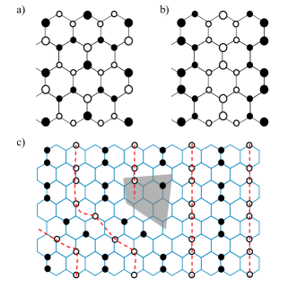
Figure 1: $SU(2)$ gauge potentials [i.e., charge-density-wave (3CDW) patterns] and their defects. Panels (a) and (b) show the patterns corresponding to $\zeta_{x,1}$ and $\zeta_{y,2}$ respectively (see Table 1 for definitions); the other two patterns are related to these by translation. Black (white) circles denote excess positive (negative) charge; larger circles correspond to greater excess charge. Panel (c) sketches a dislocation in the 3CDW pattern; the dislocation core is marked in gray. Dashed red lines trace the crests of the 3CDW pattern.

After discussing the 3CDW patterns, we turn to their defects (i.e., dislocations), and show that these defects are entwined with the ordering in a distinctive way, owing to the valley-dependence of the pseudo-magnetic field. In contrast with the case of a regular field, for a strain-induced field a uniform 3CDW perturbation does not mix the spatially coincident Landau orbitals in the two valleys, as these are counter-propagating. However, a 3CDW perturbation with a defect at the origin can mix the valleys and open up a gap. Thus, in experimental geometries such as that of Ref. Levy and al. (2010), the defects as well as the order are likely to be dynamically generated.

Model. In the absence of interactions, the tight-binding Hamiltonian of strained graphene reads

$$H_{0}=\sum_{\mathbf{r}_{i}}\sum_{a=1,2,3}(t+\delta t_{a}(\mathbf{r}_{i}))(a^{\dagger}(\mathbf{r}_{i})b(\mathbf{r}_{i}+\mbox{\boldmath$\delta$}_{a})+h.c.),$$ (1)

where $\delta t_{a}(\mathbf{r}_{i})$ is the strain-induced variation of the nearest neighbour hopping amplitude between the $A$-sublattice site at $\mathbf{r}_{i}$ and the $B$-sublattice site at $\mathbf{r}_{i}+\mbox{\boldmath$\delta$}_{a}$ of the bipartite honeycomb lattice Castro Neto et al. (2009). The vectors $\mbox{\boldmath$\delta$}_{a}$ connect any $A$-sublattice atom to its three $B$-sublattice nearest neighbors. In the absence of strain, the low-energy excitations correspond to linearly dispersing states close to the two Dirac points at momenta $\pm{\bf K}$ with ${\bf K}=(4\pi/3\sqrt{3}a_{0}){\bf e_{x}}$, $a_{0}$ being the carbon-carbon bond length Castro Neto et al. (2009). Near the Dirac points $\mathbf{K}$ and $\mathbf{K}^{\prime}$ the wavefunctions of such states can be written as four-component spinors $\Psi\equiv(\psi_{A,\mathbf{K}},\psi_{B,\mathbf{K}},\psi_{A,\mathbf{K}^{\prime}},\psi_{B,\mathbf{K}^{\prime}})$ where the first index denotes the component of the wavefunction on the $A(B)$ sublattice of the honeycomb unit cell, and the second index denotes the component of the state that is associated with the $\mathbf{K}$ ($\mathbf{K}^{\prime}$) valley. The low energy effective Hamiltonian close to the Dirac points reads as:

$$\mathcal{H}_{0}=v_{F}\left[\hat{p}_{x}\Gamma_{x}+\hat{p}_{y}\Gamma_{y}\right]$$ (2)

where $\Gamma_{x}=\tau_{3}\sigma_{1}$, $\Gamma_{y}=\tau_{0}\sigma_{2}$, $v_{F}$ is the Fermi velocity, and the $\sigma$ and $\tau$ operators are Pauli matrices acting on sublattice and valley indices respectively. We have not included the physical spin index as it does not affect our analysis, provided that the spin-orbit coupling is negligible.

There are three terms in the low-energy theory (i.e., “charges”) that commute with the Hamiltonian (2): $Q_{1}\equiv-\tau_{2}\sigma_{2},\quad Q_{2}\equiv\tau_{1}\sigma_{2},\quad Q_{3}\equiv\tau_{3}\sigma_{0}$. These realize an $SU(2)$ pseudo-spin algebra $\left[Q_{i},Q_{j}\right]=2{i}\epsilon_{ijk}Q_{j}$. We also define the electromagnetic $U(1)$ charge $Q_{0}\equiv\tau_{0}\sigma_{0}$ (i.e., the identity operator), which commutes with the other charges. We can minimally couple $\mathcal{H}_{0}$ to the gauge potentials associated with these charges, thus arriving at the Hamiltonian:

$$\mathcal{H}=v_{F}\left[\Gamma_{x}\left(\hat{p}_{x}-\sum_{i=0}^{3}A_{x}^{i}Q_{i}\right)+\Gamma_{y}\left(\hat{p}_{y}-\sum_{i=0}^{3}A_{y}^{i}Q_{i}\right)\right].$$ (3)

We turn to the microscopic origins of the $SU(2)$ gauge potentials, $\zeta_{\mu,i}\equiv\Gamma_{\mu}Q_{i}$, where $\mu=x,y$ and $i=1,2,3$. Of these, $\zeta_{\mu,3}$ comprise the familiar strain-induced vector potential. Strain generates a gauge field given by $A_{x}^{0}+iA_{y}^{3}=\sum_{a=1,2,3}\delta t_{a}(\textbf{r})e^{\pm i\textbf{K}\cdot\mbox{\boldmath$\delta$}_{a}}$ near the Dirac points $\pm\mathbf{K}$. Note that $\sum_{a=1,2,3}\delta t_{a}(\textbf{r})e^{\pm i\textbf{K}\cdot\mbox{\boldmath$\delta$}_{a}}$ is complex because the nearest-neighbor hoppings are not symmetric under inversion. The real part of the strain gauge field $A_{x}^{0}$ is the same in both valleys and therefore couples to $Q_{0}$; it can be gauged away assuming time-reversal symmetry holds. On the other hand, the imaginary part $iA_{y}^{3}$ has opposite sign in the two valleys and couples to $Q_{3}$ leading to the valley-dependent magnetic fields realized in the experiments of Ref. Levy and al. (2010).

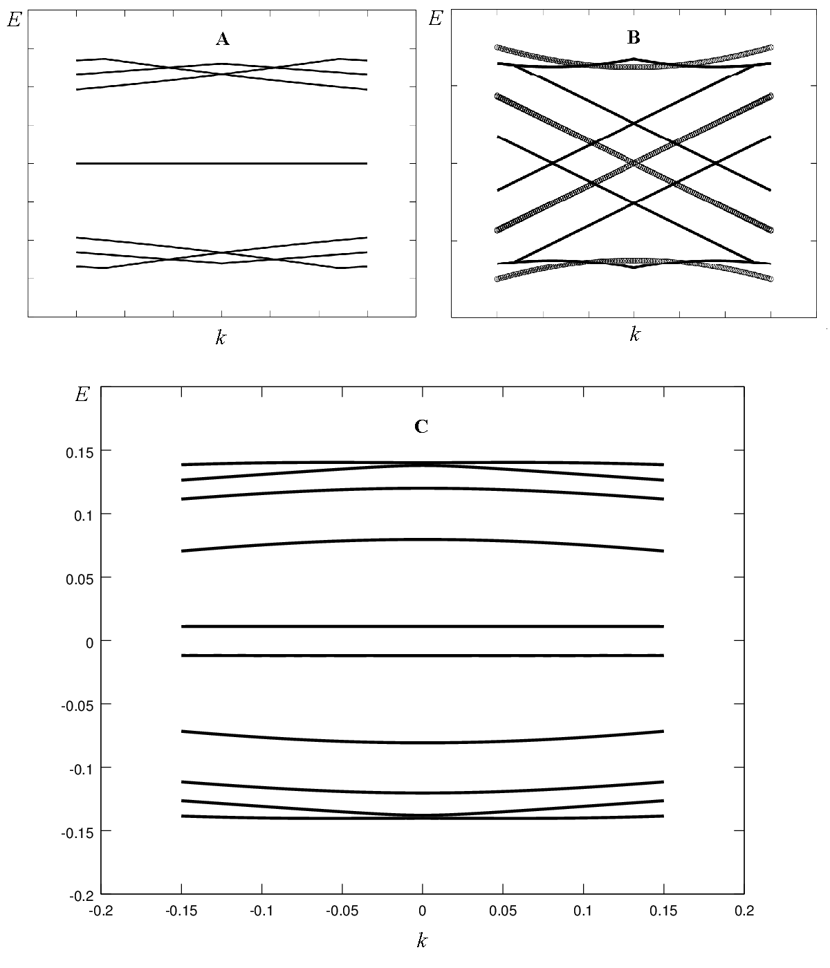
Figure 2: (A) The band structure in the presence of strain, calculated for a 100-site thick graphene nanoribbon with zigzag edges, showing pseudo-Landau levels (PLLs). All energies are computed in terms of the unperturbed hopping matrix element; in the presence of strain, the hopping along one of the three directions increases linearly from $t$ to $1.9t$ across the sample. Note that the zero-energy level is in fact fourfold degenerate, including both two zero-energy PLLs and two modes localized on zigzag edges. (B) The location of the Dirac cones in the absence of strain, both with the perturbation $\zeta_{x,i}$ (thin solid line) and without it (thick line). As noted in the main text, constant gauge potentials are expected to shift the Dirac cones. (C) The band structure in the presence of both strain and the perturbation $\zeta_{x,i}$. Note that the fourfold-degenerate zero-energy mode is completely split, with the two more widely separated levels corresponding to the lowest PLL. (This was checked by explicitly computing the wavefunctions.)

The four remaining gauge potentials (see Table 1) originate, as we shall now see, as 3CDWs. That they should be charge density waves can be seen as follows: (a) the perturbations mix the valleys, and must therefore involve spatial modulations that enlarge the unit cell; (b) they do not mix the sublattices (i.e., they are proportional either to $\sigma_{3}$ or to $\sigma_{0}$), and can therefore include only on-site charge offsets and intra-sublattice (e.g., next-nearest neighbor) hopping. Two simple perturbations satisfying both criteria are charge modulations of wavevector $\mathbf{G}$ (where $\mathbf{G}\equiv\mathbf{K}-\mathbf{K}^{\prime}$ is a vector connecting the two Dirac points), which realize $\tau_{1}$ and $\tau_{2}$ respectively:

$$\tau_{1}\leftrightarrow\cos(\mathbf{G\cdot r}),\quad\tau_{2}\leftrightarrow\sin(\mathbf{G\cdot r}).$$ (4)

The gauge potentials $\zeta_{x,i}$ are realized when the density waves on $A$ and $B$ sublattices are $\pi$ out of phase, whereas the potentials $\zeta_{y,i}$ are realized when the density waves on the $A$ and $B$ sublattices are in phase. Fig. 1 shows the two corresponding density-wave arrangements, which are listed in Table 1.

Term	Low-energy	LPLL	Microscopic
$\zeta_{x,1}$	$\tau_{1}\sigma_{3}$	$\tau_{1}$	$\cos(\mathbf{G\cdot r})\cos\left[\pi(y/a_{0}+\frac{1}{4})\right]$
$\zeta_{x,2}$	$\tau_{2}\sigma_{3}$	$\tau_{2}$	$\sin(\mathbf{G\cdot r})\cos\left[\pi(y/a_{0}+\frac{1}{4})\right]$
$\zeta_{y,1}$	$\tau_{2}\sigma_{0}$	$\tau_{2}$	$\sin(\mathbf{G\cdot r})$
$\zeta_{y,2}$	$\tau_{1}\sigma_{0}$	$\tau_{1}$	$\cos(\mathbf{G\cdot r})$

Table 1: Density-wave-based gauge potentials in graphene. This table lists the microscopic and low-energy forms of the perturbations, as well as the forms after projection onto the lowest pseudo-Landau level (LPLL).

Numerical band structure calculations on nano-ribbons including these terms are shown in Figs. 2 and 3; as one can see, the $\zeta$’s do not open up gaps in the absence of strain, but do shift the Dirac points in momentum space, as a vector potential is expected to do. Moreover, if the coefficient of $\zeta_{y,2}$, say, is varied linearly with $x$ (cf. the Landau gauge description of a uniform magnetic field), it gives rise to PLL quantization as shown in Fig. 3. We have thus established that these terms can be regarded, together with the strain-induced gauge potentials, as enabling the realization of a general $SU(2)$ gauge field.

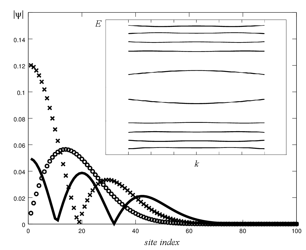
Figure 3: Pseudo-Landau levels (PLLs) generated by the $SU(2)$ pseudo-gauge potential $A^{2}_{x}Q_{2}=BQ_{2}y$ on a 100-site nanoribbon with zigzag edges. The value of $Q_{2}$ varies linearly from zero at one end of the ribbon to $0.74t$ at the other end. The main panel shows wavefunctions in the first, second, and third distinct PLL, calculated on a 100-site nanoribbon with zigzag edges. The inset shows the overall level structure (cf. Fig. 2A, for the case of regular strain), demonstrating that the PLLs are indeed flat for momenta near the Dirac cone.

Strain-induced PLLs and their mass gaps. The pseudospin $SU(2)$ symmetry (at low energies) allowed us to treat the strain and 3CDWs on the same footing in the preceding discussion. We now break this symmetry by considering the PLL structure created by a strain pattern inducing a uniform pseudo-magnetic field. The eigenstates of $\mathcal{H}$ then fall into PLLs at energies $E_{n}\sim\sqrt{n}$, and in particular there is a PLL at zero energy in each valley Castro Neto et al. (2009), which we term the LPLL. While the LPLL shares some features with the zero-energy Landau levels induced by a real magnetic field, it is distinct in two essential ways, as follows. (1) In contrast with the case of a real magnetic field (in which the two lowest Landau level wavefunctions in the two valleys are located on opposite sublattices), the LPLL wavefunctions in both valleys are located entirely on the $A$ sublattice Ghaemi et al. . (2) The wavefunctions in the LPLL in the $\mathbf{K}$($\mathbf{K}^{\prime}$) valleys have the four-component form $\Psi^{\mathbf{K}}_{0,m}=(\phi_{0,m},0,0,0)$ and $\Psi^{\mathbf{K}^{\prime}}_{0,m}=(0,0,\phi_{0,m}^{*},0)$, respectively, where $\phi_{0,m}$ is the $m$th Landau orbital in the lowest (nonrelativistic) Landau level (see below). [By contrast, in the case of a real magnetic field, the second of these would be $\Psi^{\mathbf{K}^{\prime}}_{0,m}=(0,0,0,\phi_{0,m})$.] Thus, in a pseudo-magnetic field, the PLL orbitals are counter-propagating, whereas in a real magnetic field they are co-propagating. Consequently, for a real magnetic field, the valley index can be regarded as a mere flavor degree of freedom, and a uniform valley-mixing perturbation mixes the Landau orbitals in the two valleys. However, for strained graphene, the valley index should not be interpreted as a flavor index, because the wavefunctions in the two valleys are spatially distinct. As we shall see, this implies that inhomogeneous mass terms (i.e., mass terms with defects) are necessary to gap the LPLL. The precise consequences depend on which gauge in pseudo-vector potentials is simulated by the strain pattern. (This is possible because, while two gauge-equivalent electromagnetic vector potentials are physically identical, different pseudo-vector potentials are physically distinct as they correspond to different patterns of strain.)

Uniform perturbations. We now address point (1) from the previous paragraph, ignoring spatial structure and considering the effects of uniform (i.e., defect-free) 3CDW perturbations precisely at zero momentum (i.e., at the Dirac point). Many of the properties of the LPLL follow from the triviality of its sublattice structure: in particular, one can find the form of any perturbation in the LPLL by projecting it onto the $A$ sublattice. Thus, perturbations within the LPLL are completely described by $2\times 2$ matrices in $\tau$ (i.e., valley) space (Table 1). As a consequence, several perturbations that open up gaps in unstrained graphene, such as an intra-unit-cell charge-density wave ($\sigma_{3}\tau_{0}$) and the Kekulé distortion ($\sigma_{1}\tau_{1}$), are trivial when projected to the LPLL. However, the $SU(2)$ gauge potentials $\zeta_{\mu,i}$ do open up gaps within the LPLL, as they project onto either $\tau_{1}$ or $\tau_{2}$ (Table 1), and can thus mix LPLL orbitals from the $\mathbf{K}$ and $\mathbf{K}^{\prime}$ valleys.

The two further perturbations that split the LPLL are valley polarization, $m_{p}\equiv\tau_{3}\sigma_{0}$, and the Haldane mass Haldane (1988), $m_{H}\equiv\tau_{3}\sigma_{3}$. Within the LPLL, these terms are equivalent; both correspond to $\tau_{3}$, which shifts the energy of one valley with respect to the other. Both terms anticommute with the gauge fields; therefore, within the low-energy theory, it seems that these masses can be continuously deformed into one another. (Thus, the fate of the topologically-protected edge mode associated with $m_{H}$ cannot be addressed within the low-energy theory. Numerical calculations of the band structure in the presence of both $m_{H}$ and $\zeta_{x,i}$ suggest that as $\zeta_{x,i}$ is increased, the edge state drifts away from the Dirac points; it is therefore plausible that $\zeta_{x,i}$ and $m_{H}$ compete away from the Dirac points. We shall revisit this question in future work.)

The perturbations discussed above are likely to be dynamically generated in experiments with neutral graphene (i.e., a half-filled LPLL), as opening up a gap would lower the ground-state energy. The 3CDWs could arise either because of the electron-phonon coupling or the electron-electron coupling; moreover, a spontaneous valley polarization might arise due to electron-electron interactions Ghaemi et al. . Alternatively, one can externally impose these gaps by growing graphene on an appropriately patterned substrate.

Momentum dependence. We now turn to the second distinctive feature of the PLLs [point (2) above] and discuss the role played by the spatial structure of PLL wavefunctions. In order to address this, we shall consider the nature of the 3CDW perturbations on orbitals away from the Dirac point.

We first consider the strain pattern realizing the Landau gauge; here, if the 3CDW amplitude is uniform, the left-valley Landau orbital $\phi_{0,m}(x,y)\propto e^{i\frac{2\pi m}{L}x}e^{-\left(y-\frac{2\pi m}{L}l^{2}\right)^{2}/l^{2}}$ ($l$ being the magnetic length) can hybridize only with the right-valley Landau orbital $\phi^{*}_{0,-m}(x,y)\propto e^{i\frac{2\pi m}{L}x}e^{-\left(y+\frac{2\pi m}{L}l^{2}\right)^{2}/l^{2}}$, due to the conservation of $k_{x}$. Although the overlap between these two states is nonzero, it decreases as $|m|$ is increased, and becomes exponentially small for $ml\gg L$. This decrease of overlap leads to the convexity of the LPLL gap shown in Fig. 2, and implies that the 3CDW gap is an inherently mesoscopic phenomenon. (However, note that all experimental realizations of pseudo-magnetic fields in strained graphene involve mesoscopic systems.)

Point defects. If the strain realizes a symmetric gauge pattern, $\phi_{0,m}(r,\theta)\propto e^{im\theta}r^{m}e^{-r^{2}/l^{2}}$, as in the experiments of Ref. Levy and al. (2010), the consequences are even more striking. Here, the only allowed orbitals have $m\geq 0$, because otherwise $\phi_{0,m}$ is not normalizable. As a result, no uniform perturbation can gap out the $m\neq 0$ orbitals. Thus, in order to open up a gap, it is necessary to consider configurations in which the perturbations have defects, i.e., edge dislocations in the 3CDW case. Within the LPLL, the two independent 3CDW orders are represented by $\tau_{1}$ and $\tau_{2}$ (Table 1). The 3CDW can support edge dislocations [Fig. 1(c)], which take the form of vortex solutions within the LPLL theory:

$$\Delta(r)\left[\tau_{1}\cos(n\theta)+\tau_{2}\sin(n\theta)\right]=\left(\begin{array}[]{cc}0&\Delta(r)e^{in\theta}\\ \Delta(r)e^{-in\theta}&0\end{array}\right)$$ (5)

where $\Delta(r)$ is a function that vanishes at $r=0$ and is constant for $r\gg l_{M}$. Such vortex solutions carry angular momentum, so that they can lead to hybridization of different orbitals in the LPLL:

$$\int d\theta dr\left(\phi^{*}_{0,m},0\right)\Delta(r)\left[\tau_{1}\cos(n\theta)+\tau_{2}\sin(n\theta)\right]\left(\begin{array}[]{c}0\\ \phi^{*}_{0,m^{\prime}}\end{array}\right)$$ (8)

$$\quad\propto\delta_{0,n-m-m^{\prime}}$$ (9)

for vorticity $n$, the Landau orbitals with $m<n$ will be gapped. As a result, a larger vorticity can gap out more Landau orbitals and will thus lead to lower energy (although a larger vorticity might also cost greater electrostatic or elastic energy). In this case, one expects the defects to be dynamically generated along with the 3CDW patterns.

Effects in higher PLLs. We now turn to the effects of the aforementioned perturbations when projected onto higher PLLs. In the higher PLLs, the sublattice structure is not trivial, so that the six masses are distinct perturbations. These perturbations fall into two classes, depending on whether their sublattice component is $\sigma_{0}$ or $\sigma_{3}$. Perturbations of the former class split all the PLLs. For the valley polarization term, this is obvious by inspection: a polarization of the form $\tau_{z}$ moves all the PLLs in the $\mathbf{K}$ up and all those at $\mathbf{K}^{\prime}$ down, thus opening up a gap of size $2\alpha$ between any pair of PLLs. Similarly, degenerate perturbation theory shows that the perturbations $\zeta_{y,i}$ mix $\Psi^{\mathbf{K}}_{n,m}$ and $\Psi^{\mathbf{K}^{\prime}}_{n,m}$ (assuming, for simplicity, that the strain pattern realizes the Landau gauge). By contrast, $m_{H}$ and $\zeta_{x,i}$ do not mix $\Psi^{\mathbf{K}}_{n,m}$ and $\Psi^{\mathbf{K}^{\prime}}_{n,m}$, and thus preserve the double degeneracy of higher PLLs. However, these perturbations do mix $\Psi^{\mathbf{K}}_{n,m}$ and $\Psi^{\mathbf{K}^{\prime}}_{-n,m}$, thus shifting the energy of the $n$th PLL by $\alpha^{2}/(2\Delta_{0}\sqrt{n})$, where $\Delta_{0}$ is the cyclotron energy scale.

These considerations might influence which set of perturbations is in fact dynamically generated. In particular, if one of the nonzero PLLs is half-filled, the favored perturbations are those of the $\sigma_{0}$ class. By contrast, at half-filling of the LPLL (i.e., for neutral graphene), the above argument suggests that the $\sigma_{3}$ class of perturbations is preferred, as these lower the energy of the filled negative-energy PLLs. It is not clear, however, whether this energy saving is outweighed by changes in band structure away from the Dirac points.

Experimental aspects. We close by touching upon various experimental considerations. The 3CDW ordering described here can either be realized spontaneously in the presence of strain, or imposed externally. In the former case, the pattern of ordering can be detected easily via scanning-tunneling microscopy (STM); this technique is commonly used to study stripe ordering, e.g., in high-temperature superconductors (see, e.g., Ref. Howald et al. (2003)). Alternatively, one can study the 3CDW perturbations by externally imposing them. This is easiest to do in the case of engineered systems, such as molecular graphene Gomes et al. (2012), where a 3CDW pattern such as $\zeta_{y,i}$ can be imposed by hand on the triangular network of adsorbate molecules (or, alternatively, for hexagonal optical lattices Soltan-Panahi et al. (2011)). However, it might also be possible to realize it using systems of graphene grown on anisotropic substrates, which favor 3CDW formation.

Acknowledgments. S.G. and P.G. are indebted to Paul Goldbart for helpful discussions. The authors acknowledge support from DOE DE-FG02-07ER46453 (S.G.) and ICMT at UIUC (P.G.).

References

- Novoselov et al. (2005) K. S. Novoselov, A. K. Geim, S. V. Morozov, D. Jiang, M. I. Katsnelson, I. V. Grigorieva, S. V. Dubonos, and A. A. Firsov, Nature, 438, 197 (2005).
- Castro Neto et al. (2009) A. H. Castro Neto, F. Guinea, N. M. R. Peres, K. S. Novoselov, and A. K. Geim, Rev. Mod. Phys., 81, 109 (2009).
- Qi and Zhang (2011) X.-L. Qi and S.-C. Zhang, Rev. Mod. Phys. (2011).
- Hasan and Kane (2010) M. Z. Hasan and C. L. Kane, Rev. Mod. Phys., 82, 3045 (2010).
- Guinea et al. (2010) F. Guinea, M. Katsnelson, and A. Geim, Nat. Phys., 6, 30 (2010).
- Levy and al. (2010) L. Levy and al., Science, 329, 544 (2010).
- Gomes et al. (2012) K. K. Gomes, W. Mar, W. Ko, F. Guinea, and H. C. Manoharan, Nature, 483, 306 (2012).
- (8) P. Ghaemi et al., arXiv:1111.3640.
- (9) D. Pesin and D. Abanin, arXiv:1112.6420.
- Osterloh et al. (2005) K. Osterloh, M. Baig, L. Santos, P. Zoller, and M. Lewenstein, Phys. Rev. Lett., 95, 010403 (2005).
- Lin et al. (2011) Y.-J. Lin, K. Jiménez-García, and I. Spielman, Nature, 471, 83 (2011).
- Goldman et al. (2009) N. Goldman, A. Kubasiak, P. Gaspard, and M. Lewenstein, Phys. Rev. A, 79, 023624 (2009).
- (13) P. San-Jose, J. González, and F. Guinea, ArXiv:1110.2883 (2011).
- Ghaemi et al. (2010) P. Ghaemi, S. Ryu, and D.-H. Lee, Phys. Rev. B, 81, 081403 (2010).
- Ghaemi and Ryu (2012) P. Ghaemi and S. Ryu, Phys. Rev. B, 85, 075111 (2012).
- Ryu et al. (2009) S. Ryu, C. Mudry, C.-Y. Hou, and C. Chamon, Phys. Rev. B, 80, 205319 (2009).
- Haldane (1988) F. Haldane, Phys. Rev. Lett., 61, 2015 (1988).
- Howald et al. (2003) C. Howald, H. Eisaki, N. Kaneko, and A. Kapitulnik, Proc. Nat. Acad. Sci, 100, 9705 (2003).
- Soltan-Panahi et al. (2011) P. Soltan-Panahi, J. Struck, P. Hauke, A. Bick, W. Plenkers, G. Meineke, C. Becker, P. Windpassinger, M. Lewenstein, and K. Sengstock, Nat. Phys., 7, 434 (2011).