The Fortuin-Kasteleyn and Damage Spreading transitions in Random bond Ising lattices
Abstract
The Fortuin-Kasteleyn and heat-bath damage spreading temperatures and are studied on random bond Ising models of dimension two to five and as functions of the ferromagnetic interaction probability ; the conjecture that is tested. It follows from a statement by Nishimori that in any such system exact coordinates can be given for the intersection point between the Fortuin-Kasteleyn transition line and the Nishimori line, . There are no finite size corrections for this intersection point. In dimension three, at the intersection concentration the damage spreading is found to be equal to to within . For the other dimensions however is observed to be systematically a few percent lower than .
pacs:
75.50.Lk, 05.50.+q, 64.60.Cn, 75.40.CxI Introduction
The physics of Ising spin glasses (ISGs) in the ”ordered” regime below the freezing temperature has been intensively investigated for decades; the paramagnetic regime above has attracted less attention. However, in addition to the standard ordering (or freezing) transitions other significant ”critical” temperatures within the paramagnetic regime can be defined operationally and estimated numerically with high precision.
We have studied random-bond Ising models (RBIM) in dimensions two, three, four and five having ferromagnetic near neighbor interactions with probability and antiferromagnetic interactions with probability over the whole range of in the paramagnetic regime. The Hamiltonian is where the sum is taken over all nearest neighbour bonds .
For the discrete interaction distribution the bond values are thus chosen according to
| (1) |
We will set and use when convenient inverse temperatures . The pure Ising model is recovered for and the pure antiferromagnetic model for , while the standard strong disorder bimodal spin glass case corresponds to .
In addition to the standard ferromagnetic and spin glass ordering transitions, on the RBIM phase diagram in the paramagnetic regime other physically significant lines can be operationally defined as functions of . In addition to the Griffiths line () griffiths:69 ; matsuda:08 and the Nishimori line nishimori:81 there is the Fortuin-Kasteleyn (FK) transition line fortuin:72 ; coniglio:80 ; coniglio:91 ; dearcangelis:91 ; cataudella:91 ; zhang:93 and the heat-bath damage spreading transition line derrida:87 ; derrida:89 ; dearcangelis:89 ; campbell:91 . Early large scale relaxation measurements on the ISG in dimension three were interpreted ogielski:85 in terms of a dynamic transition at the Griffiths temperature (i.e. ), with a qualitative change in relaxation behavior of the autocorrelation function from non-exponential to exponential.
It can alternatively be considered that or defines a dynamic transition. At the FK cluster size diverges so the standard cluster flipping algorithms swendsen:87 ; wolff:89 break down. At , the time scale for the ”coupling from the past” equilibration criterion diverges at large propp:96 ; bernard:10 so this criterion similarly breaks down. A priori it seems plausible that the two dynamic breakdowns should occur at similar, if perhaps not identical, temperatures as has been conjectured by a number of authors dearcangelis:91 ; campbell:94 ; yamaguchi:10 .
In the following discussion it is shown that there are universal analytic relations for the intersection point between and the Nishimori line nishimori:81 . With these exact values in hand together with the present accurate numerical damage spreading data a critical test can be made of the conjectured rule . This is shown to be a good approximation, almost exact in dimension three and accurate to a few percent in dimensions two, four and five. However the equality between the temperatures is not a general rule.
II Transition definitions
Nishimori nishimori:81 has shown for the RBIM that, due to extra symmetries of the problem, a number of quantities may be computed exactly when the equality
| (2) |
holds; this condition defines the Nishimori line (NL), a line traversing the entire phase diagram including both paramagnetic and ferromagnetic regimes. In particular on the NL the internal energy of the system per bond (or edge) is
| (3) |
This energy per bond has exactly the value that independent bonds would have at the same temperature. We will see below that indeed on the NL the positions of the satisfied bonds are uncorrelated nishimori:86 ; nishimori and that bond positions remain very close to random over a wide strong disorder regime around . In other words anywhere on the NL the satisfied bonds are uncorrelated on average, so a fortiori the FK active bonds are distributed at random.
The rule for the Fortuin-Kasteleyn (FK) transition line fortuin:72 ; coniglio:80 ; coniglio:91 ; dearcangelis:91 ; cataudella:91 ; zhang:93 , corresponding initially to the pure ferromagnets, is to first select for some particular equilibrium configuration the entire set of ”satisfied” bonds where is positive. These bonds are then decimated at random leaving a fraction of ”active” satisfied bonds. The FK stochastic transition at occurs when the set of active bonds percolates through the lattice. From the way in which the bonds are laid down, in the general case this is correlated bond percolation, as opposed to the standard uncorrelated bond percolation with random bond occupation. Remarkably, for pure ferromagnets it can be proved that the FK transition coincides exactly with the Curie temperature fortuin:72 . The Swendsen-Wang and Wolff cluster algorithms swendsen:87 ; wolff:89 speed up equilibration dramatically as long as the FK clusters remain of finite size.
The same operational definition can also be used elsewhere in the phase diagram; in particular was estimated numerically for strong disorder RBIM on square, cubic, and triangular lattices coniglio:91 ; dearcangelis:91 ; cataudella:91 ; zhang:93 . It turned out that was in each case much higher than the standard spin glass ordering temperature . Even in the two-dimensional case where the glass temperature is zero, is similar to but lower than the Griffiths temperature cataudella:91 ; zhang:93 . The physical basis for the percolation transition temperature was explained in terms of ”FK droplets” for the case of the fully frustrated lattice and general Potts in Refs. prakash:93 ; cataudella:93 . Imaoka et al. imaoka:97 estimated numerically over the entire range of for the square and triangular RBIM lattices.
Below we will introduce a further temperature closely related to . By construction the fraction of satisfied bonds in equilibrium is related to the equilibrium internal energy per bond through so the fraction of all bonds which are FK active bonds is just campbell:94
| (4) |
and hence can be readily measured numerically to high precision. It was noted campbell:94 that if the satisfied bond positions are assumed to be uncorrelated, the FK transition would occur at a temperature such that where is the standard random bond percolation concentration for the lattice.
We will refer to the temperature where the condition
| (5) |
is satisfied as ( standing for random). This conjecture led to estimates for on square and on cubic lattices in higher dimensions campbell:94 which were in good agreement with the numerical estimates for available at the time.
It can be noticed that for the pure Ising square lattice ferromagnet at criticality while which is very different because the positions of the satisfied bonds are strongly correlated. However the critical FK concentration of active bonds is which is ”accidentally” equal to for this lattice. For the pure Ising ferromagnet on the triangular lattice at criticality on the other hand which is not quite equal to for this lattice.
Finally, a heat-bath damage spreading transition, can be defined derrida:87 ; derrida:89 ; dearcangelis:89 ; campbell:91 . Heat-bath update rules are applied at fixed temperature to two initially non-identical spin configurations and (which are not necessarily equilibrated) of a given sample (meaning and have exactly the same sets of interactions ); the random number used in each subsequent single spin update step is the same for both configurations. At high enough temperatures, on annealing under this procedure for sufficient time , and will become identical; below the damage temperature the ”damage” ( the Hamming distance between and divided by ) will stabilize for long times at a temperature dependent non-zero value. For the pure ferromagnet case is equal to the Curie temperature derrida:87 ; derrida:89 . For the strong disorder spin glass, just as is much higher than the glass temperature , is also much higher than derrida:87 ; derrida:89 ; dearcangelis:89 ; campbell:91 . The damage spreading transition for a given coupling algorithm, in particular heat bath (HB), can be described as a ”regular to chaotic” dynamic transition from the viewpoint of the ”coupling from the past” approach. When the damage falls to zero after a sufficient anneal time it is a guarantee that the system has been strictly equilibrated chanal:08 ; chanal:10 ; bernard:10 . In systems with frustration this guarantee breaks down when , so perfect equilibration in this sense for the regime near the critical temperature cannot be achieved.
It should be noted that depends on the updating protocol, with for instance Glauber updating giving very different results from HB updating. It turns out that even within the HB protocol the precise value obtained for changes slightly depending on whether sequential or random updating is used. The results reported here are for random updating. With sequential updating the observed damage spreading temperature is of the order of lower.
Early comparisons of numerical data from different groups indicated that for dimensions two and three dearcangelis:91 ; campbell:94 , and on this basis it has been conjectured by a number of authors dearcangelis:91 ; campbell:94 ; yamaguchi:10 that is a general rule defining a joint dynamic transition temperature above which relaxation is exponential in the long time limit and below which relaxation is chaotic. It should be noted that in practice it is very hard to identify such a transition directly from autocorrelation function decay data.
Recently Yamaguchi yamaguchi:10 focused attention on behavior on the NL. He provided conjectures suggesting that the intersection of the line and the NL would occur when
| (6) |
and
| (7) |
where again is the random percolation concentration for the lattice. It turns out that because of the analytic value for the energy on the NL, Eq. (3), the Yamaguchi condition is strictly equivalent to the equality , meaning that this condition holds if the FK active bonds are distributed at random. The random bond conjecture for , Eq. (4) of Ref. campbell:94 , is identical to Eq. (3.3) of Ref. yamaguchi:10 .
In fact Nishimori nishimori:86 years earlier had made the strict statement : ”We have also proved independence of the local internal energy of different bonds, which indicates that the system effectively splits into uncorrelated sets of bonds on the [NL] in the phase diagram.” In other words anywhere on the NL the satisfied bonds are uncorrelated on average, so a fortiori the FK active bonds are distributed at random. Hence at the NL-FK intersection concentration , we have , meaning that the conditions for this intersection conjectured by Yamaguchi, Eq. (6) and Eq. (7), hold exactly for any RBIM lattice if the FK transition is a random active bond percolation transition. Remarkably, a further consequence of Nishimori’s statement is that this equality should hold for the mean over many samples independently of the sample size .
The numerical results below show that for dimension two, and presumably in other dimensions also, in addition to this identity at , for a wide range of around , remains a very good approximation, as was conjectured for in Ref. campbell:94 . The active bonds are thus essentially uncorrelated at in this wide ”high disorder” regime. It should be noted however that as a general rule the positions of active bonds are correlated so is not equal to .
Yamaguchi yamaguchi:10 , following Refs. dearcangelis:91 ; campbell:94 for the case of , also conjectured that at the intersection. The present measurements show that in dimension two is in fact systematically lower than by a few over the entire range of , except at and near the pure ferromagnet limit . At for cubic models in dimensions three to five the conjecture holds to within about in dimension three, to in dimension four and to in dimension five. The general relation is therefore simply a reasonably good approximation. In dimensions two, three and four the present data show that the damage spreading transition temperature like the FK transition temperature is very insensitive to for a wide range of around .
III FK Numerical results in dimension two
The two dimensional lattices studied were the square lattice and the triangular lattice. On both lattices the standard phase diagrams as functions of are well established. The pure ferromagnetic Curie temperatures are exactly and respectively. When is lowered from , the Curie temperature drops gradually until a critical point is reached at on the Nishimori line where the Curie temperature tends suddenly to zero with weak re-entrant behavior nishimori:81 ; nobre:01 ; wang:03 ; amuroso:04 ; parisen:09 ; thomas:11 . Between the re-entrant regime and the system can be considered a ”spin glass” but with no finite temperature ordering transition. The square lattice phase diagram for is the exact mirror image of the phase diagram for with antiferromagnetic order taking the place of ferromagnetic order as the lattice is bipartite. For the triangular lattice on the other hand there is no finite temperature order below as the fully frustrated antiferromagnetic limit at is approached.
The internal energy per bond at equilibrium was estimated numerically. For small triangular lattices, , the energy as a function of temperature for each specific sample was calculated exactly (up to numerical precision) using transfer matrices. Once a sample is picked we split the lattice into parts, each part corresponding to a transfer matrix . After choosing a numerical value of we evaluate the matrices and compute the trace of their product to obtain . This standard approach is described in great detail for the Ising case in section 3 of lundow:02 and is of course easily adapted to the spin glass case. We thus computed for and and some 70-80 values of . The number of samples ranged between 16384 for and then down to only 1024 for . Taking the average then provides us with . Values at outside the computed data grid were obtained through 3rd order interpolation.
For larger (for the square and triangular lattice) the Monte Carlo data were collected after equilibration using standard Metropolis updating. At each , and for each sample, we collected at least a few million measurements of , and of course even more for moderate . For the square lattices we used on 64 different samples with in steps of . For the triangular lattice we used on 32 different samples but with in steps of (slightly denser at high and low ). Some 50 values of were used for both lattices. Again, intermediate values of were obtained by interpolating the values at the grid points. By interpolation of points derived from Eq. (4) and the consistency condition Eq. (5) the temperature where the fraction of FK active bonds is equal to can be estimated to high precision. In Figures 1 and 2 the values are compared to the directly measured values cataudella:91 ; imaoka:97 for the square and triangular lattices respectively. The damage spreading temperatures to be discussed later are also shown.
The error in the -estimates is found by first solving Equation (4) for each individual sample (using the interpolation we mentioned above) which gives us a sample-to-sample standard deviation from which we obtain the standard error of the average-sample . Once the standard error is established we are free to plot a smoothed version (from fitting a polynomial of high degree) of versus . Needless to say we have not estimated the error in , and hence , for each individual sample, but we simply assume this error should be reflected in the sample-to-sample variation.
In dimension two, for the square lattice and for the triangular lattice. The exact NL-FK intersection values from Eqs. (6) and (7) are then : , for the square lattice, and , for the triangular lattice. The estimated and lines run directly through these exact NL-FK intersection points as they should, Figures 1 and 2.
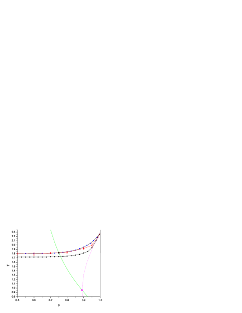
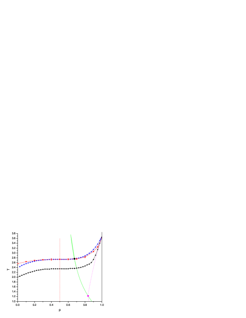


The measured equilibrium energy per bond is slightly higher than the random bond energy for and slightly lower for .
To within the high numerical precision the estimated at the NL-FK intersection point is independent of down to , Figures 3 and 4. The observed absence of finite scaling corrections at the NL also follows from Nishimori’s general statement quoted above nishimori:86 . For -values to the left and right of there are weak finite size effects of opposite signs. This absence of mean finite size scaling deviations arises because depends only on the energy. Other parameters can still show finite size scaling deviations hasenbusch:08 . The large size limits for and remain equal to each other to within the numerical precision of the points imaoka:97 over the strong disorder range of extending from to in the square lattice, and from to in the triangular lattice. Over these ranges of the satisfied bonds at are very close to being uncorrelated; for instance at on the square lattice which remains near to the uncorrelated value of . The further randomness introduced by the FK decimation is sufficient to render the active bond positions essentially uncorrelated. The imaoka:97 (or which has been measured here with higher precision) is rather insensitive to within this range, so that the measured is similar to the exact on both lattices. For both lattices in the more strongly ferromagnetic ranges , and in the range near to the fully frustrated limit in the triangular lattice, . At these concentrations the satisfied bonds are significantly correlated at and the FK decimation does not sufficiently compensate the correlations so as to produce randomness among the active bonds.
IV Damage spreading numerical results in dimension two
For dimension two the critical temperatures below which the long time large heat bath damage spreading tends to a non-zero value are also shown in Figures 1 and 2. The values given are obtained from extrapolating data at increasing sizes, Figures 5 and 6, to infinite size. On the basis of data for square and cubic lattices at it was conjectured earlier that dearcangelis:91 ; campbell:94 ; yamaguchi:10 as is the case in the pure ferromagnet limit. However the present data demonstrate that while the curves for and lie near together and are of very similar shape, in particular both being almost independent of for the range near , it is clear that except when tends to the ferromagnetic limit . So unfortunately it is not possible to define a unique joint ”dynamic transition temperature”. We will see that this is true also in higher dimensions.
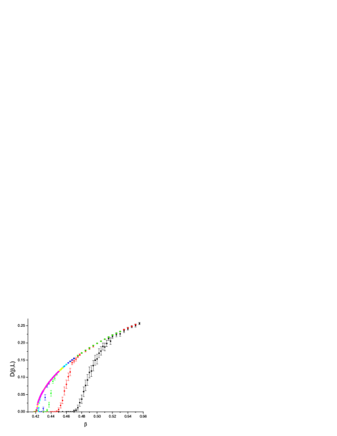
The present accurate critical value for the strong disorder square lattice is in good agreement with the earlier value campbell:91 and is very close to the ”regular to chaotic” dynamic transition temperature estimated for the same lattice in Ref. bernard:10 from the divergence of the coupling time with , where the data indicate a transition at .
V Dimensions three, four and five
It is numerically much more demanding to estimate precisely through direct measurements (as in imaoka:97 ), in particular allowing for finite size effects, than to estimate to the same level of accuracy. For cubic lattices in dimensions three, four and five the random bond critical concentrations though not exact have been estimated to very high precision, , and respectively lorenz:98 ; dammer:04 . Using the exact NL-FK intersection point expressions, Eqs. (6) and (7), one thus has and in dimension three, and in dimension four, and and in dimension five. Hence as and can be taken as known almost exactly, it is sufficient to estimate numerically (allowing carefully for finite size corrections) to obtain an accurate estimate of the ratio for each dimension.

The equilibrium damage was measured for given as a function of , and the results were extrapolated to obtain an estimate of the value at which falls to zero, Figures 5 and 6. There is a clear envelope curve for all in each case, with the data points leaving the curve later and later as increases. There are various ways to extrapolate to infinite . One efficient method is to fit the envelope points assuming that near the behavior follows and adjusting to obtain a straight line. We have also used a simple scaling formula to verify. Of course, a certain statistical uncertainty will enter depending on which to include in the fitting process which we take into account in the final error estimate.
The infinite damage spreading temperatures were estimated for the central values of in the three dimensions : in dimension three, in dimension four, and in dimension five. The observed ratios are equal to and respectively. In dimension three is indistinguishable from , while in dimensions four and five the values appear tantalizingly close but not identical. We have no explanation for the striking similarity between the two temperatures for the particular case of dimension three. Adding a little more detail for this particular case, the individual were estimated to an accuracy of for , for , for and for . Using the exponent gives a projected that depends only to a very small degree on which are included in the fit (though we always include ). We receive a median value of and a standard deviation of giving us . Similar methods were used to estimate for the other dimensions.
As in dimension two, the curve for is almost flat over a wide range of around for dimensions three and four, Figures 7 and 8 (the case of dimension five was not studied). These data are for fixed ( and respectively) so the values are not quite equivalent to the values quoted for at .
Judging from the behavior observed in dimension two, it seems very plausible to assume that the ratio is always practically independent of in the strong disorder regime .
It can be noted that numerical data for the time dependence of the autocorrelation function at all temperatures in two dimensional fully frustrated systems have been interpreted in terms of exponential relaxation with logarithmic corrections due to vortex-vortex interactions walter:11 . The results indicate that in these systems (which have well established FK and damage transitions) there is no dynamic critical temperature in the Ogielski sense ogielski:85 .
VI Damage clusters
It is of interest to examine in some detail the damage clusters in dimension two where they can be readily visualized. Keeping and letting (or at least allowing for equilibration) how does the damage actually spread? Note that we define a cluster as a connected component in the lattice induced by the damaged sites, i.e. a maximal set of damaged sites such that there is a lattice path (made up of horizontal and vertical steps) between each pair. The sum of the individual cluster sizes is thus the damage without normalization, i.e. . We have collected data on cluster sizes for . For we have only used the square lattice, not the triangular lattice.
What we see in a square lattice snapshot at near and at any arbitrary fixed time is not, as in the case for percolation (including FK percolation) or random graphs near , the formation of a giant cluster, but rather a large number of very small clusters. At subsequent times the clusters evolve and flutter through the lattice. An example is shown in Fig. 9


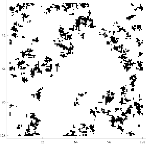
The measurements take place as above for the damage spreading; starting from random (infinite temperature) spin configurations, at each time step we update randomly selected sites, then search for all clusters and their sizes. On a measurement we collect the number of clusters, the average cluster size, the size of the largest cluster and the size of a randomly selected cluster. As before, we collect measurements from each sample after discarding between and time steps (depending on ) to allow for equilibration of the damage spreading. We then average over the time steps to get the average for a particular sample. The data are then averaged over the samples; we have only used eight samples in each case for the cluster measurements (for the damage speading we used between 8 and 128 samples depending on lattice size). In all cases we have set .
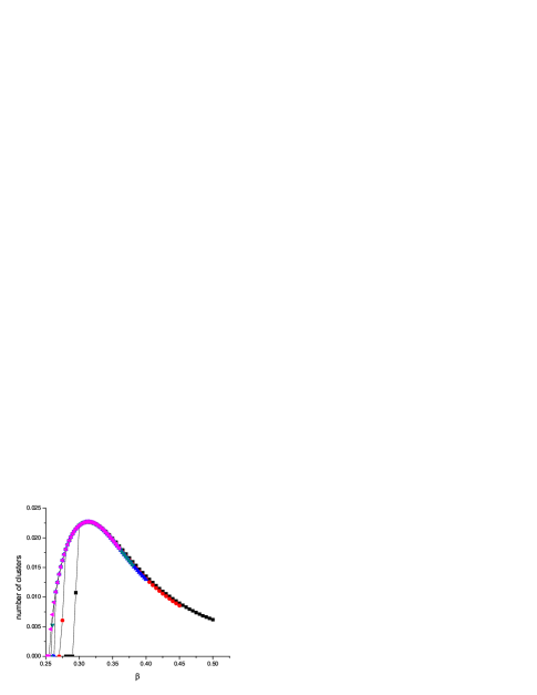
First we discuss the expected number of clusters, which we denote . In Figure 10 we plot versus for the simple cubic lattice. Equivalent behavior is found also for . Note that for the square lattice all lattice sizes agree on a global maximum probability located at , where . For we obtain and , for we get and , while gave and . Thus the damage is always distributed over clusters.
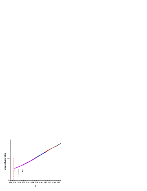
With so many clusters the average cluster at each time step must be rather small. We measure the number of damaged sites and the number of clusters , giving us the mean cluster size at each time step. The normalized time average (and then the sample average, though the sample variation is very small), is then . In Figure 11 we plot versus , again for . The curve clearly suggests a positive right limit at . To estimate this limit we fit a simple expression to the points resulting in . We estimated the right limits corresponding to to be respectively , , and sites at . One could alternatively define as the average damage divided by the average number of clusters. This is not strictly the same as our present definition (mean ratio versus ratio of the means) but the difference is of course vanishingly small here. For example, the maximum in Figure 10 at gives and the number of damaged sites, see Figure 6, is . Hence the average cluster size is roughly which matches Figure 11.
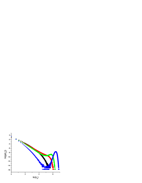
We end this section with a final remark concerning the distribution of cluster sizes. At each time step we here pick one cluster uniformly at random and measure its size. In Figure 12 we show a set of size distributions (or density functions) as vs for a range of for . They all have a high value at size (many isolated sites) and then drop quickly. They can be expected to behave like this since the mean size is between and in this temperature range. However, for (or thereabout) the distributions show a second, and rather wide, maximum located in the neighborhood of the total damage . This can be understood as follows. Suppose for the sake of argument that the damaged sites are distributed at random in space. (This is only approximate as correlations between damage sites should be allowed for). Then when exceeds the site percolation concentration there will exist a single ”giant” percolating cluster of damaged sites together with residual small clusters. As increases further the percolating cluster will contain almost all the damaged sites. On this criterion the peak should appear in the distribution at and in dimensions and respectively which gives an indication in rough agreement with the data. Indeed in the case of the square the peak never appears which is consistent with the fact that never approaches . For the dimensions where the peak does appear the global parameters, in particular , increase smoothly with and show no sign of any critical behavior as the giant cluster forms.
VII Conclusion
The exact values of the coordinates of the intersection point where the Fortuin-Kasteleyn transition line crosses the Nishimori line can be derived for an RBIM from the analytic condition that satisfied bonds are uncorrelated on the NL nishimori:86 . On any lattice this leads to the exact expressions and yamaguchi:10 ; campbell:94 where is the standard random bond percolation concentration for the particular lattice. For lattices in dimension two (and probably in higher dimensions also) the uncorrelated bond condition remains a very good approximation at the FK transition temperature over a wide strong-disorder region spanning .
In pure ferromagnets . The conjectured equivalence for the RBIM between the FK transition temperature and the heat bath damage spreading temperature , dearcangelis:91 ; campbell:94 ; yamaguchi:10 , separating an exponential from a chaotic dynamic regime has been tested at on simple cubic lattices in dimensions two, three, four and five. It holds to within in dimension three, to within in dimension four, and to in dimension five. The equivalence appears always to be a good approximation. We have no explanation to propose for the quasi-equality in the case of dimension three.
For the square and triangle lattices the difference is larger : and respectively.
The FK transition in the strong-disorder regime close to can thus be said to be well understood. However the basic physical condition determining the the damage spreading transition temperature, which plays an important role in limiting perfect equilibration in RBIMs, and its proximity to the FK transition, remains unclear.
VIII Acknowledgements
We are very grateful for enlightening remarks by H. Nishimori, C. Yamaguchi, R. Ziff and W. Krauth. The computations were performed on resources provided by the Swedish National Infrastructure for Computing (SNIC) at High Performance Computing Center North (HPC2N).
References
- (1) R.B. Griffiths, Phys. Rev. Lett. 23, 17 (1969).
- (2) Y. Matsuda, H. Nishimori and K. Hukushima, J. Phys. A: Math. Theor. 41, 324012 (2008).
- (3) H. Nishimori, Prog. Theor. Phys. 66, 1169 (1981).
- (4) C. M. Fortuin and P. W. Kasteleyn, Physica 57, 536 (1972).
- (5) A. Coniglio and W. Klein, J. Phys. A 13, 2775 (1980).
- (6) A. Coniglio, F. di Liberto, G. Monroy, and F. Peruggi, Phys. Rev. B 44, 12 605 (1991)
- (7) L. de Arcangelis, A. Coniglio, and F. Peruggi, Europhys. Lett. 14, 515 (1991).
- (8) V. Cataudella, Physica A 183, 249 (1991).
- (9) M. Zhang, C.Z. Yang, Europhys. Lett. 22 (1993) 505.
- (10) B. Derrida and G. Weisbuch, Europhys. Lett. 4, 657 (1987).
- (11) B. Derrida, Phys. Rep. 184, 207 (1989).
- (12) L. de Arcangelis, A. Coniglio, and H. Herrmann, Europhys. Lett. 9, 749 (1989).
- (13) I. A. Campbell and L. de Arcangelis, Physica 178, 29 (1991).
- (14) A. T. Ogielski, Phys. Rev. B 32, 7384 (1985).
- (15) R. H. Swendsen and J.-S. Wang, Phys. Rev. Lett. 58, 86 (1987).
- (16) U. Wolff, Phys. Rev. Lett. 62, 361 (1989).
- (17) J. Propp and D. Wilson, Random Struct. Algorithms , 9, 223 (1996).
- (18) E.P. Bernard, C. Chanal, and W. Krauth, Europhysics Lett. 92, 60004 (2010).
- (19) I.A. Campbell and L. Bernardi, Phys. Rev. B 50, 12643 (1994).
- (20) C. Yamaguchi, arXiv:1004.0654
- (21) H. Nishimori, Prog. Th. Phys. 76, 305 (1986).
- (22) H. Nishimori, ”Statistical Physics of Spin Glasses and Information Processing: An Introduction” (Oxford University Press, 2001), p.51.
- (23) S. Prakash, A. Coniglio, and H.E. Stanley, Phys. Rev. E 49, 2742
- (24) V. Cataudella, A. Coniglio, L. de Arcangelis, and F. di Liberto, Physica A 192, 167 (1993).
- (25) H. Imaoka, H. Ikeda, and Y. Kasai, Physica A 246 (1997) 18
- (26) C. Chanal and W. Krauth, Phys. Rev. Lett. 100, 060601 (2008).
- (27) C. Chanal and W. Krauth, Phys. Rev. E 81, 016705 (2010).
- (28) F.D. Nobre, Phys. Rev. E 64, 046108 (2001).
- (29) C. Wang et al., Ann. Phys. 303, 31 (2003).
- (30) C. Amoruso and A. K. Hartmann, Phys. Rev. B 70, 134425 (2004).
- (31) F. Parisen Toldin et al., J. Stat. Phys. 135, 1039 (2009).
- (32) C.K. Thomas and H.G. Katzgraber, Phys. Rev. E 84, 040101(R) (2011)
- (33) R. Häggkvist and P.H. Lundow, J. Stat. Phys. 108,429 (2002).
- (34) M. Hasenbusch, F.P. Toldin, A. Pelissetto, and E. Vicari, Phys. Rev. E 77, 051115 (2008).
- (35) C.D. Lorenz and R.M. Ziff, Phys. Rev. E 57, 230 (1998).
- (36) S.M. Dammer and H. Hinrichsen, J. Stat. Mech: Theory Exp. 7, 07011 (2004).
- (37) J.-C. Walter and C. Chatelain, arXiv:1112.4666.