The Design and Algorithms of
a Verification Condition Generator

FreeBoogie

Radu Grigore

The thesis is submitted to University College Dublin for the degree of PhD in the College of Engineering, Mathematical & Physical Sciences.

March 2010

School of Computer Science and Informatics

Head of School: Prof. Joe Carthy

Supervisor: Assoc. Prof. Joseph Roland Kiniry

Second supervisor: Prof. Simon Dobson

Summary

This dissertation belongs to the broad field of formal methods, which is, roughly, about using mathematics to improve the quality of software. Theoreticians help by teaching future programmers how to understand programs and how to construct them. Once people use mathematical techniques to do something, it is usually a matter of time until computers take over. Researchers in applied formal methods try to produce tools that that help programmers to write high-quality new code and also to find problems in old code. Spec^♯ is one attempt to produce such a tool. Looking at its backend, the Boogie tool, I noticed questions that begged to be answered.

At some point the program is brought into passive form, meaning that assignments are replaced by equivalent statements. It was clear that sometimes the passive form was bigger than necessary. Would it be possible to always compute the best passive form? To define precisely what ‘best’ means one first needs a precise definition of what constitutes a passive form. A part of the dissertation gives such a precise definition and explores what follows from it. Briefly, there are multiple natural meanings for ‘best’, for some of them it is easy to compute the ‘best’ passive form, for others it is hard.

Later the program is transformed into a logic formula that is valid if and only if the program is correct. There are two ways of doing this, based on the weakest precondition and based on strongest postcondition, but it was unclear what is the trade-off involved in choosing one method over the other.

One use-case for program verifiers is to monitor programmers writing new code and point out bugs as they are introduced. Batch processing is bound to be inefficient. Is there a way to reuse the results of a run when the program text changes as little as adding a statement or tweaking a loop condition? The answer is related to Craig interpolants.

Another question is why the Boogie tool checks only for partial correctness, and does not perform other analyzes as well. In particular, checking for semantic reachability of Boogie statements may reveal a wide range of problems such as inconsistent specifications, doomed code, bugs in the frontend of Spec^♯, and high-level dead code. Of course, one can manually insert assert false statements, but this is cumbersome. Also, the dissertation shows that it is possible to solve the task much more efficiently than by simply replacing each statement in turn with assert false.

Chapter 1 Introduction

“The purpose of your paper is not $\ldots$ to describe the WizWoz system. Your reader does not have a WizWoz. She is primarily interested in re-usable brain-stuff, not executable artifacts.”
— Simon Peyton-Jones [145]

1.1 Motivation

Ideal programs are correct, efficient, and easy to evolve. Tools can help with all three aspects: Type-checkers ensure that certain classes of errors do not occur, profilers identify performance hot-spots, and IDEs (integrated development environments) refactor programs. Automation allows humans to focus on the interesting issues. Knuth [109] put it differently: “Science is knowledge which we understand so well that we can teach it to a computer; and if we don’t fully understand something, it is an art to deal with.” For example, a bit string can represent both a text and an integer, we understand well how to check that a program does not mix the two interpretations, and we leave the task to type-checkers. If, on the other hand, we want to check that a program computes the transitive closure of a graph we usually do it by hand.

⬇ 1 requires square(G); 2 requires (forall i; G[i][i]); 3 ensures (forall i, j; G[i][j] == path(old(G), i, j)); 4{ final int n = G.length; 5 for (int k = 0; k < n; ++k) invariant (forall i, j; G[i][j] == pathK(old(G), i, j, k)); 6 for (int i = 0; i < n; ++i) 7 for (int j = 0; j < n; ++j) 8 G[i][j] = G[i][j] || (G[i][k] && G[k][j]); 9} 10 11axiom (forall G, i, j, k; pathK(G, i, j, k) = G[i][j] || (exists q; q<k && G[i][q] && pathK(G, q, j, k))); 12axiom (forall G, i, j; path(G, i, j) = pathK(G, i, j, G.length));

Figure 1.1: An example of what program verifiers can ideally do

A program verifier automatically checks whether code agrees with specifications. Figure 1.1 shows an example. Variables $i$, $j$, $k$, and $q$ range over nonnegative integers. The code is an implementation of the Roy–Warshall algorithm [158, 176]. The programmer spent energy to specify what the algorithm does (requires, ensures) and how it works (invariant). In words, $\mathit{path}(G,i,j)$ means that there is a path $i\leadsto j$ in the graph $G$, and $\mathit{pathK}(G,i,j,k)$ means that there is such a path whose intermediate nodes come only from the set $0\mathinner{\ldotp\ldotp}k-1$. The example illustrates what program verifiers ought to be able to do.

Note that it is trivial to establish the invariant (because pathK reduces to $G$ when $k=0$) and to infer the postcondition from the invariant (because pathK reduces to path when $k=n$). Proving that the invariant is preserved is trickier than it might seem mainly because of the in-place update, but could conceivably be done automatically. The proof of the invariant is sometimes omitted from informal explanations of the algorithm, but the information contained by the definitions of path and pathK is always communicated. The long term goal illustrated here is: A program verifier should be able to automatically check a program even when its annotations contain no more than what we would say to a reasonably good programmer to explain what the code does and how it works.

From an engineering perspective, program verifiers are similar to compilers. The input is a program written in a high-level language, and the output is a set of warnings (or errors) that indicate possible bugs. For a good program verifier, the lack of warnings should be a better indicator that the program is correct than any human-made argument. The architecture often consists of a front-end that translates a high-level language into a much simpler intermediate language, and a back-end that does the interesting work. The same back-end may be connected to different front-ends, each supporting some high-level language. The back-end is itself split into a VC (verification condition) generator and an SMT (satisfiability modulo theories) solver. A few alternatives to this architecture are discussed later (Section 1.3).

The VC generator is a trusted component of program verifiers. Therefore it is important to study it carefully, including its less interesting corners. This dissertation shows that even such corners come to life when analyzed in detail from the point of view of correctness and efficiency. The insights gained from such an analysis sometimes lead to simpler and cleaner implementations and sometimes lead to more efficient implementations.

1.2 History

In 1957, ‘programming’ was not a profession. At least that’s what Dijkstra was told [64]. “And, believe it or not, but under the heading profession my marriage act shows the ridiculous entry theoretical physicist!” That is only one story showing that in those times programmers were second class citizens and did not have many rights. Their predicament was, however, well-deserved: They did not care about the correctness of programs, and they did not even grasp what it means for a program to be correct! A few bright people changed the situation. In 1961 McCarthy [130] published the first article concerned with the study of what programs mean. The article is focused on handling recursive functions without side effects, which corresponds to the style of programming used nowadays in pure functional languages like Haskell [146]. Six years later, in 1967, Floyd [75] showed how programs with side effects and arbitrary control flow can be handled formally. He acknowledges that some ideas were inspired by Alan Perlis. He emphasized the view of programs as flowgraphs (or, more precisely, flowcharts). His method is usually known under the name “inductive assertions.” The method was popularized by Knuth [108]. In 1969, Hoare [91] introduced an axiomatic method of assigning meanings to programs that appealed more to logicians than to algorithmists. Although the presentation style is very different, Hoare states that “the formal treatment of program execution presented in this paper is clearly derived from Floyd.” Based on Hoare’s work, Dijkstra [65] introduced in 1975 yet another way of defining the meaning of programs based on predicate transformers such as the weakest precondition transformer. He did so in the context of a language (without goto) called “guarded commands,” which provided the main inspiration for the Boogie language.

It is revealing that all the authors mentioned in the previous paragraph received the Turing Award, although not necessarily for closely related topics:

• Alan Perlis: “For his influence in the area of advanced programming techniques and compiler construction.”

• John McCarthy: “For his major contributions to the field of artificial intelligence.”

• Edsger W. Dijkstra: “[For] his approach to programming as a high, intellectual challenge; his eloquent insistence and practical demonstration that programs should be composed correctly, not just debugged into correctness; and his illuminating perception of problems at the foundations of program design.”

• Donald E. Knuth: “For his major contributions to the analysis of algorithms and the design of programming languages.”

• Robert W. Floyd: “For having a clear influence on methodologies for the creation of efficient and reliable software, and for helping to found the following important subfields of computer science: the theory of parsing, the semantics of programming languages, automatic program verification, automatic program synthesis, and analysis of algorithms.”

• C. A. R. Hoare: “For his fundamental contributions to the definition and design of programming languages.”

Most researchers now prefer to define programming languages from an operational point of view. Such definitions (1) tend to be more intuitive for programmers and (2) correspond directly to how interpreters are implemented. Plotkin’s lecture notes [147] constitute the first coherent and comprehensive account of this approach. Much later, in 2004, Plotkin put together a historical account [148] of how his ideas on structural operational semantics crystallized. He points to alternative ways of handling the goto statement. He cites McCarthy [130] as inspiring him to simplify existing work, and credits Smullyan [162] for the $\frac{\text{up}}{\text{down}}$ rules. He also relates operational semantics to denotational semantics [20].

All these developments are based on even older work. In the nineteenth century Hilbert advocated a rigorous approach to mathematics: It should be possible in principle to decompose any mathematical proof into a finite sequence of formulas $p_{1}$, $p_{2}$, $\ldots$, $p_{n}$ such that each formula is either an axiom or is obtained from previous formulas by the application of a simple transformation rule. (Such a sequence is a proof of all the formulas it contains.) The set of axioms is fixed in advance and is called theory. The set of transformation rules is also fixed in advance and is called calculus. Without looking at the language used to express formulas, there is not much more that can be said about this process. If the language is propositional logic ($\top$, $\bot$, and variables, connected by $\lnot$, $\lor$, and $\land$), then we can evaluate a formula to $\top$ or $\bot$ once a valuation—assignment of values to variables—is fixed. A model is a valuation that makes all axioms evaluate to $\top$. A formula is valid when it evaluates to $\top$ for all models. A calculus is sound if it produces only valid formulas starting from valid axioms; a calculus is complete if it can produce all the valid formulas. Even if a sound calculus is used, anything can be derived if we start with an inconsistent theory, one that has no model. These observations generalize for other languages like fol, hol (higher order logic), and lambda calculus. The notion of evaluating formulas is ‘operational,’ while the calculus feels more like the axiomatic approach to programming languages. The intimate connection between proofs and programs is explored in a tutorial style by Wadler [174].

1.3 Related Work

The previous section gave (intentionally) a very narrow view of modern research on program verification. It is now time to right that wrong, partly. Because the field is so vast, we still do not look at all important subfields. For example, no testing tool inspired by theory is mentioned.

The sharpest divide is perhaps between tools mainly informed by practice and tools mainly informed by theory. The authors of FindBugs [96], PMD [15], and FxCop [8] started by looking at patterns that appear in bad code and then built specific checkers for each of those patterns. Hence, those tools are collections of checkers plus some common functionality that makes it easy to implement and drive such checkers. Crystal [6], Soot [167], and NQuery [13] are stand-alone platforms that make it easy to implement specific checkers. Rutar et al. [160] compare a few static analysis tools for Java, including FindBugs and PMD, from a practical point of view.

Tools informed by theory lag behind in impact, but promise to offer better correctness guarantees in the future. These tools can be roughly classified by the main techniques used by their reasoning core.

Model checking [48] led to successful hardware verifiers like RuleBase [17, 35]. A model checker verifies whether certain (liveness and safety) properties hold for a certain state graph—the ‘model.’ The properties are written in a temporal logic, such as LTL or CTL; the model is a Kripke structure and is represented usually in some implicit form that tries to avoid state explosion. SPIN [18, 93] and NuSMV [14, 47] are generic model checkers and each has its input language. Hardware model checkers start by transforming a VHDL or Verilog description into a state graph, while software model checkers start by transforming a program written in a language like Java into a state graph. Software model checkers that are clearly under active development include the open source Java Pathfinder [12, 171] and CHESS [4, 137] (for Win32 object code and for CIL). SLAM [22], a commercially successful tool developed by MSR, uses a combination of techniques, including model checking, to verify several properties of Windows drivers. Another noteworthy software model checker is BLAST [2, 38] (for C). Bogor [3, 155] is a framework for developing software model checkers.

The input of theorem provers [156, 157] is a logic formula. Usually, when the language is fol, the theorem prover tries to decide automatically if the input is valid; usually, when the language is hol the theorem prover waits patiently to be guided through the proof. The former are proof finders, while the later are proof checkers. The distinction is not clear cut: Sometimes, the steps that an interactive prover “checks” are as complicated as some of the theorems that are “proved” automatically. Still, in practice the distinction is important: Automatic theorem provers tend to be fast, while interactive theorem provers tend to be expressive.

The most widely used hol provers are Coq [5, 37], Isabelle/HOL [9, 10, 140], and PVS [16, 143]. The gist of such provers is that they (should) rely on a very small trusted core. One way to use such theorem provers for program verification is to do everything in their input language. For example, Leroy [124] implemented a compiler for a subset of C in Coq’s language, formulated theorems that capture desired properties of a C compiler, and proved them. Since Coq comes with a converter from Coq scripts to OCaml [152] programs, the compiler is executable. (The converter fails if non-constructive laws such as the excluded middle are used.) Another approach is to introduce notation that makes the Coq/HOL/Isabelle script look ‘very much’ like the program that is being run [128]. Yet another approach is to use hol as the target language of a VC generator (see [40, 31, 168]).

The first approach, that of interactively programming and proving in the same language, is also used with ACL2 [1, 105], whose input language is not higher-order.

Provers that handle only fol do not usually require programmers to interact directly with them. SMT solvers [30], like Z3 [59] and CVC3 [29], are designed for program verification. The modules of an SMT solver—a SAT solver and decision procedures for various theories—communicate through equalities. This architecture dates back to Nelson and Oppen [139]. The theories are axiomatizations of things that occur frequently in programs, like arrays, bit vectors, and integers. A specialized decision procedure can handle integers a lot more efficiently than a generic procedure. The extra speed comes at the cost of increasing considerably the size of the trusted code base. To have the best of both worlds, speed and reliability, SMT solvers may produce proofs that can be later checked by a small program [136]. However, this poses the extra challenge of producing proof pieces from each decision procedure and then gluing them together. Simplify [61] was for many years the solver of choice for program verification. It has a similar architecture (being co-developed by Nelson), but understands a language slightly different than the standardized SMT language [28].

Throughout this dissertation, the term ‘program verifier’ is used usually in a very restricted sense. It refers to a tool that

1. uses an SMT solver as its reasoning core,

2. has a pipeline architecture and an intermediate language, and

3. can be used to generate warnings just like a compiler.

The pipeline architecture with an intermediate language is typical in translators and compilers [142].

Many tools fit this narrow definition, including ESC/Java [71], the static verifier in Spec^♯ [26] (for C^♯), HAVOC [114] (for C), VCC [50] (for C), Krakatoa [70] (for Java), the Jessie plugin in Frama-C [7] (for C), and JACK [31] (for Java). ESC/Java and JACK support JML [115] (the Java modeling language), an annotation language for Java that has wide support, a reference manual, and even (preliminary and partial) formal semantics [116]. Frama-C supports ACSL [32], another of the few annotation languages with an adequate reference manual.

The intermediate language, or at least the intermediate representation, used by these tools is much better specified. ESC/Java uses a variant of Dijkstra’s guarded commands [65] that has exceptions. Spec^♯, HAVOC, and VCC, which are developed by Microsoft Research, use the Boogie language [118, 122]. Krakatoa and Frama-C, which are developed by INRIA, use the Why language [70]. The Boogie language (and the associated verifier from Microsoft Research) was used also as a high-level interface to SMT solvers in order to verify algorithms and to explore encoding strategies for high-level languages [23, 164].

Many tools have more than one reasoning engine. JACK uses Simplify and Coq. The Why tool uses a wide range of theorem provers: Coq, PVS, Isabelle/HOL, HOL 4, HOL Light, Mizar; Ergo, Simplify, CVC Lite, haRVey, Zenon, Yices, CVC3. SLAM uses both a model checker and the SMT solver Z3.

The Boogie tool, FreeBoogie, and the Why tool are fairly big pieces of code that convert a program written in an intermediate language into a formula that should be valid if and only if the program is correct. Moore [135] argues that a better solution is to explicitly write the operational semantics, which leads to a much smaller VC generator. It is not clear what impact this has on speed. However, the technique is most intriguing and it would be interesting to pursue it in the context of Boogie and Why. (Moore uses ACL2.) Other tools, like KeY [33] (for Java, using dynamic logic [87]), jStar [66] (for Java, using separation logic [153]), and VeriFast [98] (for C, using separation logic [153]), avoid the VC generation step because they rely on symbolic execution [106]. This means, very roughly, that instead of turning the program into a proof obligation into one giant step, they ‘execute’ the program and they keep track of the current possible states using formulas. At each execution step they may use the help of a reasoning engine. (Note that at this level of abstraction and hand-waving there is not much difference between symbolic execution and abstract interpretation [55].)

With so many tools, it is surprising that they do not have a more serious impact in practice. On this subject one can only speculate. It is probably true that a closer collaboration between theoreticians and practitioners would ameliorate the situation. But it is also true that researchers still have much work to do on known problems. The expressivity of specification languages is a family of such problems. For example, it is still considered a research challenge to annotate particularly simple patterns, like the Iterator pattern [85] or the Composite pattern [164]. Speed is another problem. As any (non-Eclipse) computer user will tell you, the number of users of a program tends to decrease with its average response time. Since program verifiers are intended to be used similarly with compilers, their speed is naturally compared with that of compilers. Right now, the response times of program verifiers are higher and have a greater variance.

It is, of course, bothersome that in today’s state of affairs it is hard to annotate the Iterator pattern properly in many verification methodologies. (Otherwise it would not have been the official challenge of SAVCBS 2006.) But we should not expect practitioners to annotate such things at all, just as we should not expect them to state the invariant $0\leq i\leq n$ on the omnipresent for loop. In general, usable verification tools should embody knowledge that is common to people in a specific domain. There is some work on tackling typical exercises in an introductory programming course [121] and there is also work in encoding traditional mathematical knowledge in verifiers [42].

A choice that may have seemed unusual is the use of the name ‘Roy–Warshall,’ instead of the more standard ‘Floyd–Warshall,’ for the algorithm in Figure 1.1. There are many algorithms with the shape

(1.1) for $$k i j a_{ij}\leftarrow a_{ij}\circ(a_{ik}\bullet a_{kj})$$ do for , do

and they are sometimes known under the name “the $kij$ algorithm.” Roy [158] and Warshall [176] noticed independently that $\circ=\lor$ and $\bullet=\land$ solves the transitive closure problem. Floyd [74] noticed that $\circ=\min$ and $\bullet=+$ solves the all pairs shortest paths problem. (He did this five years before assigning meanings to programs.) Although less clear, other earlier algorithms are instantiations of the $kij$ schema. Kleene [107] proved that every finite automaton corresponds to a regular expression. His proof is constructive and is now known as Kleene’s algorithm. The Gauss–Jordan method for solving systems of linear equations is another example. Pratt [150] discusses the $kij$ algorithm in general terms.

1.4 A Guided Tour

The content of this dissertation touches on issues related to software engineering, compilers, programming languages, algorithm analysis, and theorem provers. It is often abstract and theoretical, but sometimes descends into implementation details. Therefore, there are plenty of opportunities for a reader to find something enjoyable. Of course, there are even more opportunities for a reader to find something not enjoyable, especially if the reader has a strong preference for one sub-field of computer science. Fortunately, the dissertation does not stem from one big contribution, but rather from many smaller ones that are related and yet can be understood independently. The dependencies between chapters appear in Figure 1.2. Chapter 2 is very important, as it is required reading for all subsequent chapters.

Figure 1.2: Dependencies between chapters

The scope of the dissertation reflects the broad interests of the author. Often, broad texts say nothing about a lot, and are quite boring. The focus on a very specific part of a very specific type of static analysis tools and the focus on a very small subset of the Boogie language are meant to ensure enough depth.

My hope is that the dissertation will bring together at least two people from different sub-fields of computer science to work together on a common problem related to program verifiers.

Chapter 2 presents the syntax and the operational semantics of a subset of the Boogie language, which is used throughout subsequent chapters.

Chapter 3 presents what FreeBoogie does. Its architecture is sketched, including the interfaces between major components. The advantages and disadvantages of each important design decision are discussed, so that others who endeavor in similar tasks avail of our experience and avoid repeating our mistakes.

Chapter 4 presents how FreeBoogie replaces assignments by equivalent assumptions. The algorithm’s complexity is analyzed in detail and its goals are clearly defined. A natural variant of the problem is proved to be NP-hard.

Chapter 5 presents how FreeBoogie generates a prover query from a Boogie program, using either a weakest precondition transformer or a strongest postcondition transformer. In the process, we see how four types of assigning meanings to Boogie programs relate to each other: operational semantics, Hoare triples, weakest preconditions, and strongest postconditions. (Chapters 4 and 5 are based on [83].)

Chapter 6 presents how FreeBoogie exploits the incremental nature of writing code and annotations in order to improve its response times. The generic idea, of exploiting what is known from previous runs of the verifier, is refined and then proved correct. (This chapter is based on [84].)

Chapter 7 presents what FreeBoogie does to protect developers from making silly mistakes that render verification useless: Inconsistencies make everything provable. An algorithm that efficiently searches for inconsistencies is given and is analyzed. Experimental results show that it is practical. (This chapter is based on [101].)

Chapter 8 concludes the dissertation. Appendix A summarizes the notation used throughout the dissertation. The reader is advised to browse that appendix before continuing with the next chapter.

Software engineers and practitioners are likely to enjoy most Chapter 3. People with a formal background, like logicians and type theorists, are likely to enjoy most Chapters 5 and 6. Algorithmists are likely to enjoy most Chapter 4, 6 and 7. Developers of program verification tools are likely to enjoy most Chapters 6 and 7.

Chapter 2 The Core Boogie

“The boogie bass is defined as a left-hand rhythmic pattern, developed from boogie-woogie piano styles, that is played on the bass string.”
— Frederick M. Noad [141]

From now on almost all programs are written in the Boogie language, and almost all are written in a subset—the core Boogie—defined in this section. What is ‘core’ is relative to the topics discussed in this dissertation.

Figure 2.1 shows an implementation of sequential search. After the counter $i$ is initialized in line 2 the control goes nondeterministically to both labels $b$ and $d$. An execution gets stuck if it hits an assumption that does not hold. Since the conditions on the lines 3 and 5 are complementary, exactly one of the two executions will continue. (In general, the if statement of full Boogie may be desugared into a goto statement that targets two assume statements with complementary conditions.) The return statement is reached only if $i\geq\mathit{vl}$ or $v[i]=u$.

⬇ 1procedure indexOf(u : int, v : [int] int, vl : int) returns (i : int) { 2 a: i := 0; goto b, d; 3 b: assume i < vl && v[i] != u; 4 c: i := i + 1; goto b, d; 5 d: assume !(i < vl && v[i] != u); return; 6}

Figure 2.1: Boogie program with one loop and its flowgraph

The high-level constructs of full Boogie (such as if statements, while statements, and call statements) can always be desugared into the core that is formalized here. The concrete grammar of core statements appears in Figure 2.2. The statement assert $p$ means “when you reach this point, check that $p$ holds.” The statement assume $p$ means “continue to look only at executions that satisfy $p$.”

statement$\>\to$	label? (assignment $\mid$ assumption $\mid$ assertion $\mid$ jump) ;
label$\>\to$	id :
assignment$\>\to$	id := expression
assumption$\>\to$	assume expression
assertion$\>\to$	assert expression
jump$\>\to$	(goto id-tuple ) $\mid$ return
id-tuple$\>\to$	id (, id)∗

Figure 2.2: Syntax of core Boogie statements

The type system of full Boogie is rich, featuring polymorphic maps, bit vectors, and user-defined types, among others. Its expression language is similarly rich. Unlike in the case of statements, the VC generator implementation (henceforth known as FreeBoogie) does not desugar types and expressions into simpler ones. How they are treated, however, is not novel. For the sake of the presentation, only a few types and expressions are retained in the core, the ones in Figure 2.3.

type$\>\to$	primitive-type $\mid$ map-type
primitive-type$\>\to$	int $\mid$ bool
map-type$\>\to$	[ primitive-type ] type
expression$\>\to$	( quantifier id : type :: expression )
expression$\>\to$	unary-operator expression $\mid$ expression binary-operator expression
expression$\>\to$	expression [ expression ]
expression$\>\to$	id $\mid$ literal $\mid$ ( expression )
quantifier$\>\to$	forall $\mid$ exists
unary-operator$\>\to$	! $\mid$ -
binary-operator$\>\to$	+ $\mid$ - $\mid$ $<$ $\mid$ == $\mid$ && $\mid$ $||$
literal$\>\to$	true $\mid$ false $\mid$ 0 $\mid$ 1 $\mid$ 2 $\mid$ …

Figure 2.3: Syntax of core Boogie types and expressions

The syntax for the overall structure of core Boogie programs appears in Figure 2.4. Statements are preceded by variable declarations, in which the variables representing the input and the output are singled out. The keyword procedure is retained from full Boogie, where a program may contain more than one procedure and where there is also a call statement. Procedures are not included in the core, because there is nothing novel related to procedure calls in this dissertation. The mandatory return statement at the end of each body reduces the number of special cases that need to be discussed later. FreeBoogie inserts such a statement automatically during parsing, so the user does not have to end all procedures with return.

program$\>\to$	procedure id ( arguments? ) returns ( results? ) body
arguments, results$\>\to$	id : type (, id : type)∗
body$\>\to$	variable-declaration∗ statement∗ return ;
variable-declaration$\>\to$	var id : type ;

Figure 2.4: Structure of a (core) Boogie program

Typechecking core Boogie is straightforward: Figure 2.5 shows a representative sample of the typing rules. The judgment $\vdash p$ means that the program fragment $p$ is well-typed and the judgment $\vdash p:t$ means that the program fragment $p$ is well-typed and has the type $t$. The customary environment is omitted because it is fixed—it consists of all the variable typings appearing at the beginning of the program. The rules that are missing are similar to the ones given: For example, there is a rule that says that the expression appearing in an assumption must have the type bool (analogous to rule [asrt]).

$$\begin{array}[]{ccc}\frac{\exists t,\;\vdash v:t\;\land\;\vdash e:t}{\vdash v\boldsymbol{:=}e}\;\text{[asgn]}&&\frac{\vdash e:\mathbf{bool}}{\vdash\mathbf{assert}\;e}\;\text{[asrt]}\\ \\ \frac{\vdash e:\mathbf{bool}\quad\vdash f:\mathbf{bool}}{\vdash e\>\boldsymbol{\&\&}\>f:\mathbf{bool}}\;\text{[bool]}&&\frac{\vdash e:\mathbf{int}\quad\vdash f:\mathbf{int}}{\vdash e\>\boldsymbol{+}\>f:\mathbf{int}}\;\text{[arith]}\\ \\ \frac{\vdash e:\mathbf{int}\quad\vdash f:\mathbf{int}}{\vdash e\>\boldsymbol{<}\>f:\mathbf{bool}}\;\text{[comp]}&&\frac{\exists t,\;\vdash e:t\;\land\;\vdash f:t}{\vdash e\>\boldsymbol{==}\>f:\mathbf{bool}}\;\text{[eq]}\\ \\ \frac{}{\vdash\mathbf{true}:\mathbf{bool}}\;\text{[lit-bool]}&&\frac{}{\vdash\boldsymbol{0}:\mathbf{int}}\;\text{[lit-int]}\end{array}$$

Figure 2.5: Typing rules for core Boogie

Operational Semantics

The set of all variables is denoted by Variable. It can be thought of as the set of all identifiers or as the set of all strings. The set of all values is denoted by Value and it contains the set of booleans $\mathbb{B}=\{\top,\bot\}$. Stores assign values to variables.

(2.1) $$\mathit{Store} =\mathit{Variable}\to\mathit{Value}$$

(2.2) $$\sigma \in\mathit{Store}$$

Expressions assign values to a stores. Boolean expressions, called predicates, define sets of stores.

(2.3) $$\mathit{Expression} =\mathit{Store}\to\mathit{Value}$$

(2.4) $$\mathit{Predicate} =\mathit{Store}\to\mathbb{B}$$

(2.5) $$p,q,r \in\mathit{Predicate}$$

According to the syntax, the program is a list of statements, which means that we can assign counters $0$, $1$, $2$, $\ldots$ to them. To simplify the presentation, we will assume that all labels are counters (in the proper range). The state of a Boogie program is either the special error state or a pair $\langle\sigma,c\rangle$ of a store $\sigma$ and a counter $c$ of the statement about to be executed. The following rules define a relation $\leadsto$ on states, thus giving an operational semantics for the core of the Boogie language.

(2.6) $$\frac{p\;\sigma}{\langle\sigma,c:(\mathbf{assume}/\mathbf{assert}\;p)\rangle\leadsto\langle\sigma,c+1\rangle}$$

(2.7) $$\frac{\lnot(p\;\sigma)}{\langle\sigma,c:(\mathbf{assert}\;p)\rangle\leadsto\mathit{error}}$$

(2.8) $$\frac{}{\langle\sigma,c:(v\mathtt{:=}e)\rangle\leadsto\langle(v\leftarrow e)\;\sigma,c+1\rangle}$$

(2.9) $$\frac{c^{\prime}\in\ell}{\langle\sigma,c:(\mathbf{goto}\;\ell)\rangle\leadsto\langle\sigma,c^{\prime}\rangle}$$

A rule $\frac{h}{\langle\sigma,\,c:\mathscr{P}\rangle\leadsto s}$ means that the program may evolve from state $\langle\sigma,c\rangle$ to the state $s$ if the hypothesis $h$ holds and if the counter $c$ corresponds to a statement that matches the pattern $\mathscr{P}$. For example, rule (2.9) says that $\langle\sigma,c\rangle$ may evolve into $\langle\sigma,c^{\prime}\rangle$ if the statement at counter $c$ matches the pattern goto $\ell$ and $c^{\prime}\in\ell$. The notation $p\;\sigma$ stands for the application of function $p$ to the argument $\sigma$. Space (that is, the function application operator) is left associative, has the highest precedence, and, as is customary, it is omitted if there is only one parenthesized argument that is not followed by another function application. The notation $(v\leftarrow e)$ used in rule (2.8) stands for a store transformer, defined as follows.

(2.10) $$(v\leftarrow e) :\mathit{Store}\to\mathit{Store}$$

(2.11) $$(v\leftarrow e)\;\sigma\;w =\begin{cases}\sigma\;w&\text{if $v\neq w$}\\ e\;\sigma&\text{if $v=w$}\end{cases}$$

Definition 1.

An execution of a core Boogie program is a sequence $s_{0}$, $s_{1}$, …, $s_{n}$ of states such that $s_{k-1}\leadsto s_{k}$ for all $k\in 1.\,.\>n$ and $s_{0}=\langle\sigma_{0},0\rangle$ for some arbitrary initial store $\sigma_{0}$.

Remark 1.

All executions are finite. This is an unusual simplification, but one that can be made as long as we do not investigate whether programs terminate.

The sources of nondeterminism in core Boogie are (1) the initial store $\sigma_{0}$ and (2) the goto rule (2.9) which allows multiple successors.

We say that an execution $s_{0}$, $s_{1}$, …, $s_{n}$ goes wrong if $s_{n}=\mathit{error}$. This can happen only if the last statement that was executed was an assertion. We say that that assertion was violated.

Definition 2.

A core Boogie program is correct when none of its executions goes wrong.

Boogie does not facilitate reasoning about termination. Throughout the dissertation the term “correct” will usually mean what is traditionally referred to as “partially correct.” Because we are not interested in termination, we do not distinguish between executions that reach an assumption that is not satisfied and executions that reach a return statement: both get stuck.

Let us look at an example. If we turn the labels of the program in Figure 2.1 (on page 2.1) into counters we obtain

⬇

0:    i := 0;

1:    goto 2, 5;

2:    assume i < vl && v[i] != u;

3:    i := i + 1;

4:    goto 2, 5;

5:    assume !(i < vl && v[i] != u);

6:    return;

for which one possible execution is

(2.12) $$\langle\sigma,0\rangle$$

(2.13) $$\langle(i\leftarrow 0)\;\sigma,1\rangle$$

(2.14) $$\langle(i\leftarrow 0)\;\sigma,2\rangle$$

(2.15) $$\big{(}i<\mathit{vl}\land v[i]\neq u\big{)}\;\big{(}(i\leftarrow 0)\;\sigma\big{)} (*)$$

(2.16) $$\langle(i\leftarrow 0)\;\sigma,3\rangle$$

(2.17) $$\langle(i\leftarrow i+1)\;((i\leftarrow 0)\;\sigma),4\rangle$$

(2.18) $$\langle(i\leftarrow i+1)\;((i\leftarrow 0)\;\sigma),5\rangle$$

(2.19) $$\lnot\big{(}i<\mathit{vl}\land v[i]\neq u\big{)}\;\big{(}(i\leftarrow i+1)\;((i\leftarrow 0)\;\sigma)\big{)} (*)$$

(2.20) $$\langle(i\leftarrow i+1)\;((i\leftarrow 0)\;\sigma),6\rangle$$

(The store $\sigma$ is arbitrary but fixed.) The lines marked with $(*)$ are not states but rather conditions that are assumed to hold. In order to evaluate those conditions we need to look inside the predicates. Every $n$ary function $f:(\mathit{Value}\to)^{n}\mathit{Value}$ has a corresponding function $f^{\prime}$ on expressions:

(2.21) $$f^{\prime} :(\mathit{Expression}\to)^{n}\mathit{Expression}$$

$$f^{\prime}\;e_{1}\ldots e_{n}\;\sigma =f\;(e_{1}\;\sigma)\ldots(e_{n}\;\sigma)$$

In particular, boolean functions have corresponding predicate combinators. By notation abuse, we write $\land$, $\lor$, $\ldots$ between booleans as well as between predicates. Also, the boolean constants $\top$ and $\bot$ are boolean functions with arity $0$, so we shall abuse them too and write $\top$ and $\bot$ for constant predicates. Similarly, we will lift the other operators. An example evaluation of a predicate follows.

$$\big{(}i<\mathit{vl}\land v[i]\neq u\big{)}\;\big{(}(i\leftarrow 0)\;\sigma\big{)}$$

$$=\quad (i<\mathit{vl})\;\big{(}(i\leftarrow 0)\;\sigma\big{)}\land(v[i]\neq u)\;\big{(}(i\leftarrow 0)\;\sigma\big{)}$$

$$=\quad i\;\big{(}(i\leftarrow 0)\;\sigma\big{)}<\mathit{vl}\;\big{(}(i\leftarrow 0)\;\sigma\big{)}\land\ldots$$

A predicate that consists of a variable $v$ is evaluated by reading the variable’s value from the store; a predicate that consists of a constant $c$ evaluates to that (lifted) constant. (For example, the predicate $0$ is lifted to the integer $0$.)

(2.22) $$v\;\sigma =\sigma\;v$$

(2.23) $$c\;\sigma =c$$

The evaluation continues as follows.

(2.24) $$i\;\big{(}(i\leftarrow 0)\;\sigma\big{)}<\mathit{vl}\;\big{(}(i\leftarrow 0)\;\sigma\big{)}$$

(2.25) $$=\quad (i\leftarrow 0)\;\sigma\;i<(i\leftarrow 0)\;\sigma\;\mathit{vl}$$

(2.26) $$=\quad 0<\sigma\;\mathit{vl}$$

And we conclude that for the previous example execution the initial store $\sigma$ must satisfy $0<(\sigma\;\mathit{vl})$.

A special case of (2.21) is equality. Equality between values is a function $=\;:\mathit{Value}\to\mathit{Value}\to\mathbb{B}$ that has a corresponding expression combinator $=\;:\mathit{Expression}\to\mathit{Expression}\to\mathit{Predicate}$. For example, we write $v=e$ for a predicate that defines the set of stores in which the variable $v$ and the expression $e$ evaluate to the same value.

We say that predicate $p$ is valid and we write $|p|$ when it holds for all stores.

(2.27) $$|p|=(\forall\sigma,\;p\;\sigma)$$

We will often need to say that two predicates delimit exactly the same set of stores, so we introduce a shorthand notation for it, which will also be useful when defining (syntactically) new predicates.

(2.28) $$(p\equiv q)=|p=q|$$

Finally, we shall abuse notation and write $(v\leftarrow e)\;p$ for predicates $p$, based on the fact that every store transformer $f:\mathit{Store}\to\mathit{Store}$ has a corresponding expression transformer $f^{\prime}$:

(2.29) $$f^{\prime} :\mathit{Expression}\to\mathit{Expression}$$

(2.30) $$f^{\prime}\;e\;\sigma =e\;(f\;\sigma)$$

This concludes the presentation of the core of Boogie that is used often in the next chapters.

Prior Work

The semantics given here for core Boogie correspond to the trace semantics of Leino [118]. Simple statements are treated essentially as input–output relations [90, Chapter 6]. Unusually, this chapter does not define explicitly any way to compose statements. Instead, a program counter and goto statements allow any control flowgraph, in the style of Floyd [75].

The full Boogie language [122] is more high-level and more user-friendly.

Chapter 3 Design Overview

“One of the best indications that a program is the result of the activity of design is the existence of a document describing that design.”
— Jim Waldo [175]

This chapter is rather dense. A cursory read will show how the later, more theoretical chapters fit together in the context of a real program; a careful read will serve as a guide to FreeBoogie’s source code for new developers.

3.1 An Example Run

⬇ 1procedure indexOf(x : T, a : [int] T, al : int) returns (i : int) { 2 i := 0; 3 while (i < al && a[i] != x) { i := i + 1; } 4}

Figure 3.1: A high-level Boogie version of Figure 2.1

The best way to understand how FreeBoogie works is to run it on a few examples and ask it to dump its data structures at intermediate stages. Figure 3.1 shows a Boogie program suitable for a first run. Notice that the language is not restricted to the core defined in Chapter 2. To peek at FreeBoogie’s internals use the command

fb --dump-intermediate-stages=log example.bpl

assuming that you wrote the content of Figure 2.1 in the file example.bpl and that FreeBoogie is correctly installed on your system. This will create a directory named log. The output of each processing phase of FreeBoogie appears in a subdirectory of log.

Such transformation phases include desugaring the while statement, desugaring the if statement, cutting cycles, eliminating assignments (Chapter 4), computing the VC (Chapter 5). Let us look briefly at the state of FreeBoogie after while and if statements are desugared. To do so we could look at the pretty-printed Boogie code but we can also look at the flowgraph that is dumped by FreeBoogie in the GraphViz [67] format. A command like

dot log/freeboogie.IfDesugarer/*.dot -Tpng > fig3.2.png

produces Figure 3.2. Such drawings of the internal data structures are very helpful in understanding FreeBoogie and in debugging it. For example, in Figure 3.2 we see that FreeBoogie introduces labels prefixed by $$ and a string like if or while, which hints to the origin of the label.

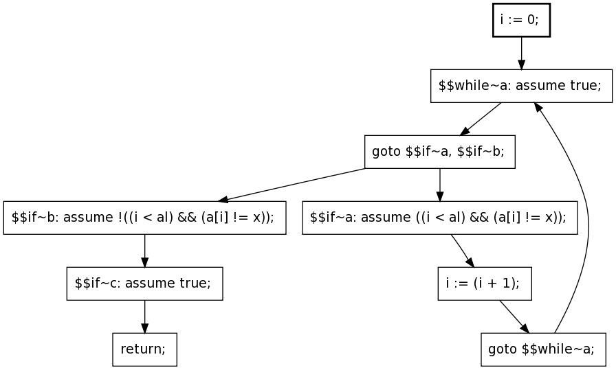
Figure 3.2: Flowgraph of a desugared version of Figure 2.1

The flowgraph is an example of auxiliary information that FreeBoogie computes after each transformation. The other pieces of auxiliary information are the symbol table and the types. The symbol table is a one-to-many bidirectional map between identifier definitions and identifier uses. The types are associated with expressions (and subexpressions).

To see the query that is sent to the theorem prover you must run a different command, this time shown in abbreviated form:

fb -lf=example.log -ll=info -lc=prover example.bpl

The log file example.log will contain everything sent to the prover. FreeBoogie prints

OK: indexOf at example.bpl:2:11

indicating that the program is correct.

3.2 Pipeline

Figure 3.3 shows that FreeBoogie has a pipeline architecture. The light green color stands for the Boogie AST (abstract syntax tree); the dark blue color stands for the SMT AST.

Figure 3.3: FreeBoogie architecture.

Horizontal boxes, except for the first one (parse) and the last one (query a prover), represent transformations. Depending on the type of input and on the type of output there are three types of transformations: Boogie to Boogie, Boogie to SMT, and SMT to SMT. For brevity, we say ‘Boogie transformations’ instead of ‘Boogie to Boogie transformations’, and ‘SMT transformations’ instead of ‘SMT to SMT transformations’. All these transformations are designed not to miss bugs, at the cost of possible false positives.

Definition 3.

A Boogie transformation is sound when it produces only incorrect Boogie programs from incorrect Boogie programs. A Boogie to SMT transformation is sound when it produces only invalid formulas from incorrect Boogie programs. An SMT transformation is sound when it produces only invalid formulas from invalid formulas.

Remark 2.

This definition is in a way formal, but in a way it is not. It makes use of the concept of ‘correct Boogie program’ and we only have semantics for core Boogie programs (Chapter 2). For example, we can say precisely what it means for the assignment removal transformation to be sound, because both the input and the output of that transformation are core Boogie programs; however, we can only informally describe the preceding transformations as sound.

The symmetric notion is that of completeness.

Definition 4.

A Boogie transformation is complete when it produces only correct Boogie programs from correct Boogie programs. A Boogie to SMT transformation is complete when it produces only valid formulas from correct Boogie programs. An SMT transformation is complete when it produces only valid formulas from valid formulas.

All transformations in FreeBoogie are sound; all transformations in FreeBoogie are complete, except loop handling.

Full Boogie would not be user friendly without high-level constructs like while statements and break statements. Many phases in FreeBoogie perform syntactic desugarings of these constructs. The desugaring is sometimes local, in the sense that it can be done without keeping track of an environment, and sometimes it is not. For example, to desugar the break statement we must keep track of the enclosing while and if statements; but the desugaring of a havoc statement does not depend on any surrounding code.

The most important transformation in FreeBoogie is the transition from Boogie to SMT. The role of the preceding Boogie transformations is to simplify the program to a form on which the VC is easily computed; the role of subsequent SMT transformations is to bring the VC to a form that is easily handled by an SMT solver.

The order of Boogie transformations depends on constraints such as the following. The Boogie to SMT transformation (‘compute VC’ in Figure 3.3) only handles the assert, assume, and goto statements. The Boogie transformation that removes assignments only handles acyclic flowgraphs. Hence, the flowgraph must first be transformed into an acyclic one (‘handle loops’ in Figure 3.3).

The VC uses concepts such as arrays, which may or may not be known to the prover. In the latter case, axioms that describe the concept must be added to the VC. Finally, the VC is simplified so that the communication with the prover is more efficient.

The source code of FreeBoogie, written in Java 6, contains four packages, which are in one-to-one correspondence with the following sections.

• freeboogie.ast: data structures to represent Boogie programs

• freeboogie.tc: computing auxiliary information from a Boogie AST

• freeboogie.vcgen: the Boogie transformations and the Boogie to SMT transformation

• freeboogie.backend: the SMT transformations, data structures to represent SMT formulas, communication with SMT solvers

3.3 The Abstract Syntax Tree and its Visitors

The Boogie AST data structures are described using a compact notation. A subset, corresponding to core Boogie, appears in Figure 3.4. AstGen (a helper tool) reads this description and a code template to produce Java classes. The approach has advantages and disadvantages. The generated classes are very similar to each other because they come from the same template. This means that it is easy to learn their interface. It also means that it is easier to change all the classes in a consistent way by changing the template. The compact description in Figure 3.4 is easier to read than the corresponding $12$ Java classes. The overall structure of the AST is easier to grasp. It is also easier to modify, since it takes far less time to change one or two lines than one or two Java classes. However, the programmer needs to learn a new language (the one used in Figure 3.4) and IDEs are usually confused by code generators.

Program = Signature! sig, Body! body;
Signature = String! name, [list] VariableDecl args, [list] VariableDecl results;
Body = [list] VariableDecl vars, Block! block;
VariableDecl = String! name, Type! type;
Block = [list] Statement statements;
Type = enum(Ptype: BOOL, INT) ptype,
Statement :> AssertAssumeStmt, AssignmentStmt, GotoStmt;
AssertAssumeStmt = enum(StmtType: ASSERT, ASSUME) type,
  [list] Identifier typeArgs, Expr! expr;
AssignmentStmt = Identifier lhs, Expr rhs;
GotoStmt = [list] String successors;
Identifier = String! id,

Figure 3.4: The abstract grammar of core Boogie

Another consequence of this approach, which might be seen as a disadvantage, is that there is no way to add specific code to specific classes: We are forced to implement operations over the AST using the visitor pattern [77]. In passing, note that if the target language would have been C^♯, then one could add specific code to specific classes by using partial classes.

3.3.1 The Abstract Grammar Language

AstGen reads a description of an abstract grammar and a template. Therefore it understands two languages—the AstGen abstract grammar language and the AstGen template language. This section describes the AstGen abstract grammar language, which was already used in Figure 3.4. The syntax of the AstGen abstract grammar language appears in Figure 3.5. (Note that a formal language is used to describe the concrete syntax of a language that is used to describe the abstract grammar of a language whose concrete syntax was studied in Chapter 2 using the same formal language that we use here in Figure 3.5: There is some opportunity for confusion.)

grammar$\>\to$	rule∗
rule$\>\to$	composition $\mid$ inheritance $\mid$ specification
composition$\>\to$	class = members? ;
inheritance$\>\to$	class $:>$ classes? ;
specification$\>\to$	class : text ¶
class$\>\to$	id
members$\>\to$	member (, members)∗
classes$\>\to$	class (, classes)∗
member$\>\to$	tags type !? name
tags$\>\to$	tag (, tags)∗
type$\>\to$	id $\mid$ enum ( id : id (, id)∗ )
name$\>\to$	id
tag$\>\to$	[ id ]

Figure 3.5: The syntax of the abstract grammar language

The abstract grammar is described by a list of rules. Each rule starts with the name of the class to which it pertains. A composition rule continues with an equal sign (=) and a list of members. An inheritance rule continues with a supertype sign ($:>$) and a list of subclasses. A specification rule continues with a colon (:) and some arbitrary text. The end of composition and inheritance rules is marked by a semicolon (;) and the end of a specification rule is marked by the end of the line (depicted as ¶ in Figure 3.5). That is (almost) all.

To illustrate why this notation is beneficial, suppose that initially the data structures for the Boogie AST contained only public fields.

⬇

1 public Signature sig;

2 public Body body;

3}

This Java code is obviously not much longer and indeed very similar to the first line in Figure 3.4. But it has a number or problems. First, we probably want the Program class to be final. Without using AstGen we must go and add the keyword final in each class: Program, Signature, Body, VariableDecl, $\ldots$ With AstGen, we only need to add that keyword in the template. Another problem is that there is no constructor. Again, adding constructors is a repetitive job if we must do it in each and every class. Finally, FreeBoogie’s data structures are immutable. More precisely, the members are private and final, they are set by the constructor, and accessor methods only allow them to be read. Again, making these changes in all classes is a repetitive job. In summary, the main advantage of using AstGen is that we separate the concern of defining the shape of the abstract grammar from lower-level concerns such as whether we allow subclassing or not, whether we allow mutations or not.

Specification rules, which refer to classes, and tags, which refer to members (see Figure 3.5), allow for a little non-uniformity in the generated code. The bang sign (!) is a shorthand for the tag [nonnull]. As we will see, the code template may contain parts that are used or not by AstGen depending on whether a tag is present. In particular, FreeBoogie’s code template says “assert $x\neq\mathbf{null}$” when member $x$ has the tag [nonnull]. The only other tag used in Figure 3.4 is [list], which will be discussed briefly in Section 3.3.4.

A specification rule associates some arbitrary text to a class. Templates then instruct AstGen where in the output to insert the arbitrary text. For example, in FreeBoogie the arbitrary text is always a side-effect free Java boolean expression. FreeBoogie’s code template inserts these boolean expressions in Java assert statements within constructors. In general, the intended use of specification rules is to give object or class invariants. However, there is nothing in AstGen to enforce this use. Hence, specification rules could be abused to insert, say, custom comments in the header of generated classes.

3.3.2 AstGen Templates

Figure 3.6 illustrates the main characteristics of an AstGen template and, at the same time, gives some details on how the Boogie AST data structures are implemented. The language for templates is influenced by TeX [111]. Macros start with a backslash (\) and may take arguments. Some macros are primitive and some are defined using \def. Before cataloging primitive macros, let us analyze the high-level structure of the template in Figure 3.6.

\def{smt}{\if_primitive{\Membertype}{\MemberType}}
\def{mt}{\if_tagged{list}{ImmutableList<}{}\smt\if_tagged{list}{>}{}}
\def{mtn}{\mt \memberName}
\def{mtn_list}{\members[,]{\mtn}}

\classes{\file{\ClassName.java}
/* ... package specification and some imports ... */
public \if_terminal{final}{abstract} class \ClassName extends \BaseName {
\if_terminal{
  \members{private final \mtn;}
  private \ClassName(\mtn_list) {
    \members{this.\memberName = \memberName;}
    checkInvariant();
  }
  public static \ClassName mk(\mtn_list) {
    return new \ClassName(\members[,]{\memberName});
  }
  public void checkInvariant() {
    assert location != null;
    \members{\if_tagged{nonnull|list}{assert \memberName != null;}{}}
    \invariants{assert \inv;}
  }
  \members{public \mtn() { return \memberName; }}
  @Override public <R> R eval(Evaluator<R> evaluator) {
    return evaluator.eval(this);
  }
}{
  \selfmembers{public abstract \mtn();}
}} }

Figure 3.6: Excerpt from the AstGen template for Boogie AST classes

The first four lines define macros that are used later. AstGen then sees the (primitive) \classes macro and processes its argument once for each class in the abstract grammar. Terminal classes, which are those without subclasses, have private fields, a private constructor, a static factory method mk, a method checkInvariant, accessors for getting the values of the fields, and a method eval, which is typically called accept in most presentations of the visitor pattern. Non-terminal classes only have abstract accessors for getting the values of the fields.

The primitive macros can be grouped in four categories: (1) output selection, (2) data, (3) test, and (4) iteration.

The macro \file{ f} globally directs the output from now on to the file f.

The data macros do not take any parameter. They expand to the name of the current class (\className), the name of the base class of the current class (\baseName), the type of the current member (\memberType), the name of the current member (\memberName), the name of the current enumeration (\enumName), the current enumeration value (\valueName), the current invariant (\inv). The ‘current’ class/member/enumeration/value/invariant is determined by the enclosing iteration macros. All data macros except \inv are made of two words and they come in four case conventions (camelCase, PascalCase, lower_case, and UPPER_CASE): The output is formatted accordingly.

The test macros have the shape \ifcondition{yes}{no}. If the condition holds then the yes part is processed and the no part is ignored; if the condition does not hold then the no part is processed and the yes part is ignored. The braces in the yes and no parts must be balanced. The condition _primitive holds when the type of the current member does not appear on the left hand side of a composition rule. (In particular, it holds for members whose type is an enumeration.) The condition _enum holds when the type of the current member is an enumeration. The condition _terminal holds when the current class has no subclass. The condition _tagged$\{$tag_expression$\}$ is more interesting. A tag expression may contain tag names, logical-and (&), logical-or (|), and parentheses. A tag name evaluates to $\top$ when the current member has that tag.

The iteration macros have the shape \macro[separator]{argument}. The argument is processed repeatedly and the optional separator is copied to the output between two passes over the argument. The macro \classes processes its argument for each class (and hence each pass has a ‘current class’). The macro \members processes its argument for each member of the current class, including inherited members (and hence each pass has a ‘current member’). The macro \selfmembers processes its argument for each member of the current class, excluding inherited members (and hence each pass has a ‘current member’). The macro \invariants processes its argument for each invariant of the current class, which appear in specification rules (and hence each pass has a ‘current invariant’). The macro \enums processes its argument for each enumeration used as a type in the current class (and hence each pass has a ‘current enumeration’). The macro \values processes its argument for each value of the current enumeration (and hence each pass has a ‘current enumeration value’).

It is an error for a macro $x$ to appear in a context where there should be a current $y$, but there is none. For example, it is an error for the macro \enumName to appear in a context where there is no current enumeration. In other words, the macro \enumName cannot appear outside of the argument of \enums, which is the only macro that sets a current enumeration.

3.3.3 Visitors

The visitor pattern is widely used to implement compilers. It can be seen as a workaround to a limitation of most object-oriented languages. A reference $u$ has the static type $C_{u}$ when the declaration of variable $u$ is $C_{u}$ u; a reference $u$ has the dynamic type $C^{\prime}_{u}$ when it points to an object whose type is $C^{\prime}_{u}$; an object has the type $C^{\prime}_{u}$ when it was created by the statement new $C^{\prime}_{u}$($\cdots$). The method call u.m(v) is resolved based on the dynamic type $C^{\prime}_{u}$ and on the static type $C_{v}$. In other words, the code that will be executed is in a method named $m$ that takes an argument of type $C_{v}$ (or a supertype of $C_{v}$) and is defined in the class $C^{\prime}_{u}$ (or a supertype of $C^{\prime}_{u}$). There is no way to do the dispatch based on the dynamic type of two (or more) references.

However, it is possible to do the dispatch based on the dynamic types of $n$ references one by one, at the cost of writing extra code. Say the references $u_{1}$, $u_{2}$, …, $u_{n}$ have static types $C_{1}$, $C_{2}$, …, $C_{n}$ and dynamic types $C^{\prime}_{1}$, $C^{\prime}_{2}$, …, $C^{\prime}_{n}$. The initial call $u_{1}$.$m_{1}$($u_{2}$,$\ldots$,$u_{n}$) will execute a method $m_{1}$($C_{2},\ldots,C_{n}$) from the class $C^{\prime}_{1}$, because all the (proper) subclasses of $C_{1}$ implement such a method. The body of all these methods will be identical: It will contain the call $u_{2}$.$m_{2}$(this, $u_{3},\ldots,u_{n}$). Each subclass of $C_{2}$, including $C^{\prime}_{2}$, is expected to have a set of methods $m_{2}$($\mathscr{C}_{1},C_{3},C_{4},\ldots,C_{n}$) for all possible (proper) subclasses $\mathscr{C}_{1}$ of $C_{1}$. The static type of this in the call $u_{2}$.$m_{2}$(this, $u_{3},\ldots,u_{n}$) was $C^{\prime}_{1}$, so the method with $\mathscr{C}_{1}=C^{\prime}_{1}$ will be chosen out of the whole set. In general, all subclasses of $C_{k}$ must implement a set of methods $m_{k}$.($\mathscr{C}_{1},\ldots,\mathscr{C}_{k-1},C_{k+1},\ldots,C_{n}$), for all subclasses $\mathscr{C}_{1}$ of $C_{1}$, all subclasses $\mathscr{C}_{2}$ of $C_{2}$, and so on. The methods $m_{n}$ will do the actual work. Let us estimate the number of methods that only forward calls and were referred to in the beginning of the paragraph as ‘extra code’. If the number of possible types for $u_{1}$, $u_{2}$, …, $u_{n}$ is, respectively, $w_{1}$, $w_{2}$, …, $w_{n}$ then the number of methods $m_{k}$ is $\prod_{i\leq k}w_{i}$. There are therefore $\sum_{k<n}\prod_{i\leq k}w_{i}$ methods whose only purpose is forwarding and $\prod_{i\leq n}w_{i}$ methods that do something interesting.

As it is traditionally presented, the visitor pattern is the case $n=2$ with $C_{1}$ being the root of the AST class hierarchy and $C_{2}$ being the root of the visitors class hierarchy. There is exactly one forwarding method per AST class (and their total number is $w_{1}$ with the previous notation). In this guise, the visitor pattern can be seen as a way of grouping together the code that achieves one conceptual operation. For example, pretty printing an AST can be done by implementing a method prettyPrint in each AST class, but can also be done by putting all the pretty printing code into one visitor called PrettyPrinter. (Note that AstGen makes it hard to use the former approach, with a specific prettyPrint method in each class.)

FreeBoogie uses the traditional visitor pattern and the root of the visitors’ class hierarchy is the class Evaluator<R>. The root of the Boogie AST class hierarchy is the class Ast. A subclass of Evaluator<R> is like a function of type $\mathit{Ast}\to R$, in the sense that it associates a value of type $R$ (possibly null) to an AST node. For example, the type checker is a subclass of Evaluator<Type>. The base class Evaluator declares one eval($\mathscr{A}$) method for each AST class $\mathscr{A}$. These are the methods called $m_{2}$ in the previous discussion of the general visitor pattern. These methods are not only declared, but they are also implemented, so that subclasses explicitly handle only the relevant types of AST nodes. For all the other AST node types, the default behavior implemented in Evaluator is to recursively evaluate all children and to cache the results. Because the eval methods of Evaluator are so similar, they are generated from an AstGen template.

An important type of evaluator is a transformer: The class Transformer extends Evaluator<Ast>. The main functionality implemented in Transformer, path copying, is illustrated in Figure 3.7. Empty nodes ( and ) represent AST nodes that exist on the heap before a transformer $T$ acts; filled nodes ( and ) represent AST nodes created by the transformer $T$. Because the transformer $T$ is interested only in rectangle nodes, it overrides only the eval method that takes rectangles as parameters. That overriden method is responsible for creating the filled rectangle ( ). All the other filled nodes ( ) are created by Transformer, and need not be of any concern to the particular transformer $T$.

Figure 3.7: Path copying

The input and the output of a transformer usually share a large number of nodes. Since Evaluator caches the information that various evaluators associate with AST nodes, there is no need to repeat the computation of that auxiliary information for the shared parts. For example, most of the type information is already in the cache of the type checker.

Sometimes a transformer wants to ‘see’ AST nodes of type $A$ even if it computes no value for them. A typical example is a pretty printer. In such cases a transformer may override eval(A) and return null. A nicer solution is to override see(A), whose return type is void. If both eval(A) and see(A) are overriden, then the former will be called by the traversal code in Transformer.

3.3.4 Immutability

In Java programming, it is unusual to constrain data structures to be immutable. Since the resulting code may look awkward to many programmers, there better be some good reasons for this design decision. In fact, awkward code, such as copying all but one of the fields in a new object instead of doing a simple assignment, is only one of the apparent problems.

⬇ 1 @Override public Identifier eval(Identifier identifier) { 2 if (!identifier.id().equals("u")) return identifier; 3 else return Identifier.mk("v"); 4 } 5}

Figure 3.8: Changing all occurrences of variable $u$ into variable $v$

Immutability implies path copying, which is a potential performance problem. Consider the task of changing all occurrences of the variable $u$ into variable $v$, which is achieved by the transformer in Figure 3.8. Suppose an AST with height $h$ and $n$ nodes contains exactly one occurrence of variable $u$. If the class Identifier would be mutable, one assignment would be enough to achieve the substitution; since the class Identifier is immutable, about $h$ new nodes must be created and initialized. However, if there are two occurrences of variable $u$, they share some ancestors, meaning that less than about $2h$ new AST nodes must be created and initialized. Even more, if we take into account the tree traversal, then both implementations, with a mutable AST and with an immutable AST, take $\Theta(n)$ time. In other words, there is no asymptotic slowdown.

A Boogie block contains a list of statements (see Figure 3.4). Such lists should be immutable, but there are no immutable lists in the Java API (application programming interface), only immutable views of lists. Immutable collections can be implemented such that immutability is enforced statically by the compiler or such that immutability is enforced by runtime checks. Unfortunately, the former is incompatible with implementing Java API interfaces [11]. For example, in order to use the iteration statement for (T x : xs), one must implement the interface Iterable that contains the method remove. Obviously, calls to the remove method are not prevented statically by the compiler. FreeBoogie uses the ImmutableList class from the Guava [81] library, which follows the approach with runtime checks. (Figure 3.6 shows that the ImmutableList is used whenever the [list] tag appears in the abstract grammar.)

However, the advantages of immutability outweigh its disadvantages.

First, immutability enables Evaluator to cache the results of previous computations, because only immutable data structures can be used as keys in maps. A particular evaluator, such as the type-checker, need not mention anywhere in its implementation that caching is used. Yet, if the type-checker is invoked twice on the same AST fragment, then the second call will return immediately. This leads to cleaner code also because AST transformers need not bother with updating the auxiliary information—recomputing it is cheap. These advantages are discussed further in Chapter 6.

Second, immutability makes the code easier to understand, because it frees the programmer from thinking about aliasing of AST nodes. In Java, any mutation of u.f must be done only after thinking how it will affect code that uses possible aliases of $u$. Because the AST is a central data structure in FreeBoogie, there is a lot of potential aliasing that must be considered whenever a mutation is done. It is much simpler to forbid mutations altogether.

Still, there are situations when the programmer must think about aliasing of AST data structures. It is natural to think of an AST reference as being a piece of a Boogie program, even if, strictly speaking, it only represents a piece of a Boogie program. To maintain this useful illusion the programmer must ensure that no sharing occurs within one version of the AST. More precisely, there should never be more than one reference-path between two AST nodes. (There is a reference-edge $u\to v$ from the object referred by $u$ to the object referred by $v$ when u.f==v for some field $f$.) For example, if the expression $x+y$ appears multiple times in a Boogie program, then the corresponding AST also appears multiple times, instead of being shared. In practice, this means that the programmer must occasionally clone pieces of the AST when implementing transformers. (The clone method is implemented in the code template for AST classes.)

3.4 Auxiliary Information

The package freeboogie.tc derives extra information from a Boogie AST—types, a symbol table, and a flowgraph.

The AST constructed by the parser is type-checked in order to catch simple mistakes in the input. As a safeguard against bugs in FreeBoogie, the AST is type-checked after each transformation. A side-effect of type-checking is that the type of each expression is known.

The symbol table helps in navigating the AST. It consists of one-to-many bidirectional maps that link identifier declarations to places where the identifiers are used. The only such map that is relevant to core Boogie is the one that links variable declarations, including those in arguments, to uses of variables. The other maps, relevant to full Boogie, link procedure declarations to procedure calls, type declarations to uses of user defined types, function declarations to uses of (uninterpreted) functions, and type variables to uses of type variables. (Type variables are similar to generics in Java.) All these maps are in the class SymbolTable.

Another bidirectional map is built by ImplementationChecker: In full Boogie a procedure may have zero, one, or multiple implementations. (In core Boogie, the whole program is one implementation.)

Finally, it is sometimes convenient to view one implementation as a flowgraph whose nodes are statements. Such a flowgraph is built by FlowGraphMaker. Formally, a flowgraph is defined as follows.

Definition 5.

A flowgraph is a directed graph with a distinguished initial node from which all nodes are reachable.

It seems natural that a flowgraph has an initial node, because there is usually one entry point to a program. It seems less natural that all nodes must be reachable, which means that there is no obviously dead code. The reason for this standard restriction is rather technical: It simplifies the study of flowgraph properties. However, it does complicate slightly the definition of what it means for a flowgraph to correspond to a core Boogie program. A few terminology conventions will help. In Chapter 2 we noticed that we can attach counters to statements because they are in a list. For concreteness, let us use the counters $1$, $2$ …, $n$, in this order, when the list of statements has length $n$. Each counter $x$ in the range $0.\,.\>n$ has an associated statement, named statement $x$. Statement $0$ is the sentinel statement assume true, which is prepended for convenience. Label $x$ is the label that precedes statement $x$, if there is one.

Remark 3.

The sentinel statement $0$ is not introduced by the FreeBoogie implementation. It is merely a device that will simplify the subsequent presentation, especially some proofs.

The flowgraph of a Boogie program is constructed, conceptually, in two phases.

Definition 6.

The pseudo-flowgraph of a core Boogie program with $n$ statements has as nodes statement $1$ up to statement $n$ and the sentinel statement $0$. It has an edge $0\to 1$ (from statement $0$ to statement $1$) and has edges $x\to y$ when (a) statement $x$ is goto label $y$, or (b) statement $x$ is not goto and label $y$ is the successor of label $x$.

Remark 4.

Compare with (2.6)–(2.9). This definition roughly says that there is an edge where the operational semantics rules would allow a transition if we ignore the upper parts of the rules.

Definition 7.

The flowgraph of a core Boogie program is a graph that has node $0$ as its initial node. Its nodes $V$ are those nodes of the pseudo-flowgraph that are reachable from node $0$ and that are not goto statements. It has an edge $m\to n$ when there is a path $m\leadsto n$ in the pseudo-flowgraph that is disjoint from $V$, except at endpoints.

Example 1.

Figure 3.9 shows a core Boogie program, its pseudo-flowgraph, and its flowgraph. (Label $k$ is $L_{k}$.) Chapter 7 discusses semantically unreachable nodes of the flowgraph, such as node $4$ in this example.

Proposition 1.

The only nodes that have no outgoing edges in a flowgraph of a core Boogie program are those that correspond to return statements.

⬇ 1procedure dead(x : int) returns () { 2 $L_{1}$: assume x > 0; 3 $L_{2}$: goto $L_{4}$, $L_{6}$; 4 $L_{3}$: assume true; 5 $L_{4}$: assume x < 0; 6 $L_{5}$: return; 7 $L_{6}$: assume true; 8 $L_{7}$: return; 9}

Figure 3.9: Flowgraph of a core Boogie program

All auxiliary information is available through TcInterface, which is an implementation of the Facade pattern.

3.5 Verification Condition Generation

The package freeboogie.vcgen consists of Boogie transformers and Boogie to SMT transformers. The facade of this package is the class VcGenerator.

Most Boogie transformers are responsible for small AST modifications such as desugaring an if statement into assume and goto statements. For speed, it would be better to cluster many such simple transformers into one, but the code is easier to maintain if they are kept separate. A few helper classes are used by multiple Boogie transformers: CommandDesugarer is used as a base class by transformers that change statements into lists of statements; ReadWriteSetFinder is an evaluator that associates with each statement two sets—the set of variables that are read and the set of variables that are written.

Boogie transformations do not update the auxiliary information while they are building new AST nodes. Instead, at the very end, they recompute all auxiliary information, and caches ensure that no computation is repeated. This way, bugs that produce untypable Boogie programs get caught at run-time. (Type information is auxiliary information, so type-checking is repeated.)

The Boogie to SMT transformation is done by the class WeakestPrecondition or by the class StrongestPostcondition, depending on the command line options. The theory behind these two classes is presented in Chapter 5.

3.6 The Prover Backend

The package freeboogie.backend contains (1) SMT data structures and (2) code to communicate with provers. The design is inspired by the sorted multi-prover backend in ESC/Java.

3.6.1 Data Structures and Sort-Checking

The main data structure is a rooted ordered tree whose nodes are labeled by strings. Each node has a sort, and there are sort-checking rules, which say what combinations of sorts and labels are valid. In effect, sorts are types—the only reason a different name is used is to distinguish SMT sorts from Boogie types. In ESC/Java it is impossible to construct a tree that has sort errors: Programs that try to construct invalid terms fail Java type-checking. Such a strong static guarantee is appealing, but increases the backend size significantly. For example, instead of a single factory method with the signature SmtTree mk(String label, ImmutableList<SmtTree> children) there is a plethora of methods with various argument and return types, such as the method with the signature SmtFormula mkEq(SmtTerm left, SmtTerm right), where both classes SmtFormula and SmtTerm are subclasses of SmtTree. Because of the size, the backend is hard to adapt to changes.

FreeBoogie opts for a small backend, so that it easy to understand and maintain. If an ill-sorted term is built, then most SMT solvers complain and the problem is found. To help in finding the source of the problem, the backend has built-in dynamic checks that should point to the offending code, before the SMT term is shipped to the solver.

Remark 5.

This is an instance of choosing dynamic checks over static checks, because the latter involve too much work. The code is still organized in a way that should allow static verification. It is the encoding in Java types that was judged too complicated for its benefits.

Before calling mk(label, children) the label must have been defined. For example, after the call def("eq", new Sort[]{Sort.TERM, Sort.TERM}, Sort.FORMULA) it is possible to call mk("eq", children). This second call will check (using Java assertions) that there are two children and both are terms, and will mark the constructed SMT tree as being a formula. All defined labels are grouped in stack frames, such that the call popDef() discards all definitions done after the corresponding call pushDef(). Such grouping is useful because some labels refer to constructs built into SMT solvers and other labels refer to uninterpreted functions that are defined by the Boogie program. When FreeBoogie moves from one input file to another it forgets about labels corresponding to functions while not forgetting about labels corresponding to solver built-ins by using the stack mechanism.

The methods def, mk, pushDef, and popDef are all defined in the class TreeBuilder. For convenience, the functions def and mk are overloaded.

Let us first look at the method mk. It comes in three varieties:

(3.1) mk("and", children)

(3.2) mk("eq", $$t_{1} t_{2}$$, )

(3.3) mk("literal_int", new FbInteger(3))

The first form takes a list of children as the second argument. When the number of children is fixed, as is the case for the label eq, it is convenient to hide the building of the list behind a helper overload. The second form can be used when the number of children is one, two, or three. The third form is special. Strictly speaking, the constants $1$, $2$, $3$, $\ldots$ are distinct functions that take no argument. This suggests that they should each be defined separately, which is clearly a very bad idea from the point of view of performance. So, instead of defining labels 1, 2, 3, …, we define the meta-label literal_int. A meta-label has an associated Java type (in this case FbInteger) and it is equivalent to multiple labels, one for each value of the associated Java type. In other words, the meta-label literal_int and the value new FbInteger(3) determine the label, and there is no child.

Now let us look at the method def. It comes in three varieties:

(3.4) def("and", Sort.FORMULA, Sort.FORMULA)

(3.5) def("eq", new Sort[]{Sort.TERM, Sort.TERM}, Sort.FORMULA)

(3.6) def("literal_int", FbInteger.class, Sort.INT)

The order of the arguments is: label, sort of arguments, sort of result. The example for the first form says that tree nodes labeled with and may have any number of children, all of which must be formulas, and the tree itself is a formula. The example for the second form says that tree nodes labeled eq have two children, the first one is a term, the second one is a term, and the tree itself is a formula. The example for the third form says that the meta-label literal_int together with a value of type FbInteger constitutes a label, and trees labeled in this way are integers.

(As a side note, FbInteger is used because Boogie allows arbitrarily large integers and has bit vector operations. No class in the standard Java library supports both.)

The sorts include FORMULA and $\mathit{TERM}:>\mathit{INT},\mathit{BOOL}$. In some places, such as the first argument of a quantifier, only variables are allowed. Those require the a sort of the form VARx, which is a subsort of some sort $x$. Other sorts are easy to add.

Any SMT trees $s$ and $t$ have the property that s.equals(t) implies s==t. This is implemented by maintaining a global set of all SMT trees that were created, a technique sometimes known by the name hash-consing [69].

3.6.2 The Translation of Boogie Expressions

The methods mk provide one way of building trees; the method of provides another way of building trees. For example, the class StrongestPostcondition uses the methods mk to connect formulas (using the labels and, implies) and uses the method of to obtain the formulas corresponding to individual assertions and assumptions.

The method of converts from Boogie expressions to SMT formulas. The actual work is done in two classes—TermOfExpr and FormulaOfExpr. The translation is almost one-to-one. Each Boogie operator has a corresponding interpreted symbol in the SMT language; each function declared in a (full) Boogie program behaves similarly to an uninterpreted function symbol in the SMT language. There is, however, an important deviation from the one-to-one correspondence. As we have seen, the SMT language distinguishes between terms and formulas. Roughly speaking these correspond, respectively, to non-boolean Boogie expression and to boolean Boogie expressions. For example, in the SMT language the operands of logical-and must be formulas and in Boogie the operands of logical-and must be booleans. On the other hand, an SMT uninterpreted symbol is always a term, while in Boogie a function may return a boolean. Also, in SMT the arguments of an uninterpreted symbol must be terms, while in Boogie a function might take booleans as arguments. Because of these reasons, a one-to-one translation may produce ill-formed SMT trees, which fail sort-checking.

In SMT the constants true and false are a formulas. If we introduce two corresponding uninterpreted terms, trueTerm and falseTerm, we can then try to fix the ill-formed SMT tree using the following two rules.

1. If a term $\tau$ appears where a formula is expected then we replace the term by (= $\tau$ trueTerm). This compares for equality $\tau$ and trueTerm.

2. If a formula $\varphi$ appears where a term is expected then we replace the formula by (ite $\varphi$ trueTerm falseTerm). This expression evaluates to trueTerm for all models in which $\varphi$ evaluates to $\top$; it evaluates to falseTerm for all models in which $\varphi$ evaluates to $\bot$.

This, however, is not exactly what FreeBoogie does. Simplify is an old but still competitive prover whose language is similar to the SMT language. One difference is that in Simplify a term never contains a formula. In particular, there is no ite, so the rule 2 from above cannot be used.

To clarify these ideas, let us turn to an example.

⬇

1axiom (forall x : bool :: x == f(x));

2procedure p() returns () { assert f(true) != f(false); }

The assertion should hold.

The following is what FreeBoogie sends to Simplify.

⬇

1(BG_PUSH (FORALL (xTerm) (EQ xTerm (f xTerm))))

2(NOT (IFF (EQ trueTerm (f trueTerm) (EQ trueTerm (f falseTerm)))))

In Simplify’s language, interpreted symbols are written in capital letters and their names are usually self-explanatory. The command BG_PUSH communicates a hypothesis to the prover. Line 3 is a query. The Boogie constants true and false that appear as arguments of the function $f$ were translated into terms directly, without an intermediate application of rule 2. The comparison between booleans $\bullet$ != $\bullet$, which appears in the assertion, was translated to (NOT (IFF $\bullet$ $\bullet$)). Because IFF expects formulas as arguments and because (f $\ldots$) is a term, rule 1 was applied, which is why EQ appears in the query.

Assuming hypothesis 2, the query is equivalent with hypothesis 1.

(3.7) (NOT (IFF (EQ trueTerm (f trueTerm) (EQ trueTerm (f falseTerm)))))

(3.8) $${\displaystyle=\text{\leavevmode\lstinline{{\lst@@@set@language\lst@@@set@numbers\lst@@@set@frame\lst@@@set@rulecolor\lst@@@set@numbers\normalsize({\@listingGroup{ltx_lst_keyword}{NOT}}{\@listingGroup{ltx_lst_space}{ }}({\@listingGroup{ltx_lst_keyword}{IFF}}{\@listingGroup{ltx_lst_space}{ }}{\@listingGroup{ltx_lst_keyword}{TRUE}}{\@listingGroup{ltx_lst_space}{ }}({\@listingGroup{ltx_lst_keyword}{EQ}}{\@listingGroup{ltx_lst_space}{ }}{\@listingGroup{ltx_lst_identifier}{trueTerm}}{\@listingGroup{ltx_lst_space}{ }}({\@listingGroup{ltx_lst_identifier}{f}}{\@listingGroup{ltx_lst_space}{ }}{\@listingGroup{ltx_lst_identifier}{falseTerm}})))))}}}}$$

(3.9) $${\displaystyle=\text{\leavevmode\lstinline{{\lst@@@set@language\lst@@@set@numbers\lst@@@set@frame\lst@@@set@rulecolor\lst@@@set@numbers\normalsize({\@listingGroup{ltx_lst_keyword}{NEQ}}{\@listingGroup{ltx_lst_space}{ }}{\@listingGroup{ltx_lst_identifier}{trueTerm}}{\@listingGroup{ltx_lst_space}{ }}({\@listingGroup{ltx_lst_identifier}{f}}{\@listingGroup{ltx_lst_space}{ }}{\@listingGroup{ltx_lst_identifier}{falseTerm}}))}}}}$$

(3.10) $${\displaystyle=\text{\leavevmode\lstinline{{\lst@@@set@language\lst@@@set@numbers\lst@@@set@frame\lst@@@set@rulecolor\lst@@@set@numbers\normalsize({\@listingGroup{ltx_lst_keyword}{NEQ}}{\@listingGroup{ltx_lst_space}{ }}{\@listingGroup{ltx_lst_identifier}{trueTerm}}{\@listingGroup{ltx_lst_space}{ }}{\@listingGroup{ltx_lst_identifier}{falseTerm}})}}}}$$

Equation (3.8) follows by setting $\mathit{xTerm}:=\mathit{trueTerm}$ in hypothesis 2; equation (3.10), which is the same as hypothesis 1, follows by setting $\mathit{xTerm}:=\mathit{falseTerm}$ in hypothesis 2. Without the two hypothesis, the query is not valid. For example, it could be that $\mathit{trueTerm}=\mathit{falseTerm}$. In general, some extra hypotheses are required. If not enough hypotheses are introduced, then FreeBoogie is incomplete, but should still be sound. Whenever TermOfExpr or FormulaOfExpr produce an SMT tree, they may attach to it extra hypotheses. These are SMT trees themselves, and may have further hypotheses attached. All hypotheses are collected and sent to the prover before the query.

3.6.3 Talking to the Prover

The class Prover defines the interface that is used by the package freeboogie.vcgen to talk to the prover. It is a thin interface, consisting of the methods assume, retract, push, pop, and isValid.

The real prover does not have to have the notion of an assumption (also known as hypothesis), but a class that extends Prover should take advantage of all facilities of a real prover. For example, if Simplify is used as a prover, then a sequence of calls assume(h), isValid($q_{1}$), isValid($q_{2}$) may result in one of the following two strings being sent to the prover:

(3.11) $$(\mathbf{IMPLIES}\;h\;q_{1})\;(\mathbf{IMPLIES}\;h\;q_{2})$$

(3.12) $$(\mathbf{BG\_PUSH}\;h)\;q_{1}\;q_{2}$$

Both are OK, but the second is better, if only because $h$ is communicated once.

Similarly, a class that extends Prover may choose to treat certain SMT tree labels specially to take advantage of other facilities of the real prover.

3.7 Other Generated Code

The Boogie parser resides in the package freeboogie.parser and is generated by ANTLR (another tool for language recognition); the command line parser resides in the package freeboogie.cli and is generated by CLOPS (command line options).

3.8 Related Work

The main goal of the previous sections is to anchor the subsequent theoretical chapters in a concrete program, FreeBoogie. A secondary goal is to serve as a guide to the code and to make explicit the early design choices. This section is for the reader who wants to understand the design in detail, but feels that the previous sections are too shallow.

3.8.1 Related Tools

FreeBoogie is a Java clone of the Boogie tool [24] from Microsoft Research. The internals differ but the input and the output interfaces are the same. The input is a program written in the Boogie language [118, 122]; the output is a formula written in the SMT language, or in a similar language.

The Why language [70] is another intermediate verification language. Its syntax is similar to that of OCaml. The accompanying tool targets SMT solvers, but also proof assistants such as Coq and Isabelle.

The Boogie tool is part of the Spec^♯ program verifier [26], which verifies programs written in a superset of C^♯; the Why tool is part of Frama-C [7], which verifies C programs.

3.8.2 Design, Pipeline, and Correctness

Because the input and the output are programs written in well-defined languages, FreeBoogie is a compiler. The standard text on compiler design is the Dragon Book [19]. The pipeline architecture is common to most compilers.

One of the oldest problems studied by the formal methods community is the correctness of compilers. The early approaches were focused on proving that a compiler is correct (see, for example, [134]). The idea is to show that the semantics of the input program are in a certain relationship with the semantics of the output program. The relationship usually ensures that the two programs have the same observable behavior. Although there is recent research in the same vein [124], there are also attempts to go around the problem and avoid the full verification of the compiler. One of these alternative approaches is translation validation, proposed in 1998 by Amir Pnueli and others [149]. The idea is to check the result of each particular compilation, instead of proving that the compiler works for all possible inputs. To make it even easier, instead of checking the whole compilation, the idea can be applied to each compilation phase. The technique was used to find bugs in GCC (the GNU C compiler) [138]. A related technique, credible compilation [154], consists of modifying the compiler to output a proof for each compilation. It is then possible to check the proof of equivalence using a small trusted proof checker. In 2004, Benton [36] introduced a way of doing equivalence proofs that seems to fit well with the Boogie language.

The problem of correctness of a program verifier has certain peculiarities. The ‘observable behavior’ of a Boogie program, which is not executable, is whether it is correct or not, according to Definition 2 (on page 2). It follows that two Boogie programs are equivalent if they are both correct or both incorrect. As with normal compilers, a transformation of a Boogie program is correct if the output is equivalent to the input. Section 3.2 says that some transformations in FreeBoogie are incorrect and it identifies soundness and completeness as weaker guarantees.

The Dragon Book analyzes the problem of correctness from an algorithmic point of view, but it does not address the problem of correctness of an implementation; the Dragon Book discusses the overall pipeline architecture of a compiler but does not go into details of code organization. The Design Patterns book [77] partly covers this area. For example, the visitor pattern, the facade pattern, and the factory method pattern, which were used to explain FreeBoogie’s design, are all presented in that book. Of these three patterns, only the visitor pattern was briefly analyzed in Section 3.3.3.

“[A] facade provide[s] a unified interface to a set of interfaces in a subsystem. Facade defines a higher-level interface that makes the subsystem easier to use.” In this dissertation a more specific meaning is used—a class (or interface) that provides almost all the services of a package. The non-facade classes are still visible from outside, in case they are needed, but their use is discouraged.

A factory method creates an object and returns it. The Design Patterns book emphasizes that the method call may be dynamically dispatched to subclasses. While this aspect is used by the backend, the factory methods for Boogie AST are static. Such methods lead to code that is easier to read because of their descriptive names and because type inference for generics works better for methods than for constructors in Java 6. Such methods also make possible the implementation of more sophisticated creation patterns, such as singleton and hash-consing.

3.8.3 The Expression Problem

The visitor pattern is a way of achieving multiple dynamic dispatch, but it is also a partial solution to the expression problem. The term was coined by Philip Wadler in an email [173] from 1998: “The Expression Problem is a new name for an old problem. The goal is to define a datatype by cases, where one can add new cases to the datatype and new functions over the datatype, without recompiling existing code, and while retaining type safety.” Since most languages have modular compilation, the restriction on recompilation usually means that one is allowed to add new modules but not to modify existing ones. Wadler continues: “One can think of cases as rows and functions as columns in a table. In a functional language the rows are fixed [$\ldots$] but it is easy to add new columns. In an object-oriented language, the columns are fixed [$\ldots$] but it is easy to add new rows.”

The visitor pattern is a way of easily adding new columns in an object-oriented language. In compilers, functionality tends to evolve more than the AST. This is one reason why functional languages are well-suited for implementing compilers and it is why most compilers written in object oriented languages use the visitor pattern. However, once the visitor pattern is used, it becomes hard to modify the AST.

FreeBoogie is written in an object oriented language and uses the visitor pattern. To add new functionality, one implements a new evaluator or a new transformer, both being visitors. The code implementing the new functionality goes in a new class so, in Wadler’s terminology, it is easy to add columns. If a new type of node must be added to the AST then one new class must be added to the AST data structures. So far, the existing code was not touched and no recompilation is necessary. The next step, however, is to add a methods to Evaluator, the root of the hierarchy of visitors. In Wadler’s terminology, it is hard to add rows. What is problematic in practice is not the recompilation time, but the fact that the AST data structures and the base classes for visitors must be kept in sync. Because the AST data structures, the class Evaluator, and the class Transformer are generated by AstGen from the same description of the abstract grammar they are automatically in sync. In other words, AstGen can be seen as a patch that brings the visitor pattern closer to the ideal solution for the expression problem. (But recompilation is still necessary when new AST nodes are added.)

Another approach to the expression problem is to modify the programming language to support multiple dispatch [46, 49].

3.8.4 Provers

Many languages understood by theorem provers (such as the SMT language, the Simplify language, and the PVS prover language) are based on S-expressions. Like XML [41] (the extensible markup language), S-expressions provide a syntax that is easy to parse. Briefly, they are a fully parenthesized preorder print of an AST. Where XML says <tag>$\,\cdots$</tag>, S-expressions say (tag …). (There is no equivalent for XML attributes.) One year before writing about the semantics of programs, John McCarthy presented [129] in 1960 how S-expressions are used in the programming system LISP (list processing). “S stands for symbolic.”

Internally, FreeBoogie uses a tree of strings to represent symbolic expressions. To save memory and to speed up otherwise expensive structural comparisons FreeBoogie uses hash-consing. The idea was described by Andrei Ershov [68] in 1957, and one year later an English translation was available. Before creating a tree node, a global hash table is searched to see if a structurally similar node already exists. The creation of nodes takes a constant amount of time on average, structural comparison of tree nodes is done then by a simple pointer comparison, and much memory is saved because duplication of information is avoided. A simple implementation of hash-consing is easy, but offering proper library support is not trivial—a solution [69] for OCaml was published in 2006.

The tree of strings was chosen as the main data structure of freeboogie.backend because it is a natural representation of the SMT language. The SMT community [27] produced a language, a command language, theories, benchmarks; it also organizes an annual competition between SMT solvers. The language defines, on top of S-expressions, the meaning of about twenty keywords and about a dozen ‘attributes’. The theories are the ‘standard library’ of the SMT language. Each defines the meaning of a set of symbols. For example, the theory Ints, defines the semantics of the symbols 0, 1, ~, -, +, *, <=, <, >=, and >. The benchmarks include hand-crafted queries, random queries, queries produced from hardware verification tasks, and queries produced from software verification tasks. A random sample of the benchmarks is used in the annual SMT competition. SMT solvers under active development with good support for quantifiers include Z3 [59], and CVC3 [29].

Since the SMT language is supported by several provers that compete each year on software verification tasks, it makes a natural target for FreeBoogie. A better way to interact with provers is through an API, which is unfortunately not standardized. Z3 has a C API, a .NET API, and an OCaml API; CVC3 has a C API and a C++ API, and is open source.

3.8.5 Code Generators

The Boogie AST is generated by AstGen; the Boogie parser is generated by ANTLR; the command-line parser is generated by CLOPS.

ANTLR [144] is probably the most widely used parser generator for Java. The grammar is $\mathrm{LL}(k)$, but backtracking can be optionally activated. FreeBoogie sticks to $\mathrm{LL}(k)$ so that the generated parser is as fast as possible. ANTLR can construct AST trees. This facility is not used. It is not easy to convince ANTLR to generate different data structures for the AST. For example, it is not easy to convince ANTLR to generate immutable ASTs. Also, it is not easy to convince ANTLR to generate the root of the visitors’ hierarchy in sync with the AST data structures.

CLOPS [102] is a Java parser generator specialized for command lines. FreeBoogie is one of its first users.

Chapter 4 Optimal Passive Form

“Active Evil is better than Passive Good.”
— William Blake

Flanagan and Saxe [73] explain how passivation avoids the exponential explosion of VCs. This chapter (1) gives a precise definition for passivation and (2) proceeds to examine its algorithmic difficulty.

4.1 Background

4.1.1 VC Generation with Assignments

The best way to understand why passivation is such a good idea, especially from the point of view of performance, is to compare it to a VC generation method that skips passivation. This means that we have to look ahead at the next stage of the pipeline and see how it would have to work if passivation is not performed. For this reason, the methods presented in this subsection will only be fully justified in the next chapter.

Weakest Precondition for Core Boogie

The weakest precondition transformer for the three statements that can appear in a flowgraph (see Definition 7 on page 7) is

(4.1) $$\mathit{wp}\>{(\text{{assume}\leavevmode\nobreak\ $p$})}\>{b} \,\equiv\,p\Rightarrow b$$

(4.2) $$\mathit{wp}\>{(\text{{assert}\leavevmode\nobreak\ $p$})}\>{b} \,\equiv\,p\land b$$

(4.3) $$\mathit{wp}\>{(u:=e)}\>{b} \,\equiv\,(u\leftarrow e)\>b$$

Here $b$ and $p$ are predicates as defined in Chapter 2, where the predicate transformer $(u\leftarrow e)$ is also introduced. Symbolically, the effect of $(u\leftarrow e)$ is to substitute the expression $e$ for each occurrence of the variable $u$.

Each node $x$ of the flowgraph gets a precondition $a_{x}$ and a postcondition $b_{x}$ according to the rules

(4.4) $$b_{x} \equiv\bigwedge_{x\to y}a_{y}$$

(4.5) $$a_{x} \equiv\mathit{wp}\>{x}\>{b_{x}}$$

The query sent to the prover is the predicate $a_{0}$.

Figure 4.1 shows a program that leads to a very big query. Let us denote by $q_{k}(u)$ the postcondition of the statement assert $p_{k}(u)$. Then $q_{n}(u)\equiv\top$ and $q_{n-1}(u)\equiv p_{n}(e_{n}(u))\land p_{n}(f_{n}(u))$. In general, all $q_{k}$s will be conjunctions of function compositions, so let us use a simplified notation just here, while we evaluate the memory usage of the weakest precondition method.

(4.6) $$q_{n-1}=\{p_{n}e_{n},p_{n}f_{n}\}$$

Here $pe$ stands for the function composition $p\circ e$, and $\{p,q,r\}$ stands for the conjunction $p\land q\land r$. In general, the rule is

(4.7) $$q_{k-1}=\{p_{k}e_{k},p_{k}f_{k},q_{k}e_{k},q_{k}f_{k}\}.$$

For example,

(4.8) $$q_{n-2}=\{p_{n-1}e_{n-1},p_{n-1}f_{n-1},p_{n}e_{n}e_{n-1},p_{n}f_{n}e_{n-1},p_{n}e_{n}f_{n-1},p_{n}f_{n}f_{n-1}\}$$

Figure 4.1: Exploding diamonds

All these expressions are represented using SMT trees, which are really dags because of hash-consing. In evaluating the memory space necessary to represent a predicate we must take into account subexpressions that appear more than once. One such subexpression is $u$, which appears quite often. Is there any other sharing in, say, the predicate $q_{n-2}$? Well, it contains $p_{n-1}e_{n-1}$ and $p_{n}e_{n}e_{n-1}$, which both end in $e_{n-1}$, so $q_{n-2}$ contains $e_{n-1}$ at least twice.

In general, if we regard $e_{k}$, $f_{k}$, and $p_{k}$ as (distinct) letters from some alphabet and $q_{k}$ as a set of strings, then we are interested in the size of the trie that represents the reversed strings of $q_{k}$. Figure 4.2 shows the trie for $q_{k-1}$. (This trie is, roughly, an upside-down depiction of the SMT tree, except that SMT tree nodes correspond to edges in the trie.) If we denote by $|q_{k}|$ the number of edges in the trie necessary to represent $q_{k}$, then

(4.9) $$|q_{n-1}| =4,$$

(4.10) $$|q_{k-1}| =2|q_{k}|+4.$$

So $|q_{0}|=2^{n+2}-4$. Of course, the SMT tree for the whole query will also contain $p_{0}$, $u$, and a node for $\land$. In any case, the size of the query is $\Theta(2^{n})$. We will see later that if passivation is applied first, then the size of the query is $\Theta(n)$. This is one reason why we passivate programs.

Figure 4.2: The trie constructed by (4.7)

Flanagan and Saxe [73, Section 4] identify sequences of assignments like $x:=x+x$ as another source of exponential explosion. Such programs are problematic only in the absence of hash-consing.

Strongest Postcondition of Core Boogie

The strongest postcondition is computed as follows.

(4.11) $$\mathit{sp}\>{(\text{{assert}/\!{assume}\leavevmode\nobreak\ $p$})}\>{a} \equiv a\land p$$

(4.12) $$\mathit{sp}\>{(u:=e)}\>{a} \equiv\exists v,\bigl{(}(u\leftarrow v)\>a\bigr{)}\land\bigl{(}u=(u\leftarrow v)\>e\bigr{)}$$

Again, each node $y$ gets a precondition $a_{y}$ and a postcondition $b_{y}$.

(4.13) $$a_{y} \equiv\begin{cases}\top&\text{if the node\leavevmode\nobreak\ $y$ is initial}\\ \bigvee_{x\to y}b_{x}&\text{otherwise}\end{cases}$$

(4.14) $$b_{y} \equiv\mathit{sp}\>{y}\>{a_{y}}$$

Given a predicate $f$ and a sub-predicate $e$ such that $f\equiv p\;e$, we say that $e$ occurs in a positive position in $f$ when $|p\;\bot|\Rightarrow|p\;\top|$; similarly, $e$ occurs in a negative position in $f$ when $|p\;\top|\Rightarrow|p\;\bot|$. For validity queries, SMT solvers cope well with $\forall$ in positive positions and with $\exists$ in negative positions, but not the other way. The quantifier in (4.12) will be on the left hand side of an implication when it is sent to the prover (see Chapter 5), so it is not a problem.

Figure 4.3: Exploding predicates

As it turns out, in the presence of hash-consing there is no exponential explosion on the example in Figure 4.1. There is, however, an exponential explosion for programs like the one in Figure 4.3. In this example, a control flow path goes up–down through all statements, and for each assignment there is also an edge that skips it. The postcondition of the last assignment includes $2^{n}$ conjunctions of the form $w_{1}\land\ldots\land w_{n}$, where $w_{k}\in\{u_{k},v_{k}\}$. Even with sharing, these conjunctions require $\Omega(2^{n})$ space.

4.1.2 A Few Concepts from Computational Complexity

One of the main results of this chapter is that a certain variation of passivation is NP-complete. This section is a brief reminder of what NP-complete means.

Very roughly, The RAM (random access memory) model of computation consists of a processor and a memory whose words each have a fixed number of bits and are indexed by integers that fit in a word. The processor can execute binary operations between two memory words and store the result in a (not necessarily distinct) third word in one time step. Operations include modular arithmetic and bitwise logic. The processor can also (1) request one word of input and (2) produce one word of output.

Definition 8.

A computational problem is a relation $P\subseteq L\times L$, where $L$ is the set of finite sequences of words $w_{1}$, $w_{2}$, …, $w_{n}$, for all $n$.

We say that $y$ is a valid solution (or valid output) for the problem instance (or input) $x$ when $xPy$. An algorithm is the finite set of instructions that the processor is hardwired to carry out. We say that an algorithm is a solution to a problem when it produces valid output for every input. (For simplicity, let us assume that there is a valid output for every input.) We write $|w|$ for the length $n$ of a sequence $w_{1}$, $w_{2}$, …, $w_{n}$.

Definition 9.

The time complexity of an algorithm is a function $t:L\to\mathbb{Z}_{+}$ that associates with each input the number of steps executed by the algorithm before producing the output. The space complexity of an algorithm is a function $s:L\to\mathbb{Z}_{+}$ that associates with each input the number of memory words touched by the algorithm before producing the output.

The worst case complexity $T(n)$ is the maximum complexity $t(x)$ over inputs $x$ of size $n$. Similarly, one can define an average complexity, if probabilities are associated to inputs.

Definition 10.

A computational problem is in the complexity class P when it has a solution whose worst case time complexity has a polynomial upper bound.

Definition 11.

A decision problem is a set $D\subseteq L$.

Equivalently, a decision problem is a computational problem whose answer is 0 or 1, that is, a problem with at most two valid outputs.

Definition 12.

A decision problem $D$ is in the complexity class NP when there exists a subset $R\subseteq L\times L$ with the properties:

1. There is a polynomial $p$ such that $|y|\leq p(|x|)$ whenever $xRy$.

2. For all $x\in D$ there is an $y$ such that $xRy$. There is no such $y$ for $x\notin D$.

3. The problem of deciding whether $xRy$ is in P.

The element $y$ is a proof that $x\in D$; a solution to problem 3 in the above definition is a verification procedure.

Remark 6.

Definition 12 says that a problem is in NP when it may be solved in polynomial time by a nondeterministic machine. If a problem is solved in polynomial time by a nondeterministic machine, then we may record the choices made as the proof $y$. In the other direction, a nondeterministic machine may try all possible proofs $y$ in polynomial time, because their length is bounded by a polynomial.

This definition applies to decision problems, but we will also use it with respect to optimization problems.

Definition 13.

Given a partial cost function $c:L\times L\rightharpoonup\mathbb{R}_{+}$, an optimization problem asks for an algorithm that for each input $x$ produces an output $y$, such that $c(x,y)$ is minimized. We say that $y$ is a feasible solution for input $y$ if $c(x,y)$ is defined.

Each optimization problem has an associated decision problem that asks whether there exists a solution of cost $\leq k$, for some constant $k$. We say that an optimization problem is in NP when its associated decision problem is in NP. Note that if we have a solution to the associated decision problem, then we can find the cost of an optimal solution with a logarithmic overhead by using binary search. This is an example of reducing a problem to another.

Definition 14.

An oracle for problem $P$ solves any instance of $P$ in constant time and constant space.

Definition 15.

A decision problem $P$ reduces to a decision problem $Q$ when there is a polynomial time solution for $P$ that uses an oracle for $Q$ as a subroutine. A decision problem $P$ transforms to a decision problem $Q$ when there is a function $f:L\to L$ computable in polynomial time such that $x\in P$ if and only if $f(x)\in Q$, for all inputs $x$.

Remark 7.

If problem $P$ transforms to problem $Q$, then problem $P$ also reduces to problem $Q$.

Definition 16.

A problem is NP-complete when it is in NP and all other problems in NP transform to it. A problem is NP-hard when all problems in NP reduce to it.

As before, we say that an optimization problem is NP-complete/NP-hard when its associated decision problem is NP-complete/NP-hard.

No polynomial solution is known for any NP-complete problem. The only way to handle large instances of NP-complete problems in practice is to settle for approximations or heuristics.

4.1.3 Algorithms and Data Structures Reminder

One of the proofs given later is by transformation from the mins problem (maximum independent node set). Then a conjecture is supported by a heuristic argument that makes use of the lis problem (longest increasing subsequence) and the maximum bipartite matching problem. This section serves as a brief reminder of what these problems are and what are the best algorithms known for them.

Maximum Independent Node Set

Definition 17.

Two nodes of a graph are adjacent when they are the endpoints of some edge. A set of nodes is independent when its elements are pairwise non-adjacent.

Problem 1 (maximum independent node set).

Given is a graph. Find a largest independent set of nodes.

The associated decision problem asks whether there is an independent set of size $\geq k$.

Example 2.

The graph has one independent set of size $0$ ( ) three independent sets of size $1$ ( , , ) and one of size $2$ ( ). The latter is a solution to this instance of the mins problem. There are also three sets of nodes that are not independent ( , , ).

This problem is known to be NP-complete.

Longest Increasing Subsequence

Definition 18.

A subsequence is obtained from a sequence $w_{1}$, $w_{2}$, …, $w_{n}$ by removing some of its elements and maintaining the relative order of the others.

Problem 2 (lis).

Given is a sequence of integers. Find a subsequence of it that has maximum length.

The best known solution for this problem works in $\Theta(n\lg\lg n)$ time. It uses a data structure that maps integers to integers and supports the operations $\mathit{update}(k,v)$ that binds the key $k$ to the value $v$ and $\mathit{predecessor}(k)$ that returns the value last bound to the largest key that is $\leq k$. For example, after $\mathit{update}(2,1)$, $\mathit{update}(1,2)$, $\mathit{update}(2,3)$, the query $\mathit{predecessor}(1)$ returns $2$ and the queries $\mathit{predecessor}(2)$ and $\mathit{predecessor}(3)$ return $3$. For simplicity, let us assume $v\in\mathbb{R}_{+}$, which means that $\mathit{predecessor}(k)$ returns $0$ if the value of $k$ filters out all previous updates. The update and predecessor operations are supported by binary search trees in $\Theta(\lg n)$ time and by van Emde Boas trees in $\Theta(\lg\lg n)$ time. Figure 4.4 shows an algorithm that uses such a data structure to solve the lis problem in $\Theta(n\lg\lg n)$ time. Strictly speaking, the algorithm only returns the length of a longest subsequence, but it can be easily modified to return the subsequence.

$\textnormal{lis}(w_{1},w_{2},\ldots,w_{n})$

1 $r:=0$

2 for $i$ from $1$ up to $n$

3       $l:=1+\mathit{predecessor}(w_{i}-1)$

4       $r:=\max(r,l)$

5       $\mathit{update}(w_{i},l)$

6 return $r$

Figure 4.4: A solution for lis

Maximum Bipartite Matching

Definition 19.

A graph is bipartite when its nodes can be partitioned into two subsets, the left nodes and the right nodes, such that all edges are between a left and a right node.

Definition 20.

Given a graph, a matching is a subset of pairwise non-adjacent edges. Two edges are adjacent if they share (at least) a node.

Problem 3 (maximum bipartite matching).

Given is a bipartite graph. Find a largest matching.

The old Hungarian algorithm [113] solves the problem in $O(n^{3})$ time. Other algorithms solve the problem in $O\bigl{(}\min(m\sqrt{n},n^{2.38})\bigr{)}$ time. Here, $m$ is the number of edges and $n$ is the number of nodes.

4.1.4 Examples, Terminology, and Notations

The running example in Figure 4.5 is the simplest interesting case for passivation. Variable $v$ is the variable of interest. With respect to it, the nodes are read-only ( ), write-only ( ), or read-write ( ). A statement that does not involve the variable of interest will be drawn as a white circle ( ). There is an easy mnemonic rule for these notations: Since execution flows downward and reading precedes writing, the upper half corresponds to reading and the lower half to writing. The terms read node (for or  ) and write node (for or  ) will also be used. In Figure 4.5, nodes 1, 2, 3, and 4 are read nodes, while nodes 0 and 3 are write nodes.

⬇

1 $L_{0}$: v := u; goto $L_{1}$, $L_{2}$;

2 $L_{1}$: assume !even(v); goto $L_{3}$;

3 $L_{2}$: assume even(v); goto $L_{4}$;

4 $L_{3}$: v := v + 1;

5 $L_{4}$: assert even(v); return;

6}

Figure 4.5: An example of a Boogie program

Figure 4.6 shows a flowgraph with a slightly different drawing convention: This time the arrows are missing and edges are understood to go downward. This convention is not limiting because all inputs to the passivation phase are dags. All nodes of this flowgraph read and write the variable of interest.

Figure 4.6 shows another flowgraph, using an even more complicated drawing convention: A dotted edge stands for a read-only node ( ) that has (normal) incoming edges from node $x$ and from node $y$. So Figure 4.6 depicts a flowgraph with $7$ nodes and $8$ edges. Similarly, the third example in Figure 4.6 represents a flowgraph with $14$ nodes ($9$ write-only and $5$ read-only) and $18$ edges. Without the dotted edge convention, Figure 4.6 would be much bigger and harder to grasp.

Figure 4.6: Various interesting special cases

4.2 The Definition of Passive Form

The main purpose of this section is to give a precise formulation for the problem of finding a good passive form.

Example 3.

A passive form of the program in Figure 4.5 appears in Figure 4.7. It is obtained by introducing versions $0$ and $1$ of the variable $v$ and by inserting the copy statement $5$.

In general, a copy statement (or copy node) has the shape $v_{i}:=v_{j}$ and is drawn as a filled square ( ). A copy node is a read-write node.

⬇

1 $L_{0}$: $v_{0}$ := u; goto $L_{1}$, $L_{2}$;

2 $L_{1}$: assume !even($v_{0}$); goto $L_{3}$;

3 $L_{2}$: assume even($v_{0}$); goto $L_{5}$;

4 $L_{3}$: $v_{1}$ := $v_{0}$ + 1;

5 $L_{4}$: assert even($v_{1}$); return;

6 $L_{5}$: $v_{1}$ := $v_{0}$; goto $L_{4}$;

7}

Figure 4.7: A passive form for the program in Figure 4.5

Example 3 contains only one variable and this is the case we shall analyze in detail. Multiple variables do not introduce any new complications: A program can be made passive with respect to each of its variables in turn, while considering the others to be constants.

Definition 21.

A program is passive when (1) on all execution paths each variable is written at most once, and (2) no statement reads and writes the same variable.

Remark 8.

Obtaining a passive form is similar to automatically deriving a functional equivalent of a loop-less imperative program. The remaining assignments, which are eventually transformed into assumptions, can be seen as let bindings.

The passive form of a program $G^{\prime}$ is an equivalent program $G$ that is passive. If there are execution paths in program $G^{\prime}$ that write to variable $v$ multiple times then those writes must be changed to write to distinct variables in program $G$. We denote the variables of program $G$ by $v_{i}$ where $i$ is some integer and say that $v_{i}$ is version $i$ (of variable $v$). To maintain the semantics, each read from variable $v$ must be replaced by a read from the latest written version. As Example 3 illustrates, it is necessary sometimes to alter the structure of the program, and in current approaches [73, 25] this is always done by inserting copy statements of the form $v_{i}:=v_{j}$. The following definition makes these notions precise.

Definition 22.

A program $G$ whose flowgraph has nodes $V$ is a passive form of the program $G^{\prime}$ whose flowgraph has nodes $V^{\prime}$ when

1. program $G$ is passive and

2. there exists a mapping $c:V^{\prime}\to V$, a write-version function $w:V\to\mathbb{Z}$, and a read-version function $r:V\to\mathbb{Z}$ such that

   1. statement structure is preserved: the statement $c(x)$ is obtained from statement $x$ by replacing each occurrence of variable $v$ by some variable $v_{i}$,

   2. the new nodes are copy statements: all statements in $C=V-c(V^{\prime})$ have the form $v_{i}:=v_{j}$,

   3. the flow structure is preserved: there is an edge $x\to y$ in program $G^{\prime}$ if and only if there is a path $c(x)\stackrel{{\scriptstyle Q}}{{\leadsto}}c(y)$ in program $G$ that uses only copy nodes as intermediate nodes, that is, $\bigl{(}Q-\{x,y\}\bigr{)}\subseteq C$; also, all copy nodes have at least one outgoing edge,

   4. the initial node is preserved: $c(0)=0$,

   5. writes and reads are confined: each statement $x$ in program $G$ may only read version $r(x)$ and may only write version $w(x)$,

   6. the read version is always the latest written version: $w(x)=r(y)$ if $x$ is a write node, $y$ is a read node, and there is a path $x\leadsto y$ in $G$ that contains no intermediate write nodes.

We say that functions $c$, $w$, and $r$ witness that program $G$ is a passive form of program $G^{\prime}$.

Remark 9.

The definition is fairly straightforward but it is important to have it written down. The definition naturally leads to two notions of optimality (which have been previously missed) and to a straightforward algorithm that is better than some previous solutions.

Example 4.

If a program starts with goto $l_{1},\ldots,l_{n}$ and continues with $l_{k}:\>S;\>\textbf{return}$ for all $k$, then $S$ is a passive form of it. Thus, the passive form may be smaller than the original program, although we will usually keep the mapping $c$ injective.

It is easy to see that the passive form of a program $G$ is correct if and only if program $G$ is correct. The reason is that every read of a version by the passive form reads the same value as the corresponding read of the variable in program $G$, and every write of a version by the passive form writes the same value as the corresponding write to the variable in program $G$.

4.2.1 Types of Passive Forms

The requirement that program $G$ is passive can be expressed as a constraint on the write-version function $w$.

Proposition 2.

If the write-version function $w$ is a witness that program $G$ is a passive form, then the existence of a path $x\leadsto y$ where both $x$ and $y$ are write nodes implies that $w(x)\neq w(y)$.

A write node $x$ writes to version $w(x)$. According to Definition 21, the same version must not be written by any other node on an execution path that includes node $x$.

Proposition 2 suggests that a “passive form” may be called more explicitly “distinct-version passive form.” Definition 22 is very general. The passive forms obtained by previous approaches all satisfy a stronger definition that corresponds to the intuition that versions increase in time.

Definition 23.

An increasing-version passive form is a passive form witnessed by a write-version function $w$ with the property that $w(x)<w(y)$ whenever there is a path $x\leadsto y$ from a write node $x$ to another write node $y$.

Programs have multiple passive forms, some better than others. There are two natural notions of optimality.

Definition 24.

A passive form is version-optimal when it uses as few variable versions as possible.

Definition 25.

A passive form is copy-optimal when it uses as few copy nodes as possible.

We say that a version $i$ is used by a passive form when there is a write node whose write version is $i$. This convention simplifies the later analysis, but it requires some explanation. Why is it OK to ignore the read version of read nodes? The read version either is written by the program, in which case it was already counted as the write version of another node, or it is not written by the program. All versions that are not written are essentially equivalent. In other words, by ignoring the read versions of read nodes we undercount by one, if the uninitialized variable is read by the original program. That is a small price to pay for a reduction in the number of special cases that we must consider in the following analysis.

Let us summarize the information in Definitions 22, 23, 24, and 25. Each program $G$ determines a set of (distinct-version) passive forms according to Definition 22; each program determines a set of increasing-version passive forms according to Definition 23. Each increasing-version passive form is a distinct-version passive form. Each passive form has two associated costs—the number of versions and the number of copy nodes. Therefore, for each program there are four (not necessarily distinct) interesting classes of passive forms:

1. the version-optimal increasing-version passive forms,

2. the copy-optimal increasing-version passive forms,

3. the version-optimal distinct-version passive forms, and

4. the copy-optimal distinct-version passive forms.

One interesting problem is whether these four classes always overlap. In other words, is there always a passive form that is optimal by all measures and also follows the intuitive rule that versions do not decrease in time? But, before addressing this question, let us first look at how good a version-optimal passive form can be.

Lemma 1.

The number of versions of any passive form is greater or equal to the number of write nodes on any execution path in the original program.

Proof.

Consider an execution path $P$ in the original program and its subset of write nodes $Q\subseteq P$. For two nodes $x,y\in Q$, we can assume that there is a path $x\leadsto y$. According to Proposition 2, their write versions are distinct. Hence, $|w(Q)|=|Q|$. ∎

We can now show two facts about how different types of passive forms relate to each other—Proposition 3 and Proposition 4.

Proposition 3.

There are programs for which an increasing-version passive form cannot be both version-optimal and copy-optimal.

Proof.

One such program has the flowgraph depicted in Figure 4.6 on page 4.6. A version-optimal passive form appears in Figure 4.8(a) and a copy-optimal passive form appears in Figure 4.8(b). In these drawings, each node $x$ is labeled with $x\genfrac{[}{]}{0.0pt}{}{r(x)}{w(x)}$. For example, the label $0\genfrac{[}{]}{0.0pt}{}{-1}{0}$ is put on node $0$, which has read version $-1$ and write version $0$.

It is easy to see that these solutions are optimal. According to Lemma 1 the number of versions in any passive form is $\geq 4$ and Figure 4.8(a) uses $4$ versions. Figure 4.8(b) uses $0$ copy nodes.

It remains to show that there is no optimal increasing-version passive form for this program that uses $4$ versions and $0$ copy nodes. We do this by showing that all increasing-version passive forms that have no copy node must use $\geq 5$ versions. According to Definition 23, $w(0)<w(1)<w(3)$ and $w(2)<w(4)<w(6)$. Because there are no copy operations, the Definition 22 gives us $w(3)=r(5)=w(2)$. Hence, the $5$ used versions $w(0)$, $w(1)$, $w(3)=w(2)$, $w(4)$, and $w(6)$ are distinct. ∎

(a) version-optimal

(b) copy-optimal

Figure 4.8: Optimal increasing-version passive forms for Figure 4.6

The second fact justifies the unintuitive choice to allow versions to decrease in time.

Proposition 4.

There are programs for which copy-optimal distinct-version passive forms use strictly fewer copy nodes than copy-optimal increasing-version passive forms.

Proof.

One such program has the flowgraph depicted in Figure 4.6 on page 4.6. A distinct-version passive form with no copy nodes appears in Figure 4.9. (Note that the two nodes represented earlier with dotted lines are now explicit.)

It remains to show that there is no increasing-version passive form than uses no copy node. Suppose that there is one. Then, $w(1)=w(4)$ and $w(2)=w(3)$. But Definition 23 tells us that $w(1)<w(2)$ and $w(3)<w(4)$. Contradiction. ∎

Figure 4.9: A copy-optimal passive form for Figure 4.6

4.3 The Version-Optimal Passive Form

4.3.1 The Algorithm

Proposition 4 says that it is beneficial to allow versions to decrease in time if we are looking for a copy-optimal passive form. This section shows that this is not the case if the objective is a version-optimal passive form. The proof is constructive—an algorithm that finds a version-optimal increasing-version passive form that is as good as any passive form can be.

The algorithm from Figure 4.10 is the best practical solution for the passivation problem. It is very similar to the algorithm of Flanagan and Saxe [73], being changed so that it always finds a version-optimal passive form. The method $\mathit{VersionOptimalPassiveForm}(G)$ modifies the program $G$ into one of its passive forms. (The real implementation in FreeBoogie transforms the program without mutating it, as was explained in Section 3.3.3.)

$\textnormal{Read}(y)$   // memoized

1 $r:=-1$

2 for each predecessor $x$ of $y$

3       $r:=\max\bigl{(}r,\mathit{Write}(x)\bigr{)}$

4 return $r$

$\textnormal{Write}(y)$   // memoized

1 $r:=\mathit{Read}(y)$

2 if $y$ is a write node

3       $r:=r+1$

4 return $r$

$\textnormal{VersionOptimalPassiveForm}(G)$

1 for each node $x$ of $G$

2       substitute reads of $v$ by reads from version $\mathit{Read}(x)$

3       and writes of $v$ by writes to version $\mathit{Write}(x)$

4 for each edge $x\to y$ of $G$

5       if $\mathit{Write}(x)\neq\mathit{Read}(y)$

6             create a new node $z:=\big{(}v_{\mathit{Read}(y)}:=v_{\mathit{Write}(x)}\big{)}$

7             remove the edge $x\to y$

8             add edges $x\to z$ and $z\to y$

Figure 4.10: A practical algorithm for finding a passive form

Let us see, slowly, why this algorithm is correct. The mapping $c:V^{\prime}\to V$ from nodes in the original program to nodes in its passive form is $c(x)=x$. The method $\mathit{Read}(y)$ computes the read-version $r(y)$, but only for nodes $y$ that exist in the original graph; similarly, the method $\mathit{Write}(y)$ computes the write-version $w(y)$, but only for nodes $y$ that exist in the original graph. With a different notation, the read-version function and the write-version function are defined to be

(4.15) $$r(y) =\begin{cases}\max_{x\to y}w(x)&\text{if $y$ has predecessors}\\ -1&\text{otherwise}\end{cases},$$

(4.16) $$w(y) =r(y)+[\text{node\leavevmode\nobreak\ $y$ is a write node}].$$

If we unfold $r$,

(4.17) $$w(y)=[\text{$y$ writes}]+\begin{cases}\max_{x\to y}w(x)&\text{if $y\neq 0$}\\ -1&\text{if $y=0$}\end{cases},$$

it becomes clear that $w(y)+1$ is the maximum number of write nodes on a path $0\leadsto y$. It follows that $r(y)$ and $w(y)$ computed by (4.15) and (4.16) are in the range $-1\mathinner{\ldotp\ldotp}n-1$, where $n$ is the maximum number of write nodes on an execution path. Moreover, $w(y)$ can be $-1$ only if $y$ is not a write node. So far we know that for write nodes $y$ in the original graph, $w(y)$ is in the range $0\mathinner{\ldotp\ldotp}n-1$.

The output graph also has copy nodes $z$ created on line 6 of VersionOptimalPassiveForm. Each such node corresponds to an edge $x\to y$ in the original graph and has $w(z)=r(y)$. Hence, the version written by copy nodes is also in the range $0\mathinner{\ldotp\ldotp}n-1$. (If $r(y)=-1$ then $w(x^{\prime})=-1$ for all predecessors $x^{\prime}$ of $y$, including $x$, so there would be no copy node created.)

It follows immediately from Lemma 1 that no passive form has a number of versions $<n$, so we proved that if the output of VersionOptimalPassiveForm is indeed a passive form then it must be version-optimal. Most of the conditions imposed by Definition 22 on page 22 are easy to check.

1. Passive: The write version increases at every write node, so it cannot be the same as the write version of any preceding node.

2. 1. Statement structure is preserved: The statement structure is only modified by lines 2–3.

   2. The new nodes are copy statements: New nodes are only created on line 6.

   3. The flow structure is preserved: Edges are modified only on lines 7–8. Replacing $x\to y$ by $x\to z\to y$ maintains paths, because node $z$ has no other adjacent edges.

   4. The initial node is preserved: We have $c(x)=x$ for all nodes $x$ in the original graph.

   5. Writes and reads are confined: For existing nodes, see lines 2–3. For each copy node we can simply choose the read version and the write version appropriately.

   6. The read version is always the latest written version: For each edge $x\to y$ we have $w(x)=r(y)$. This is true even for edges adjacent to copy nodes. Also $w(x)=w(y)$ if node $y$ is not a write node. If there is a path $x_{0}\to x_{1}\to\cdots\to x_{n}\to x_{n+1}$, and $x_{1},\ldots,x_{n}$ are not write nodes then $w(x_{0})=w(x_{1})=\cdots=w(x_{n})=r(x_{n+1})$.

We proved the following theorem.

Theorem 1.

The algorithm in Figure 4.10 constructs a version-optimal (distinct-version) passive form, which is also an increasing-version passive form.

The algorithm is fast. The first loop of VersionOptimalPassiveForm (lines 2–3) is executed once for every node $x$ in $V$; the second loop (line 5) is executed $|E|$ times, where $E$ is the set of edges in the flowgraph. The substitutions performed on lines 2 and 3 can be done in time proportional to the AST size $|x|$ of the statement $x$. Because of memoization, the bodies of Read and Write are executed at most $|V|$ times each. One way to memoize the two methods (that is, to cache their results) is to have two integer fields in the data-structure representing a flowgraph node. A sentinel value, say $-2$, would represent ‘not yet computed’, while any other value would mean that the computation was already done. These two memory cells per node are the only significant memory used by the algorithm, apart from the memory used to represent the input and the output.

Proposition 5.

The algorithm in Figure 4.10 on page 4.10 uses $\Theta(|E|+\sum_{x\in V}|x|)$ time and $\Theta(|V|)$ temporary space.

If the data-structure for representing a flowgraph node is immutable, then memoization can be implemented using a hashtable, in which case the time bound in Proposition 5 is true with high probability, but not always. Also, the constant hidden by the space bound is bigger.

The input occupies $\Theta(|E|+\sum_{x\in V}|x|)$ space and only $O(|E|+\sum_{x\in V}|x|)$ extra space can be allocated in $\Theta(|E|+\sum_{x\in V}|x|)$ time, so the output must occupy, asymptotically, the same amount of space as the input. In fact, the difference in size is accounted entirely by the copy nodes.

Proposition 6.

The algorithm in Figure 4.10 creates $O(|E|)$ copy nodes.

Example 5.

If we apply this algorithm to the program in Figure 4.1 we obtain the result in Figure 4.11(a), which is both copy-optimal (since it has no copy nodes) and version-optimal (by Theorem 1). It is now trivial to get rid of assignments: Just replace each assignment $u:=e$ by the assumption assume $u=e$ (see Figure 4.11(b)). The size of the weakest precondition of the initial node is now linear in the size of the program. The weakest precondition consists of (1) the expressions present in the program, (2) at most one new $\land$ for each assertion, (3) at most one new $\Rightarrow$ for each assumption, and (4) at most one new $\land$ for each flowgraph node with multiple successors. Figure 4.12 shows the weakest precondition SMT tree for the case $n=2$.

(a) passive form

(b) no assignments form

Figure 4.11: Diamonds that do not explode

Figure 4.12: The weakest precondition of two diamonds (see Figure 4.1)

The bounds given by Propositions 5 and 6 describe passivation with respect to one variable. If there are $k$ variables, then the bounds need to be multiplied by $k$, in general. In core Boogie, however, statements write to at most one variable. Since copy nodes for variable $v$ are inserted only on edges going to a statement writing to variable $v$, we can conclude the following that the total number of copy nodes is $O(|E|)$.

The passive form computed for Example 5 happened to be copy-optimal. In general, this is not the case. In fact, sometimes the algorithm introduces clearly redundant copy nodes. For example, suppose that a read node $x$ has three predecessors with the write-versions $0$, $0$, and $1$, respectively. The algorithm presented so far will insert two copy nodes $v_{1}:=v_{0}$ between the predecessors with write-version $0$ and node $x$, but only one is enough—copy nodes can be fused as long as the flowgraph structure is preserved (condition (c) of Definition 22 on page 22). It is easy to modify the algorithm such that copy nodes inserted before a given node $x$ do not repeat. For example, one could keep a hashtable that maps the triple (node $x$, version $i$, version $j$) to a copy node $v_{i}:=v_{j}$ that gets reused if it is already in the set. (The technique is similar to hash-consing.)

4.3.2 Experiments

Flanagan and Saxe [73] did not try to produce an optimal passive form. Still, their algorithm is very similar to the one presented here, so it is interesting to see how it compares.

Microsoft Research released a set of Boogie programs [166] to serve as a basis for comparing program verifiers. The algorithm of Flanagan and Saxe, however, does not handle the goto statement, which is used extensively in the Boogie benchmark. Luckily, it turns out that the goto statement is used in an interesting way only in $16\%$ of the implementations in the Boogie benchmark. In the other $1070$ implementations, the flowgraphs are series–parallel, which means that they correspond directly to programs that use only sequential composition and nondeterministic choice for flow control. The FreeBoogie implementation of the algorithm of Flanagan and Saxe simply refuses to give an answer if the flowgraph is not series–parallel.

Figure 4.13 compares the results of the two algorithms. A variable for which Flanagan and Saxe introduce $m$ versions when $n$ versions are enough contributes to the disc centered at point $(m,n)$. The more variables are in this situation, the bigger the disc. (Its radius varies logarithmically.) The plot summarizes the result of passivating $1177$ variables.

Figure 4.13: Version count experimental comparison

For $70\%$ of the variables in the Boogie benchmark both algorithms say that one version is enough. For the other $30\%$ variables the algorithm of Flanagan and Saxe introduces on average $46\%$ more versions than needed.

It is interesting to note that for randomly generated flowgraphs the difference between the two algorithms is much bigger: Both algorithms say that only one version is needed in less that $1\%$ of situations, while for the others the algorithm of Flanagan and Saxe introduces on average $160\%$ more versions than needed. The generator of random Boogie programs is part of FreeBoogie. It works, roughly, by generating random series–parallel flowgraphs by choosing graph grammar productions randomly and then deciding for each node independently with some probability whether it is a write node and whether it is a read node.

4.4 The Copy-Optimal Passive Form

We saw that finding a version-optimal passive form is rather easy. In contrast, finding a copy-optimal passive form seems rather hard. This is more evidence that the algorithm in Section 4.3 should be the algorithm of choice in practice.

4.4.1 The Increasing-Version Case

This section proves that finding a copy-optimal increasing-version passive form is NP-complete. The proof is by transformation from the mins problem (which is defined in Section 4.1.3). Let us see, on the example in Figure 4.14, how to find a maximum independent set:

1. Transform the mins instance into a flowgraph. A node $x$ is transformed into the write only nodes $x_{i}$ and $x_{o}$, the read only node $x_{r}$, and edges $0\to x_{o}$ and $x_{o}\to x_{r}$ and $x_{i}\to x_{r}$. (The two incoming edges of node $x_{r}$ are drawn in Figure 4.14 as .) An edge is transformed into edges $x_{o}\to y_{i}$ and $y_{o}\to x_{i}$.

2. Find a copy-optimal increasing-version passive form of the flowgraph. We do this by invoking an oracle.

3. Transform the passive form into a set $I$ of nodes in the original graph. The set $I$ contains nodes $x$ for which the corresponding node $c(x_{r})$ is not preceded by a copy node in the passive form.

(a) mins instance

(b) flowgraph

Figure 4.14: Transformation from mins

To understand why this procedure indeed finds a maximal independent set let us focus on step 3. Clearly, it defines a function from passive forms to sets of nodes in the original graph. Since the definition of a passive form (Definition 22 on page 22) does not prevent redundant copy nodes, all nodes $c(x_{r})$ might be preceded by copy nodes and the corresponding set $I$ needs not be independent. The optimal passive form, however, will be among those passive forms without redundant copy nodes. We say that a passive form witnessed by a write version function $w$ is non-redundant or that it has no redundant copy nodes when it contains exactly one copy node before each node $c(x_{r})$ with $w(c(x_{i}))\neq w(c(x_{o}))$. It is easy to see that this implies $r(c(x_{r}))=\max(w(c(x_{i})),w(c(x_{o})))$, and that the copy nodes are necessary and sufficient.

The image of a non-redundant passive form is an independent node set $I$. Assume, by contradiction, that the set $I$ contains the adjacent nodes $x$ and $y$. Then $w(c(x_{i}))=w(c(x_{o}))$ and $w(c(y_{i}))=w(c(y_{o}))$. The edges $x_{o}\to y_{i}$ and $y_{o}\to x_{i}$ imply paths $c(x_{o})\leadsto c(y_{i})$ and $c(y_{o})\leadsto c(x_{i})$ which in turn imply that $w(c(x_{o}))<w(c(y_{i}))$ and $w(c(y_{o}))<w(c(x_{i}))$. We reached a contradiction, as desired.

Conversely, every independent node set $I$ is the image of some increasing-version non-redundant passive form. We construct such a non-redundant passive form as follows. Use the mapping $c(x)=x$. For $x\in I$ set $w(x_{o})=w(x_{i})=2$; for $x\notin I$ set $w(x_{o})=1$ and $w(x_{i})=3$. If two nodes $x$ and $y$ are adjacent then we must have $w(x_{o})<w(y_{i})$ and $w(y_{o})<w(x_{i})$, which are true because at least one of the nodes $x$ and $y$ is not in the set $I$.

Moreover, a non-redundant passive form with $n-k$ copy nodes corresponds to an independent set of size $k$, where $n$ is the number of nodes in the original graph. Hence, the copy-optimal increasing-version passive form corresponds to the maximum independent node set, which suggests the following theorem.

Theorem 2.

The problem of finding a copy-optimal increasing-version passive form is NP-complete.

To complete the proof of this theorem we must formulate the transformation in terms of the corresponding decision problems and we must show that the decision problem corresponding to finding copy-optimal increasing-version passive forms is in NP.

The decision problem corresponding to the mins problem asks whether there is an independent set of $\geq k$ nodes. The decision problem corresponding to the problem of finding a copy-optimal increasing-version passive form for the restricted family of flowgraphs illustrated in Figure 4.14(b) asks whether there is a copy-optimal increasing-version passive form with $\leq n-k$ copy nodes. To transform one into the other we simply make sure we use the same $k$.

Also, the problem is in NP because we can check quickly if a flowgraph is a passive form of another, provided we are also given the mapping $c$, the write function $w$ and the read function $r$.

4.4.2 The Distinct-Version Case

The problem seems difficult even if we drop the increasing-version restriction.

Conjecture 1.

The problem of finding a copy-optimal distinct-version passive form is NP-complete.

The conjecture is that if we enlarge the search space (from increasing-version passive forms to distinct-version passive forms) the problem remains just as hard. In general, enlarging the set of feasible solutions can make an optimization problem easier or harder. As a trivial example, consider the problem of finding the maximum of each of these sets:

(4.18) $$S_{1}(n) =\{\,2\,\}$$

(4.19) $$S_{2}(n) =\{\,k\mid\text{$0<k<n$ and $k$\leavevmode\nobreak\ is prime}\,\}$$

(4.20) $$S_{3}(n) =\{\,k\mid 0<k<n\,\}$$

It is clear that $S_{1}(n)\subset S_{2}(n)\subset S_{3}(n)$ when $n>2$, yet finding the maximum of the set $S_{2}(n)$ is hardest. On the other hand, if the input is restricted, then the problem cannot become harder.

Figure 4.15 illustrates a family of flowgraphs for which finding a copy-optimal passive form is equivalent to certain known classic problems. It is the example in Figure 4.6 plus decreasing adjacency lists added on the right. The flowgraphs in this family consist of two chains of write only nodes plus some read only nodes (depicted as dotted edges) that have one parent from the left chain and one parent from the right chain. The adjacency lists represent the dotted edges. For simplicity, let us also assume that all the statements have distinct structures so that the mapping $c$ must be injective. Since $c$ is injective we can be lazy and write $x$ instead of $c(x)$. We shall refer to flowgraphs in this restricted class as two-chain flowgraphs.

Figure 4.15: A two-chain flowgraph represented with adjacency lists

Finding a copy-optimal distinct-version passive form in such a flowgraph is equivalent to the bipartite matching problem. A dotted edge is selected if and only if the write versions of its endpoints are equal. As before, we focus on non-redundant passive forms, whose copy nodes are in one-to-one correspondence with non-selected dotted edges. Hence, selecting a maximum of edges corresponds to inserting a minimum of copy nodes.

In the bipartite matching problem, two edges can be selected simultaneously if and only if they do not share an endpoint. This is equivalent to the condition that write versions for the nodes in one chain are distinct. If, by way of contradiction, two edges $x\cdots z$ and $y\cdots z$, which share an endpoint, are both selected, then $w(x)$ must equal $w(y)$, which cannot happen since nodes $x$ and $y$ are in the same chain. Conversely, if two edges $x\cdots x^{\prime}$ and $y\cdots y^{\prime}$ do not share any endpoint then nodes $x$ and $x^{\prime}$ can be assigned one write version and nodes $y$ and $y^{\prime}$ a different version. So they can be both selected.

According to Section 4.1.3, the best known algorithms for the bipartite matching problem work in $O(\min(m\sqrt{n},n^{2.38}))$ time, where $m$ is the number of dotted edges and $n$ is the number of nodes. A lower bound would be more useful towards justifying Conjecture 1. Unfortunately, none is known. The equivalence to the bipartite matching problem does tell us, however, that without finding a better algorithm for this classic problem we cannot hope to find a copy-optimal distinct-version passive form as fast as we can find a version-optimal one.

It is also interesting to note that solving two-chain flowgraphs under the increasing-version restriction is equivalent to another classic problem, that of finding the longest increasing subsequence. Again, a dotted edge is selected if and only if its endpoints have the same write version. This time, the write versions in the left chain have to be increasing, and so do those in the right chain. This is equivalent to saying that two dotted edges can be selected if and only if they do not intersect, endpoints included.

Now take a look at Figure 4.15. The nodes in the left chain are renumbered so they are also increasing (like their write versions). The nodes in the right chain are annotated with the list of nodes that they can reach through one dotted edge. Each number in those lists represents a dotted edge. For example, the number $3$ in the list next to node $6$ represents the edge $3\cdots 6$. The task is now to select at most one number from each adjacency list such that their sequence increases. Two numbers from the same list cannot be simultaneously selected because they correspond to dotted edges that intersect at their right endpoints. Similarly, non-increasing numbers from different adjacency lists correspond to intersecting dotted edges. See for example the edges represented by number $3$ in the adjacency list of node $6$ and by number $2$ in the adjacency list of node $7$.

If we now concatenate the lists and then extract a longest increasing subsequence we risk selecting more than one number from an adjacency list. To make sure this does not happen, before concatenation, we sort each adjacency list in decreasing order.

Note that all operations used to transform the two-chain flowgraph into a sequence of numbers (renumbering nodes, sorting adjacency lists, concatenating them) can be done in linear time. Note also that computing the inverse transformation can also be done in linear time. We conclude that the problem of finding a copy-optimal increasing-version passive form is equivalent to lis, in the strong sense that asymptotic bounds on the running time apply to both.

We managed to solve the two-chain family of flowgraphs faster in the increasing-version case than in the distinct version case. This is a small piece of evidence supporting Conjecture 1. However, keep in mind that (1) restricting the search space may make an optimization problem harder or easier and (2) in a proof we should be looking at lower bounds instead of best known upper bounds.

4.5 Conclusions

Passivation follows loop cutting and precedes the computation of the VC. It increases the size of the program but its output will never lead to exponentially large VCs.

The precise definition of passivation (in Section 4.2) enables a formal study of its properties. The definition leads to four classes of passive forms that are good, each in its own way (Section 4.2.1). The subsequent sections are concerned with the complexity of finding a passive form: Version-optimal passive forms are easy to find, copy-optimal increasing-version passive forms are hard to find. A few open problems remain.

Problem 4.

What is the complexity of finding a copy-optimal distinct-version passive form?

In other words, settle Conjecture 1.

Problem 5.

Find an approximation algorithm for the problem of finding a copy-optimal increasing-version passive form. It should run in $o(n^{2})$ time to be practical.

Problem 6.

Is it always possible to find a distinct-version passive form that is both version-optimal and copy-optimal? If yes, then how? If no, then what kind of trade-off can be achieved?

These problems are clearly inspired by the practice of developing a program verifier, yet they are very algorithmic and puzzle-like in nature.

4.6 Related Work

Flanagan and Saxe [73] observed that programs without assignments never lead to exponential VCs. They proposed passivation to avoid exponential explosion altogether and implemented it in ESC/Java. The intermediate language of ESC/Java, inspired by Dijkstra’s guarded commands [65], does not have a goto statement, which makes the task of finding a passive form easier. Their method for VC generation was proved correct in Coq by Vogels et al. [172].

The passive form used for program verification resembles the DSA (dynamic single assignment) form used for a long time in the compiler community to ease optimizations. Sadly, the literature on compiler optimizations is largely disconnected from the literature on program verification. For example, in 2007 Vanbroekhoven et al. [170] identified copy operations as the key to reducing the size of the DSA. Flanagan and Saxe used copy operations six years earlier. Another example is the treatment of arrays. In the program verification area it is standard to model them using a pair of uninterpreted functions, usually named update and select. Once this is done, arrays are handled like all other variables during passivation.

Barnett and Leino [25] describe the VC generation done by the Boogie tool. The passivation stage is described informally. Since Boogie has goto statements, arbitrary flowgraphs are handled.

Flanagan and Saxe [73], Vanbroekhoven et al. [170] as well as Barnett and Leino [25] do not give a formal definition of what it means for a program to be a passive form of another; Vogels at al. [172] does give such a definition, which was developed independently from the one used in this dissertation [83]. Flanagan and Saxe [73], Barnett and Leino [25], and Vogels et al. [172] do not define what it means for a passive form to be optimal. Barnett and Leino [25] do discuss optimality, briefly. Vanbroekhoven et al. [170] employs a postprocessing heuristic that reduces the number of copy operations introduced by their passivation algorithm.

The algorithm presented in Section 4.3 should be compared with a textbook algorithm for coloring comparability graphs [80]. Tries, used in Section 4.1.1 when analyzing the size of the VC, were introduced by Fredkin [76]. Section 4.1.2 briefly enumerates a few basic definitions from computational complexity, adapted mostly from Goldreich [79]. The importance of the class of NP-complete problems was established by Cook [53], who proved that there exist an NP-complete problem (boolean satisfiability), and by Karp [104], who proved that $21$ other problems are NP-complete. Section 4.1.2 uses the terms ‘transform’ and ‘reduce’ like Knuth [110].

The solution to the longest increasing subsequence was presented in 1977 by Hunt and Szymanski [97] and it exploits a fast data structure presented by van Emde Boas et al. [169] the same year. An $O(m\sqrt{n})$ algorithm for bipartite matching was given by Hopcroft and Karp [95] in 1973. Faster algorithms for dense graphs are much newer (see, for example, Harvey [88]).

Chapter 5 Strongest Postcondition versus Weakest Precondition

“Given a propositional theory $T$ and a proposition $q$, a sufficient condition of $q$ is one that will make $q$ true under $T$, and a necessary condition of $q$ is one that has to be true for $q$ to be true under $T$. In this paper, we propose a notion of strongest necessary and weakest sufficient conditions.”
— Fangzhen Lin [126]

The main contributions of this chapter are (1) a comparison of the weakest precondition method to the strongest postcondition method, (2) links between different ways to define the semantics of subsets of Boogie (operational semantics, Hoare logic, weakest precondition, strongest postcondition), and (3) an algorithm for unsharing expressions.

5.1 Hoare Logic for Core Boogie

After passivation, FreeBoogie generates a VC using either a method based on the weakest precondition predicate transformer or on the strongest postcondition predicate transformer. The relation between these two methods is illuminated by their relation to a Hoare logic for Boogie.

5.1.1 Relation to Operational Semantics

The Hoare triple $\{p\}\>\text{$x$}\>\{r\}$ means that “if the store before executing statement $x$ satisfies predicate $p$ then (1) the execution of statement $x$ does not go wrong and (2) if statement $x$ is executed then the resulting store satisfies predicate $r$.” (As elsewhere in this dissertation, by ‘statement’ we mean ‘simple statement’.)

(5.1) $$\begin{split}\{p\}\>\text{$x$}\>\{r\}&=\forall\sigma,\;p\;\sigma\Rightarrow\\ &\biggl{(}\forall\frac{h}{\langle\sigma,x\rangle\leadsto\mathit{error}},\;\lnot h\biggr{)}\land\biggl{(}\forall\frac{h}{\langle\sigma,x\rangle\leadsto\langle\sigma^{\prime},\_\rangle},\;h\Rightarrow r\;\sigma^{\prime}\biggr{)}\end{split}$$

The quantifications over rules are perhaps a little unusual. The first one $\forall\frac{h}{\langle\sigma,\,x\rangle\leadsto\mathit{error}}$ goes over all rules that apply to the state $\langle\sigma,x\rangle$ and go to the error state. The hypothesis $h$ is bound by the quantifier. The second quantification $\forall\frac{h}{\langle\sigma,\,x\rangle\leadsto\langle\sigma^{\prime},\,\_\rangle}$ is similar, except that it ranges only over rules that go to non-error states. Both the hypothesis $h$ and the store $\sigma$ are bound by the quantifier. For example, if statement $x$ is assert $q$, then the first quantification is instantiated only for rule (2.7) (on page 2.7) and the second quantification is instantiated only for rule (2.6).

(5.2) $$\begin{split}\{p\}\>\text{{assert}\leavevmode\nobreak\ $q$}\>\{r\}&=\forall\sigma,\;p\;\sigma\Rightarrow(q\;\sigma\land(q\;\sigma\Rightarrow r\;\sigma))\\ &=\forall\sigma,\;p\;\sigma\Rightarrow(q\;\sigma\land r\;\sigma)\\ &=\forall\sigma,\;\bigl{(}p\Rightarrow(q\land r)\bigr{)}\;\sigma\\ &=|p\Rightarrow(q\land r)|\end{split}$$

For the assume statement the first quantifier over rules evaluates to $\top$ since no rule for assume statements goes to the error state.

(5.3) $$\{p\}\>\text{{assume}\leavevmode\nobreak\ $q$}\>\{r\}=|(p\land q)\Rightarrow r|$$

The Hoare triple $\{p\}\>\text{{assert}\leavevmode\nobreak\ $q$}\>\{r\}$ holds when the predicate $p\Rightarrow(q\land r)$ is valid; the Hoare triple $\{p\}\>\text{{assume}\leavevmode\nobreak\ $q$}\>\{r\}$ holds when the predicate $(p\land q)\Rightarrow r$ is valid; and the Hoare triple $\{p\}\>\text{$v:=e$}\>\{r\}$ holds when the predicate $p\Rightarrow(v\leftarrow e)\;r$ is valid. There is an appealing similarity between the predicates corresponding to assert and, respectively, assume.

5.1.2 Correctness of a Flowgraph

A program is correct when none of its executions goes wrong (see Definition 2 on page 2). For flowgraphs we may use the same definition, since each execution of a program corresponds to an execution of the associated flowgraph. Therefore, one may check that each execution ends in a non-error state and conclude that the flowchart is correct. The task is akin writing an exhaustive test suite. Unlike automated testers, program verifiers rely on an alternative characterization of correctness, first described by Floyd [75].

An annotation of a core Boogie flowchart associates two predicates to each node $x$, a precondition $a_{x}$ and a postcondition $b_{x}$. We say that an annotation explains the flowchart when

1. the precondition $a_{0}$ of the initial node is valid,

2. the triple $\{a_{x}\}\>\text{$x$}\>\{b_{x}\}$ holds for all nodes $x$, and

3. the predicate $b_{x}\Rightarrow a_{y}$ is valid for all edges $x\to y$.

We will refer to these as conditions 1, 2, and 3. A flowgraph may have zero, one, or more annotations that explain it.

Theorem 3.

Annotations explain only correct Boogie flowgraphs.

Proof.

Suppose a Boogie program is explained by preconditions $a_{y}$ and postconditions $b_{y}$. We can prove by induction on the length of executions that $a_{y}\;\sigma_{y}$ holds whenever $\langle\sigma_{y},y\rangle$ belongs to some execution. If $y$ is the initial statement $0$, then $a_{y}\;\sigma$ holds because $a_{0}$ is valid (see condition 1). Otherwise, $\langle\sigma_{y},y\rangle$ comes after some state $\langle\sigma_{x},x\rangle$. There are multiple such predecessors possible, but for all of them we know, by induction, that $a_{x}\;\sigma_{x}$ holds. The step $\langle\sigma_{x},x\rangle\leadsto\langle\sigma_{y},y\rangle$ must be justified by rule (2.6) or by rule (2.8) (see page 2.6). In either case, the hypothesis of the rule is satisfied, so we conclude from (5.1) that $b_{x}\;\sigma_{y}$ holds (see condition 2). Hence, $a_{x}\;\sigma_{x}$ holds (see condition 3).

Because $a_{x}\;\sigma_{x}$ always holds, condition 2 implies, via (5.1), that no rule leading to the error state applies. ∎

5.2 Predicate Transformers

We now discuss two methods for finding annotations. Both methods are complete, in the sense that they find explaining annotations whenever the Boogie flowgraph is correct.

The strongest postcondition method proceeds forwards: The precondition $a_{x}$ is found before the postcondition $b_{x}$ and, when there is an edge $x\to y$, the postcondition $b_{x}$ is found before the precondition $a_{y}$. The weakest precondition method proceeds backwards: The postcondition $b_{x}$ is found before the precondition $a_{x}$ and, when there is an edge $x\to y$, the precondition $a_{y}$ is found before the postcondition $b_{x}$.

The strongest postcondition method always finds the strongest predicate that could possibly explain the flowgraph; the weakest precondition method always finds the weakest predicate that could possibly explain the program. We say that predicate $p$ is stronger than predicate $q$ (and that predicate $q$ is weaker than predicate $p$) when the predicate $p\Rightarrow q$ is valid.

For the rest of this section it helps to think of predicates as sets of stores. The predicate $p\land q$ denotes the intersection set $p\cap q$; the predicate $p\lor q$ denotes the union set $p\cup q$; the predicate $\lnot p$ denotes the complement set $\bar{p}$; the predicate $p\Rightarrow q$ denotes the set $\bar{p}\cup q$. The predicate $p\Rightarrow q$ is valid when $p\subseteq q$. Weakest means largest; strongest means smallest.

5.2.1 Dealing with Edges

In the strongest postcondition method, the precondition $a_{y}$ is calculated after all postconditions $b_{x}$ of nodes $x$ with edges $x\to y$. For all nodes $x$ we must have $b_{x}\Rightarrow a_{y}$. The strongest predicate $a_{y}$ that is implied by all predicates $b_{x}$ is their disjunction.

(5.4) $$a_{y}\equiv\bigvee_{x\to y}b_{x}$$

The precondition of the initial node is not constrained by condition 3 (on flowgraph edges) but by condition 1.

(5.5) $$a_{0}\equiv\top$$

Note that (5.5) is not a special case of (5.4).

In the weakest precondition method, the postcondition $b_{x}$ is calculated after all preconditions $a_{y}$ of nodes $y$ with edges $x\to y$. For all nodes $y$ we must have $b_{x}\Rightarrow a_{y}$. The weakest predicate $b_{x}$ that that implies all predicates $a_{y}$ is their conjunction.

(5.6) $$b_{x}\equiv\bigwedge_{x\to y}a_{y}$$

The postconditions of nodes with no outgoing edge, which correspond to return statements, are not constrained by condition 3. In fact they are not constrained by any of the conditions 1, 2, and 3, so for them $b_{x}\equiv\top$, the weakest possible predicate. Fortunately, that is what (5.6) reduces to for return nodes.

5.2.2 Dealing with Statements

Assumptions

If the statement $x$ is assume $q_{x}$, then according to condition 2 the predicate

(5.7) $$(a_{x}\land q_{x})\Rightarrow b_{x}$$

must be valid.

In the strongest postcondition method we must find the strongest predicate $b_{x}$, given the predicates $a_{x}$ and $q_{x}$. Clearly,

(5.8) $$b_{x}\equiv(a_{x}\land q_{x}).$$

In the weakest precondition method we must find the weakest predicate $a_{x}$, given the predicates $q_{x}$ and $b_{x}$. In terms of sets, we must find the biggest set $a_{x}$ such that its intersection with the set $q_{x}$ is included in the set $b_{x}$.

(5.9) $$a_{x}\equiv(q_{x}\Rightarrow b_{x})$$

The situation is depicted in Figure 5.1.

Figure 5.1: Weakest precondition of assume statements

Assertions

If the statement $x$ is assert $q_{x}$, then according to condition 2 we see that the predicate

(5.10) $$a_{x}\Rightarrow(q_{x}\land b_{x})$$

must be valid.

In the strongest postcondition method we must find the strongest predicate $b_{x}$, given the predicates $a_{x}$ and $q_{x}$. No matter what predicate $b_{x}$ we choose, the predicate in (5.10) is invalid unless

(5.11) $$a_{x}\Rightarrow q_{x}$$

is valid. If this is the case, then the strongest predicate $b_{x}$ that satisfies (5.10) is

(5.12) $$b_{x}\equiv(a_{x}\land q_{x}).$$

In the weakest precondition method we must find the weakest predicate $a_{x}$, given predicates $q_{x}$ and $b_{x}$.

(5.13) $$a_{x}\equiv(q_{x}\land b_{x})$$

Assignment

If statement $x$ is $v:=e$, then according to condition 2 we see that the predicate

(5.14) $$a_{x}\Rightarrow(v\leftarrow e)\;b_{x}$$

must be valid.

In the strongest postcondition method we must find the strongest predicate $b_{x}$, given the predicate $a_{x}$, the variable $v$, and the expression $e$. We rewrite condition (5.14).

(5.15) $$\forall\sigma,\;a_{x}\;\sigma\Rightarrow b_{x}\;((v\leftarrow e)\;\sigma)$$

Note that $(v\leftarrow e)\;\sigma=(v\leftarrow e)\;\sigma^{\prime}$ does not imply $\sigma=\sigma^{\prime}$. That is, there might be multiple stores $\sigma$ corresponding to the same right hand side in (5.15). Because we want the set $b_{x}$ to be as small as possible we want $b_{x}\;\sigma$ to hold only if it must hold, that is, only if there is some corresponding left hand side in (5.15) that holds.

(5.16) $$b_{x}\;\sigma=\exists\sigma^{\prime},\;a\;\sigma^{\prime}\land\bigl{(}\sigma=(v\leftarrow e)\;\sigma^{\prime}\bigr{)}$$

In the weakest precondition method we must find the weakest predicate $a_{x}$, given the variable $v$, the expression $e$, and the predicate $b_{x}$. This is trivial.

(5.17) $$a_{x}\equiv(v\leftarrow e)\;b_{x}$$

5.2.3 Summary

In the strongest postcondition method we compute

(5.18) $$a_{y} \equiv\begin{cases}\top&\text{if $y$ is the initial statement}\\ \bigvee_{x\to y}b_{x}&\text{otherwise}\end{cases}$$

(5.19) $$b_{x} \equiv\begin{cases}a_{x}\land q_{x}&\text{if $x$ is {assert}/{assume}\leavevmode\nobreak\ $q_{x}$}\\ \lambda\sigma.\;\exists\sigma^{\prime},\;a\;\sigma^{\prime}\land\bigl{(}\sigma=(v\leftarrow e)\;\sigma^{\prime}\bigr{)}&\text{if $x$ is $v:=e$}\end{cases}$$

and we check the validity of

(5.20) $$\mathit{vc}_{\mathit{sp}}\equiv\bigwedge_{\genfrac{}{}{0.0pt}{}{\text{$x$ is an}}{\text{assertion}}}(a_{x}\Rightarrow b_{x}).$$

In the weakest precondition method we compute

(5.21) $$b_{x} \equiv\bigwedge_{x\to y}a_{y}$$

(5.22) $$a_{x} \equiv\begin{cases}q_{x}\Rightarrow b_{x}&\text{if $x$ is {assume}\leavevmode\nobreak\ $q_{x}$}\\ q_{x}\land b_{x}&\text{if $x$ is {assert}\leavevmode\nobreak\ $q_{x}$}\\ (v\leftarrow e)\;b_{x}&\text{if $x$ is $v:=e$}\end{cases}$$

and we check the validity of

(5.23) $$\mathit{vc}_{\mathit{wp}}\equiv a_{0}.$$

Equations (5.19) and (5.22) can be seen as defining the predicate transformer sp and, respectively, the predicate transformer wp. Both take two arguments, a statement and a predicate, and return a predicate.

Example 6.

Let us look again at the program in Figure 4.7 on page 4.7. The two methods described above yield equivalent but structurally different VCs:

(5.24) $$\begin{split}\mathit{vc}_{\mathit{sp}}\equiv&\big{(}(\top\land(v_{0}=u)\land\lnot\mathit{even}(v_{0})\land(v_{1}=v_{0}+1))\\ &\lor(\top\land(v_{0}=u)\land\mathit{even}(v_{0})\land(v_{1}=v_{0}))\big{)}\\ &\Rightarrow\mathit{even}(v_{1})\end{split}$$

(5.25) $$\begin{split}\mathit{vc}_{\mathit{wp}}\equiv&(v_{0}=u)\Rightarrow\\ &\big{(}(\lnot\mathit{even}(v_{0})\Rightarrow(v_{1}=v_{0}+1)\Rightarrow(\mathit{even}(v_{1})\land\top))\\ &\land(\mathit{even}(v_{0})\Rightarrow(v_{1}=v_{0})\Rightarrow(\mathit{even}(v_{1})\land\top))\big{)}\end{split}$$

5.3 Replacing Assignments by Assumptions

After passivation all assignments $v:=e$ are transformed into assumptions assume $v=e$. This section argues briefly why this transformation is sound and complete. The key idea is that there is a one-to-one correspondence between the executions of the program without assignments and executions of the program with assignments where the initial store is chosen so that all writes are no-operations.

It is complete: If the program without assignments has an execution that goes wrong then the program with assignments has an execution that goes wrong. Say $\langle\sigma,x_{0}\rangle$, $\langle\sigma,x_{1}\rangle$, …, $\langle\sigma,x_{n}\rangle$, error is an execution of the program without assignments. If statement $x_{k}$ is assert/assume $q_{k}$ then $q_{k}\;\sigma$ holds. In particular, if the statement corresponds to an assignment $v:=e$ then it is assume $v=e$, which means that $\sigma\;v=e\;\sigma$. It is easy to see now that a similar execution that goes wrong exists in the program with assignments, because $\sigma=(v\leftarrow e)\;\sigma$.

The proof of the converse is very similar and we omit it. The idea is to take an execution that goes wrong in the program with assignments and show that the final store in this execution can serve as the (unique) store in an execution of the assignment-free program.

The proofs above essentially rely on the existence of executions in which no assignment changes the store. Such executions exist because the program is passive. The advantages of the assignment-free form are presented in Section 4.1.1.

5.4 Verification Condition Size

5.4.1 VCs with Sharing

Figure 5.2 shows (5.18), (5.19), and (5.20) as an algorithm. It is assumed that the program contains only assert and assume statements. The call $\mathit{Predicate}(x)$ returns the predicate in statement $x$. The calls $\mathit{Or}(\mathit{ps})$, $\mathit{And}(\mathit{ps})$, and $\mathit{Implies}(p,q)$ build predicates out of simpler ones. They are builders of SMT terms, which implement hash-consing as described in Section 3.6. Hence, the hash-table that implements the set bs may use reference equality (see method Pre).

$\textnormal{Pre}(y)$   // memoized

1 if $y$ is initial

2       return $\mathit{True}()$

3 $\mathit{bs}:=\emptyset$   // collects all $b_{x}$

4 for each predecessor $x$ of $y$

5       insert $\mathit{Post}(x)$ in the set bs

6 return $\mathit{Or}(\mathit{bs})$

$\textnormal{Post}(x)$   // memoized

1 return $\mathit{And}(\mathit{Pre}(x),\mathit{Predicate}(x))$

$\textnormal{Vc}()$

1 $\mathit{vs}:=\emptyset$   // collects local VCs

2 for each statement $x$ that is an assertion

3       insert $\mathit{Implies}(\mathit{Pre}(x),\mathit{Predicate}(x))$ in the set vs

4 return $\mathit{And}(\mathit{vs})$

Figure 5.2: VC computation using the strongest postcondition method

Example 7.

The VC in (5.24) is represented by the SMT term in Figure 5.3. Notice the sharing of a subtree. Enclosed in rectangles are expressions that appear in the Boogie program (from Figure 4.7 on page 4.7). These are translated from the Boogie AST representation to the SMT representation as explained in Section 3.6. The circled nodes are created by the algorithm in Figure 5.2 by calling the builders True, And, Or, and Implies.

Figure 5.3: Data structure for the VC in (5.24)

Remark 10.

FreeBoogie builds a slightly simpler SMT tree because builders carry out simplifications. For example, the call $\mathit{And}(\{p,\top\})$ returns $p$.

Proposition 7.

The algorithm in Figure 5.2 computes the VC in $O(|V|+|E|)$ time. If the program contains no assertions then the lower bound $\Omega(|V|)$ is attained.

Proof.

Because of memoization the methods Pre and Post are called at most once for each node. Inserting a term in the set bs takes $O(1)$ time if the set is implemented as a hashtable. The method Pre analyzes all the incoming edges of the node it was called for, so in the worst case it looks once at each edge in the flowgraph. If there are no assertions then the runtime is dominated by the loop in Vc, which checks there are no assertions. ∎

Note that the upper bound on the execution time would be slightly worse if randomized algorithms (such as hashtables) are forbidden.

Proposition 8.

The algorithm in Figure 5.2 computes a VC with size $O(|V|+|E|+n)$, where $n$ is the space needed to represent all the expressions that appear in the program. If the program contains no assertions then the lower bound $\Omega(1)$ is attained.

Proof.

Each execution of the method Pre creates one new node that contains as many links to children as there are predecessors in the flowgraph. Each execution of the method Post creates one new node with two children, one of which is an expression from the program. If there are no assertions then $\mathit{vc}_{\mathit{sp}}\equiv\bot$. ∎

Remark 11.

Results similar to Proposition 7 and Proposition 8 hold for the analogous implementation of the weakest precondition method.

5.4.2 VCs without Sharing

The next step is to send the VC to a theorem prover. One way is to implement the builder methods (like True, Or, …) in terms of calls to the prover API. Another way is to communicate with the prover through the SMT language. In the second approach, a data structure is built inside the VC generator, then it is serialized as a string, and then the prover parses the string and builds its own data structures. Hence, the second approach is slower and uses more memory. Its main advantage is that multiple provers understand the SMT language. If the VC is printed in the SMT language, then it could be used as a benchmark for multiple provers. Of course, another advantage is that the backend of the VC generator does not have to deal with multiple APIs, some of which might not be for Java.

SMT terms cannot be printed recursively in the naive way, for this may result in strings that are exponentially large in the size of the data structure. Extra work is needed to identify the shared parts and to eliminate the sharing. Finding which parts are shared is useful also for deciding how to split the VC into multiple queries, in case it is too big.

Figure 5.4 shows a simplified version of the algorithm used in FreeBoogie. The method EliminateSharing transforms an SMT term, which represents a predicate, into an equivalent one that has less sharing. The algorithm plucks sub-predicates repeatedly. Figure 5.5 illustrates the plucking process: It replaces the predicate $(v\leftarrow q)\;p$ by the predicate $(v=q)\Rightarrow p$. Each plucking preserves validity.

(5.26) $$|(v\leftarrow q)\;p|=|(v=q)\Rightarrow p|$$

Suppose $(v\leftarrow q)\;p$ is valid and pick a store $\sigma$ that satisfies the predicate $v=q$.

(5.27) $$\phantom{\;=\;}(v\leftarrow q)\;\sigma\;u$$

(5.28) $$=\begin{cases}\sigma\;u&\text{if $u$ is $v$}\\ q\;\sigma&\text{if $u$ is not $v$}\end{cases} (v\leftarrow q)$$ definition of

(5.29) $$=\sigma\;u \sigma\;v=q\;\sigma$$ we assumed

So $(v\leftarrow q)\;\sigma=\sigma$.

(5.30) $$\phantom{\;=\;}(v\leftarrow q)\;p\;\sigma |(v\leftarrow q)\;p|$$ we assume

(5.31) $$=p\;((v\leftarrow q)\;\sigma) (v\leftarrow q)$$ definition of

(5.32) $$=p\;\sigma (v\leftarrow q)\;\sigma=\sigma$$ because

We have proved

(5.33) $$|(v\leftarrow q)\;p|\Rightarrow|(v=q)\Rightarrow p|$$

The key to prove the other implication is to note that $(v\leftarrow q)\;(v=q)$ is valid. Therefore, plucking preserves validity, even though the predicates $(v\leftarrow q)\;p$ and $(v=q)\Rightarrow p$ do not always describe the same set of stores. Note also that there is no need to constrain the predicate $q$ to be independent of variable $v$, although this is the case in the unsharing algorithm.

Example 8.

If $p\equiv(v\Rightarrow p_{2})$ and $q\equiv p_{1}$ then the claim is

(5.34) $$|p_{1}\Rightarrow p_{2}|=|(v=p_{1})\Rightarrow(v\Rightarrow p_{2})|.$$

The method Unshare collects the definitions for all fresh variables and the method EliminateSharing uses them to form the result. In other words we need to prove

(5.35) $$\bigl{|}(v_{1}\leftarrow q_{1})\;((v_{2}\leftarrow q_{2})\;p)\bigr{|}=\bigl{|}\bigl{(}(v_{1}=q_{1})\land(v_{2}=q_{2})\bigr{)}\Rightarrow p\bigr{|}$$

which generalizes easily to more fresh variables. Here is a proof.

(5.36) $$\phantom{\;=\;}\bigl{|}(v_{1}\leftarrow q_{1})\;((v_{2}\leftarrow q_{2})\;p)\bigr{|}$$

(5.37) $$=\bigl{|}(v_{1}=q_{1})\Rightarrow((v_{2}\leftarrow q_{2})\;p)\bigr{|}$$ by (5.26)

(5.38) $$=\bigl{|}(v_{2}\leftarrow q_{2})\;((v_{1}=q_{1})\Rightarrow p)\bigr{|}$$ see below

(5.39) $$=\bigl{|}(v_{2}=q_{2})\Rightarrow(v_{1}=q_{1})\Rightarrow p\bigr{|}$$ by (5.26)

(5.40) $$=\bigl{|}\bigl{(}(v_{1}=q_{1})\land(v_{2}=q_{2})\bigr{)}\Rightarrow p\bigr{|}$$ boolean algebra

The second step of this proof holds only if the predicate $q_{1}$ does not depend on the variable $v_{2}$, which is true if the variable $v_{2}$ does not syntactically appear within the predicate $q_{1}$. With $n$ variables, the condition is that predicate $q_{i}$ does not contain variable $v_{j}$ if $i<j$. It is always possible to find such an ordering since variables, which are created on line 10 of the method Unshare, may only syntactically contain in their definition variables that were created earlier.

1 global newDefinitions   // set of $(v\iff t)$

2 global parentCount   // term $t$ has $\mathit{parentCount}[t]$ parents

3 global seen

$\textnormal{EliminateSharing}(t)$

1 clear globals

2 $\mathit{CountParents}(t)$

3 $t:=\mathit{Unshare}(t)$

4 return $\mathit{Implies}(\mathit{And}(\mathit{newDefinitions}),t)$

$\textnormal{CountParents}(t)$

1 if $t\in\mathit{seen}$

2       return

3 insert $t$ in the set seen

4 for each child $c$ of $t$

5       increment $\mathit{parentCount}[c]$

6       $\mathit{CountParents}(c)$

$\textnormal{PrintSize}(t)$   // memoized

1 $s:=1$

2 for each child $c$ of $t$

3       $s:=s+\mathit{PrintSize}(c)$

4 return $s$

$\textnormal{Unshare}(t)$   // memoized

1 if $t$ or one of its children is not a formula

2       return $t$

3 $\mathit{newChildren}:=\text{empty list}$

4 for each child $c$ of $t$

5       append $\mathit{Unshare}(c)$ to newChildren

6 $\mathit{t^{\prime}}:=\mathit{mk}(\mathit{type}(t),\mathit{newChildren})$

7 $\mathit{ps}:=\mathit{PrintSize}(t^{\prime})$

8 $\mathit{pc}:=\mathit{parentCount}[t]$

9 if $\mathit{ps}\times\mathit{pc}-(\mathit{ps}+\mathit{pc})>k$   // $k$ is a constant

10       $v:=\text{fresh variable}$

11       insert $\mathit{Iff}(v,t^{\prime})$ in the set newDefinitions

12       $t^{\prime}:=v$

13 return $t^{\prime}$

Figure 5.4: (Almost) eliminating sharing

Figure 5.5: Plucking

Apart from being correct, the algorithm in Figure 5.4 is also good because it does not use much time or space.

The method CountParents is executed once for each node in the input (except for line 1, which is executed once for each edge in the input, and line 2, for which a similar bound holds). Because it is memoized, the method Unshare is also executed once for each node in the input. For each execution, it creates at most three new nodes (lines 6, 10, and 11). The method PrintSize is executed at most once for each new node. Therefore the algorithm runs in linear time and creates at most three times as many nodes as there are in the input. (Some of the new nodes ‘created’ on line 6 of the method Unshare are taken from the hash-consing cache.)

The constant $k$ on line 9 of the method Unshare controls how much plucking is done. A big value reduces the number of plucks; a small value increases the number of plucks. The value $\mathit{ps}\times\mathit{pc}$ estimates the length of printing without plucking, and $\mathit{ps}+\mathit{pc}$ estimates the length of printing with plucking. In particular, if we pick $k=-1$, then plucking is done if $\mathit{ps}>1$ and $\mathit{pc}>1$. In this case, only nodes without children (leaves) may have multiple parents in the result. The print size of such a dag is linear in its size, which in turn is linear in the size of the input. In other words, if $k=-1$ then the printing size of $\textit{EliminateSharing}(t)$ is linear in the size of $t$.

We have shown the following.

Theorem 4.

The call $\textit{EliminateSharing}(t)$ returns in $O(n)$ time and uses $O(n)$ space, where $n$ is the size of the dag $t$. The resulting dag represents a predicate that is valid if and only if the predicate represented by the dag $t$ is valid. Moreover, when $k=-1$, the print size of the result is $O(n)$.

The implementation in FreeBoogie is slightly more complicated, but produces queries that the theorem prover Simplify answers using $30\%$ less time than it needs for the queries produced by the algorithm described so far. This reduction in time was measured on the benchmark used in Chapter 7.

Look again at Example 8 on page 8. Equation (5.34) is a special case of the “proof by indirect inequality law:”

(5.41) $$|p_{1}\Rightarrow p_{2}|=|(v\Rightarrow p_{1})\Rightarrow(v\Rightarrow p_{2})|.$$

It turns out that

(5.42) $$|(v\leftarrow q)\;p|=|(v\Rightarrow q)\Rightarrow p|$$

holds when the predicate $p$ is monotonic in the variable $v$

(5.43) $$\bigl{|}(q_{1}\Rightarrow q_{2})\Rightarrow\bigl{(}(v\leftarrow q_{2})\;p\Rightarrow(v\leftarrow q_{1})\;p\bigr{)}\bigr{|}$$

and also

(5.44) $$|(v\leftarrow q)\;p|=|(q\Rightarrow v)\Rightarrow p|$$

holds when

(5.45) $$\bigl{|}(q_{1}\Rightarrow q_{2})\Rightarrow\bigl{(}(v\leftarrow q_{1})\;p\Rightarrow(v\leftarrow q_{2})\;p\bigr{)}\bigr{|}.$$

FreeBoogie detects monotonicity by examining a syntactic condition. A predicate $p$ satisfies (5.45) if variable $v$ syntactically occurs only in positive positions. Roughly speaking, a position is positive if it is under an even number of negations.

5.5 Experiments

Figure 5.6 shows the ratios between the proving times required for weakest precondition and strongest postcondition. The tests were ran using the Z3 v1.2 prover on a single core of a dual-core AMD Opteron 2218 ($2\times 2.6\,\mathrm{GHz}$) with $16\,\mathrm{GiB}$ of DDR2-667 RAM. Both methods perform similarly, as can be seen by the relative symmetry of the graph. Weakest precondition does mildly better however, as evidenced by the slight shift to the right. It is interesting to note that in over 40% of the test cases the time ratio between the worse method and the better method is $>2$. These are the cases outside of the shaded area.

Figure 5.6: Experimental comparison of proving times

5.6 Conclusions

To reason about core Boogie programs we can use operational semantics (Chapter 2), Hoare logic (Section 5.1), and predicate transformers (Section 5.2). Hoare logic plays a central role, as it is easy to relate both to operational semantics and to predicate transformers. Hoare logic is also useful to characterize correctness of Boogie programs in a very intuitive way (Theorem 3).

The weakest precondition predicate transformer and the strongest postcondition predicate transformer power two different methods for generating VCs. The resulting VCs are equivalent (in the sense that one is valid if and only if the other is), but may have very different structures. The structure influences the theorem proving time in unexpected ways and it turns out to be worth trying both approaches in parallel if two processing units are available (Section 5.5).

The generated VC must be sent to a theorem prover. There is a simple and efficient algorithm for translating the in-memory representation of the VC into a standard language like SMT (Section 5.4). However, the in-memory representation is sometimes already too large.

Problem 7.

Exploit the structure of $\mathit{vc}_{\mathit{wp}}$ and $\mathit{vc}_{\mathit{sp}}$ in order to split big VCs into smaller ones.

The VC produced by the strongest postcondition method seems to be especially amenable to splitting since it already has the proper structure—a big conjunction. The main problem is how to best handle the shared parts of the conjuncts.

5.7 Related Work

ESC/Java can use both the strongest postcondition [73] and the weakest precondition method [117], but not for arbitrary acyclic flowgraphs. Note that [73] describes a method analogous to our strongest postcondition method but only uses the term “outcome predicate”. Boogie uses only the weakest precondition method and can treat unstructured programs [25].

Strongest postcondition was discussed before in the context of a simple language similar to ours in relation to predicate abstraction [72] (but only for structured programs) and in relation to proof reuse [84] (but not shown sound). Tools that do abstract interpretation [55], software model checkers, and, in general, tools using some form of symbolic execution [106] tend to be based on the strongest postcondition.

Chapter 6 Edit and Verify

“No battle plan survives contact with the enemy.”
— Helmuth Karl Bernhard Graf von Moltke

Previous chapters cover various stages of FreeBoogie’s pipeline (Section 3.2). The problem addressed by this chapter—speeding up the verification condition generation by exploiting the incremental nature of software development and verification—requires us to look again at the pipeline as a whole. The main contributions are (1) a proof technique for algorithms that simplify a VC by using an old VC as a reference, (2) a heuristic for detecting common parts of two expression trees, such as two VCs, and (3) a prototype implementation, which is part of the SMT solver FX7.

6.1 Motivation

Humans prefer swift tools: A response time $\gtrsim 0.1$ seconds is noticeable, and a response time $\gtrsim 8$ seconds entices context switches [94]. For example, during a long compilation a programmer might start browsing the Internet. The context switch from programming to browsing and back induces a significant loss of productivity.

Three techniques are especially useful in improving the performance of compilers. The first technique, background compilation, makes the perceived response time smaller than the processing time. The second technique, modular compilation, makes sure that time is spent mostly on the modified modules. A module is typically a file or a class. Modules still need to be linked, which is done by a second (faster) step for languages like C and by the virtual machine at run-time for languages like Java. The third technique, incremental compilation, is similar to modular compilation, but with a finer granularity. Typically individual methods are recompiled separately.

Eclipse uses all three techniques. Background compilation is implemented in most IDEs; modular compilation is implemented in most compilers; incremental compilation is not yet implemented in some widely used compilers, such as GCC.

A core Boogie program corresponds to a procedure implementation in full Boogie. The correctness of a Boogie procedure implementation depends only on its preconditions and postconditions, and on those of the called procedures. It is easy and natural to verify a Boogie program one procedure implementation at a time. If we would mirror the compiler terminology, then we would say that Boogie was designed for incremental verification. However, the term ‘modular verification’ is more often used.

Java was designed to be compiled one class at a time; Boogie was designed to be verified one procedure implementation at a time. Java now has incremental compilers, which compile parts of a class separately. Is it possible to verify only parts of a Boogie procedure implementation? Could this improve the performance of a program verifier? These are the questions that motivate the investigations of this chapter.

6.2 Overview

Figure 6.1 shows $16$ annotated programs, one for each possible choice on whether to include each of the four shaded lines. The program that includes no shaded line is the original program. Inserting one shaded line represents an edit operation. In general, an edit operation is any change from a type-correct Boogie program to another type-correct Boogie program. Programmers and IDEs invoke program verifiers periodically. For each invocation, the frontend transforms Java into Boogie, the backend transforms Boogie into a VC, and the theorem prover tries to determine if the VC is valid. Between two subsequent invocations (on type-correct programs) there is usually not much change, especially when the program verifier is invoked continuously in the background by an IDE. Moreover, many transformations are local. Therefore, much work is duplicated. As an example, consider the following scenario: A program verifier is run on the original program of Figure 6.1, then line 1 is added, and then the program verifier is run again. By adding line 1 nothing essential changes, so the first and the second run of the program verifier take the same amount of time. It should be possible to do much better.

⬇ 1 // comment 2abstract class Day { 3 public abstract int getMonth(); 4 ensures 1 <= result && result <= 12; 5 6 public abstract int getYear(); 7 ensures 1970 <= result; 8  ensures result <= 2038; 9 10 public abstract int getDay(); 11 ensures 1 <= result && result <= 31; 12 13 public int dayOfYear() 14 ensures 1 <= result; 15  ensures result <= 366; 16 { 17 int offset = 0; 18 if (getMonth() > 1) offset += 31; 19 if (getMonth() > 2) offset += 28; 20 if (getMonth() > 3) offset += 31; 21 if (getMonth() > 4) offset += 30; 22 if (getMonth() > 5) offset += 31; 23 if (getMonth() > 6) offset += 30; 24 if (getMonth() > 7) offset += 31; 25 if (getMonth() > 8) offset += 31; 26 if (getMonth() > 9) offset += 30; 27 if (getMonth() > 10) offset += 31; 28 if (getMonth() > 11) offset += 30; 29 boolean isLeap = getYear() % 4 == 0 && 30 (getYear() % 100 != 0 || getYear() % 400 == 0); 31  assert offset <= 334; 32 if (isLeap && getMonth() > 2) offset++; 33 return offset + getDay(); 34 } 35}

Figure 6.1: Typical evolution of annotated Java code

FreeBoogie consists almost entirely of evaluators, some of which are transformers (see Section 3.3). The input of an evaluator is a Boogie AST. Because Boogie ASTs are immutable, they can be used as keys in a map (dictionary) data structure. That is why the class Evaluator, the base class of all evaluators, can cache the results of all evaluations done in FreeBoogie. For example, if the type-checker is invoked twice on the AST of a procedure implementation, then the second invocation returns quickly after one hashtable lookup.

Two problems remain. First, if the input file is parsed twice, then two distinct ASTs are created by the parser, thus rendering the caches unusable. Second, even if the VC is obtained faster, the component that takes too much time is usually the prover. Let us consider these problems in turn.

To not produce the same AST twice when line 1 is inserted we must not parse the input file, in its entirety, twice. We could either re-parse only the parts that change or we could not parse at all. Both solutions work. The easiest and fastest way to detect what parts changed is to integrate FreeBoogie’s parser in a text editor, such as the text editor of Eclipse. Parsing is unnecessary when the frontend uses FreeBoogie’s API.

To reduce the prover time without re-engineering it, we must simplify the VC. For example, if the VC turns out to be the same as a previous one, for which the prover was called, then there is nothing more to do. This is the case for inserting line 1. In particular, if the VC before change is valid, then the VC after change simplifies to the predicate $\top$. Any prover should return quickly when the query is the predicate $\top$.

6.3 Simplifying SMT Formulas

We want to simplify a VC, given a similar VC known to be valid.

Problem 8.

Find a predicate transformer prune such that

$$|\lnot p|\Rightarrow\bigl{(}|\lnot q|=|\lnot(\mathit{prune}\;p\;q)|\bigr{)}$$

for all predicates $p$ and $q$.

Here $\lnot p$ is the VC known to be valid, $\lnot q$ is the current VC, and $\lnot(\mathit{prune}\;p\;q)$ is the simplified form of the current VC. It is not essential to work with the negated form of VCs, but it is closer to the implementation. SMT solvers answer the validity query $\lnot p$ by reducing it to the satisfiability query $p$.

Example 9.

For the program var y:int; assume (forall x:int :: even(x) || odd(x)); assume !odd(y); assert even(x); we have

(6.1) $$\lnot\mathit{vc}_{\mathit{sp}}\equiv\bigl{(}\forall x,\;\mathit{even}(x)\lor\mathit{odd}(x)\bigr{)}\land\lnot\mathit{odd}(y)\land\lnot\mathit{even}(y)$$

The prover sees that

(6.2) $$\phantom{\;\equiv\;}\lnot\mathit{vc}_{\mathit{sp}}$$

(6.3) $$\Rightarrow\bigl{(}\mathit{even}(y)\lor\mathit{odd}(y)\bigr{)}\land\lnot\mathit{odd}(y)\land\lnot\mathit{even}(y) x:=y$$ by setting

(6.4) $$=\bot$$

Remark 12.

We also want the satisfiability query $\mathit{prune}\;p\;q$ to be easier to handle than the query $q$, by typical SMT solvers. Alas, this requirement is hard to formalize. The size of the predicate representation is one possible proxy: It should be as small as possible.

Example 10.

If we restrict $p\equiv q$ in Problem 8, then $(\mathit{prune}\;p\;q)\equiv\bot$ is a good solution.

Example 11.

Table 6.1 shows how prune could simplify a particular VC. To make this example more concrete, the reader might wish to plug in $p_{k}\equiv(v>-k)$. Note that $p_{1}\Rightarrow p_{3}$ is a smaller feasible simplified VC, but likely harder to prove than $(p_{1}\land p_{2})\Rightarrow p_{3}$.

Table 6.1: Example of simplification

	Initial	Modified	Simplified
	assume $p_{1}$ assert $p_{2}$	assume $p_{1}$ assert $p_{2}$ assert $p_{3}$	assume $p_{1}$ assume $p_{2}$ assert $p_{3}$
$\mathit{vc}_{\mathit{sp}}$	$p_{1}\Rightarrow p_{2}$	$(p_{1}\Rightarrow p_{2})\land\bigl{(}(p_{1}\land p_{2})\Rightarrow p_{3}\bigr{)}$	$(p_{1}\land p_{2})\Rightarrow p_{3}$
$\lnot\mathit{vc}_{\mathit{sp}}$	$p_{1}\land\lnot p_{2}$	$(p_{1}\land\lnot p_{2})\lor(p_{1}\land p_{2}\land\lnot p_{3})$	$p_{1}\land p_{2}\land\lnot p_{3}$

To characterize a wide class of predicate transformers that satisfy the requirements of Problem 8, it helps to introduce the notion of interpolant.

Definition 26 (interpolant).

We say that predicate $r$ is an interpolant of predicates $p$ and $q$ when both $p\Rightarrow r$ and $r\Rightarrow q$ hold.

Remark 13.

In alternative definitions, predicate $r$ is said to be an interpolant of predicates $\lnot p$ and $q$, and it is constrained to contain only symbols that appear in both predicates $p$ and $q$.

Theorem 5.

If predicate $r$ is an interpolant of predicates $\lnot p\land q$ and $q$, then $|\lnot p|\Rightarrow\bigl{(}|\lnot q|=|\lnot r|\bigr{)}$.

Proof.

We will need three simple facts about predicates, which follow from (2.27) on page 2.27.

(6.5) $$\bigl{|}a=b\bigr{|}\Rightarrow\bigl{(}|a|=|b|\bigr{)}$$

(6.6) $$\bigl{(}|a|\land|b|\bigr{)}=\bigl{|}a\land b\bigr{|}$$

(6.7) $$\bigl{(}|a|\land|a\Rightarrow b|\bigr{)}\Rightarrow\bigl{|}b\bigr{|}$$

The hypotheses are

(6.8) $$\phantom{\;=\;}\bigl{|}(\lnot p\land q)\Rightarrow r\bigr{|}$$

(6.9) $$=\bigl{|}\lnot p\Rightarrow(q\Rightarrow r)\bigr{|}$$

and

(6.10) $$\phantom{\;=\;}\bigl{|}r\Rightarrow q\bigr{|}.$$

Now we calculate.

(6.11) $$\phantom{\;=\;}|\lnot q|=|\lnot r|$$

(6.12) $$\Leftarrow|\lnot q=\lnot r|$$ by (6.5)

(6.13) $$=\bigl{|}(q\Rightarrow r)\land(r\Rightarrow q)\bigr{|}$$

(6.14) $$=|q\Rightarrow r|\land|r\Rightarrow q|$$ by (6.6)

(6.15) $$=|q\Rightarrow r|$$ by (6.10)

(6.16) $$\Leftarrow|\lnot p|$$ by (6.9) and (6.7)

∎

Theorem 5 tells us that any algorithm for computing interpolants is potentially useful for speeding up incremental verification. This is significant because interpolants have other uses [99, 131, 103, 132]. It is interesting, for example, that any technique developed for inferring loop invariants is potentially useful for speeding up incremental verification.

6.3.1 Pruning of Predicates

Problem 8 has the simple solution $\mathit{prune}\;p\;q\equiv q$, which means “forget the old VC.” Better solutions explore the syntactic structure of $p$ and $q$. Remember that the strongest postcondition method produces a conjunction of implications (see (5.20) on page 5.20). In this case, the following equations work well in practice.

(6.17) $$\mathit{prune}\;(p\lor r)\;(r\land q)\equiv\bot$$

(6.18) $$\begin{aligned} &\mathit{prune}\;\bigl{(}(p_{1}\land r_{1})\lor\ldots\lor(p_{m}\land r_{m})\bigr{)}\;\bigl{(}(r_{1}\land\ldots\land r_{m})\land(q_{1}\land\ldots\land q_{n})\bigr{)}\\ &\quad\equiv(r_{1}\land\ldots\land r_{m})\\ &\quad\quad\land(\mathit{prune}\;(p_{1}\lor\ldots\lor p_{m})\;q_{1})\land\ldots\land(\mathit{prune}\;(p_{1}\lor\ldots\lor p_{m})\;q_{n})\end{aligned}$$

(6.19) $$\mathit{prune}\;p\;(q_{1}\lor\ldots\lor q_{n})\equiv(\mathit{prune}\;p\;q_{1})\lor\ldots\lor(\mathit{prune}\;p\;q_{n})$$

(6.20) $$\mathit{prune}\;p\;q\equiv q$$

Algorithms use these equations as left-to-right rewrite rules. Roughly, they are tried in order, but (6.18) and (6.19) are skipped when they reduce to identity. For example, (6.19) is applied only if $n\neq 1$.

Example 12.

The insertion of an assertion, which is illustrated in Table 6.1, is handled as follows.

(6.21) $$\phantom{\;\equiv\;}\mathit{prune}\;\lnot(p_{1}\Rightarrow p_{2})\;\lnot\bigl{(}(p_{1}\Rightarrow p_{2})\land((p_{1}\land p_{2})\Rightarrow p_{3})\bigr{)}$$

(6.22) $$\equiv\mathit{prune}\;(p_{1}\land\lnot p_{2})\;\bigl{(}(p_{1}\land p_{2})\lor(p_{1}\land p_{2}\land\lnot p_{3})\bigr{)}$$

(6.23) $$\begin{aligned} \equiv&\bigl{(}\mathit{prune}\;(p_{1}\land\lnot p_{2})\;(p_{1}\land\lnot p_{2})\bigr{)}\\ &\quad\lor\bigl{(}\mathit{prune}\;(p_{1}\land\lnot p_{2})\;(p_{1}\land p_{2}\land\lnot p_{3})\bigr{)}\end{aligned}$$ by (6.19)

(6.24) $$\equiv\mathit{prune}\;(p_{1}\land\lnot p_{2})\;(p_{1}\land p_{2}\land\lnot p_{3})$$ by (6.17)

(6.25) $$\equiv p_{1}\land\bigl{(}\mathit{prune}\;\lnot p_{2}\;(p_{2}\land\lnot p_{3})\bigr{)}$$ by (6.18)

(6.26) $$\equiv p_{1}\land p_{2}\land\lnot p_{3}$$ by (6.20)

(6.27) $$\equiv\lnot\bigl{(}(p_{1}\land p_{2})\Rightarrow p_{3}\bigr{)}$$

Step (6.25) is useless, but (6.18) is useful in other examples.

Example 13.

Consider now the case of a program with two assertions out of which one is modified.

(6.28) $$\begin{aligned} \phantom{\;\equiv\;}\mathit{prune}\;&\lnot\bigl{(}(p_{1}\Rightarrow q_{1})\land(p_{2}\Rightarrow q_{2}\land q_{3})\bigr{)}\\ &\lnot\bigl{(}(p_{1}\Rightarrow q_{1})\land(p_{2}\Rightarrow q_{2}\land q_{4})\bigr{)}\end{aligned}$$

(6.29) $$\begin{aligned} \equiv\mathit{prune}\;&\bigl{(}(p_{1}\land\lnot q_{1})\lor(p_{2}\land(\lnot q_{2}\lor\lnot q_{3}))\bigr{)}\\ &\bigl{(}(p_{1}\land\lnot q_{1})\lor(p_{2}\land(\lnot q_{2}\lor\lnot q_{4}))\bigr{)}\end{aligned}$$

(6.30) $$\begin{aligned} \equiv\;&\Bigl{(}\mathit{prune}\;\bigl{(}(p_{1}\land\lnot q_{1})\lor(p_{2}\land(\lnot q_{2}\lor\lnot q_{3}))\bigr{)}\;(p_{1}\land\lnot q_{1})\Bigr{)}\\ &\quad\begin{aligned} \lor\Bigl{(}\mathit{prune}\;&\bigl{(}(p_{1}\land\lnot q_{1})\lor(p_{2}\land(\lnot q_{2}\lor\lnot q_{3}))\bigr{)}\\ &(p_{2}\land(\lnot q_{2}\lor\lnot q_{4}))\Bigr{)}\end{aligned}\end{aligned}$$ by (6.19)

(6.31) $$\begin{aligned} \equiv\mathit{prune}\;&\bigl{(}(p_{1}\land\lnot q_{1})\lor(p_{2}\land(\lnot q_{2}\lor\lnot q_{3}))\bigr{)}\\ &\bigl{(}p_{2}\land(\lnot q_{2}\lor\lnot q_{4})\bigr{)}\end{aligned}$$ by (6.17)

(6.32) $$\equiv p_{2}\land\Bigl{(}\mathit{prune}\;\bigl{(}(p_{1}\land\lnot q_{1})\lor\lnot q_{2}\lor\lnot q_{3}\bigr{)}\;\bigl{(}\lnot q_{2}\lor\lnot q_{4}\bigr{)}\Bigr{)}$$ by (6.18)

(6.33) $$\begin{aligned} \equiv p_{2}\land\Bigl{(}&\Bigl{(}\mathit{prune}\;\bigl{(}(p_{1}\land\lnot q_{1})\lor\lnot q_{2}\lor\lnot q_{3}\bigr{)}\;\lnot q_{2}\Bigr{)}\\ \lor&\Bigl{(}\mathit{prune}\;\bigl{(}(p_{1}\land\lnot q_{1})\lor\lnot q_{2}\lor\lnot q_{3}\bigr{)}\;\lnot q_{4}\Bigr{)}\Bigr{)}\end{aligned}$$ by (6.19)

(6.34) $$\equiv p_{2}\land\Bigl{(}\mathit{prune}\;\bigl{(}(p_{1}\land\lnot q_{1})\lor\lnot q_{2}\lor\lnot q_{3}\bigr{)}\;\lnot q_{4}\Bigr{)}$$ by (6.17)

(6.35) $$\equiv p_{2}\land\lnot q_{4}$$ by (6.20)

(6.36) $$\equiv\lnot(p_{2}\Rightarrow q_{4})$$

In this calculation (6.18) plays an essential role.

For the proof that (6.17)–(6.20) solve Problem 8 it is convenient to introduce some shorthand notations. The range of $i$ is implicitly $1.\,.\,m$ and $(\circ i,\;p_{i})$ stands for $p_{1}\circ\cdots\circ p_{m}$; similarly, the range of $j$ is implicitly $1.\,.\,n$ and $(\circ j,\;p_{j})$ stands for $p_{1}\circ\cdots\circ p_{n}$. Equations (6.18) and (6.19) become shorter.

(6.37) $$\begin{aligned} &\mathit{prune}\;(\lor i,\;p_{i}\land r_{i})\;((\land i,\;r_{i})\land(\land j,\;q_{j}))\\ &\phantom{\mathit{prune}\;p\;(\lor j,\;q_{j})}\equiv(\land i,\;r_{i})\land(\land j,\;\mathit{prune}\;(\lor i,\;p_{i})\;q_{j})\end{aligned}$$

(6.38) $$\mathit{prune}\;p\;(\lor j,\;q_{j})\equiv(\lor j,\;\mathit{prune}\;p\;q_{j})$$

Lemma 2.

The predicate $\mathit{prune}\;p\;q$ given by (6.17)–(6.20) is weaker than the predicate $\lnot p\land q$.

(6.39) $$|(\lnot p\land q)\Rightarrow(\mathit{prune}\;p\;q)|$$

Proof.

The proof is by induction on the total size of the two arguments.

Branch (6.17):

(6.40) $$\phantom{\;=\;}\lnot(p\lor r)\land(r\land q)$$

(6.41) $$=\bot$$

(6.42) $$\Rightarrow\mathit{prune}\;(p\lor r)\;(r\land q)$$

Branch (6.18) is more interesting:

(6.43) $$\phantom{\;=\;}\lnot(\lor i,\;p_{i}\land r_{i})\land(\land i,\;r_{i})\land(\land j,\;q_{j})$$

(6.44) $$\Rightarrow(\land i,\;r_{i})\land\lnot(\lor i,\;p_{i})\land(\land j,q_{j})$$

(6.45) $$=(\land i,\;r_{i})\land(\land j,\;\lnot(\lor i,\;p_{i})\land q_{j})$$

(6.46) $$\Rightarrow(\land i,\;r_{i})\land(\land j,\;\mathit{prune}\;(\lor i,\;p_{i})\;q_{j})$$ by induction

(6.47) $$=\mathit{prune}\;(\lor i,\;p_{i}\land r_{i})\;((\land i,\;r_{i})\land(\land j,\;q_{j}))$$ by (6.37)

Branch (6.19):

(6.48) $$\phantom{\;=\;}\lnot p\land(\lor j,\;q_{j})$$

(6.49) $$=(\lor j,\;\lnot p\land q_{j})$$

(6.50) $$\Rightarrow(\lor j,\;\mathit{prune}\;p\;q_{j})$$ by induction

(6.51) $$=\mathit{prune}\;p\;(\lor j,\;q_{j})$$ by (6.38)

Branch (6.20) is immediate. ∎

Lemma 3.

The predicate $\mathit{prune}\;p\;q$ given by (6.17)–(6.20) is stronger than the predicate $q$.

(6.52) $$|(\mathit{prune}\;p\;q)\Rightarrow q|$$

Proof.

The proof is by induction on the total size of the two arguments.

Branch (6.17):

(6.53) $$\phantom{\;=\;}\mathit{prune}\;(p\lor r)\;(r\land q)$$

(6.54) $$=\bot$$ by (6.17)

(6.55) $$\Rightarrow p\land r$$

Branch (6.18):

(6.56) $$\phantom{\;=\;}\mathit{prune}\;(\lor i,\;p_{i}\land r_{i})\;\bigl{(}(\land i,\;r_{i})\land(\land j,\;q_{j})\bigr{)}$$

(6.57) $$=(\land i,\;r_{i})\land(\land j,\;\mathit{prune}\;(\lor i,\;p_{i})\;q_{j})$$ by (6.37)

(6.58) $$\Rightarrow(\land i,\;r_{i})\land(\land j,\;q_{j})$$ by induction

Branch (6.19):

(6.59) $$\phantom{\;=\;}\mathit{prune}\;p\;(\lor j,\;q_{j})$$

(6.60) $$=(\lor j,\;\mathit{prune}\;p\;q_{j})$$ by (6.38)

(6.61) $$\Rightarrow(\lor j,\;q_{j})$$ by induction

Branch (6.20) is immediate. ∎

Theorem 6.

The predicate transformer prune defined by (6.17)–(6.18) solves Problem 8 on page 8.

Proof.

Immediate from Lemmas 2 and 3 and Theorem 5. ∎

6.3.2 Algorithm

To analyze the algorithm implied by (6.17)–(6.20) we need a more precise description; to give a more precise description it helps to define a few basic operations. We assume that SMT terms are dags. Given a term $t$ we may ask for its label $\mathit{Label}(t)$ and for the list $\mathit{Children}(t)$ of its children. Possible labels include $\land$ and $\lor$. Given a set $T$ of terms, we may obtain a term $\mathit{And}(t)$ and a term $\mathit{Or}(t)$ representing the conjunction and, respectively, the disjunction of $T$’s elements. Also, $\mathit{False}()$ returns a representation of $\bot$. We assume that all SMT terms are created using hash-consing, including those returned by $\mathit{And}(\cdot)$, $\mathit{Or}(\cdot)$, and $\mathit{False}()$. In particular, $\mathit{False}()$ returns the same reference every time. Moreover, we assume that the hash-consing mechanism is aware that $\land$ and $\lor$ are commutative: $\mathit{And}(S)$ and $\mathit{And}(T)$ return the same reference when the sets $S$ and $T$ are equal; similarly for $\mathit{Or}(\cdot)$. Instead of relying on the hash-consing mechanism to handle associativity, we treat it explicitly using the basic operation $\mathit{Flatten}(\cdot,\cdot)$.

$$\textnormal{Flatten}(\mathit{op},t) \mathit{Label}(t)\neq\mathit{op} \{t\} \bigcup\{\mathit{Flatten}(\mathit{op},u)\mid u\in\mathit{Children}(t)\}$$   // memoized 1 if 2      return 3 else 4      return

(This approach leads to fewer special cases, essentially because we can treat any term $t$ as $\mathit{And}(\{t\})$ or as $\mathit{Or}(\{t\})$, without being explicit about it.) The last line of Flatten uses somewhat non-standard notations for set operations. It is important to understand what they mean and what is their run-time overhead. An easy way to do so is to show a possible implementation in Java. The comprehension $\{e(u)\mid u\in s\}$ stands for the call $\mathit{mapE}(s)$, where mapE is defined as follows.

⬇

1 HashSet<T> r = new HashSet<T>();

2 for (T u : S) r.add(e(u));

3 return r;

4}

Note that the argument may be a list or a set. Here $e(u)$ is some expression not involving side-effects. Because sets are represented with HashSets, insertion takes constant time. Similarly, $\cup s$ stands for the call $\mathit{union}(s)$, where union is defined as follows.

⬇

1 HashSet<T> r = new HashSet<T>();

2 for (HashSet<T> u : s) for (T v : u) r.add(v);

3 return r;

4}

$\textnormal{Prune}(p,q)$   // memoized

1 $q_{\lor}:=\mathit{Flatten}(\lor,q)$   // $\{q_{1},\ldots,q_{n}\}$ in (6.19)

2 $q_{\land}:=\mathit{Flatten}(\land,q)$

3 $p_{\lor}:=\mathit{Flatten}(\lor,p)$

4 $p_{\lor\land}:=\{\mathit{Flatten}(\land,u)\mid u\in p_{\lor}\}$

5 if $p_{\lor}\cap q_{\land}\neq\emptyset$   // apply (6.17)

6       return $\mathit{False}()$

7 $r:=\cup\{u\cap q_{\land}\mid u\in p_{\lor\land}\}$   // $\{r_{1},\ldots,r_{m}\}$ in (6.18)

8 if $r\neq\emptyset$   // apply (6.18)

9       $p^{\prime}:=\mathit{Or}(\{\mathit{And}(u-r)\mid u\in p_{\lor\land}\})$   // $p_{1}\lor\ldots\lor p_{m}$ in (6.18)

10       return $\mathit{And}(r\cup\{\mathit{Prune}(p^{\prime},u)\mid u\in q_{\land}-r\})$

11 if $|q_{\lor}|>1$   // apply (6.19)

12       return $\mathit{Or}(\{\mathit{Prune}(p,u)\mid u\in q_{\lor}\})$

13 return $q$   // apply (6.20)

Figure 6.2: Algorithm for pruning SMT trees

It is now easy to convert the algorithm in Figure 6.2 into a Java program; it is yet unclear for how long the program will run.

Proposition 9.

In the worst case, the algorithm in Figure 6.2 takes at least exponential time, when the size of the input is defined to be the space occupied by the representation of predicates $p$ and $q$.

Proof.

Consider the predicates $p_{0}$, …, $p_{n}$ defined on variables $u_{1}$, …, $u_{n}$ and $v_{1}$, …, $v_{n}$ as follows.

(6.62) $$p_{0} \;\equiv\;(u_{1}\land\ldots\land u_{n})\lor(v_{1}\land\ldots\land v_{n})$$

(6.63) $$p_{k+1} \;\equiv\;(u_{k+1}\land p_{k})\lor(p_{k}\land v_{k+1}) k\in[\,0.\,.\,n)$$ for

These formulas describe a dag in which $p_{k}$ is shared by the two disjuncts of $p_{k+1}$. The dag has $3(n+1)$ nodes for operators, $2n$ nodes for variables, $2+2n$ edges for predicate $p_{0}$, and $6n$ edges for the other predicates. The total size of the input is $13n+5$.

The algorithm will construct extra predicates that have a shape similar to predicate $p_{0}$, but lack some variables at the tail of the conjuncts.

(6.64) $$q_{k,S}=(\land i\in[1.\,.\,k]\cup S,\;u_{i})\lor(\land i\in[1.\,.\,n]-S,\;v_{i})\\ \text{for $k\in[1.\,.\,n]$ and $S\subseteq(k.\,.\,n]$}$$

In particular, $q_{n,\emptyset}$ is $p_{0}$. The call $\mathit{Prune}(p_{0},p_{n})$ will trigger the execution of the body of method Prune with arguments $(q_{k,S},p_{k})$ for all $k\in[0.\,.\,n]$ and $S\subseteq(k.\,.\,n]$.

This can be seen by induction. When $k=n$ the set $S$ must be empty and the arguments correspond to the initial call. When $k\in[\,0.\,.\,n)$ we have the following call tree, for all $S\subseteq(k+1.\,.\,n]$.

(6.65) $$\mathit{Prune}(q_{k+1,S},p_{k+1})$$ takes branch (6.19)

(6.66) $$\quad\mathit{Prune}(q_{k+1,S},u_{k+1}\land p_{k})$$ takes branch (6.18)

(6.67) $$\quad\quad\mathit{Prune}(q_{k,S},p_{k})$$

(6.68) $$\quad\mathit{Prune}(q_{k+1,S},p_{k}\land v_{k+1})$$ takes branch (6.18)

(6.69) $$\quad\quad\mathit{Prune}(q_{k,{S\cup\{k+1\}}},p_{k})$$

Hence, Prune is recursively called with arguments $(q_{k,S},p_{k})$ by the previous call with arguments $(q_{k+1,{S-\{k+1\}}},p_{k+1})$.

Since for each $k\in[0.\,.\,n]$ there are $2^{n-k}$ sets $S$, the body of method Prune is executed at least $2^{n+1}-1$ times, which is exponential in the size of the input. Because predicates $q_{k,S}$ are newly created, the auxiliary space used by the algorithm is also at least exponential. ∎

The proof relies on sharing in the second argument of Prune: If $(u_{k+1}\land p_{k})\lor(p_{k}\land v_{k+1})$ would be simplified to $p_{k}\land(u_{k+1}\lor v_{k+1})$, then the run-time would not be exponential.

Proposition 10.

In the worst case, the algorithm in Figure 6.2 takes at most linear time, when the size of the input is defined to be the number of paths starting at the root of dag $q$.

Proof.

The body of $\mathit{Prune}(p,q)$ recursively calls $\mathit{Prune}(p^{\prime},q^{\prime})$ only if there is a path from $q$ to $q^{\prime}$. ∎

The pruning algorithm works when predicates are represented by dags, but is guaranteed to be efficient only if the dags have little sharing.

6.4 Correspondence between Trees

Experiments showed that the algorithm of Figure 6.2 is useless by itself, because the SMT dags that represent the predicates $p$ and $q$ seldom share much. In particular, if ESC/Java is used to produce a VC from the code in Figure 6.1 (on page 6.1) with and without the comment line 1, then there is almost no sharing, despite hash-consing. The problem will still exist if instead of ESC/Java we will use FreeBoogie with a Java frontend.

The issue is better understood if we take a step back and look at the big picture. A frontend transforms the code in Figure 6.1 into a Boogie program; a VC generator transforms the Boogie program into an SMT query; an SMT solver answers the query. The interfaces between these software components are standardized at the language level—multiple static verifiers understand the Boogie language and multiple provers understand the SMT language. But, of course, information must flow in the other direction too, because the user expects to see a result.

How do we easily substitute an SMT solver for another if they report results in different ways? And how do we substitute a VC generator for another if they report results in different ways? Leino et al. [120] describe an elegant solution. The key insight is that no matter how an SMT solver presents a counter-example, it probably includes a set of identifiers. Similarly, no matter how a VC generator reports errors, it probably includes a set of identifiers. Therefore, extra information, like location, can be recovered from ornate identifiers. For example, ESC/Java decorates identifiers by their location, so that it knows to which occurrence of a certain identifier in the Java code the counter-example refers to. (Note that, since different versions are needed for passivation anyway, they can be obtained by attaching strings that are useful for error reporting too, instead of 1, 2, 3, …)

If the frontend that produces Boogie from the example in Figure 6.1 decorates identifiers with location information, then inserting a comment on line 1 results in a Boogie program with completely different identifiers. Almost all comparisons done by the algorithm of Figure 6.2 return false, and no simplification is done.

6.4.1 Matching SMT dags

To solve this problem, FX7 improves the sharing in SMT dags before pruning. The nodes in an SMT dag are labeled with a string. Some labels, such as “and”, “or”, and “41”, have a special meaning for the prover while others, such as those representing variables in predicates, are uninterpreted. The uninterpreted labels are also called identifiers, because the only semantic information they carry follows from whether two of them are equal as strings or not. It is safe to rename identifiers as long as their semantic information is preserved. To explain formally why this is the case we would need to dig more into the structure of predicates. However, there is an important special case that is easy to prove already. Note that

(6.70) $$|\lnot p|\Rightarrow|\lnot((v\leftarrow e)\;p)|$$

for any substitution $(v\leftarrow e)$, because, for an arbitrary store $\sigma$,

(6.71) $$\phantom{\;=\;}\lnot\;((v\leftarrow e)\;p)\;\sigma$$

(6.72) $$=\lnot((v\leftarrow e)\;p\;\sigma)$$

(6.73) $$=\lnot(p\;((v\leftarrow e)\;\sigma))$$

(6.74) $$=(\lnot p)\;((v\leftarrow e)\;\sigma)$$

(6.75) $$\Leftarrow|\lnot p|.$$

In other words, the correctness of pruning is not affected if the variables in predicate $p$ are renamed beforehand, no matter what renaming is done.

The heuristic used by FX7 improves sharing by renaming only variables, and is easier to understand in a slightly more abstract setting.

Problem 9.

Given are two unordered rooted dags $p$ and $q$. Their nodes and edges are labeled with strings. Find a one-to-one correspondence between some leaves of the dag $p$ and some leaves of the dag $q$.

Remark 14.

Such labeled dags may represent both SMT dags and Boogie ASTs. Nodes could be labeled with strings such as “not”, “or”, and “for all”. The edges below “not” and “or” would be labeled by the empty string; The edges below “for all” would be labeled with “bound variable” and, respectively, “body”. However, the exact encoding is not important. What is important is that dags with labels on nodes and edges can easily encode both SMT dags and Boogie ASTs.

Problem 9 is an incompletely specified optimization problem: It is clear what a feasible solution is, but it is not clear which solutions are better and which are worse. A cost function that evaluates correspondences is missing. One possible measure is the size of the hash-consed data structure that represents both dags $p$ and $q$ after corresponding leaves are glued. A cost function is a prerequisite to any analytic performance analysis. However, analytic performance analyses are likely to be very difficult to carry out here and likely to be not very relevant in practice. To name just one obstacle, an average case analysis requires VCs to live in a probability space, and it is not at all clear what probabilities accurately describe real VCs. It is therefore not very useful to fix a cost function. Instead, pragmatism points towards experimental algorithmics. In this case, objective experimental measures include the overall proving time (with and without improving sharing) and the size of the pruned VC (with and without improving sharing).

Intuitively, we expect any reasonable heuristic to work well in simple cases. For example, if two big VCs can be obtained one from the other by a one-to-one renaming of variables, then we expect a good heuristic to recover the necessary one-to-one renaming. This is the case with VCs generated from the program in Figure 6.1 (on page 6.1) with and without the comment on line 1, if the frontend decorates variables with location information. In general, a good heuristic matches what a human would do.

Example 14.

The dags from Figure 6.3 represent two fairly big predicates. All edge labels are empty. Most humans asked to match the variables of dag $p$ with the variables of dag $q$ would match $u\mathrel{-}\joinrel_{1}\joinrel\mathrel{-}v_{3}$ and $u\mathrel{-}\joinrel_{2}\joinrel\mathrel{-}v_{2}$ and perhaps others. If the sharing in dags $p$ and $q$ would be eliminated (see Section 5.4) then these correspondences are harder to notice.

(a) dag $p$

(b) dag $q$

(c) bipartite graph

Figure 6.3: Dags and bipartite graph for Example 14

Because sharing benefits the search for identifier correspondences but hurts pruning, an implementation in FreeBoogie should

1. find correspondences between dags,

2. then eliminate sharing (Section 5.4.2),

3. and then prune the VCs (Section 6.3.1).

Approach

We begin by constructing a complete bipartite graph—its left nodes are the leaves of the dag $p$ and its right nodes are the leaves of the dag $q$. For each node $u$ on the left and each node $v$ on the right there is an edge $\mathrel{-}\joinrel u\joinrel\mathrel{-}v$ whose weight indicates how similar nodes $u$ and $v$ are. Then we find a maximum weight matching in this bipartite graph.

Any matching in a complete bipartite graph formed by the leaves of dag $p$ and, respectively, the leaves of dag $q$ is a one-to-one correspondence between some leaves of dag $p$ and some leaves of dag $q$ as Problem 9 requires. Which matching is chosen depends on the heuristic used to compute the edge weights. This heuristic is the knob we use to improve the results, while we keep the overall structure of the solution unchanged.

Example 15.

Continuing Example 14, Figure 6.3(c) shows the complete bipartite graph that we build in the first step. Intuitively, we want the weights on edges $u\mathrel{-}\joinrel_{1}\joinrel\mathrel{-}v_{3}$ and $u\mathrel{-}\joinrel_{2}\joinrel\mathrel{-}v_{2}$ to be relatively big, such that the second step selects those edges.

Similarity of Leafs

The remaining problem is simpler. Given a leaf $u$ in the dag $p$ and a leaf $v$ in the dag $q$, we must find a weight $w_{p,q}(u,v)$ which corresponds to the intuitive notion of similarity. The weight might be computed, for example, by looking at $\mathit{label}(u)$ and $\mathit{label}(v)$, the strings that label leaves $u$ and $v$. But Example 14 suggests that the location of a leaf in the dag is important. The location of a leaf $u$ in a labeled unordered dag $p$, denoted $\mathit{location}_{p}(u)$, is a multiset of string sequences, each string sequence corresponding to a path from leaf $u$ to the root of dag $p$.

Definition 27.

The multiset $\mathit{location}_{p}(u)$ contains the string sequence $\mathit{label}(v_{1})$, $\mathit{label}(e_{1})$, $\mathit{label}(v_{2})$, $\mathit{label}(e_{2})$, …, $\mathit{label}(v_{n})$ once for each path $v_{1}\stackrel{{\scriptstyle e_{1}}}{{\leftarrow}}v_{2}\stackrel{{\scriptstyle e_{2}}}{{\leftarrow}}\cdots v_{n}$ from the leaf $u=v_{1}$ to the $\mathit{root}(p)=v_{n}$.

Note that $\mathit{location}_{p}(u)$ is a set if the dag $p$ was built using hash-consing, that is, if structural equality is equivalent to reference equality.

It is intuitive to use the information from leaf labels independently from the information about the location of leaves.

(6.76) $$w_{p,q}(u,v)=c(w_{1}(\mathit{label}(u),\mathit{label}(v)),w_{2}(\mathit{location}_{p}(u),\mathit{location}_{q}(v))$$

Function $w_{1}$ measures the similarity of two strings, function $w_{2}$ measures the similarity of two multisets, and function $c$ combines two similarities. Function $c$ should be increasing with respect to each of its arguments. Possible choices for function $c$ include

(6.77) $$c(w_{1},w_{2}) =\alpha w_{1}+\beta w_{2} \alpha \beta$$ for positive  and 

(6.78) $$c(w_{1},w_{2}) =w_{1}w_{2} w_{1} w_{2}$$ for positive  and 

Possible choices for function $w_{1}$ include

• the longest common subsequence [97], $w_{1}(s,t)=\mathit{lcs}(s,t)$,

• the Jaro–Winkler [177] similarity,

• the inverse of a string distance, such as the edit distance [125], and

• the similarity of the multisets of labels’ $n$grams, using various alternatives available for the function $w_{2}$.

Possible choices for function $w_{2}$ include

• the Jaccard similarity [127, Chapter 1], $w_{2}(A,B)=1-|A\cap B|/|A\cup B|$,

• Dice’s coefficient [63], $w_{2}(A,B)=2|A\cap B|/(|A|+|B|)$, and

• the opposite of a set distance, such as the Hamming distance [86].

(All these are easily adapted to multisets.)

FX7 uses

(6.79) $$c(w_{1},w_{2}) =w_{1}+w_{2}$$

(6.80) $$w_{1}(s,t) =\mathit{lcs}(s,t)$$

(6.81) $$w_{2}(A,B) =2|A\cap B|-\bigl{|}|A|-|B|\bigr{|}$$

No experiment revealed a situation where a correspondence found by a human was better than the one found by FX7. However, it is comforting to know that there is ample room for tuning the heuristic, in case better results are needed.

Locations within Dags

In the worst case, the location of a leaf $u$ in a dag $p$ has size exponential in the number of nodes in the dag $p$.

Example 16.

For dag $p$ in Figure 6.3 (on page 6.3) we have

(6.82) $$|\mathit{location}_{p}(u_{1})| =1$$

(6.83) $$|\mathit{location}_{p}(u_{2})| =2$$

(6.84) $$|\mathit{location}_{p}(u_{4})| =4$$

(6.85) $$|\mathit{location}_{p}(u_{3})| =8$$

A naive implementation of the function $w_{2}$ is very slow in the worst case. To compute it quickly, locations must be represented in a compact form.

Example 17.

The locations of the leaves of dags $p$ and $q$ from Figure 6.3 can be represented by the dag in Figure 6.4.

Figure 6.4: The trie of paths from Figure 6.3

Hash-consing is used again. Notice that once the data structure in Figure 6.4 is built, a single reference comparison is enough to conclude that $u_{1}$ and $v_{3}$ have the same location, and another reference comparison is enough to conclude that $u_{2}$ and $v_{2}$ have the same location. Figure 6.5 shows the algorithm that computes the data structure for representing locations, in the general case. On line 2 it is assumed that the incoming edges of the original dag are available. This is usually not the case for SMT dags and for Boogie ASTs, which is why a simple preprocessing step is necessary. Hash-consing is invoked on the last line: The call to hashCons returns an old data structure, if there is one with the same content. Finally, note that the algorithm in Figure 6.5 assumes that there is a way to extract labels from nodes and edges of the original dag (the method label).

$\textnormal{Location}(x)$   // memoized

1 $\mathit{children}:=[]$   // empty list

2 for each incoming edge $e$

3       append $\bigl{(}\mathit{label}(e),\mathit{Location}(\mathit{source}(e))\bigr{)}$ to children

4 return $\mathit{hashCons}(\mathit{label}(x),\mathit{children})$

Figure 6.5: Algorithm for computing locations

6.4.2 Matching Boogie ASTs

If sharing is improved at the level of SMT dags, then the caches of FreeBoogie’s transformers are not used. The new Boogie program is read, a new VC is computed repeating all the work, and only then are commonalities observed. Unfortunately, an implementation that improves sharing at the level of Boogie ASTs is much harder to get right than one at the level of SMT dags, although there does not seem to be any insurmountable conceptual issue.

One problem is that the substitution must be applied on the new Boogie AST, which corresponds to dag $q$. The proof that any variable substitution in the old VC is sound (see (6.70) on page 6.70) does not help here. Instead, it must be argued that any one-to-one renaming does not change the semantics of Boogie programs. Another problem is that variables with a limited scope are much more common, so some special treatment for them may be desirable. (In fact, the implementation in FX7 does treat quantifiers specially because they limit the scope of variables.) On the bright side, some issues disappear. For example, since there is no sharing within one Boogie AST (Section 3.3), locations within a Boogie AST may be represented in the naive way.

In general though, any solution to Problem 9 should be adaptable to Boogie ASTs. Nodes’ labels are the class names; edges’ names are the field names. (See Section 3.3.)

6.5 Example

Let us go back to the example in Figure 6.1 on page 6.1. The method dayOfYear is the method of interest. The other methods may or may not have bodies, but that is irrelevant because the verification is modular. Three types of changes are illustrated. First, adding line 1 is a trivial change. Second, adding line 8 is a change in the specification of another method. In general, whenever the contract of a method is changed, all the methods that depend on this contract must be re-verified. In particular, if a contract’s postcondition is strengthened, then all dependent methods that were correct remain correct. Third, adding line 15 or line 30 instructs the verifier to check extra properties. Note that adding line 15 also entails re-verification of all the methods that depend on the method dayOfYear, which are not of interest in this example.

Proving the VC generated by ESC/Java for the program of Figure 6.1 takes about $17$ seconds with Simplify in all cases. FX7 spends about $2$ seconds to prune the VC in all cases. This could be improved in a careful implementation in FreeBoogie. For the original program plus line 1 or plus line 8, the pruned VC is handled by Simplify in $<0.1$ seconds. For the original program plus line 15, the pruned VC is not handled faster by Simplify, so verification is slowed down overall. For the original program plus line 30, the pruned VC is handled in about $8$ seconds by Simplify, so the proving time is approximatively cut in half. These numbers show that, in some cases, a proper implementation of pruning may be useful. Proving the same method with Z3 2.0 takes $0.5$ seconds and with FX7 takes about $2000$ seconds. This suggests that pruning might be worthwhile only for methods that are difficult to verify.

It is also possible to obtain the VC with FreeBoogie, although not completely automatically. The program in Figure 6.1 without annotations can be compiled with javac ($0.7$ seconds) and then transformed into Boogie with B2BPL ($0.5$ seconds). Then, annotations must be added manually in the Boogie code. FreeBoogie then generates a VC ($1.4$ seconds) and then a prover is used (times are as before). Keep in mind that all these times include repeatedly parsing and writing to disk around $10$ KB of data. The time taken by FreeBoogie is quite big by comparison with the other stages of the pipeline, which suggests that improving sharing at the Boogie AST level might be worthwhile even for relatively easy problems like this one.

6.6 Conclusions

The previous sections of this chapter present a design for a future component of FreeBoogie. The design is explored theoretically and also practically, through the prototype implementation in FX7. The most appealing property of the design is its flexibility.

The two important ideas are

1. finding common parts of two trees under renaming of (some) leaves and

2. pruning a VC based on an old valid VC.

The solution to the first problem is flexible because it depends on a similarity measure for which there are many possible choices. The solution for the second problem is flexible because of the generic proof technique, which can be used to quickly check whether other simplification rules are sound.

The main drawback is the lack of substantial evidence that the particular pruning method proposed in Section 6.3.1 does indeed reduce the size of typical queries. All we know is that if it reduces the size, then it does so in a sound way.

A previously correct version of the program should almost always be available if the verification tool is used from the beginning. As a future development, it would be interesting to see how to speed up verification when all known previous VCs are invalid.

6.7 Related Work

The basic idea, that of taking advantage of the results of old runs to speed up new runs, appears in incremental compilation [161], extreme model checking [89], proof reuse [34], and in many other places. The work on proof reuse of Beckert and Klebanov [34] is most similar to the work presented in this chapter. However, they focus on interactive theorem proving, and their similarity heuristic is quite different.

Detecting differences between trees is an area rich in research results. However, it seems that the goal of improving sharing by the renaming of leaves was not addressed before. Usually the goal is to compute the tree edit distance [165] and the accompanying edit script that completely transforms a tree into the other. For unordered trees, such as those with associative–commutative operators, finding the tree edit distance is NP-hard [39], while for ordered trees cubic time was achieved [60]. The cubic time matches that of the heuristic described in Section 6.4, where the cubic time Hungarian algorithm [113] is used. (The implementation of the Hungarian algorithm follows Knuth [112, program assign_lisa].) However, profiling shows that computing the matching takes far less time than computing similarity weights between all pairs of leaves.

The idea of automatically pruning an SMT query based on the information in a similar known query seems to be new.

There are many other approaches for improving the speed of program verifiers. James and Chalin [100] run multiple different provers in parallel. They also cache the text of VCs so that they never send the exact same query to a prover twice. Although they speculate that normalizing identifiers would reduce the brittleness of the cache, it seems that the techniques of Section 6.4 fit perfectly their requirements.

Verifast [98] and jStar [66] are Java program verifiers that use symbolic execution as an alternative to VC generation and their good performance seems to owe to this design choice. It is interesting to note that Moore [135] shows that interpreting a program according to some operational semantics leads to exactly the same proof obligations as the subgoals necessary to prove a VC.

Babić and Hu [21] present a set of techniques for improving efficiency, including caching results, combining a rough symbolic execution with VC generation, and using application-specific theorem provers. They also use “maximally shared graphs,” which are almost the same as hash-consed expressions. (Their definition is more general because it allows cycles, but it seems that all their graphs are actually dags.) Hash-consing was described in 1958 by Ershov [68], and is a concept that keeps being rediscovered, so it probably deserves to be better known.

The SMT community [27] standardized a language [28] for expressing predicates and a command language for communicating with a solver.

In the theorem proving community, the string sequences that are part of locations, as defined in Section 6.4.1, are known as path strings [157, Chapter 26].

Craig [56] proved that interpolants always exist:

Lemma 1. If $\vdash A\supset A^{\prime}$ and if $A$ and $A^{\prime}$ have a predicate parameter in common, then there is an “intermediate” formula $B$ such that $\vdash A\supset B$, $\vdash B\supset A^{\prime}$, and all parameters of $B$ are parameters of both $A$ and $A^{\prime}$. Also, if $\vdash A\supset A^{\prime}$ and if $A$ and $A^{\prime}$ have no predicate parameter in common, then either $\vdash\lnot A$ or $\vdash A^{\prime}$.

Interpolants are used in model checking [131], predicate refinement [103], loop invariant inference [132]. Interpolation algorithms may, in general, exploit more than the boolean structure of formulas: For example, Jain [99] gives algorithms for finding interpolants for fragments of integer linear arithmetic.

Chapter 7 Semantic Reachability Analysis

“To be successful you have to be selfish, or else you never achieve. And once you get to your highest level, then you have to be unselfish. Stay reachable. Stay in touch. Don’t isolate.”
— Michael Jordan

Program verifiers typically check for partial correctness or termination, but there are other interesting analyses. This chapter (1) explains when and why reachability analysis is useful, (2) presents its theoretical underpinnings, and then (3) presents and analyzes algorithms that make it practical.

7.1 Motivation

Semantic reachability analysis finds four seemingly unrelated types of problems: dead code, doomed code, inconsistent specifications, and bugs in the frontend of the program verifier.

7.1.1 Dead Code

Figure 7.1 illustrates two problems. Line 10 is dead in the standard sense; line 5 is dead only if annotations are taken into account.

⬇ 1 requires x >= 0; 2{ 3 if (x < 0) 4 throw new IllegalArgumentException("x␣must␣be␣nonnegative"); 5 $\cdots$ 6 if (y < 1) { 7 $\cdots$ 8 if (y > 1) { 9 $\cdots$ 10 }} 11}

Figure 7.1: Dead code

Dead code analysis is standard in compilers. Java, for example, forbids any statement following the statement return, because such situations are usually bugs. The novelty here is that we take into account annotations, which may be non-executable. When the precondition holds (line 2) the first if condition (line 4) does not, so no exception is thrown.

In current practice, programmers check arguments at the beginning of the method body with a series of guarded throw statements. The pattern $\mathbf{if}\ldots\mathbf{throw}\ldots$ is short, but so pervasive that it still pays of to encapsulate in a library (see, for example, [81, com.google.common.base.Preconditions]).

In the presence of annotations, however, the code that checks if arguments are legal is mostly redundant.

If all calls to method $m$ are checked statically against its specification, then no runtime check is necessary. A runtime check remains desirable when unverified code may call method $m$. There are Java compilers [44] that generate bytecode from JML annotations. The translation is not perfect. One technical problem is that JML preconditions do not have descriptions. If the expression is particularly simple (such as $x\geq 0$ in Figure 7.1) then it is possible to construct the description automatically (“$x$ must be nonnegative”). For longer expressions, though, the automatically generated description is unwieldy and unuseful. The problem is just technical since it has the simple solution of modifying JML to have descriptions for preconditions, postconditions, and assertions. The second problem is more serious. If the expression contains quantifiers, which in JML are typically over very large domains like the integers, then it is not always possible to check it efficiently at runtime. However, in such situations it is likely that the programmer would have not written a runtime check.

Microsoft’s Code Contracts [133] uses an annotation language that is designed to work both with run-time checking and with static analysis tools.

7.1.2 Doomed Code

Figure 7.2 illustrates two problems, one on line 7 and one on line 14. These are the most common issues in practice (Section 7.4).

⬇ 1 int f, g; 2 static void m1(C x) { 3 if (x != null) 4 x.f = 0; 5 else 6 System.out.println(x.f); 7 } 8 static void m2(); 9 modifies f, g; 10 static void m3() 11 modifies f; 12 { 13 m2(); 14 $\cdots$ 15 } 16}

Figure 7.2: Doomed code

Execution always crashes at line 7, before printing. Any test that covers line 7 would detect the problem, but test suites rarely have complete coverage. The example is adapted from Hoenicke et al. [92], whose example is in turn inspired by an old bug in Eclipse. Such bugs do occur in real software even if they are easy to detect. It would therefore be beneficial to find such problems automatically and without writing any test. (But this is true about any kind of bug.) Another reason given by Hoenicke et al. [92] is compelling: The lack of annotations does not lead to false positives. Most frequent complaints from practicians about formal methods tools are that

1. it is too much work to add annotations and

2. there are too many false positives.

To be more precise, the lack of assumptions (stemming, for example, from the lack of preconditions and object invariants) does not lead to false positives. A program point is doomed if it crashes in every execution. If an assumption is removed (which may mean, for example, that more values are allowed for an argument), then all the old executions are still possible. In other words, removing an assumption never turns a non-doomed program point into a doomed program point.

Line 14 is also doomed, this time because of annotations, not because of the code. The modifies clause lists the fields that a method is allowed to assign to. From the point of view of the program verifier the execution never proceeds past line 14, so all potential bugs that follow are hidden.

7.1.3 Inconsistent Specifications

Figure 7.3 illustrates two problems caused entirely by specifications.

⬇ 1 ensures result == result + 1; 2static int m2(int x) 3 requires x < 0; 4 requires x > 0; 5{ 6 return x / 0; 7}

Figure 7.3: Inconsistent specifications

The contract of method m1 cannot possibly correspond to a correct implementation, yet there is no implementation to check against the contract. In this case the implementation is written in a different language, but sometimes it is simply unavailable, for example if it comes from a proprietary library. The example may seem silly since no one would make the mistake to think that some integer equals its successor. However, inconsistencies may arise from other causes. One example is specification inheritance: Since the conflicting annotations are in different files it is hard for a human to notice. Another example is the use of pure methods in specifications. The literature concerned with tackling this latter source of inconsistencies is reviewed in Section 7.5.

Lines 4 and 5 illustrate another type of bug caused by inconsistent specifications. The body of method m2 is available and the program verifier will always report it is correct. Without reachability analysis, the bug is caught only if method m2 is called. Such behavior is somewhat akin testing, which catches bugs (only) by calling the (potentially) buggy methods.

In practice, inconsistent specifications are common.

7.1.4 Unsoundness and Bugs

The code in Figure 7.4, apart from being more than a little silly, will always crash at line 4. That is not the issue relevant here, however. The issue is that the problem may be missed by an unsound program verifier.

⬇ 1for (int i = 5; –i >= 0;) 2 x = i; 3x = 1 / x;

Figure 7.4: Unsoundness of the frontend

Again, the example might seem contrived. Why not get rid of unsoundness in the first place instead? And why would we expect this problem to appear often? Before answering these questions let us see why this is indeed a problem in ESC/Java (with default options). ESC/Java was designed primarily to be useful to programmers and it tackled the problem of false positives by choosing to be unsound. One example of unsoundness is that, by default, loops are unrolled three times. This means that all executions for which the body of the loop is executed more than three times are not analyzed. All executions in Figure 7.4 go through the loop body five times so, just before executing the loop body for the fourth time, ESC/Java will top analyzing and miss the problem on line 4. Note that if the loop would be executed $n$ times instead of $5$ times, where $n$ is a variable possibly less than four, then the problem on line 4 would be caught [62].

We are now in a better position to answer the two questions.

First, a tool may choose to be unsound for engineering reasons. This is not as bad as it may sound. We saw that a loop with a variable bound instead of a constant bound does not cause problems, and variable bounds are probably more common. Also, this is only the default behavior. A novice user is supposed to get rid of the errors signaled in this unsound default mode of execution. An expert user is supposed to ask ESC/Java to treat loops in a safe way. In this case, the tool usually requires more guidance in the form of annotations.

Second, the unsoundness might not be intended, but rather a bug. In this guise, reachability analysis is useful as a safeguard against buggy implementations of the program verifier itself. It is common for good programmers to write routines that check for complex invariants at runtime and use these routines during development. Reachability analysis has been used in this way in the Boogie tool from Microsoft Research under the name of “smoke testing.”

7.1.5 An Unexpected Benefit

Finally, in conjunction with loop invariant inference techniques, reachability analysis detects certain non-terminating programs. Consider the following code fragment.

⬇

1 sum += i;

2$\cdots$

It is easy to infer the loop invariant $i=0$, which contradicts the negation $i\geq 10$ of the loop condition. The code after the loop is unreachable because the loop never terminates.

7.2 Theory

Semantic reachability analysis is performed after passivation (Chapter 4), so the program it analyzes is an acyclic flowgraph without assignments.

Definition 28.

A node $x$ in a flowgraph is semantically reachable when the flowgraph has an execution containing the state $\langle\sigma,x\rangle$ for some store $\sigma$.

For a correct flowgraph (see Theorem 3 on page 3), a node $x$ is semantically reachable when the flowgraph becomes incorrect after replacing the statement of node $x$ with assert false. (This is because according to (2.7) on page 2.7 there is a transition $\langle\sigma,x:\mathbf{assert}\;\mathbf{false}\rangle\leadsto\mathit{error}$ for all stores $\sigma$.) A naive algorithm for semantic reachability analysis replaces each statement in turn by assert false and reverifies the program. However, this algorithm handles only correct flowgraphs and is slow.

There is a very easy way to make any flowgraph correct: Transform all assertions into assumptions! Besides fixing all bugs, this transformation has the useful property that it maintains semantic reachability.

Proposition 11.

Consider a flowgraph $G$ with no assignments and the flowgraph $H$ obtained by replacing each statement assert $q$ with the statement assume $q$. Node $y$ is semantically reachable in flowgraph $G$ if and only if it is semantically reachable in flowgraph $H$.

Proof.

According the operational semantics of core Boogie (see Chapter 2, especially (2.6)), a flowgraph has an execution

$$\langle\sigma,x_{1}:\mathbf{assert}/\mathbf{assume}\;p_{1}\rangle,\ldots,\langle\sigma,x_{n}:\mathbf{assert}/\mathbf{assume}\;p_{n}\rangle,\langle\sigma,y\rangle$$

when there is a path $x_{1}\to\cdots\to x_{n}\to y$ in the flowgraph and there is a store $\sigma$ that satisfies $p_{1}\land\ldots\land p_{n}$. It is irrelevant whether intermediate statements are assertions or assumptions as there is only one rule in the operational semantics for both. ∎

There is still the issue of efficiency. Chapter 5 showed that both $\mathit{vc}_{\mathit{wp}}$ and $\mathit{vc}_{\mathit{sp}}$ can be computed in time linear in the size of the flowgraph. Since we need to reverify the program once for each node in the flowgraph, the total time to compute the prover queries is quadratic in the size of the program. Most flowgraphs in practice have at most hundreds of nodes and hundreds of edges, which means that a quadratic algorithm will be very fast and the real problem is the time spent in the prover.

The next section is concerned with reducing the number of calls to the prover. Before that, let us briefly see how to compute all prover queries at once in linear time.

If there is an execution that contains the state $\langle\sigma,y\rangle$, then the previous states $\langle\sigma,x\rangle$ correspond to nodes $x$ that have a path $x\leadsto y$ to node $y$. Hence, to determine whether such executions exist we can look at the sub-flowgraph induced by nodes $x$ that can reach node $y$. This observation speeds the computation of VCs by a factor of two, for both methods—weakest precondition and strongest postcondition.

Observe now that the precondition $a_{y}$ computed by the strongest postcondition method (Section 5.2.3) depends only on nodes $x$ that can reach node $y$. In other words, the precondition $a_{y}$ does not change when we select a sub-flowgraph corresponding to some other node $y^{\prime}$ that is reachable from node $y$, so it needs not be recomputed. We simply compute all preconditions $a_{x}$ in linear time according to the equations for the strongest postcondition method in Section 5.2.3. When we replace statement $x$ by assert false it becomes the only assertion in the flowgraph and the VC according to (5.20) is $\lnot a_{x}$. We proved the following proposition.

Proposition 12.

A node $y$ is semantically reachable if and only if its precondition $a_{y}$ computed using the strongest postcondition method (Chapter 5) is satisfiable, that is, when $|\lnot a_{y}|$ holds.

According to (5.19) (on page 5.19) there is no difference between assume and assert when computing preconditions $a_{x}$ and postconditions $b_{x}$ using the strongest postcondition method. So one advantage of the strongest postcondition method is that we do not have to transform assertions into assumptions at all. Another clear advantage of the strongest postcondition method is that it produces all prover queries in linear time, as opposed to the weakest precondition method which requires quadratic time. It is intuitive that ‘going forward’ is better suited for analyzing semantic reachability.

Types of Problems

Nodes that are semantically unreachable are likely to be caused by bugs. For example, the contradictory preconditions in Figure 7.3 (on page 7.3) cause the body of method m2 to be semantically unreachable. It is therefore interesting to find potential causes of unreachable code.

A node $x$ is a blocker when it is reachable but lets no execution pass through it. That is, there is no execution containing $\langle\_,x\rangle,\langle\_,\_\rangle$. Yet in other words, the only possible successor of state $\langle\_,x\rangle$ (in an execution) is the error state, which happens exactly when $\lnot b_{x}$ is valid. A node is semantically unreachable if all its predecessors are blockers, according to (5.18) (on page 5.18).

Semantic reachability analysis detects three types of problems:

1. Semantically unreachable nodes. This includes all dead code.

2. Blocker assumptions. These are likely root causes for semantically unreachable nodes, so they point closer to the actual bug.

3. Blocker assertions, also known as doomed program points. These are bugs that manifest in every execution.

Formally, there can be no error after a blocker. That is, there is no execution that goes wrong after it passed through a blocker, for the simple reason that there is no execution passing through a blocker. However, intuitively it is helpful to think of blockers as potentially hiding subsequent bugs.

7.3 Algorithm

Figure 7.5 summarizes the algorithm suggested by the previous section. The methods Pre and Post are those from Figure 5.2 (on page 5.2); the method $\mathit{Not}(p)$ constructs the SMT dag that represents the predicate $\lnot p$, perhaps carrying out basic simplifications; the method Valid checks whether its argument represents a valid predicate by querying the prover. The $|V|$ calls to the method Pre take $O(|V|+|E|)$ time and similarly for method Post (see the proof of Proposition 7 on page 7).

$\textnormal{NaiveReachabilityAnalysis}(G)$

1 for each statement $x$ of $G$

2       if $\mathit{Valid}(\mathit{Not}(\mathit{Pre}(x)))$

3             report that node $x$ is semantically unreachable

4       else if statement $x$ is an assertion and $\mathit{Valid}(\mathit{Not}(\mathit{Post}(x)))$

5             report that node $x$ is doomed

Figure 7.5: A simple algorithm for semantic reachability analysis

This algorithm reports too many errors. For the Boogie program

⬇

1assert $p_{1}$;

2$\cdots$

3assert $p_{n}$;

it prints $n$ error messages, one for each assertion. Surely, the user would prefer one error message that points at the assumption, which is the cause of all the other errors.

More seriously, it turns out that this algorithm, even if it takes just linear time to build the prover queries, is unusable in practice because it is too slow. It is simply not acceptable to call the prover $|V|$ times for one method. A typical method has $|V|\approx 100$ nodes, and one call to the prover typically takes between a tenth of a second and one second.

Remark 15.

All the times are given for an implementation inside ESC/Java, which is activated by the option -era. ESC/Java has a robust frontend for Java with JML annotations, so it is easier to perform meaningful experiments. The implementation first constructs a flowgraph essentially equivalent to those built by FreeBoogie, so the implementation should be easy to adapt.

7.3.1 The Propagation Rules

Figure 7.6 shows a path flowgraph. (Node $1$ is the initial node.) Node $4$ is semantically reachable when there is an execution that contains the state $\langle\sigma,4\rangle$, for some store $\sigma$. Such an execution must correspond to some path from the initial node $1$ to node $4$, and the only such path is $1\to 2\to 3\to 4$. Hence, the execution is $\langle\sigma,1\rangle$, $\langle\sigma,2\rangle$, $\langle\sigma,3\rangle$, $\langle\sigma,4\rangle$, which means that the other nodes are semantically reachable too. (The store is not modified by assertions or assumptions.) This motivates the study of the following problem, which is more abstract.

Figure 7.6: A path flowgraph with $4$ nodes

Problem 10.

Alice and Bob play a game. They start by sharing the flowgraph $G$. Then Alice secretly colors the nodes with white and black such that each white node is connected by a white path with the initial node. Bob’s goal is to reconstruct the coloring by asking Alice as few questions as possible. He is allowed to ask “what is the color of node $x$?” for any node $x$ and Alice will answer truthfully.

Remark 16.

Alice is the theorem prover, Bob is FreeBoogie (or ESC/Java), white nodes are semantically reachable nodes, and black nodes are semantically unreachable nodes.

Bob’s flowgraph initially has only gray nodes and, by the end, he colors each with either white or black. At some intermediary stage, he has some white nodes, some black nodes, and the rest are gray. We say that two colorings are consistent when there is no node that is white in one coloring and black in the other. Bob maintains his coloring consistent with Alice’s coloring. (Also, because it is not useful, he never changes the color of a node into gray.) A valid coloring has no gray node and satisfies the condition that

(7.1) every white node is reachable from the initial node by a white path.

For example, Figure 7.6 shows all the valid colorings of a path flowgraph. A possible coloring (at some intermediate stage) is a valid coloring that is consistent with Bob’s coloring. The rule which Bob uses to paint nodes white or black is simple: If node $x$ is white in all possible colorings, then Bob colors it white; if node $x$ is black in all possible colorings, then Bob colors it black. Obviously, this maintains the invariant that Bob’s coloring is consistent with Alice’s coloring. To ensure progress, Bob asks Alice from time to time about the color of a node that is still gray in his coloring.

Example 18.

Consider the flowgraph in Figure 7.7. The initial node is always reachable. Assuming that Bob starts with the initial node white and the others gray, he must ask $5$ questions. After asking $k$ questions he must consider $2^{5-k}$ possible colorings. However, the preconditions of all non-initial nodes are the same as the postcondition of the initial node. Therefore, they are either all semantically reachable or all semantically unreachable, and this can be determined with one call to the prover.

Figure 7.7: Worst case flowgraph

Example 18 seems to suggest that performance is hurt because Problem 10 is too abstract. Related to this, it seems that the theorem prover is never queried about doomed code (unsatisfiable postconditions), but only about semantically unreachable code (unsatisfiable preconditions). Both these issues have an easy fix. Instead of playing the color game on the original flowgraph, Alice and Bob play it on a modified flowgraph that has two nodes $x_{i}$ and $x_{o}$ for each node $x$ in the original flowgraph. Node $x_{i}$ takes over the incoming edges of node $x$; node $x_{o}$ takes over the outgoing edges of node $x$. Also, there is an edge $x_{i}\to x_{o}$. When Bob asks Alice about the color of node $x_{i}$, this means that ESC/Java (or FreeBoogie) asks the theorem prover about the satisfiability of the precondition $a_{x}$; when Bob asks Alice about the color of node $x_{o}$, this means that ESC/Java (or FreeBoogie) asks the theorem prover about the satisfiability of the postcondition $b_{x}$.

Bob does not want to look at each possible coloring, because there might be an exponential number of them. Hence, he must characterize the nodes whose color he can infer without referring to all possible colorings.

Definition 29.

Node $x$ of a flowgraph dominates node $y$ when all paths from the initial node to node $y$ contain node $x$. Node $x$ immediately dominates node $y$ if $x\neq y$ and all nodes that dominate node $y$ also dominate node $x$.

Proposition 13.

A gray node is white in all possible colorings if and only if it dominates a white node in the non-black subgraph (in Bob’s coloring).

Proof.

Because Bob’s coloring is consistent with a valid coloring it is possible, for each white node $y$, to find a non-black path from the initial node to node $y$. Consider the coloring constructed by picking such a path for each white node and then painting all these paths white; then paint the remaining gray nodes black. This coloring is possible by construction. Also, whenever white node $y$ is processed, choose a path that avoids node $x$, if possible. This shows that if node $x$ does not dominate a white node, then there are some possible colorings in which it is black.

For the converse, consider a coloring in which node $x$ is black and dominates white node $y$. Then (7.1) is violated and the coloring is invalid. ∎

Similarly, one can prove the following.

Proposition 14.

A gray node $x$ is black in all possible colorings if and only if all the paths from the initial node to node $x$ contain a black node (in Bob’s coloring).

An immediate consequence of the last two proposition will prove useful.

Corollary 1.

A gray node is sometimes white and sometimes black in possible colorings if and only if in the non-black subgraph (a) it does not dominate a white node and (b) it is connected to the initial node. (Again, in Bob’s coloring.)

Figure 7.8 shows how Bob paints his flowgraph. The method ComputeDominators computes the dominator tree of a graph (Section 7.3.2). The method PickQueryNode returns some gray node (Section 7.3.3). The main loop of the method RecoverColoring maintains the invariants:

1. The coloring is consistent with Alice’s coloring.

2. For each gray node, there are possible colorings in which it is white and possible colorings in which it is black.

It is easy to see that both invariants hold when all the nodes are gray. Let us see why they are maintained, first in the case when Alice says that node $x$ is white and then in the case when Alice says that node $x$ is black.

$\textnormal{PropagateWhite}(y,T)$

1 paint node $y$ in white

2 PropagateWhite(parent of $y$ in tree $T$)

$\textnormal{PropagateBlack}(x,G)$

1 paint node $x$ in black

2 for each gray successor $y$ of node $x$ in $G$

3       if all predecessors of node $y$ are black

4             $\mathit{PropagateBlack}(y,G)$

$\textnormal{RecoverColoring}(G)$

1 paint in gray all the nodes of the flowgraph $G$

2 while there are gray nodes

3       $T:=\mathit{ComputeDominators}(\text{non-black subgraph of $G$})$

4       $x:=\mathit{PickQueryNode}(G,T)$

5       if $\mathit{AskAlice}(x)=\textit{white}$

6             $\mathit{PropagateWhite}(x,T)$

7       else

8             $\mathit{PropagateBlack}(x,G)$

Figure 7.8: Solution outline for Problem 10

If Alice says that node $x$ is white then there are no possible colorings in which it is black, so it must be painted white to maintain invariant 2. This is done on line 1 of the method PropagateWhite when it is first called from line 6 of the method RecoverColoring. However, painting node $x$ in white might break invariant 2 with respect to another gray node, because gray nodes must not dominate white nodes (Corollary 1). This problem is fixed by painting all the dominators of node $x$ in white, which is allowed by Proposition 13. It follows from the definition of an immediate dominator (Definition 29) that method PropagateWhite visits exactly the dominators of node $x$.

If Alice says that node $x$ is black then, for similar reasons as in the previous case, it must be painted black. This may break the other part of invariant 2, namely, it may disconnect gray nodes from the initial node in the non-black subgraph. Should this happen, Proposition 14 says that all the disconnected gray nodes must be painted black. This is the purpose of the method PropagateBlack. Let us say that a node is immediately disconnected when all its parents are black. Initially no node is immediately disconnected (invariant 2) but one may become so when its parent is painted black (on line 1 of the method PropagateBlack). Whenever this happens it will be visited. Therefore, the method PropagateBlack visits and paints in black all immediately blocked nodes. Now it is easy to see that if all immediately blocked nodes are black, then there is no gray node that is disconnected from the initial node in the non-black subgraph. Pick some gray node. Because it is not black, it is not immediately blocked, so it has a non-black predecessor. Then repeat.

We have proved that the algorithm is correct. It is also fast.

Proposition 15.

If calls $\mathit{ComputeDominators}()$, $\mathit{PickQueryNode}()$, and $\mathit{AskAlice}()$ each takes constant time, then the execution of method RecoverColoring takes $O(|V|+|E|)$ time.

Proof.

The methods PropagateWhite and PropagateBlack are called only for gray nodes and the first action paints the given node in black or white. Therefore, they are called at most once per node.

The method PropagateBlack examines the outgoing edges of node $x$, so it might examine all edges by the end. The condition on line 3 of the method PropagateBlack can be evaluated in constant time if each node keeps a count of its non-black parents. ∎

7.3.2 Dominators Tree for Dags

This section is a brief reminder of basic algorithms related to dominators. It explains how the method ComputeDominators in Figure 7.8 is implemented.

The dominators tree $T$ of a flowgraph $G$ is a tree in which the parent of node $x$, denoted $\mathit{idom}(x)$, is the immediate dominator of node $x$ in the flowgraph $G$. The root of the dominators tree is the initial node of the flowgraph, which is the only node without an immediate dominator. All other nodes $y$ obey the equation

(7.2) $$\mathit{idom}(y)=\mathit{LCA}(\{\,x\mid x\to y\,\}),$$

where $\mathit{LCA}(S)$ is the root of the smallest dominators subtree that contains the set $S$ of nodes.

The method ComputeDominators examines nodes in a topological order of the flowgraph and inserts them as leaves in the proper place in the dominators tree that it builds. When node $y$ is processed all its predecessors $x$ have taken their place in the dominators tree so LCA can be computed.

7.3.3 Choosing the Query

A greedy algorithm always asks the query whose answer provides most information. If the probability of receiving the answer black is $p$, then the information provided by the answer is $-p\lg p-(1-p)\lg(1-p)$, which has a maximum at $p=1/2$ and is symmetric around that point. In other words, the greedy information theoretic approach says that Bob should always inquire about the node whose probability of being black is as close as possible to $1/2$.

An Example

To estimate the probability of various nodes being black we need a model. Let us go back to the example flowgraph in Figure 7.6 (on page 7.6). The simplest possible model is the one in which each node has an independent probability $p$ of having a bug and probability $q=1-p$ of not having a bug. A node with a bug is black, and so are all that follow it. In this model, the five possible colorings of Figure 7.6 have probabilities (a) $q^{4}$, (b) $q^{3}p$, (c) $q^{2}p$, (d) $qp$, and (e) $p$. The probability that node $x$ is black is the sum of probabilities of possible colorings in which node $x$ is black. For the nodes in Figure 7.6 we have (1) $1-q$, (2) $1-q^{2}$, (3) $1-q^{3}$, and (4) $1-q^{4}$.

In general, for a path flowgraph with nodes $1\to 2\to\cdots\to n$, the probability that node $k$ is black is

(7.3) $$p_{k}=1-(1-p)^{k}$$

where $p$ is the probability that a node has a bug. In the common case, we expect the analysis to be run on code that is mostly correct. Indeed, bugs are usually clustered in the region of the code that is actively developed, while the program verifier is run on the whole code base. Hence, in a first approximation, it is reasonable to expect $p$ to be very small. Then $p_{k}\approx kp$ and, if $p$ is really small, the probability that is closest to $1/2$ is $p_{n}$. In other words, if we are fairly confident that the code is correct, then we should query the last node in the path. If the code is indeed correct, then we are done after one query.

However, if the first query returns black then there is at least one bug. The expected number of bugs for the model we use is $b=pn$. (The number of bugs has the probability generating function

(7.4) $$B(z)=\sum_{k}\binom{n}{k}(1-p)^{n-k}p^{k}z^{k}=(1-p+pz)^{n},$$

so the average is $B^{\prime}(1)=pn$.) Therefore, if we expect the program to have $b$ bugs, then it makes sense to choose

(7.5) $$p=b/n$$

in our model. Solving $p_{k}=1/2$ we obtain

(7.6) $$k=-1/\lg(1-p)\approx(\ln 2)/p.$$

Plugging in the estimate (7.5) we finally arrive at

(7.7) $$k\approx 0.7\cdot n/b$$

In other words, the information theoretic greedy strategy is a binary search that splits the interval $i.\,.\>j$ not at $i+0.5(j-i)$, but at $i+(0.7/b)(j-i)$, where $b$ is the expected number of bugs in the interval $i.\,.\>j$.

The General Case

Most observations for path flowgraphs generalize easily. We will have two modes of work, one in which we expect no bug and one in which we expect one bug. When we expect no bug we will pick a gray node that is far from the initial node. When we expect one bug we will perform a binary search on a path of nodes in the dominator tree. The key here is that color propagation rules on paths in the dominator tree are exactly the same as the color propagation rules for a path flowgraph.

Figure 7.9 summarizes all the observations made so far. Line 1 splits each node $x$ of the flowgraph into a node $x_{i}$ carrying the precondition $a_{x}$ and a node $x_{o}$ carrying the postcondition $b_{x}$. Later these predicates are accessed using the method Formula(). Line 2 colors the initial node white to establish the invariant of the loop on line 10.

$\textnormal{ReachabilityAnalysis}(G)$

1 construct $H$ by splitting nodes of $G$

2 paint the initial node of $H$ white and the others gray

3 $T:=\mathit{ComputeDominators}(H)$

4 while $H$ has gray nodes

5       $x:=\text{a leaf from the deapest level of $T$}$

6       if $\mathit{Valid}(\mathit{Not}(\mathit{Formula}(x)))$

7             $\mathit{PropagateBlack}(x,H)$

8             let $[y_{1},\ldots,y_{n}]$ be the path in $T$ from $y_{1}=\mathit{root}(T)$ to $y_{n}=x$

9             $i:=1,\quad j:=n$

10             while $i+1<j$   // $y_{i}$ is white, $y_{j}$ is black

11                   $k:=\mathit{round}(i+0.7(j-i))$

12                   if $\mathit{Valid}(\mathit{Not}(\mathit{Formula}(y_{k})))$

13                         $\mathit{PropagateBlack}(y_{k},H)$

14                         $j:=k$

15                   else

16                         $\mathit{PropagateWhite}(y_{k},T)$

17                         $i:=k$

18             $T:=\mathit{ComputeDominators}(\text{non-black subgraph of $H$})$

19       else

20             $\mathit{PropagateWhite}(x,T)$

Figure 7.9: Algorithm for semantic reachability analysis

7.3.4 Performance

If the verified flowgraph has no bugs (no semantically unreachable statements and no doomed code) then $l$ queries are necessary and sufficient, where $l$ is the number of leaves in the flowgraph. The algorithm reaches this bound. In other words, if there are no bugs, then the prover is queried once for each return statement in the program. For each bug, there are $\sim\lg h$ extra queries, where $h$ is the (average) length of a path in the flowgraph from the initial node to a return node. In total, there are roughly $l+b\lg h$ queries for a program with $b$ bugs.

Experiments

The frontend of ESC/Java (JavaFE) contains $1890$ methods and is one of the largest coherent JML-annotated code base. Verifying it takes $31589$ seconds (almost $9$ hours), out of which $34.8\%$ is spent in semantic reachability analysis, out of which $99.8\%$ is spent in the prover. The total number of leaves in flowgraphs is $3256$ and the total number of prover queries is $3351$. In other words, on average per method

• semantic reachability analysis takes $5.82$ seconds,

• out of which $5.81$ seconds are spent in $1.77$ prover queries (not much more than the number of return statements, which is $1.72$)

• and the other $0.01$ seconds are spent computing prover queries, deciding which queries to perform, and propagating semantic reachability information in the flowgraph.

(This benchmark was run using the default treatment of loops in ESC/Java—unrolling once.)

7.4 Case Study

The frontend of ESC/Java (known as JavaFE) consists of $217$ annotated classes with $1890$ methods. Semantic reachability analysis revealed $\approx 50$ issues. Short descriptions of these problems follow, each description preceded by the number of cases to which it applies.

7.4.1 Dead Code

• A catch block was unreachable because it was catching a RuntimeException and the specifications of methods called in the try block did not signal that exception type.

• Informal comments indicated that the dead code is intended. JML has an equivalent annotation, which ESC/Java understands and should be used instead of the informal comments.

• The code was semantically unreachable in the classic sense (no annotation involved.)

7.4.2 Doomed Code

• A few assertions were bound to fail on any input.

• The scenario illustrated by methods m2 and m3 in Figure 7.2 on page 7.2. The method call was bound to fail.

7.4.3 Inconsistent Specifications

• Inconsistencies in the JDK specifications that ship with ESC/Java. They were filed as ESC/Java bugs #595, #550, #568, #549, and #545. These are bugs whose cause was hard to track. Before, they have escaped for years the ESC/Java’s test-suite that was designed to catch them.

7.4.4 Unsoundness and Bugs

• The JDK specification used a JML informal comment. According to the semantics of JML, an informal comment should not cause warning messages. Roughly, this means that, depending on the context, an informal comment should be treated sometimes as true and sometimes as false. However, ESC/Java always treats is as true. See ESC/Java bug #547 for details.

• Loops with a constant bound that is bigger than the loop unrolling limit.

• If the modifies clause is missing on a method $m$, ESC/Java considers that method $m$ is allowed to modify any global variable while checking it, but assumes that method $m$ does not modify any global state while checking methods that call it. This is obviously unsound (and motivated by the desire to not flood new users with irrelevant warnings).

7.4.5 Others

• The cause of these warnings provided by the semantic reachability analysis is unclear. Given the experience of tracking down the cause of some of the other warnings, it is likely that a complex interaction between annotations located in different files is involved.

7.5 Conclusions and Related Work

This chapter presents the theoretical underpinnings of semantic reachability analysis for annotated code and an efficient algorithm for finding

1. dead code,

2. doomed code,

3. inconsistent specifications, and

4. unsoundness bugs.

Abstract interpretation [55] and symbolic execution [106] are program verification techniques that can easily detect semantically unreachable code as a by-product, although they seldom seem to be used for this purpose. To ensure termination, these techniques usually over-approximate the set of possible states, which means that they might conclude that some code is semantically reachable, although it is not.

Lermer et al. [123] give semantics for execution paths using predicate transformers. In particular, they define dead paths and dead commands. A dead path is one that is taken by no execution; a dead command is a program whose VC computed by the weakest precondition method is unsatisfiable.

Hoenicke et al. [92] explain why it is desirable to detect doomed code. Their implementation uses the weakest precondition method to compute prover queries associated with each node. The irrelevant portions of the flowgraph are turned off using auxiliary variables rather than explicitly manipulating the flowgraph (see Section 7.2).

Chalin [45] explains why it is desirable to have automatic sanity checks for specifications and designs an automated analysis that finds bugs in JML annotations, other than plain logic inconsistencies.

Cok and Kiniry [51, 52] explain how ESC/Java handles method calls that appear in annotations. Darvas and Müller [58] point out that that treatment is unsound because some annotations are translated by ESC/Java’s frontend into inconsistent assumptions. Their solution is a set of syntactic constraints on the use of method calls in annotations. Rudich et al. [159] relax these constraints while maintaining soundness. Leino and Middelkoop [119] replace the syntactical constraints with queries to the theorem prover. Semantic reachability analysis will signal most problems caused by the use of method calls in specification, because they manifest as inconsistencies at the level of the intermediate representation (Boogie). However, being a generic analysis, the error message is usually not very informative. Another shortcoming of the semantic reachability analysis compared to the other specialized solutions is that it does not ensure that specifications are well-founded.

The naive version of semantic reachability analysis is used in the static verifier Boogie from Microsoft Research under the name “smoke testing” and is used mostly for catching bugs in front-ends for Boogie.

ESC/Java [71] is a program verifier for Java annotated with JML [115, 52]. By design, ESC/Java favors user friendliness over soundness.

The method ComputeDominators uses the algorithm of Cooper [54], which is easy to implement and works fast in practice [78]. (There are linear time algorithms, such as the one of Buchsbaum et al. [43].) Probability generating functions, such as the one used in Section 7.3.3, are treated by most probability textbooks, such as Graham et al. [82, Chapter 8].

Chapter 8 Conclusions

“I love to travel but I hate to arrive.”
— Albert Einstein

The design of FreeBoogie (Chapter 3) does not surprise much those who write program verification tools, although it has a few distinctive characteristics. FreeBoogie spends most of its time transforming step-by-step a Boogie program into simpler and simpler Boogie programs. The steps are always as small as possible. For example, even if the call statements could be desugared into assume and assert statements in one step, FreeBoogie does it in two steps. After each transformation, FreeBoogie type-checks the intermediate program to rule out egregious bugs. Correctness has a very high priority in deciding the design. The main data structures of FreeBoogie are immutable. A nice side-effect of immutability shows that correctness and efficiency are not always competing goals. Because pieces of Boogie programs are represented by immutable data structures, they can act as keys in caches, which makes it easy to avoid re-doing the same work (Chapter 6).

Operational semantics, Hoare logic, and predicate transformers are ways to define programming languages. This dissertation uses all three for a subset of Boogie and lingers on the relations between the three (Chapter 5). Being able to quickly switch between different points of view on the semantics of Boogie programs is essential in understanding the techniques presented later (Chapters 6 and 7).

The algorithmic problems solved in this dissertation (Chapters 4 and 7) are not particularly difficult. The most difficult part is the proof of Theorem 2 in Section 4.4.1. Program verifiers try to solve instances of an undecidable problem, which makes for a good excuse to not analyze their algorithms. But, there is not much undecidable going on in many parts of a program verifier. In particular, a VC generator is a place full of little algorithms that deserve to be better understood.

The goal of this dissertation is to give an account of some interesting but often overlooked parts of a VC generator. The meta-goal of this dissertation is to find connections between program verification, programming languages, and algorithms.

It also happens that the dissertation could serve as a suitable guide for a developer who wants to contribute to the VC generator FreeBoogie. There are $32\,000$ lines of code that handle the tasks described in this dissertation. (About $23\,000$ of them are generated by ANTLR, CLOPS, and AstGen.) This infrastructure could serve for future developments such as invariant inference (perhaps via abstract interpretation), termination detection (which would probably entail enriching the Boogie language), and other experiments with the Boogie language (such as adding operators from separation logic).

Specific contributions include:

• the design of the VC generator, including discussions of the main design decisions;

• a precise definition of passivation and a study of its algorithmic properties;

• a comparison between the weakest precondition and the strongest postcondition methods of generating VCs;

• various semantics for a subset of the Boogie language—operational semantics, Hoare logic, predicate transformers—and a discussion of the relations between them;

• an algorithm for unsharing expressions, a problem that is usually tangled with computing the weakest precondition efficiently;

• a proof technique for the correctness of algorithms that simplify a VC based on a known old VC;

• a heuristic for detecting common parts of two expression trees, such as two VCs;

• the semantic reachability analysis, in the context of program verifiers;

• an efficient heuristic for finding dead code, doomed code, inconsistent specifications, and soundness bugs.

Appendix A Notation

“The best notation is no notation; whenever it is possible to avoid the use of a complicated alphabetic apparatus, avoid it. A good attitude to the preparation of written mathematical exposition is to pretend that it is spoken. Pretend that you are explaining the subject to a friend on a long walk in the woods, with no paper available; fall back to symbolism only when it is really necessary.”
— Paul Halmos [163]

  notation     description $A$, $B$, …     sets; objects with an internal structure $\mathbb{Z}$     the set of integers $-1$, $0$, $1$, … $\mathbb{Z}_{+}$     the set of nonnegative integers $0$, $1$, … $\mathbb{R}$     the set of real numbers $\mathbb{R}_{+}$     the set of nonnegative real numbers $a\in A$ or $a:A$     $a$ is an element of the set $A$ $A\times B$     the cartesian product of the sets $A$ and $B$ $A\to B$ or $B^{A}$     the set of functions from $A$ to $B$; $\to$ is right associative $f\>x$ or $f(x)$     function application; space is left associative and binds tighter than all else $w(P)$     $\{\,w(x)\mid x\in P\,\}$ $f\circ g$     function composition: $(f\circ g)\>x=f\>(g\>x)$ for all $x$ in the domain of $g$ $\top$     true $\bot$     false $\mathbb{B}$     the set $\{\top,\bot\}$ of booleans $e$, $f$     expressions, possibly predicates $p$, $q$, $r$     predicates $a$     preconditions $b$     postconditions $u$, $v$, $w$     variables $x$, $y$, $z$     statements, nodes in a graph $m$, $n$     integer constants $i$, $j$, $k$     integer variables, indexes wp     the weakest precondition predicate transformer sp     the strongest postcondition predicate transformer $x\to y$     directed edge from node $x$ to node $y$ $x\stackrel{{\scriptstyle P}}{{\leadsto}}y$     denotes a path $P$ from node $x$ to node $y$; the path $P$ is sometimes seen as a set of nodes that includes the endpoints     graph node     graph node of interest; read-write flowgraph node     read-only flowgraph node     write-only flowgraph node     read node with incoming edges from the nodes $x$ and $y$ $G$, $H$     graphs, flowgraphs, programs $V$     the set of nodes of a graph $E$     the set of edges of a graph $P$, $Q$     paths, sets of nodes $[p]$     $1$ if $p$ evaluates to $\top$, $0$ otherwise $|p|$     $\top$ if the predicate $p$ is valid, $\bot$ otherwise

References

-
[1]
ACL2 homepage.
http://www.cs.utexas.edu/users/moore/acl2/. -
[2]
BLAST homepage.
http://mtc.epfl.ch/software-tools/blast/. -
[3]
Bogor homepage.
http://bogor.projects.cis.ksu.edu/. -
[4]
CHESS homepage.
http://research.microsoft.com/en-us/projects/chess/. -
[5]
Coq homepage.
http://coq.inria.fr/. -
[6]
Crystal homepage.
http://code.google.com/p/crystalsaf/. -
[7]
Frama-C homepage.
http://frama-c.cea.fr/. -
[8]
FxCop blog.
http://blogs.msdn.com/fxcop/. -
[9]
HOL homepage.
http://hol.sourceforge.net/. -
[10]
Isabelle homepage.
http://www.cl.cam.ac.uk/research/hvg/Isabelle/. -
[11]
Java collections API design FAQ.
http://java.sun.com/j2se/1.5.0/docs/guide/collections/designfaq.html. -
[12]
Java Pathfinder homepage.
http://babelfish.arc.nasa.gov/trac/jpf. -
[13]
NQuery homepage.
http://www.codeplex.com/NQuery. -
[14]
NuSMV homepage.
http://nusmv.irst.itc.it/. -
[15]
PMD homepage.
http://pmd.sourceforge.net/. -
[16]
PVS homepage.
http://pvs.csl.sri.com/. -
[17]
RuleBase homepage.
http://www.haifa.ibm.com/projects/verification/RB_Homepage/. -
[18]
SPIN homepage.
http://spinroot.com/spin/whatispin.html. - [19] Alfred V. Aho, Monica S. Lam, Ravi Sethi, and Jeffrey D. Ullman. Compilers Principles, Techniques, and Tools. Addison–Wesley, 2007.
- [20] Lloyd Allison. A Practical Introduction to Denotational Semantics. Cambridge University Press, 1986.
- [21] Domagoj Babic and Alan J. Hu. Calysto: scalable and precise extended static checking. In Wilhelm Schäfer, Matthew B. Dwyer, and Volker Gruhn, editors, ICSE, pages 211–220. ACM, 2008.
-
[22]
Thomas Ball, Byron Cook, Vladimir Levin, and Sriram K. Rajamani.
SLAM and static driver verifier: Technology transfer of formal
methods inside Microsoft.
In Eerke A. Boiten, John Derrick, and Graeme Smith, editors, IFM, volume 2999 of Lecture Notes in Computer Science, pages 1–20.
Springer, 2004.
http://research.microsoft.com/en-us/projects/slam/. - [23] Anindya Banerjee, Mike Barnett, and David A. Naumann. Boogie meets regions: A verification experience report. In Natarajan Shankar and Jim Woodcock, editors, VSTTE, volume 5295 of Lecture Notes in Computer Science, pages 177–191. Springer, 2008.
- [24] Mike Barnett, Bor-Yuh Evan Chang, Robert DeLine, Bart Jacobs, and K. Rustan M. Leino. Boogie: A modular reusable verifier for object-oriented programs. In Frank S. de Boer, Marcello M. Bonsangue, Susanne Graf, and Willem P. de Roever, editors, FMCO, volume 4111 of Lecture Notes in Computer Science, pages 364–387. Springer, 2005.
- [25] Mike Barnett and K. Rustan M. Leino. Weakest-precondition of unstructured programs. In Michael D. Ernst and Thomas P. Jensen, editors, PASTE, pages 82–87. ACM, 2005.
- [26] Mike Barnett, K. Rustan M. Leino, and Wolfram Schulte. The Spec♯ programming system: An overview. Lecture Notes in Computer Science, 3362:49–69, 2005.
-
[27]
Clark Barrett, Aaron Stump, and Cesare Tinelli.
The Satisfiability Modulo Theories Library (SMT-LIB).
http://www.SMT-LIB.org/, 2010. - [28] Clark Barrett, Aaron Stump, and Cesare Tinelli. The SMT-LIB Standard: Version 2.0. In A. Gupta and D. Kroening, editors, Proceedings of the 8th International Workshop on Satisfiability Modulo Theories (Edinburgh, England), 2010.
-
[29]
Clark Barrett and Cesare Tinelli.
CVC3.
In Damm and Hermanns [57], pages 298–302.
http://www.cs.nyu.edu/acsys/cvc3/. -
[30]
Clark W. Barrett, Leonardo Mendonça de Moura, and Aaron Stump.
SMT-COMP: Satisfiability modulo theories competition.
In Kousha Etessami and Sriram K. Rajamani, editors, CAV, volume
3576 of Lecture Notes in Computer Science, pages 20–23. Springer,
2005.
http://www.smtcomp.org/. -
[31]
Gilles Barthe, Lilian Burdy, Julien Charles, Benjamin Grégoire, Marieke
Huisman, Jean-Louis Lanet, Mariela Pavlova, and Antoine Requet.
JACK–a tool for validation of security and behaviour of Java
applications.
In Frank S. de Boer, Marcello M. Bonsangue, Susanne Graf, and
Willem P. de Roever, editors, FMCO, volume 4709 of Lecture Notes
in Computer Science, pages 152–174. Springer, 2006.
http://www-sop.inria.fr/everest/soft/Jack/jack.html. -
[32]
Patrick Baudin, Jean-Christophe Filliâtre, Claude Marché, Benjamin Monate,
Yannick Moy, and Virgile Prevosto.
ACSL: ANSI/ISO C specification language.
http://www.frama-c.cea.fr/download/acsl_1.4.pdf. -
[33]
Bernhard Beckert, Reiner Hähnle, and Peter H. Schmitt, editors.
Verification of object-oriented software: the KeY approach,
volume 4334 of Lecture Notes in Artificial Intelligence.
Springer, 2007.
http://www.key-project.org/. - [34] Bernhard Beckert and Vladimir Klebanov. Proof reuse for deductive program verification. In SEFM, pages 77–86. IEEE Computer Society, 2004.
- [35] Ilan Beer, Shoham Ben-David, Cindy Eisner, and Avner Landver. RuleBase: An industry-oriented formal verification tool. In DAC, pages 655–660, 1996.
- [36] Nick Benton. Simple relational correctness proofs for static analyses and program transformations. In Neil D. Jones and Xavier Leroy, editors, POPL, pages 14–25. ACM, 2004.
- [37] Yves Bertot and Pierre Castéran. Interactive Theorem Proving and Program Development. Springer, 2004.
- [38] Dirk Beyer, Thomas A. Henzinger, Ranjit Jhala, and Rupak Majumdar. The software model checker blast. STTT, 9(5–6):505–525, 2007.
- [39] Philip Bille. A survey on tree edit distance and related problems. Theor. Comput. Sci., 337(1–3):217–239, 2005.
- [40] Sascha Böhme, K. Rustan M. Leino, and Burkhart Wolff. HOL-Boogie—an interactive prover for the Boogie program-verifier. In Otmane Aït Mohamed, César Muñoz, and Sofiène Tahar, editors, TPHOLs, volume 5170 of Lecture Notes in Computer Science, pages 150–166. Springer, 2008.
-
[41]
Tim Bray, Jean Paoli, C. M. Sperberg-McQueen, Eve Maler, François Yergeau,
and John Cowan.
Extensible markup language (XML) 1.1.
http://www.w3.org/TR/xml11/. - [42] Bruno Buchberger, Adrian Craciun, Tudor Jebelean, Laura Kovács, Temur Kutsia, Koji Nakagawa, Florina Piroi, Nikolaj Popov, Judit Robu, and Markus Rosenkranz. Theorema: Towards computer-aided mathematical theory exploration. J. Applied Logic, 4(4):470–504, 2006.
- [43] Adam L. Buchsbaum, Loukas Georgiadis, Haim Kaplan, Anne Rogers, Robert Endre Tarjan, and Jeffery Westbrook. Linear-time algorithms for dominators and other path-evaluation problems. SIAM J. Comput., 38(4):1533–1573, 2008.
- [44] Lilian Burdy, Yoonsik Cheon, David R. Cok, Michael D. Ernst, Joseph R. Kiniry, Gary T. Leavens, K. Rustan M. Leino, and Erik Poll. An overview of JML tools and applications. STTT, 7(3):212–232, 2005.
- [45] Patrice Chalin. Early detection of JML specification errors using ESC/Java2. In Proceedings of the 2006 conference on Specification and verification of component-based systems, page 32. ACM, 2006.
- [46] Craig Chambers and Gary T. Leavens. Typechecking and modules for multi-methods. In OOPSLA, pages 1–15, 1994.
- [47] Alessandro Cimatti, Edmund M. Clarke, Enrico Giunchiglia, Fausto Giunchiglia, Marco Pistore, Marco Roveri, Roberto Sebastiani, and Armando Tacchella. NuSMV 2: An opensource tool for symbolic model checking. In Ed Brinksma and Kim Guldstrand Larsen, editors, CAV, volume 2404 of Lecture Notes in Computer Science, pages 359–364. Springer, 2002.
- [48] Edmund M. Clarke, Orna Grumberg, and Doron Peled. Model checking. MIT Press, 1999.
- [49] Curtis Clifton, Todd D. Millstein, Gary T. Leavens, and Craig Chambers. MultiJava: Design rationale, compiler implementation, and applications. ACM Trans. Program. Lang. Syst., 28(3):517–575, 2006.
- [50] Ernie Cohen, Markus Dahlweid, Mark A. Hillebrand, Dirk Leinenbach, Michał Moskal, Thomas Santen, Wolfram Schulte, and Stephan Tobies. VCC: A practical system for verifying concurrent C. In Stefan Berghofer, Tobias Nipkow, Christian Urban, and Makarius Wenzel, editors, TPHOLs, volume 5674 of Lecture Notes in Computer Science, pages 23–42. Springer, 2009.
- [51] David R. Cok. Reasoning with specifications containing method calls and model fields. Journal of Object Technology, 4(8):77–103, 2005.
- [52] David R. Cok and Joseph Kiniry. Esc/java2: Uniting esc/java and jml. In Gilles Barthe, Lilian Burdy, Marieke Huisman, Jean-Louis Lanet, and Traian Muntean, editors, CASSIS, volume 3362 of Lecture Notes in Computer Science, pages 108–128. Springer, 2004.
- [53] Stephen A. Cook. The complexity of theorem-proving procedures. In STOC, pages 151–158. ACM, 1971.
-
[54]
Keith D. Cooper, Timothy J. Harvey, and Ken Kennedy.
A simple, fast dominance algorithm.
http://www.cs.rice.edu/~keith/EMBED/dom.pdf, 2000. - [55] Patrick Cousot and Radhia Cousot. Abstract interpretation: A unified lattice model for static analysis of programs by construction or approximation of fixpoints. In POPL, pages 238–252, 1977.
- [56] William Craig. Three uses of the Herbrand–Gentzen theorem in relating model theory and proof theory. The Journal of Symbolic Logic, 22(3):269–285, September 1957.
- [57] Werner Damm and Holger Hermanns, editors. Computer Aided Verification, 19th International Conference, CAV 2007, Berlin, Germany, July 3–7, 2007, Proceedings, volume 4590 of Lecture Notes in Computer Science. Springer, 2007.
- [58] Ádám Darvas and Peter Müller. Reasoning about method calls in interface specifications. Journal of Object Technology, 5(5):59–85, 2006.
-
[59]
Leonardo de Moura and Nikolaj Bjørner.
Z3: An efficient SMT solver.
In Ramakrishnan and Rehof [151], pages
337–340.
http://research.microsoft.com/en-us/um/redmond/projects/z3. - [60] Erik D. Demaine, Shay Mozes, Benjamin Rossman, and Oren Weimann. An optimal decomposition algorithm for tree edit distance. ACM Transactions on Algorithms, 6(1), 2009.
- [61] David Detlefs, Greg Nelson, and James B. Saxe. Simplify: a theorem prover for program checking. J. ACM, 52(3):365–473, 2005.
- [62] David D. Detlefs, K. Rustan M. Leino, Greg Nelson, and James B. Saxe. Extended static checking. Research Report 159, Compaq Systems Research Center, 1998.
- [63] Lee R. Dice. Measures of the amount of ecologic association between species. Ecological Society of America, 26(3):297–302, July 1945.
- [64] Edsger Wybe Dijkstra. The humble programmer. EWD340, Turing Award Lecture, 1972.
- [65] Edsger Wybe Dijkstra. Guarded commands, non-determinancy and a calculus for the derivation of programs. In Friedrich L. Bauer and Klaus Samelson, editors, Language Hierarchies and Interfaces, volume 46 of Lecture Notes in Computer Science, pages 111–124. Springer, 1975.
- [66] Dino Distefano and Matthew J. Parkinson. jStar: towards practical verification for Java. In Gail E. Harris, editor, OOPSLA, pages 213–226. ACM, 2008.
- [67] John Ellson, Emden R. Gansner, Eleftherios Koutsofios, Stephen C. North, and Gordon Woodhull. GraphViz—open source graph drawing tools. In Graph Drawing, pages 483–484, 2001.
- [68] Andrei P. Ershov. On programming of arithmetic operations. Commun. ACM, 1(8):3–9, 1958.
- [69] Jean-Christophe Filliâtre and Sylvain Conchon. Type-safe modular hash-consing. In Andrew Kennedy and François Pottier, editors, ML, pages 12–19. ACM, 2006.
-
[70]
Jean-Christophe Filliâtre and Claude Marché.
The Why/Krakatoa/Caduceus platform for deductive
program verification.
In Damm and Hermanns [57], pages 173–177.
http://why.lri.fr/. - [71] Cormac Flanagan, K. Rustan M. Leino, Mark Lillibridge, Greg Nelson, James B. Saxe, and Raymie Stata. Extended static checking for Java. In PLDI, pages 234–245, 2002.
- [72] Cormac Flanagan and Shaz Qadeer. Predicate abstraction for software verification. In Proceedings of the 29th ACM SIGPLAN-SIGACT symposium on Principles of programming languages, pages 191–202, New York, NY, USA, 2002. ACM.
- [73] Cormac Flanagan and James B. Saxe. Avoiding exponential explosion: generating compact verification conditions. In POPL, pages 193–205, 2001.
- [74] Robert W. Floyd. Algorithm 97: Shortest path. Commun. ACM, 5(6):345, 1962.
- [75] Robert W. Floyd. Assigning meanings to programs. Mathematical aspects of computer science, 19(19–32):1, 1967.
- [76] Edward Fredkin. Trie memory. Commun. ACM, 3:490–499, September 1960.
- [77] Erich Gamma, Richard Helm, Ralph Johnson, and John Vlissides. Design Patterns: Elements of Reusable Object-Oriented Software. Adison–Wesley, 1995.
- [78] Loukas Georgiadis, Robert Endre Tarjan, and Renato Fonseca F. Werneck. Finding dominators in practice. J. Graph Algorithms Appl., 10(1):69–94, 2006.
- [79] Oded Goldreich. Computational complexity: a conceptual perspective. Cambridge University Press, 2008.
- [80] Martin Charles Golumbic. Algorithmic graph theory and perfect graphs. Elsevier, second edition, 2004.
-
[81]
Google.
Guava libraries.
http://code.google.com/p/guava-libraries/. - [82] Ronald L. Graham, Donald Ervin Knuth, and Oren Patashnik. Concrete Mathematics. Adison–Wesley, 1998.
- [83] Radu Grigore, Julien Charles, Fintan Fairmichael, and Joseph Kiniry. Strongest postcondition of unstructured programs. In Formal Techniques for Java-like Programs, pages 6:1–6:7, New York, NY, USA, 2009. ACM.
- [84] Radu Grigore and Michał Moskal. Edit and verify. In Silvio Ranise, editor, FTP, pages 101–112. University of Liverpool, September 2007. ULCS-07-018.
- [85] Christian Haack and Clément Hurlin. Resource usage protocols for iterators. Journal of Object Technology, 8(4):55–83, 2009.
- [86] Richard Wesley Hamming. Error detecting and error correcting codes. The Bell System Technical Journal, 24(2), April 1950.
- [87] David Harel, Dexter Kozen, and Jerzy Tiuryn. Dynamic Logic. MIT Press, 2000.
- [88] Nicholas J. A. Harvey. Algebraic algorithms for matching and matroid problems. SIAM J. Comput., 39(2):679–702, 2009.
- [89] Thomas A. Henzinger, Ranjit Jhala, Rupak Majumdar, and Marco A. A. Sanvido. Extreme model checking. In Nachum Dershowitz, editor, Verification: Theory and Practice, volume 2772 of Lecture Notes in Computer Science, pages 332–358. Springer, 2003.
- [90] Wim H. Hesselink. Programs, Recursion and Unbounded Choice. Cambridge University Press, 1992.
- [91] C. A. R. Hoare. An axiomatic basis for computer programming. Commun. ACM, 12(10):576–580, 1969.
- [92] Jochen Hoenicke, K. Rustan M. Leino, Andreas Podelski, Martin Schäf, and Thomas Wies. It’s doomed; we can prove it. In Ana Cavalcanti and Dennis Dams, editors, FM, volume 5850 of Lecture Notes in Computer Science, pages 338–353. Springer, 2009.
- [93] Gerard J. Holzmann. The SPIN Model Checker: Primer and Reference Manual. Addison–Wesley, 2003.
- [94] Charles Hoover. A methodology for determining response time baselines. In Int. CMG Conference, pages 85–94. Computer Measurement Group, 2006.
- [95] John E. Hopcroft and Richard M. Karp. An algorithm for maximum matchings in bipartite graphs. SIAM J. Comput., 2(4):225–231, 1973.
- [96] David Hovemeyer and William Pugh. Finding bugs is easy. In John M. Vlissides and Douglas C. Schmidt, editors, OOPSLA Companion, pages 132–136. ACM, 2004.
- [97] James W. Hunt and Thomas G. Szymanski. A fast algorithm for computing longest subsequences. Commun. ACM, 20(5):350–353, 1977.
-
[98]
Bart Jacobs and Frank Pissens.
The VeriFast program verifier.
Technical Report CW-520, Department of Computer Science, Katholieke
Universiteit Leuven, Belgium, August 2008.
http://www.cs.kuleuven.be/~bartj/verifast/. - [99] Himanshu Jain. Verification using Satisfiability Checking, Predicate Abstraction, and Craig Interpolation. PhD thesis, Carnegie Mellon University, 2008.
- [100] Perry R. James and Patrice Chalin. Faster and more complete extended static checking for the Java Modeling Language. J. Autom. Reasoning, 44(1–2):145–174, 2010.
- [101] Mikolás Janota, Radu Grigore, and Michał Moskal. Reachability analysis for annotated code. In Arnd Poetzsch-Heffter, editor, SAVCBS, pages 23–30. ACM, 2007.
- [102] Mikoláš Janota, Fintan Fairmichael, Viliam Holub, Radu Grigore, Julien Charles, Dermot Cochran, and Joseph R. Kiniry. CLOPS: A DSL for command line options. In Walid Mohamed Taha, editor, DSL, volume 5658 of Lecture Notes in Computer Science, pages 187–210. Springer, 2009.
- [103] Ranjit Jhala and Kenneth L. McMillan. A practical and complete approach to predicate refinement. In Holger Hermanns and Jens Palsberg, editors, TACAS, volume 3920 of Lecture Notes in Computer Science, pages 459–473. Springer, 2006.
- [104] Richard M. Karp. Reducibility among combinatorial problems. Complexity of computer computations, 43:85–103, 1972.
- [105] Matt Kaufmann, Panagiotis Manolios, and J Strother Moore, editors. Computer-aided reasoning: ACL2 case studies. Springer, 2000.
- [106] James C. King. Symbolic execution and program testing. Commun. ACM, 19(7):385–394, 1976.
- [107] Stephen Cole Kleene. Representation of Events in Nerve Nets and Finite Automata. RAND Corporation, August 1951.
- [108] Donald Ervin Knuth. The Art of Computer Programming, Volume I: Fundamental Algorithms. Addison–Wesley, 1968.
- [109] Donald Ervin Knuth. Computer programming as an art. Commun. ACM, 17(12):667–673, 1974.
- [110] Donald Ervin Knuth. Postscript about NP-hard problems. SIGACT News, 6(2):15–16, 1974.
- [111] Donald Ervin Knuth. The TeXbook. American Mathematical Society and Addison–Wesley, 1986.
- [112] Donald Ervin Knuth. The Stanford GraphBase: A platform for combinatorial algorithms. In SODA, pages 41–43, 1993.
- [113] H. W. Kuhn. The Hungarian method for the assignment problem. Naval Research Logistics Quarterly, 2(1-2):83–97, 1955.
-
[114]
Shuvendu K. Lahiri and Shaz Qadeer.
Verifying properties of well-founded linked lists.
In J. Gregory Morrisett and Simon Peyton Jones, editors, POPL,
pages 115–126. ACM, 2006.
http://research.microsoft.com/en-us/projects/havoc. -
[115]
Gary Leavens, Albert Baker, and Clyde Ruby.
Preliminary design of JML: a behavioral interface specification
language for Java.
ACM SIGSOFT Software Engineering Notes, 31(3):1–38, 2006.
http://www.eecs.ucf.edu/~leavens/JML/. - [116] Gary T. Leavens, David A. Naumann, and Stan Rosenberg. Preliminary definition of Core JML. Technical report, Stevens Institute of Technology, 2006.
- [117] K. Rustan M. Leino. Efficient weakest preconditions. Inf. Process. Lett., 93(6):281–288, 2005.
- [118] K. Rustan M. Leino. This is Boogie 2. KRML 178, 2008.
- [119] K. Rustan M. Leino and Ronald Middelkoop. Proving consistency of pure methods and model fields. In Marsha Chechik and Martin Wirsing, editors, FASE, volume 5503 of Lecture Notes in Computer Science, pages 231–245. Springer, 2009.
- [120] K. Rustan M. Leino, Todd D. Millstein, and James B. Saxe. Generating error traces from verification-condition counterexamples. Sci. Comput. Program., 55(1–3):209–226, 2005.
- [121] K. Rustan M. Leino and Rosemary Monahan. Automatic verification of textbook programs that use comprehensions. In Workshop on Formal Techniques for Java-like Programs (FTfJP). Citeseer, 2007.
- [122] K. Rustan M. Leino and Philipp Rümmer. A polymorphic intermediate verification language: Design and logical encoding. In Javier Esparza and Rupak Majumdar, editors, TACAS, volume 6015 of Lecture Notes in Computer Science, pages 312–327. Springer, 2010.
- [123] Karl Lermer, Colin J. Fidge, and Ian J. Hayes. Formal semantics for program paths. Electr. Notes Theor. Comput. Sci., 78, 2003.
- [124] Xavier Leroy. Formal verification of a realistic compiler. Commun. ACM, 52(7):107–115, 2009.
- [125] Vladimir I. Levenshtein. Binary codes capable of correcting deletions, insertions, and reversals. Cybernetics and Control Theory, 10(8):707–710, February 1966.
- [126] Fangzhen Lin. On strongest necessary and weakest sufficient conditions. In KR, pages 167–175, 2000.
- [127] Zdravko Markov and Daniel T. Larose. Data mining the Web: uncovering patterns in Web content, structure, and usage. Wiley-Interscience, 2007.
- [128] Nicolas Marti, Reynald Affeldt, and Akinori Yonezawa. Formal verification of the heap manager of an operating system using separation logic. In Zhiming Liu and Jifeng He, editors, ICFEM, volume 4260 of Lecture Notes in Computer Science, pages 400–419. Springer, 2006.
- [129] John McCarthy. Recursive functions of symbolic expressions and their computation by machine, part i. Commun. ACM, 3(4):184–195, 1960.
- [130] John McCarthy. A basis for a mathematical theory of computation, preliminary report. AFIPS Joint Computer Conferences, pages 225–238, 1961.
- [131] Kenneth L. McMillan. Applications of craig interpolants in model checking. In Nicolas Halbwachs and Lenore D. Zuck, editors, TACAS, volume 3440 of Lecture Notes in Computer Science, pages 1–12. Springer, 2005.
- [132] Kenneth L. McMillan. Quantified invariant generation using an interpolating saturation prover. In Ramakrishnan and Rehof [151], pages 413–427.
-
[133]