Order and chaos in a galactic model with a strong nuclear bar

Abstract

We use a composite gravitational galactic model consisting of a disk, a halo, a massive nucleus and a strong nuclear bar, in order to study the connections between global and local parameters in a realistic dynamical system. The local model is constructed from a two-dimensional perturbed harmonic oscillator and can be derived by expanding the global model in the vicinity of the central stable Lagrange equilibrium point. The frequencies of oscillations are not arbitrary, but they are connected with all the parameters involved with the global model. Moreover, the value of the local energy is also connected with the value of the global energy. Low and high energy stars in the global model display chaotic motion. Comparison with previous research reveals that the presence of the massive nucleus is responsible for the chaotic motion of the low energy stars. In the local motion, the low energy stars show interesting resonance phenomena, but the chaotic motion, if any, is negligible. On the contrary, the high energy stars do not show bounded motion in the local model. This is an indication of particular activity near the center of galaxies possessing massive nuclei.

1 Introduction

In an earlier work (Caranicolas 2002 - hereafter called Paper P1), we studied the connections between the global and the local parameters in a barred galactic model. In the present research, we add a potential of a spherically symmetric nucleus and thus the total potential becomes

$$\Phi(r,\phi) = -\frac{M_{\rm d}}{\sqrt{r^{2}+\alpha^{2}}}-\frac{M_{\rm b}}{\sqrt{r^{2}\left[1+\left(b^{2}-1\right)\sin^{2}\phi\right]+c_{\rm b}^{2}}}$$ (1)

$$+\frac{\upsilon_{0}^{2}}{2}\ln\left[r^{2}\left[1+\left(\beta^{2}-1\right)\sin^{2}\phi\right]+c_{\rm h}^{2}\right]-\frac{M_{\rm n}}{\sqrt{r^{2}+c_{\rm n}^{2}}}\,,$$

where $\left(r,\phi\right)$ are the usual polar coordinates. Equation (1) describes the motion of stars in a barred galaxy with a disk, a halo, a massive nucleus and a strong nuclear bar (see below). Here $M_{\rm d},M_{\rm b}$ and $M_{\rm n}$ are the masses of the disk, the bar and the nucleus respectively, while $\alpha,c_{\rm b},c_{\rm h}$ and $c_{\rm n}$ represent the scale lengths of the disk, the bar, the halo and the nucleus respectively. The strength of the nuclear bar is represented by the parameter $b$ $(b>1)$, while the flattening parameter of the halo is represented by the parameter $\beta$. Moreover, the parameter $\upsilon_{0}$ is used for the consistency of the galactic units.

In the system of galactic units used in this article, the unit of length is 1 kpc, the unit of time is 0.97746 $\times$ $10^{7}$ yr and the unit of mass is 2.325 $\times$ $10^{7}$ $M_{\odot}$. The velocity and the angular velocity units are 10 km s^-1 and 10 km s^-1 kpc^-1 respectively, while $G$ is equal to unity. Our test particle is a star of unit mass $(m=1)$. Therefore, the energy unit (per unit mass) is 100 km² s^-2. In these units the values of the parameters involved are: $\alpha=8,\beta=1.3,b=2,\upsilon_{0}=15,M_{\rm d}=9500,M_{\rm b}=3000,M_{\rm n}=400,c_{\rm b}=1.5,c_{\rm n}=0.25$ and $c_{\rm h}=8.5$. The values of the above dynamical parameters remain constant during this research.

We shall consider the case when the bar rotates clockwise, at a constant angular velocity $\Omega_{\rm b}$. The corresponding Hamiltonian, which is the well known Jacobi integral, in the rectangular Cartesian coordinates $\left(x,y\right)$ is

$$H_{\rm J} = \frac{1}{2}\left(p_{x}^{2}+p_{y}^{2}\right)+\Phi(x,y)-\frac{1}{2}\Omega_{\rm b}^{2}\left(x^{2}+y^{2}\right)$$ (2)

$$= \frac{1}{2}\left(p_{x}^{2}+p_{y}^{2}\right)+\Phi_{\rm eff}(x,y)$$

$$= E_{\rm J},$$

where $p_{x}$ and $p_{y}$ are the momenta per unit mass, conjugate to $x$ and $y$ respectively and

$$\Phi_{\rm eff}(x,y) = -\frac{M_{\rm d}}{\sqrt{x^{2}+y^{2}+\alpha^{2}}}-\frac{M_{\rm b}}{\sqrt{x^{2}+b^{2}y^{2}+c_{\rm b}^{2}}}+\frac{\upsilon_{0}^{2}}{2}\ln\left[x^{2}+\beta y^{2}+c_{\rm h}^{2}\right]$$ (3)

$$-\frac{M_{\rm n}}{\sqrt{x^{2}+y^{2}+c_{\rm n}^{2}}}-\frac{1}{2}\Omega_{\rm b}^{2}\left(x^{2}+y^{2}\right),$$

is the effective potential, while $E_{\rm J}$ is the numerical value of the Jacobi integral. If we expand the effective potential (3) in a Taylor series near the center, we shall obtain a potential describing local motion.

The motivation of the present work is twofold: (i) to investigate the properties of global and local motion in the corresponding potentials. In particular, we shall express the coefficients of the local potential in terms of the global physical quantities entering the potential (3). A connection between the values of the global and the local energies will also be presented. (ii) to compare our numerical results with those obtained in Paper P1, where we only had the nuclear bar, while the massive nucleus was absent.

The present paper is organized as follows: In Section 2 we study the properties of motion in the global model. The local potential, the connection between the local and the global parameters and the properties of the local motion, are presented in Section 3. We close with a discussion and the conclusions of this research, which are given in Section 4.

2 Properties of motion in the global model

In Figure 1 we can see the contours of the constant effective potential (3). The value of $\Omega_{\rm b}$ is 1.25 in the above mentioned galactic units. This value corresponds to 12.5 km s^-1 kpc^-1. One observes that there are five stationary points, labeled $L_{1}$ to $L_{5}$, at which

$$\frac{\partial\Phi_{\rm eff}}{\partial x}=0\,,\qquad\frac{\partial\Phi_{\rm eff}}{\partial y}=0\,.$$ (4)

Figure 1: Contours of the constant effective potential (3). The values of all the parameters are given in the text. The five Lagrange points are labeled $L_{1}$ to $L_{5}$.

These points are called Lagrange points. The central stationary point $L_{1}$ is the minimum of $\Phi_{\rm eff}$. At the other four points $L_{2},L_{3},L_{4}$ and $L_{5}$, it is possible for the test particle to travel in a circular orbit while appearing to be stationary in the rotating frame. For this orbit, the centrifugal and the gravitational force precisely balance. The stationary points $L_{4}$ and $L_{5}$ on the $x$ axis are saddle points, while $L_{2}$ and $L_{3}$ are the maxima of the effective potential. The annulus bounded by the circles through $L_{2},L_{3}$ and $L_{4},L_{5}$ is known as the “region of corotation” (see Binney & Tremaine 2008). It is also important to note that the region of corotation in our dynamical system is located somewhere in the outer parts of the galaxy.

We shall now proceed to study the properties of motion in the potential (3). We solve the equations of motion in the $(x,y)$ plane for the potential (3) in which the nuclear bar rotates independently around the $z$ axis. Assuming a clockwise rotation with a pattern angular velocity $\Omega_{\rm b}$, one can write the equations of motion in the form

$$\ddot{r}=-\nabla\Phi_{\rm eff}-2\left(\Omega_{\rm b}\times\dot{r}\right)+|\Omega_{\rm b}|^{2}r\,.$$ (5)

Decomposing into its $x$ and $y$ parts, we obtain

$$\ddot{x} = -\frac{\partial\Phi_{\rm eff}}{\partial x}-2\Omega_{\rm b}\dot{y}+\Omega_{\rm b}^{2}x\,,$$

$$\ddot{y} = -\frac{\partial\Phi_{\rm eff}}{\partial y}+2\Omega_{\rm b}\dot{x}+\Omega_{\rm b}^{2}y\,,$$ (6)

where the dot indicates derivative with respect to the time.

All the numerical calculations are based on the numerical integration of the equations of motion (6), which was made using a Bulirsh-Stöer routine in Fortran 95, with double precision in all subroutines. The accuracy of the calculations was checked by the constancy of the Jacobi integral (2), which was conserved up to the eighteenth significant figure.

Figure 2: The $x-p_{x}$ Poincaré phase plane for the global Hamiltonian (2), when $E_{\rm J}=-570$. The values of all the other parameters are as in Fig. 1.

(a)

(b)

(c)

(d)

(e)

(f)

Figure 3: (a)–(f): Six typical orbits in the global Hamiltonian (2). The values of all the other parameters are as in Fig. 2.

In order to visualize the properties of motion, we shall use the classical method of the $x-p_{x}$, $y=0$, $p_{y}>0$ Poincaré phase plane of the Hamiltonian (2). Figure 2 shows the structure of this phase plane for the global Hamiltonian (2), when $E_{\rm J}=-570$. The particular value of the energy $E_{\rm J}$ was chosen so that in the phase plane $x_{\rm max}\simeq 10$. There are regular orbits, forming the “right” retrograde set of invariant curves, as well as a triple set of islands. Furthermore, one can identify several sets of smaller secondary invariant curves embedded in the chaotic sea, which represent resonant orbits of higher multiplicity. In addition to the regular region, there is a large unified chaotic domain formed by the chaotic orbits of the dynamical system. It is important to point out here that this chaotic area is obviously larger than that observed in the case in Paper P1, where the massive nucleus was absent. Also note that the presence of the massive nucleus gives rise to a variety of secondary resonances. If we set $y=p_{y}=0$ in Equation (2), we obtain the limiting curve in the $x-p_{x}$ phase plane, which is the curve containing all the invariant curves for a given value of the Jacobi integral $E_{\rm J}$. The limiting curve which is the outermost curve shown in Figure 2 is defined by the equation

$$\frac{1}{2}p_{x}^{2}+\Phi_{\rm eff}(x)=E_{\rm J}\,.$$ (7)

Figure 3(a)–(f) shows six typical orbits of the global Hamiltonian system. The orbit shown in Figure 3(a) produces one of the “right” invariant curves. This orbit is a 1:1 resonant periodic orbit starting at the stable retrograde periodic point and it is nearly circular. Such orbits support the disk. The initial conditions are: $x_{0}=3.89$, $y_{0}=0$, $p_{x0}=0$. The orbit shown in Figure 3(b) produces the set of the three outer islands in the phase plane of Figure 2. This periodic orbit belongs to the family of the 1:3 resonant orbits. We observe that the shape of this orbit is elongated and therefore it supports the nuclear bar. The initial conditions are: $x_{0}=9.32$, $y_{0}=0$, $p_{x0}=0$. The orbit depicted in Figure 3(c) produces two of the three elongated islands of invariant curves which are embedded in the chaotic sea. This periodic orbit is characteristic of the 3:5 resonance and it has initial conditions: $x_{0}=-9.25$, $y_{0}=0$, $p_{x0}=0$. In Figure 3(d) one can see a typical example of a periodic orbit which belongs to the family of 5:7 resonant orbits. The initial conditions are: $x_{0}=-4.29$, $y_{0}=0$, $p_{x0}=0$. The orbit shown in Figure 3(e) is a complicated periodic orbit characteristic of the 5:9 resonance and produces a set of nine small islands of invariant curves inside the vast chaotic domain. This orbit has initial conditions: $x_{0}=-0.23$, $y_{0}=0$, $p_{x0}=73$. It is evident that the last four types of periodic orbits and also the quasi-periodic orbits which belong to each family support both the disk and the bar structure of the galaxy. Finally, in Figure 3(f) we see a chaotic orbit with initial conditions: $x_{0}=-7.9$, $y_{0}=0$, $p_{x0}=0$. The initial value of $p_{y0}$ was found in every case from the Jacobi integral (2). All orbits shown in Figure 3(a)–(f) were calculated for a time period of 100 time units.

Figure 4: The $x-p_{x}$ Poincaré phase plane, when $E_{\rm J}=-2700$. Details are given in the text.

(a)

(b)

(c)

(d)

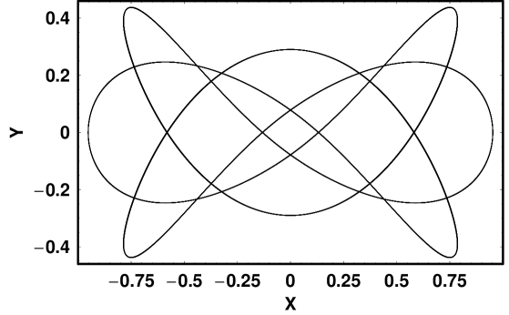
(e)

(f)

(g)

(h)

(i)

(j)

Figure 5: (a)–(j): Ten typical orbits in the global Hamiltonian (2) when $E_{\rm J}=-2700$.

Let us now proceed in order to study the behavior of the orbits, in the global model, near the galactic center, that is close to the nuclear region. In order to visualize the nature of motion near the nuclear region of our dynamical system, we present Figure 4 which shows the $x-p_{x}$, $y=0$, $p_{y}>0$ phase plane when $E_{\rm J}=-2700$. Once more, the particular value of the energy $E_{\rm J}$ was chosen so that in the phase plane $x_{\rm max}\simeq 1$. One observes a very interesting and complicated phase plane with regions of regular motion and a large, unified chaotic domain. In fact, there are two main regular regions consisting of invariant curves that are topological circles enclosing the two stable invariant points. The two stable invariant points $D$ and $R$ represent the direct (i.e. in the same direction as the rotation) and the retrograde periodic orbits respectively. These periodic orbits are characteristic of the 1:1 resonance and are similar to ellipses circulating around the origin. The rest of the regular region consists of several sets of smaller islands of invariant curves produced by quasi-periodic orbits belonging to resonances of higher multiplicity. The chaotic domain shown in the phase plane of Figure 4 consists of a large, unified chaotic sea and sticky regions. It is well known that the phenomenon of stickiness is common in barred galaxies (see Caranicolas & Karanis 1998; Karanis & Caranicolas 2002). The outermost curve shown in the phase plane of Figure 4 is the limiting curve defined by $H(x,p_{x})=E_{\rm J}$.

Comparing the present results with those given in Paper P1, we understand that the presence of the massive nucleus dramatically changes the nature of motion in our barred galactic model. In Paper P1, the motion was regular and there was only one kind of invariant curve. The invariant curves were topological circles closing around the unique central invariant point. The corresponding orbits were box orbits. The outer invariant curves belonged to elongated box orbits that support the bar, but as we approached the central invariant point, the box orbits became more rectangular (see fig. 4 of Paper P1 for more details). On the other hand, in the present case, we have resonant periodic or quasi-periodic orbits producing several sets of islands of invariant curves. Furthermore, the majority of the phase plane shown in Figure 4 is covered by chaotic orbits. We will return to this point later in the discussion.

Figure 5(a)–(j) shows ten typical orbits of the Hamiltonian system, when $E_{\rm J}=-2700$. Figure 5(a) shows a periodic orbit starting at the position of the direct stable invariant point. This orbit produces an invariant curve which belongs to the main set of invariant curves and encloses the fixed direct invariant point. The initial conditions are: $x_{0}=-0.363$, $y_{0}=0$, $p_{x0}=0$. In Figure 5(b) we see a typical example of a 1:2 resonant periodic orbit, which produces the set of the invariant curves close to the limiting curve. This orbit has initial conditions: $x_{0}=0.51$, $y_{0}=0$, $p_{x0}=32.8$. The orbit shown in Figure 5(c) produces the set of two small islands of invariant curves embedded near the main set of invariant curves around the retrograde stable point. This orbit represents the 2:2 resonance and has initial conditions: $x_{0}=0.152$, $y_{0}=0$, $p_{x0}=0$. The orbit depicted in Figure 5(d) produces one of the islands of invariant curves that intersects the $p_{x}$ axis. The initial conditions are: $x_{0}=0.018$, $y_{0}=0$, $p_{x0}=38.6$. In Figure 5(e) we see a 3:4 resonant orbit with initial conditions: $x_{0}=0.0756$, $y_{0}=0$, $p_{x0}=24.5$. Figure 5(f) shows a periodic orbit characteristic of the 3:5 resonance and produces a set of five small islands of invariant curves embedded in the chaotic region. This orbit has initial conditions: $x_{0}=0.952$, $y_{0}=0$, $p_{x0}=0$. In Figure 5(g) one can observe a typical 5:5 resonant periodic orbit. This orbit produces the set of the five small islands around the invariant curves of the direct point and has initial conditions: $x_{0}=-0.609$, $y_{0}=0$, $p_{x0}=0$. Figure 5(h) shows a periodic orbit which belongs to the 5:7 resonance family and produces a set of seven small islands of invariant curves. The initial conditions are: $x_{0}=0.797,y_{0}=0,p_{x0}=0$. In Figure 5(i) we see a complicated periodic orbit characteristic of the 5:9 resonance, which produces a set of nine tiny islands embedded in the chaotic sea. The initial conditions of this orbit are: $x_{0}=1.025,y_{0}=0,p_{x0}=0$. Finally, in Figure 5(j) we see a chaotic orbit with initial conditions: $x_{0}=0.71,y_{0}=0,p_{x0}=0$. The initial value of $p_{y0}$ was found in every case from the Jacobi integral (2). All orbits shown in Figure 5(a)–(j) were calculated for a time period of 100 time units.

We have to point out that the nature of the local motion near the central region of the galaxy is much more complicated than the global motion. This can be justified by the fact that the phase plane shown in Figure 4 which corresponds to the local motion contains more resonant cases than the phase plane of the global motion, which is shown in Figure 2. Therefore, we may conclude that the presence of a massive nucleus near the galactic center gives rise to a large variety of resonant orbits of higher multiplicity.

3 Properties of motion in the local model

The local potential can be found by expanding the effective potential (3) in a Taylor series near the central stable Lagrange point $L_{1}$, which coincides with the origin. Following this procedure and keeping only terms up to the fourth degree in the variables, we obtain the local effective potential which is

$$U_{\rm eff}\left(\Delta x,\Delta y\right) = U_{\rm eff}(0,0)+\frac{1}{2}\left[A\left(\Delta x\right)^{2}+B\left(\Delta y\right)^{2}\right]$$ (8)

$$-\frac{1}{4}\left[\alpha_{1}\left(\Delta x\right)^{4}+2\alpha_{2}\left(\Delta x\right)^{2}\left(\Delta y\right)^{2}+\alpha_{3}\left(\Delta y\right)^{4}\right]$$

$$-\frac{1}{2}\Omega_{0}^{2}\left[\left(\Delta x\right)^{2}+\left(\Delta y\right)^{2}\right],$$

where we have set

$$U_{\rm eff}=\frac{\alpha c_{\rm n}^{2}}{M_{\rm d}}\Phi_{\rm eff},$$ (9)

in order to avoid large numbers. Setting for convenience: $x=\Delta x$, $y=\Delta y$ and $V_{\rm eff}=U_{\rm eff}-U_{\rm eff}(0,0)$, Equation (8) becomes

$$V_{\rm eff}(x,y)=\frac{1}{2}\left(Ax^{2}+By^{2}\right)-\frac{1}{4}\left(\alpha_{1}x^{4}+2\alpha_{2}x^{2}y^{2}+\alpha_{3}y^{4}\right)-\frac{1}{2}\Omega_{0}^{2}\left(x^{2}+y^{2}\right),$$ (10)

where

$$A = \frac{c_{\rm n}^{2}}{\alpha^{2}}+\frac{\alpha c_{\rm n}^{2}M_{\rm b}}{M_{\rm d}c_{\rm b}^{3}}+\frac{\alpha M_{\rm n}}{M_{\rm d}c_{\rm n}}+\frac{\upsilon_{0}^{2}\alpha c_{\rm n}^{2}}{M_{\rm d}c_{\rm h}^{2}}\,,$$

$$B = \frac{c_{\rm n}^{2}}{\alpha^{2}}+\frac{\alpha b^{2}c_{\rm n}^{2}M_{\rm b}}{M_{\rm d}c_{\rm b}^{3}}+\frac{\alpha M_{\rm n}}{M_{\rm d}c_{\rm n}}+\frac{\upsilon_{0}^{2}\alpha\beta c_{\rm n}^{2}}{M_{\rm d}c_{\rm h}^{2}},$$

$$\alpha_{1} = \frac{3}{2}\left(\frac{c_{\rm n}^{2}}{\alpha^{4}}+\frac{\alpha M_{\rm b}}{M_{\rm d}c_{\rm b}^{5}}+\frac{\alpha M_{\rm n}}{M_{\rm d}c_{\rm n}^{3}}\right)+\frac{\upsilon_{0}^{2}\alpha c_{\rm n}^{2}}{M_{\rm d}c_{\rm h}^{4}}\,,$$

$$\alpha_{2} = \frac{3}{2}\left(\frac{c_{\rm n}^{2}}{\alpha^{4}}+\frac{\alpha b^{2}c_{\rm n}^{2}M_{\rm b}}{M_{\rm d}c_{\rm b}^{5}}+\frac{\alpha M_{\rm n}}{M_{\rm d}c_{\rm n}^{3}}\right)+\frac{\upsilon_{0}^{2}\alpha\beta c_{\rm n}^{2}}{M_{\rm d}c_{\rm h}^{4}},$$

$$\alpha_{3} = \frac{3}{2}\left(\frac{c_{\rm n}^{2}}{\alpha^{4}}+\frac{\alpha b^{4}c_{\rm n}^{2}M_{\rm b}}{M_{\rm d}c_{\rm b}^{5}}+\frac{\alpha M_{\rm n}}{M_{\rm d}c_{\rm n}^{3}}\right)+\frac{\upsilon_{0}^{2}\alpha\beta^{2}c_{\rm n}^{2}}{M_{\rm d}c_{\rm h}^{4}}\,,$$

$$\Omega_{0} = c_{\rm n}\Omega_{\rm b}\sqrt{\frac{\alpha}{M_{\rm d}}}\,.$$ (11)

As one can see from Equation (11), the coefficients of the local effective potential are functions of the physical quantities entering the global effective potential (3).

The local Hamiltonian is

$$H_{\rm L}=\frac{1}{2}\left(p_{x}^{2}+p_{y}^{2}\right)+V_{\rm eff}(x,y)=h_{\rm L}\,,$$ (12)

where $p_{x}$ and $p_{y}$ are the local momenta per unit mass, conjugate to $x$ and $y$ respectively, while $h_{\rm L}$ is the numerical value of the local energy.

In order to connect the value of the global energy $E_{\rm J}$ with the value of the local energy $h_{\rm L}$, we proceed as follows. The equation $E_{\rm J0}=\Phi_{\rm eff}(0,0)$ defines a point in the $\left(x,y\right)$ plane, while $E_{\rm J}=\Phi_{\rm eff}(x,y)$ defines a curve in the same plane. The global motion takes place inside this curve, which is known as the zero velocity curve. At the same time, $h_{\rm L0}=V_{\rm eff}(0,0)$ defines a point in the $\left(x,y\right)$ plane, while $h_{\rm L}=U_{\rm eff}(x,y)$ defines a curve inside which the local motion takes place. This second curve is the local zero velocity curve. We only consider bounded motion, which means the zero velocity curves are always closed. The local energy $h_{\rm L}$ is connected to the global energy $E_{\rm J}$ through the relation

$$h_{\rm L} = U_{\rm eff}(x,y)-U_{\rm eff}(0,0)=\frac{\alpha c_{\rm n}^{2}}{M_{\rm d}}\left[\Phi_{\rm eff}(x,y)-\Phi_{\rm eff}(0,0)\right]$$ (13)

$$= \frac{\alpha c_{\rm n}^{2}}{M_{\rm d}}\left(E_{\rm J}-E_{\rm J0}\right),$$

where

$$E_{\rm J0}=-\left(\frac{M_{\rm d}}{\alpha}+\frac{M_{\rm b}}{c_{\rm b}}+\frac{M_{\rm n}}{c_{\rm n}}\right)+\upsilon_{0}^{2}\ln\left(c_{\rm h}\right).$$ (14)

Let us now study the properties of the local motion. For the adopted values of the global parameters and for $\Omega_{\rm b}=1.25$, we find that: $A=1.4,B=1.5,\alpha_{1}=32.8,\alpha_{2}=32.4,\alpha_{3}=32.8$ and $\Omega_{0}=0.009$. For the value of the global energy $E_{\rm J}=-2700$ we find, by using Equation (13), that $h_{\rm L}=0.08452$. It is amazing that this value of the local energy is much larger than the energy of escape for the corresponding local potential (see Caranicolas & Varvoglis 1984; Caranicolas & Karanis 1998), which is given by

$$h_{\rm esc}=\frac{\left(B-\Omega_{0}^{2}\right)^{2}}{6\alpha_{1}}\,.$$ (15)

For the above values of the parameters, Equation (15) gives the value $h_{\rm esc}=0.01196$. This value is less than $h_{\rm L}/7$. Therefore, one may conclude that near the massive nucleus we do not have local motion, or equivalently local orbits escape the nuclear region, because they possess a high value of local energy. In order to obtain an idea regarding the nature of the local motion near the nucleus, we must go to very low values of energies, that is when $h\ll h_{\rm L}$, where $h$ is the value of the energy.

Figure 6: The $x-p_{x}$ Poincaré phase plane for the local Hamiltonian (12), when $h=0.012$.

(a)

(b)

(c)

(d)

Figure 7: (a)–(d): Four typical orbits in the local Hamiltonian (12), when $h=0.012$.

Figure 6 shows the $x-p_{x}$, $y=0$, $p_{y}>0$ Poincaré phase plane when $h=0.012$. The motion is regular and the phase plane has all the characteristics of the 1:1 resonance. There are two stable invariant points marked as $D$ and $R$ corresponding to direct and retrograde resonant periodic orbits respectively. The unstable periodic point gives an orbit, which in the absence of rotation is the $p_{x}$ axis. Thus, we observe that the local motion near the nucleus consists of a low energy 1:1 resonant periodic orbit. Moreover, as the entire phase plane is covered with invariant curves corresponding only to regular orbits, we conclude that near the nucleus we do not observe any kind of local chaotic motion. This situation is completely different from that displayed in Paper P1, where the nucleus was not present. In that case, all orbits in the local potential were box orbits, without any resonance phenomena.

Figure 7(a)–(d) shows four orbits of the local Hamiltonian (12). Figure 7(a) and (b) show two periodic orbits starting at the direct and the retrograde periodic points respectively. The initial conditions for the orbit shown in Figure 7(a) are: $x_{0}=-0.0845$, $y_{0}=0$, $p_{x0}=0$, while for the orbit shown in Figure 7(b) are: $x_{0}=0.0885$, $y_{0}=0$, $p_{x0}=0$. In Figure 7(c) we observe an orbit starting at the unstable periodic point with initial conditions: $x_{0}=-0.0119$, $y_{0}=0$, $p_{x0}=0$. Finally, in Figure 7(d) we see a box orbit which produces one of the outer invariant curves shown in the phase plane of Figure 6. The initial conditions for this orbit are: $x_{0}=0.1425$, $y_{0}=0$, $p_{x0}=0$. The initial value of $p_{y0}$ was found in every case from the energy integral (12). All orbits shown in Figure 7(a)–(d) were calculated for a time period of 100 time units.

We must clarify to the reader that the Taylor expansion (10) is only valid when

$$\frac{x^{2}+y^{2}}{\alpha^{2}}\ll 1,\qquad\frac{x^{2}+b^{2}y^{2}}{c_{\rm b}^{2}}\ll 1,\qquad\frac{x^{2}+y^{2}}{c_{\rm n}^{2}}\ll 1,\qquad\frac{x^{2}+\beta y^{2}}{c_{\rm h}^{2}}\ll 1.$$ (16)

It is also important to note that, for a given value of the global energy $E_{\rm J}$, a corresponding value of the local energy $h_{\rm L}$ can be obtained through relation (13). It is obvious that this value of the local energy does not have any physical meaning if all the relations (16) are not satisfied.

In order to better estimate the degree of chaos displayed by the chaotic orbits shown in Figures 2 and 4, we decided to compute the maximum Lyapunov Characteristic Exponent (L.C.E.) (for details see Lichtenberg & Lieberman 1992). The results are shown in Figure 8. The curve labeled $G$ shows the evolution of the L.C.E. for a chaotic orbit with initial conditions in the chaotic region of Figure 2. The particular values of the initial conditions of this orbit are as in Figure 3(f). On the other hand, the curve labeled $L$ shows the evolution of the L.C.E. for a chaotic orbit with initial conditions in the chaotic region of Figure 4. The particular values of the initial conditions of this orbit are as in Figure 5(j). We observe that the value of the L.C.E. corresponding to the local system of Figure 4 is about ten times the value of the L.C.E. corresponding to the global system of Figure 2. Therefore, one can say that in this case we have not only fast chaos (see Caranicolas & Vozikis 1987), where the L.C.E. was on the order of unity, but also very fast chaos where the L.C.E. is about three times larger. It is evident that this is an indication of strong nuclear activity near the vicinity of the galactic center.

Figure 8: Time evolution of the L.C.E. for two chaotic orbits. The curve labeled $G$ corresponds to an orbit in the chaotic domain of the phase plane of Fig. 2, while the curve labeled $L$ corresponds to an orbit in the chaotic domain of the phase plane of Fig. 4.

4 Discussion and conclusions

One of the most important approaches in order to understand and reveal the dynamical behavior of a galactic system is based on the knowledge of the chaotic versus ordered nature of orbits. In the present research, we tried to achieve this using a global and a local potential describing a barred galaxy with a massive nucleus, a disk and prolate halo components. The corresponding local potential was found by expanding the global potential around the central stable Lagrange point, which coincides with the origin, in a Taylor series and keeping only terms up to the fourth degree in the variables. This local potential is a potential made up of a two-dimensional perturbed harmonic oscillator. The study of the motion in those potentials has been an active field of research over the last decades (see for examples Saitô & Ichimura 1979; Innanen 1985; Caranicolas 1984, 1994, 2000; Caranicolas & Karanis 1999; Caranicolas & Vozikis 2002). In later years, the study of the properties of motion in those dynamical systems has been explored in detail, using precise and modern analytical (see Elipe 2000, 2001; Elipe & Deprit 1999) or numerical (see Lara et al. 1999; Karanis & Caranicolas 2002) methods.

As expected, the local parameters and the corresponding local energy are functions of all the involved global parameters and the global energy. Our numerical experiments, in the global dynamical system for high values of the energy, suggest that more than $62\%$ of the tested orbits are chaotic. Comparing the outcomes with those of Paper P1 we see that, in the present case, we have a sharp increase of the total chaotic motion. It is evident that the chaotic domain in Figure 2 is much more extended. This means that the additional nucleus affects not only the region near the center of the galaxy, but also areas far from it. Another interesting observation is that the presence of the nucleus does not seem to affect the figure-eight quasi-periodic orbits, which are the building blocks of the barred structure of the galaxy. This result agrees with recent observations made by the Hubble Space Telescope, which revealed that a number of Seyfert galaxies display strong nuclear barred structure (see Regan & Mulchaey 1999). On the other hand, the global motion near the massive nucleus has the characteristic of a 1:1 resonance. Furthermore, the chaotic domain seems to be larger than that observed in Figure 2. This is natural because of the presence of the nearby massive nucleus. All the above results are completely different from the corresponding results obtained in Paper P1, where the motion was regular and all the orbits in the global system near the galactic center were box orbits.

The effect of a central mass concentration (CMC) on the phase space of global galactic models has already been studied extensively in several earlier research works (see Caranicolas & Zotos 2011; Zotos 2012). Hasan & Norman (1990) have shown that a black hole or a CMC in a barred galaxy can dissolve the barred structure. Moreover, the fundamental orbits of the system (called B orbits), supporting the bar, are orbits elongated in the direction of the bar. As the black hole’s mass increases, an inner Lindblad resonance (ILR) appears and moves outward. Thus, the B orbits disappear when the ILR reaches the end of the bar. This effect is significantly increased if the bar is thinner. Orbits that stay closer to the central mass, with smaller Jacobi constants, can change their character from regular to chaotic more easily. Furthermore, the study of Hasan et al. (1993) indicates that, as the mass of the CMC increases, the stable regular orbits in the region where the bar potential competes in strength with the central mass potential, especially around the region of the ILR, will no longer be present and their position will be occupied by chaotic orbits. Shen & Sellwood (2004) have conducted a systematic study of the effects of CMC on bars, using high quality $N$-body simulations. They have experimented with both strong and weak initial bars and a wide range of the physical parameters of the CMC, such as the final mass, the scale length and the mass growth time. Their outcomes suggest that, for a given mass, compact CMCs (such as super-massive black holes) are more destructive to barred structures than are more diffuse ones (such as molecular gas clouds in many galactic centers). They have shown that the former are more efficient scatterers of bars supporting regular elongated orbits, that pass close to the galactic center and, therefore, decrease the percentage of the regular orbits and increase the area of the chaotic region in the phase space. All the above research outcomes are in agreement with the present findings, which strongly indicate that the massive nucleus is a very important parameter of the dynamical system, since it is responsible not only for the chaotic motion of low energy stars but also for the several resonant orbits of higher multiplicity that appear in the local model. In particular, Figures 2 and 4 in the current paper remarkably resemble the Poincaré surface of section plots in figure 11 of Shen & Sellwood (2004), where a realistic self-consistent barred model was adopted.

Let us now consider the local motion. The local potential (10) has all the characteristics of the 1:1 resonance. Such potentials are known as perturbed elliptic oscillators (see Deprit 1991). It is very interesting that for the corresponding local energy given by Equation (13), the local motion is not bounded. In order to obtain bounded motion, one must approach very low values of local energies. Strictly speaking, the presence of the massive nucleus makes the local energy increase dramatically, so that considering all the zero velocity curves results in unbounded local motion. For values of local energies slightly lower than the value of the energy of escape, we observe resonance phenomena, namely the 1:1 resonant periodic orbits. Extensive numerical calculations in the local potential suggest that chaotic motion was not observed.

Bearing all the above in mind, we can say that this situation is entirely different from that investigated in Paper P1, where the properties of local motion were the same as those of the global motion near the galactic center (see figs. 4 and 5 in Paper P1). In our case, the corresponding local motion does not appear to exist and only very low energy local motion seems to be present. Furthermore, the fact that the corresponding value of the L.C.E., which was computed in the chaotic domain near the nuclear region, is much larger than unity suggests that there is a particular and strong activity in the central parts of galaxies with strong nuclear bars.

We consider this paper to be an initial effort in order to explore and reveal the dynamical structure of the system in more detail. As the present results are positive, further investigation will be initiated to study all the available phase space. Moreover, our gravitational model will be suitably modified, in order to be able to describe the properties of motion in a Hamiltonian galactic system of three degrees of freedom.