Saddle stresses for generic theories with a preferred acceleration scale

Abstract

We show how scaling arguments may be used to generate templates for the tidal stresses around saddles for a vast class of MONDian theories detached from their obligations as dark matter alternatives. Such theories are to be seen simply as alternative theories of gravity with a preferred acceleration scale, and could be tested in the solar system by extending the LISA Pathfinder (LPF) mission. The constraints thus obtained may then be combined, if one wishes, with requirements arising from astrophysical and cosmological applications, but a clear separation of the issues is achieved. The central technical content of this paper is the derivation of a scaling prescription allowing complex numerical work to be bypassed in the generation of templates. We find that LPF could constrain very tightly the acceleration $a_{0}$ and the free parameter $\kappa$ present in these theories. As an application of our technique we also produce predictions for the moon saddle (for which a similar scaling argument is applicable) with the result that we recommend that it should be included in orbit design.

I Introduction

There is an ubiquitous acceleration scale in the universe, $a_{0}\sim 10^{-10}\;\mathrm{ms}^{-2}$, which turns up variously in cosmology and astrophysics: the cosmic expansion rate, galactic rotation curves, etc. This observation has prompted the investigation of alternative theories of gravity endowed with a preferred acceleration. TeVeS Bekenstein (2005), and more generally relativistic MONDian theories Sanders (2005); Zlosnik et al. (2006, 2007); Milgrom (2009, 2010), provide a blueprint for such constructions. MONDian theories were first proposed with the motivation of bypassing the need for dark matter Milgrom (1983); Famaey and McGaugh (2011). However, they may also be considered independently from this application, and be seen simply as alternative theories of gravity Clifton et al. (2012) into which an acceleration scale has been embedded. In this guise they constitute prime targets for experimental gravitational tests inside the solar system.

As an example let us consider TeVeS (but what follows applies generally to what in Magueijo and Mozaffari (2012) was labelled “Type I” theories). Abstracting from aspects which do not affect the non-relativistic limit, the theory benefits from the leeway of a whole free-function $\mu$. Its choice may be informed by minimalism and simplicity, e.g. $\mu$ may be built to encode only 2, rather than 3 or more regimes. Putting aside details affecting the transition between the two regimes, we are then left with two free parameters: $a_{0}$ (the acceleration scale of the theory) and $\kappa$ (controlling the renormalization of the gravitational constant $G$). These are fixed by astrophysical and cosmological applications, if the theory is to act as a competitor to dark matter. But $a_{0}$ and $\kappa$ can also be seen as fully free parameters in any solar system test.

Specifically, these theories predict a rich phenomenology around the saddle points of the gravitational potential. The prospect of extending the LISA Pathfinder mission so that a saddle of the Sun-Earth-Moon system is visited brings them within experimental striking range Magueijo and Mozaffari (2012); Bevis et al. (2010); Bekenstein and Magueijo (2006); Trenkel et al. (2010); A. Mozaffari (2011); Galianni et al. (2011). Predictions for minimal theories constrained by cosmological and astrophysical applications were studied in Magueijo and Mozaffari (2012), where the general impact of a negative result was also examined. Detaching the target theory from its duties as “dark matter” alternative requires the generation of a large database of templates. However, re-running the adaptive-mesh code presented in Bevis et al. (2010) for each $\mu$ is simply not feasible, and we run up against a computational wall.

In this paper we show how this work can be partly alleviated. As long as we are interested in changing only $\kappa$ and $a_{0}$, a simple scaling argument allows the generation of the whole set of required templates from those obtained with fiducial values for $a_{0}$ and $\kappa$, shortcutting tedious or downright impossible hard labour. The analytical argument is laid down in Section II, and its application to LPF is given in Section III. In order to include another topical application, in Section IV we also show how the lunar saddle would fare, were LPF to include it in a mission extension.

II Scaling behaviour around saddles

Scaling is an interesting tool for generating solutions to apparently intractable problems. For example imposing a self-similar ansatz leads to striking progress in the study of gravitational collapse, rendering what a priori are PDEs into simpler ODEs (e.g. Bertschinger (1985a, b)). Scaling behaviour was observed in the MONDian tidal stresses around saddles, when comparing the profiles around the Moon saddle and the Earth-Sun saddle (see Fig. 12 in Bevis et al. (2010), and its surrounding comments). It was noted that the tidal stresses are very approximately the same once they are spatially stretched and their amplitude scaled to account for the different Newtonian tidal stress $A$. In what follows we rigorously explain this empirical fact and extend its scope, deriving the scaling laws associated with varying $a_{0}$ and $\kappa$.

In TeVeS and other type I theories Magueijo and Mozaffari (2012) the non-relativistic dynamics results from the joint action of the usual Newtonian potential $\Phi_{N}$ (associated with the metric) and a “fifth force” scalar field, $\phi$, responsible for MONDian effects. The total potential acting on non-relativistic particles is their sum $\Phi=\Phi_{N}+\phi$. The field $\phi$ is ruled by a non-linear Poisson equation:

$$\nabla\cdot\left(\mu(z)\nabla\phi\right)=\kappa G\rho,$$ (1)

with $z=\frac{\kappa}{4\pi}\frac{|\nabla\phi|}{a_{0}}$. Here $\kappa$ is a dimensionless constant and $a_{0}$ is the usual MONDian acceleration.

For these theories, the argument presented in Sections II and IV of Bekenstein and Magueijo (2006), for a specific $\mu$, can be generalized for any $\mu$. It is always possible to define a variable:

$$\mathbf{U}=-\frac{\kappa}{4\pi a_{0}}\mu(z)\nabla\phi$$ (2)

in terms of which the vacuum equations become:

$$\nabla\cdot\mathbf{U}=0$$ (3)

$$\alpha(U)\,U^{2}\,\nabla\wedge\mathbf{U}+\mathbf{U}\wedge\nabla U^{2}=0,$$ (4)

i.e. the free parameters $a_{0}$ and $\kappa$ drop out, and “universal” equations are obtained. Here

$$\alpha(U)=\frac{d\ln U^{2}}{d\ln\mu}\;,$$ (5)

(notice that $U^{2}=z^{2}\mu^{2}(z)$, so that $\mu$ can be written as a function of $U$ alone, $\mu=\mu(U)$). The MONDian physical force can be obtained from $\mathbf{U}$ using:

$$\mathbf{F}_{\phi}=-\nabla\phi={4\pi a_{0}\over k}\frac{1}{\mu(U)}\mathbf{U}\;,$$ (6)

which follows directly from (2). In Bekenstein and Magueijo (2006) the choice was made:

$$\mu=\frac{U^{1/2}}{(1+U^{2})^{1/4}}$$ (7)

so that $\alpha=4(1+U^{2})$, in agreement with Eqns. (30)-(31) of Bekenstein and Magueijo (2006), and

$$\mathbf{F}_{\phi}=-\nabla\phi={4\pi a_{0}\over k}(1+U^{2})^{1/4}{\mathbf{U}\over U^{1/2}}\,,$$ (8)

in agreement with Eqn. 32 in Bekenstein and Magueijo (2006). However, as we see, the argument can be adapted to any function $\mu$.

Equations (3) and (4) are invariant under a rigid rescaling of the spatial variables:

$$\mathbf{U} \rightarrow \mathbf{U}$$ (9)

$$\mathbf{x} \rightarrow \lambda\mathbf{x}$$ (10)

where $\lambda$ is spatially constant. To use the technical term they admit homothetic solutions, i.e.:

$$\mathbf{U}=\mathbf{F}(\lambda\mathbf{x})\;.$$ (11)

where $\mathbf{F}$ is a universal function. However, we have yet to supply Equations (3) and (4) with boundary conditions. This is done by going far enough from the saddle so that the field $\phi$ has entered the Newtonian regime. With the conventions used in Magueijo and Mozaffari (2012) one has $\mu\rightarrow 1$ (the renormalization in $G$ is fully absorbed in $\kappa$), and so:

$$\phi\approx\frac{\kappa}{4\pi}\Phi_{N}\;.$$ (12)

The appropriate boundary condition is then supplied from the Newtonian limit relation:

$$\mathbf{U}\approx\frac{\kappa}{4\pi a_{0}}\mathbf{F}_{\phi}\approx{\left(\frac{\kappa}{4\pi}\right)}^{2}\frac{1}{a_{0}}\mathbf{F}_{N}\;.$$ (13)

Let us first assume that we can approximate the Newtonian field around the saddle as a linear function, for the purpose of effectuating this matching. Then:

$${\mathbf{F}}_{N}=-\nabla\Phi_{N}=Ar{\mathbf{N}}(\theta,\phi),$$ (14)

where $A$ is the Newtonian tidal stress at the saddle point, and $\mathbf{N}$ is its angular profile (see Eqs. 35-37 in Bekenstein and Magueijo (2006)). Defining the MONDian “bubble size” as usual:

$$r_{0}=\frac{16\pi^{2}a_{0}}{\kappa^{2}A}$$ (15)

we therefore have in the Newtonian regime and close enough to the saddle:

$$\mathbf{U}\approx\frac{r}{r_{0}}\mathbf{N}(\theta,\phi)\;.$$ (16)

This boundary condition allows us to select the homothetic solution (11) appropriate to a given saddle and free parameters. To match the boundary conditions one should set $\lambda=1/r_{0}$, so that the solution is

$$\mathbf{U}=\mathbf{F}{\left(\frac{\mathbf{x}}{r_{0}}\right)}\;.$$ (17)

The above argument is still (approximately) valid if one goes beyond the linear approximation, as long as this approximation is good up to a few $r_{0}$. If the parameters $a_{0}$ and $\kappa$ lead to a breakdown of this assumption, however, then scaling is lost.

We can now read off similar scaling laws for more familiar quantities. Using (8) we see that the MONDian force must have the form:

$$\mathbf{F}_{\phi}=\frac{a_{0}}{\kappa}{\mathbf{G}}{\left(\frac{\mathbf{x}}{r_{0}}\right)}$$ (18)

where $\mathbf{G}$ is another universal function. (This scaling law is obvious by direct inspection of the analytical solutions derived for the $\mu$ used in Bekenstein and Magueijo (2006); however, as we now see, it is more general). By taking derivatives we then find that the MONDian tidal stresses must have the form

$$S_{ij}=\kappa AH_{ij}{\left(\frac{\mathbf{x}}{r_{0}}\right)}$$ (19)

where the $H_{ij}$ are also universal. This explains the scaling law observed for different $A$, and fixed $\kappa$ and $a_{0}$, when comparing the Moon and Earth saddles Bevis et al. (2010). But it also allows for templates for general values of $\kappa$ and $a_{0}$ to be generated from those for fiducial values simply by rescaling them according to the above laws.

III An application

The practical applications of the previous section are far-reaching and will be the subject of a number of future publications devoted to the data analysis of a saddle test. As a simple example we examine in this section the impact of $a_{0}$ and $\kappa$ on the SNR (Signal to Noise Ratio) forecast for a LISA Pathfinder flyby. As in Magueijo and Mozaffari (2012), we assume the use of an optimal noise-matched filter, using for our noise model the best estimate at the time of writing (labelled “Best Case Noise” in Fig.6 of Magueijo and Mozaffari (2012)). We then inspect the SNR variations with $a_{0}$ and $\kappa$ for different saddle impact parameters $b$. After a number of studies, following on from Trenkel et al. (2010), an impact parameter $b\sim 10-50\;\mathrm{km}$ is now considered realistic. Multiple flybys are currently being investigated, for which $b$ may not be as good. We therefore consider SNRs for $b$ up to 1000 km. Recall that for the fiducial values $a_{0}=10^{-10}\;\mathrm{ms}^{-2}$ and $\kappa=0.03$ (required, or suggested, by cosmological and astrophysical applications) one forecasts SNRs for the Earth-Sun saddle around 40-60 for the expected $b=10-50\;\mathrm{km}$, only dropping below 5 beyond $b\sim 700\;\mathrm{km}$ (see Fig.7 of Magueijo and Mozaffari (2012)).

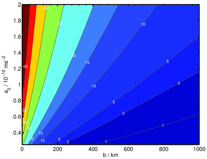
Figure 1: The effect on the Signal-to-Noise Ratio (SNR) resulting from varying $a_{0}$, assuming different impact parameters $b$ and the best estimate for the noise at the time of writing (with $\kappa$ kept fixed at $\kappa=0.03$). The fiducial value used in previous publications is $a_{0}=10^{-10}\;\mathrm{ms}^{-2}$. Generally the larger the $a_{0}$ the higher the SNR.

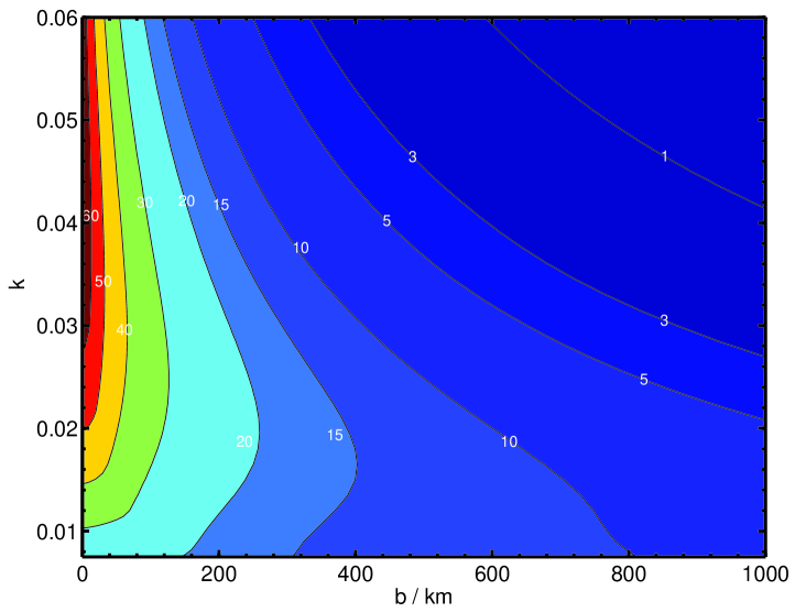
Figure 2: Effect on the SNR obtained by varying $\kappa$ (keeping $a_{0}$ fixed at the fiducial value). The fiducial value used in previous publications is $\kappa=0.03$. At small $b$, changing $\kappa$ may increase or decrease the SNR (see text for explanation). At large $b$ one is better off with a small $\kappa$.

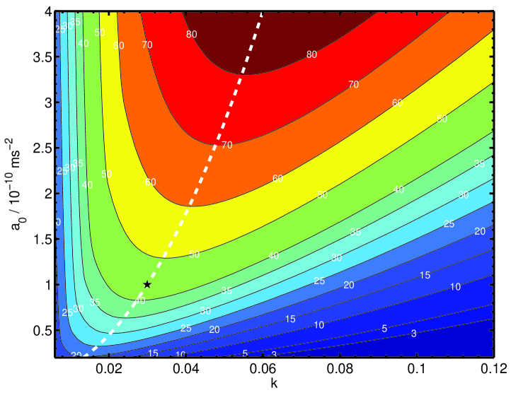
Figure 3: Effect on SNR obtained by jointly varying $a_{0}$ and $\kappa$, for a trajectory with impact parameter $b=50$km. The fiducial values have been indicated with a star. We also plot (dashed white line) the contour of constant $r_{0}$ passing through the fiducial values.

The effect of changing the acceleration scale $a_{0}$ is plotted in Fig. 1. It results from a change in the MOND bubble size $r_{0}$, as predicted by Eqn. 15. Therefore the SNR is roughly constant on lines of constant $b/a_{0}$. The slope of the iso-SNR lines is not constant and they are not exactly straight because the SNR algorithm is quite complicated and non-linear. We see that even at large $b$ it is possible to turn a weak result into a strong positive one by increasing $a_{0}$ by a factor of 2. Conversely, if $a_{0}$ is halved, a SNR below $\sim 5$ is now a liability for $b$ as low as $\sim 350\;\mathrm{km}$. Without external constraints fixing $a_{0}$ to better than an order of magnitude, it is therefore risky to give up on a $b\sim 10-50\;\mathrm{km}$.

The effect of changing $\kappa$ is plotted in Fig. 2 and results from two sources: a change in bubble size according to $r_{0}\propto 1/\kappa^{2}$ (cf. Eqn. 15) and an overall factor multiplying the amplitude (cf. Eqn. 19). The two effects counteract each other, so that unless $b$ is very large, the SNR at first increases with $\kappa$, then decreases. For the expected $b\sim 10-50$ it can go either way. For large $b$ (greater than $b\sim 500\;\mathrm{km}$ for the fiducial value of $a_{0}$), the bubble size prevails and so the SNR decreases with increasing $\kappa$. The interplay of these two effects is best illustrated in Fig. 3, where we plotted the effect on the SNR of changing simultaneously $a_{0}$ and $\kappa$ for fixed $b=50\;\mathrm{km}$. We also plotted the line of constant $r_{0}$ passing through the fiducial values. As we see the SNR does change along this line, showing that the bubble size $r_{0}$ is not the only consideration.

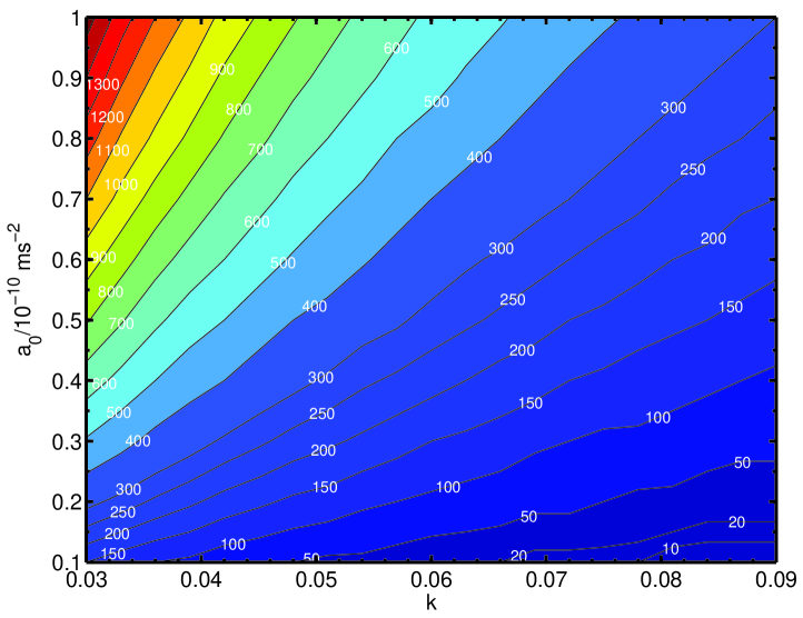
Figure 4: Constraints placed on $a_{0}$ and $\kappa$ by a negative result for different impact parameters $b$ (labelling the lines and coding the colours). For a given $b$, the admissible parameter space would be “outside” the corresponding $b$ line (i.e. towards the right lower corner).

Supposing we get a negative result, what constraints can we place upon $a_{0}$ and $\kappa$? As in Magueijo and Mozaffari (2012) we may get a preliminary estimate by seeking the region where the SNR for an optimal filter drops below 1. This was plotted Fig. 4 for various values of $b$ (in this figure, $b$ labels the lines and codes the colours). For a given $b$, the admissible parameter space is “outside” the corresponding $b$ line (i.e. towards the right-bottom corner). In general, a negative result forces $a_{0}$ to be smaller and $\kappa$ to be larger than the fiducial values, the more so, the smaller the impact parameter $b$. As we see, if we were to miss the saddle by 1500 km or more, the fiducial values of $a_{0}$ and $\kappa$ would survive a negative result. For an approach any closer, however, a negative result would rule them out and squeeze the parameter space towards the right-bottom corner. For $b\sim 10\;\mathrm{km}$, the $a_{0}$ (the $\kappa$) would have to be smaller (larger) than the fiducial values by an order of magnitude.

These constraints may now be combined with other pressures upon the theory, such as those arising from limits on $G$ renormalisation, Big Bang Nucleosynthesis, fifth force solar system tests, galaxy rotation curve data, and cosmological structure formation. However, as advocated in the introduction, by allowing complete freedom in $a_{0}$ and $\kappa$ in a saddle test, we have achieved a clear separation of the issues confronting these theories.

IV The moon saddle as a LPF target

Our technique can also be applied to a very topical issue: whether the Moon saddle is a good alternative target for LPF. Practical matters may render this saddle more amenable to multiple flybys, an issue that could be essential in dismissing a “false alarm”, should a positive detection be found. In the absence of a more detailed study of transfer orbits we evaluate SNR’s for the moon saddle, hoping that this may motivate further work in orbit design.

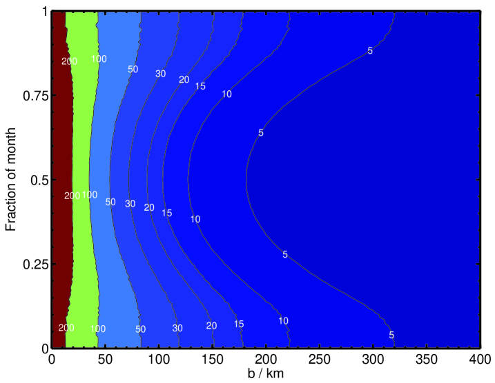
Figure 5: SNRs for the moon saddle, assuming a standard noise model and speed $v=0.3\;\mathrm{km}\;\mathrm{s}^{-1}$, for different impact parameters and day of the month (0 and 1 represent the New Moon, 0.5 the Full Moon). We see that the moon saddle is less forgiving if you miss it by more than 150 km and more rewarding if you get close to it (with SNRs of 200 within reach). If the former, new moons generate higher SNRs.

Application of the algorithm in Section II to the moon saddle is straightforward (and indeed it motivated the argument presented therein). As noted in Bevis et al. (2010), $r_{0}$ for the Moon saddle is smaller than the 380km found for the Earth-Sun saddle, and this size is more variable, depending strongly on the phase of the Moon (it varies between 25km and 80km; see Fig.10 of Bevis et al. (2010)). However $A$ is larger, too, so the tidal stresses have a larger amplitude. Nevertheless, what really matters for SNRs is the Fourier transform of the signal as seen in time, with the satellite going through the bubble. The large SNRs obtained for the Sun-Earth saddle result from a miraculous coincidence between the sweet spot in the amplitude spectral density (ASD), and the size of the bubble as transformed into a time-signal by the typical velocities found in transfer orbits. This miracle could be spoiled by the smaller size of the Moon saddle.

As it happens, orbits crossing the Moon saddle do so with a smaller velocity, typically smaller than $0.5\;\mathrm{km}\;\mathrm{s}^{-1}$. The two effects—smaller bubble, smaller speed—counteract each other when converting the bubble signal into a time signal. Therefore it is not surprising that the SNRs predicted for the Moon saddle are as high as those for the Earth saddle, albeit more variable in time, depending on the phase of the moon.

In Fig. 5 we plotted SNRs assuming the standard noise model we have used throughout this paper, for a crossing of the moon saddle at $v=0.3\;\mathrm{km}\;\mathrm{s}^{-1}$, for different impact parameters and day of the month. On the $y$- axis 0 and 1 represent the New Moon, and 0.5 represents the Full Moon. As we can see, in comparison with the Earth-Sun saddle, the moon saddle:

• is less forgiving if you miss it by more than 150 km.

• is more rewarding if you get close to it (with SNRs of 200 within reach).

• in the first case, then the lunar phase is crucial, with the new moon producing the best results.

In view of these results we think we should urge the orbit designers to include the moon saddle in their considerations.

V Conclusions

To conclude, we have presented a simple argument allowing the inference of a large database of templates for the tidal stresses that would be felt by LISA Pathfinder, should a saddle flyby be incorporated into the mission. The argument allows for the variation of the acceleration scale $a_{0}$ and $\kappa$. Should the functional form of the free function $\mu$ be changed, the SNRs obtained would change, but only as predicted in Magueijo and Mozaffari (2012): they wouldn’t change much for MONDian two-regime functions, unless $b$ is much larger than $r_{0}$. We may detach these theories altogether from their “alternative to dark matter duties”. Then we may consider two-regime functions with $\mu\rightarrow 1$ at large arguments, but $\mu\propto z^{n}$, with $n\neq 1$, when $z$ is small. The scaling argument presented here would still be applicable in this context, but the fiducial templates would have to be obtained by re-running a numerical code for each $n$. In a paper in preparation we show how this may be bypassed too, albeit with a much more complex analytical argument.

The practical applications of our technique are far-reaching and will be the support of a number of future publications concerned with the data analysis of a saddle test. In this paper we merely showed how SNRs change by changing the parameters of the theory. This gives an indication of how sensitive to them the experiment is, and therefore how much it will constrain them. More importantly, as an application we applied our scaling algorithm to the prediction of results for the Moon saddle. The results were very encouraging and lead us to urge the orbit designers to include it in their considerations.