Finite Size Scaling for the Glass Transition: the Role of a Static Length Scale
Abstract
Over the last decade computer simulations have had an increasing role in shedding light on difficult statistical physical phenomena and in particular on the ubiquitous problem of the glass transition. Here in a wide variety of materials the viscosity of a super-cooled liquid increases by many orders of magnitude upon decreasing the temperature over a modest range. A natural concern in these computer simulation is the very small size of the simulated systems compared to experimental ones, raising the issue of how to assess the thermodynamic limit. Here we offer a theory for the glass transition based on finite size scaling, a method that was found very useful in the context of critical phenomena and other interesting problems. As is known, the construction of such a theory rests crucially on the existence of a growing static length scale upon decreasing the temperature. We demonstrate that the static length scale that was discovered in Ref. 12KLP fits the bill extremely well, allowing us to provide a finite size scaling theory for the relaxation time of the glass transition, including predictions for the thermodynamic limit based on simulations in small systems.
I Introduction
Glasses are ubiquitous in nature; the problem of the glass transition where the viscosity of a super-cooled liquid increases by many orders of magnitude upon a temperature decrease of a couple of hundred degrees remains one of the major challenges in modern condensed matter physics. With the advent of powerful computers, numerical simulations played a vital role in revealing some of the crucial characteristic associated with this phenomenon 09Cav ; 11BB . In spite of this progress, due to still present limitations in computer power, simulations are still done in small sample sizes from thousands to a few tens of thousands of particles. Compared to experimental samples this is minute. Thus finite size effects in the results are always a major concern, especially when one deals with a system where a characteristic length scale grows with decreasing temperature 12KLP .
Finite size effects are not always unwanted; in fact one can extract useful insights by studying these effects carefully 90B . As an example the temperature dependence of the static length scale can be obtained from the system size dependence of some relevant observable by analyzing the data using finite size scaling. In the glass community the existence and usefulness of a static length scale is still debated; even if one can extract some static length scale by doing some sophisticated analysis 03Ber ; 08BBCGV ; 09KDS , the slow growth of this length scale makes it difficult to extract reliable insights . Nevertheless finite size effects in the dynamics of the supercooled liquids certainly exist, notwithstanding the fact that the characteristic length scale may not change very much. A careful analysis of these effects can shed a substantial light on the physics of the glass transition 91DIRP ; 98DDPPG ; 00KY ; 00FP ; 01BKB ; 02DFPG ; 03Ber ; 09KDS ; 10KDS ; 10KDSa ; 10RRH ; 96Horbach ; 99BH ; 03DH .
In 12KLP , we already showed that our proposed length scale is the same object which governs the finite size effects exhibited in configurational entropy in the Kob-Andersen Model in 3 dimensions 09KDS . Further more and are related via the empirical Adam-Gibbs relation AG or may be via more sophisticated RFOT Theory RFOT ; RFOT1 ; RFOT2 . So our length scale directly relates dynamics with thermodynamics in glass forming liquids via the Adam-Gibbs relation. Unfortunately we can not determine the exponents predicted in the RFOT Theory since the range of increase of our length scale is not sufficient to determine reliably the exponents.
In this study our main aim is to establish that our proposed length scale is a crucial object for the theory of glass transition by demonstrating that it faithfully explains the finite size effects seen in relaxation times. In a similar attempt in 10RRH to explain the finite size effect seen in the relaxation time, it was argued that a large system of particles can be thought of as a collection of smaller subsystems called “elementary units” which are coupled to each other by coupling constants. The finite size effects seen in the relaxation times can be thought of as a organized rearrangements of these elementary units. It is quite possible that our proposed length scale actually measures the size of these elementary units, but further study is needed to pinpoint this connection. It is also worth mentioning that in 10RRH a linear relationship has been proposed between the relaxation time and the system size for small system sizes. In contrast we propose a scaling function associated with the underlying growing static length scale.
A clear advantage of our proposed length scale 12KLP is that it is relatively easy to extract both in simulations and in experiments 10GCSKB as compared to the other length scales like point-to-set 08BBCGV and patch length scale 11KL ; 11SL . While we can compute our length scale for larger range of temperature this is prohibitive for the other length scales, thus at this time there is not enough data to provide a conclusive comparison between these length scales.
Below we present a systematic study of the system size dependence of the -relaxation time of different model glass forming systems in both two and three dimensions. We choose two completely different interaction pair potential- one with pure repulsion and one with short range repulsion and long range attraction to stress the generality of the finite size effects in the dynamics of glass forming systems 12BBCKT .
II Models and Methods
Here we study two distinct models, one with pure power law repulsive interaction 12KLP ; 11KLPZ and the second being the well-studied Kob-Andersen Model 95KA in both 2 and 3 dimensions. We will denote the Kob-Andersen Model in 3-dimensions as 3d KA and the slightly modified version of it for 2-dimensions as 2d mKA 09BSPK . The pure repulsive models will be referred to as 3d R10 and 2d R10 for 3-dimensions and 2-dimensions respectively. The usual Kob-Andersen model with a binary mixture in 2-dimension shows prominent clustering effects so the model was slightly modified and a binary mixture was used. This modified model shows no clustering behavior in all the simulated temperature range 09BSPK ; 12SKDS . Throughout this paper we use temperature units such that the Boltzmann constant equals unity.
The potential of the Kob-Andersen model is given by
| (1) |
where and , , , , , . The Interaction Potential was cut off at 2.50. We have performed the simulations at six different temperatures in the range in 3-dimensions and in 2-dimensions at a number density .
The interaction potential for the pure repulsive model is given by
| (2) |
where is the distance between particle and , is the energy scale, and is the dimensionless length for which the potential vanishes continuously with derivatives. The interaction length scale between any two particles and is , and for two ‘small’ particles, one ‘large’ and one ‘small’ particle and two ‘large’ particle respectively. The coefficients are given by
| (3) |
We chose the parameters , and . The unit of length is set to be the interaction length scale of two small particles, and is the unit of energy. We have performed the simulations at six different temperatures in range at number density in 3-dimensions and at for 2-dimensions.
We have simulated these models in the ensemble using a Berendsen thermostat 84BPGDH to maintain the temperature. The system size was in the range and we used as many as to different samples to average the data depending on the system size. Generally for small system sizes and at low temperature the fluctuations increase, demanding more extensive averaging of the data to get reliable estimates of the wanted observables. For each system size and each temperature we measured the -relaxation time and the characteristic length scale. The former is calculated from the decay of the overlap correlation function defined as
| (4) |
where the weight function if and zero otherwise. The -relaxation time is the time where this correlation function goes to of its initial value i.e. . The characteristic length scale was measured using the method proposed in Ref. 12KLP . The reader is encouraged to examine this reference for the details of the method. In brief, it is based on the insight that the minimum eigenvalue of the Hessian matrix belongs to either an elastic mode or to a plastic mode, depending on the system size. The characteristic length is the crossover system size between these two possibilities. The Hessian matrix is obtained for every supercooled system at temperature by employing the conjugate gradient minimization methods to get an inherent structure (at temperature ), and then using the Lanczos method lancAlgo to get the minimum eigenvalue.
III Results

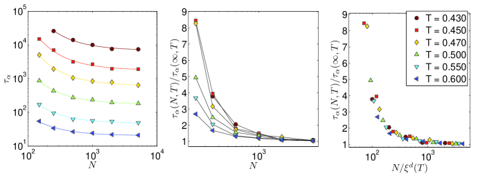
In the left panel of Fig.1, we present the system size dependence of the -relaxation time for the Kob-Andersen model in 3-dimensions, for different temperatures. The data indicates a substantial system size dependence of the relaxation time which appears to increase slowly with decreasing the temperature. This is an indication that the length scale which governs this behavior increases also with decreasing the temperature. Physically we expect the relaxation time to decrease with increasing system size if one asserts the existence of a cooperative length scale. This length scale becomes relevant to the system’s dynamics when the temperature goes bellow the so-called ‘onset temperature’ 01sastry which separates the characteristic Arrhenius regime from the ‘fragile’ regime of the temperature dependence of the relaxation time, cf. 12HKPZ . The argument is as follows : For a system of size at temperature , the typical free energy barrier it needs to cross for relaxation is
| (5) |
where is the potential energy barrier. We expect the potential barrier to be determined by the energy landscape which in general does not depend on the system size. On the other hand is the entropic contribution to the free energy barrier. Now at temperatures lower than the onset temperature 01sastry the cooperative relaxation mechanism plays the main role for relaxation and one expects the degeneracy factor for this case to be system size dependent when the system size is small.
Consider a system of particles in a cubic box of size at some temperature . In the non-Arrhenius regime with a typical length , we expect for a system with , that any relaxation event will occur on the scale in order to be successful. So the degeneracy factor will grow with system size. For a system with we expect without any change when the system size grows. Thus the free energy barrier can be represented as a scaling function of according to
| (6) |
where is a proportionality constant independent of the temperature, and obviously
| (7) |
Next we calculate the system size dependence of the relaxation time for different temperatures, using the estimate where is a typical attempt time, cf. 12HKPZ . The result is again a scaling function of , reading
| (8) | |||||
From the property (7) of the scaling function we confirm that when .
Examine the consequences of these arguments for the data of the Kob-Andersen model, cf Fig. 1. In the left panel we present the relaxation time for different temperatures and systems sizes. In the middle panel of Fig.1 we rescaled the y-axis by the large value of of the relaxation time for the different temperatures. We estimated this value by fitting the data with a functional form ; One sees that this fitting is adequate for obtaining the large value of the relaxation time. In the right panel of Fig.1, we present the full data collapse which is obtained by rescaling the system size using the length scale obtained in 12KLP . We stress that no adjustments were necessary and none were made to these length scales, they were employed as obtained. Now one may ask whether a similar collapse can be done using the other static length scales mentioned above. In a recent study 12HMR it was shown that the point-to-set length scale in the Kob-Andersen model in three dimension changes by a factor of in the temperature range . Assuming that we can extrapolate these data to lower temperature we find point-to-set length scale changes by similar factor in the temperature range of our study. Thus it appears possible to collapse the relaxation time data using the point-to-set length scale in this temperature range. This suggests that point-to-set length scale is proportional to our length scale. It remains a future work to compute point-to-set length scale to lower temperature to confirm this connection.
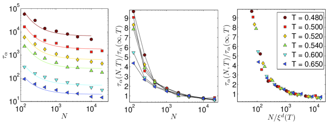
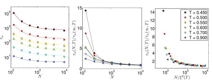
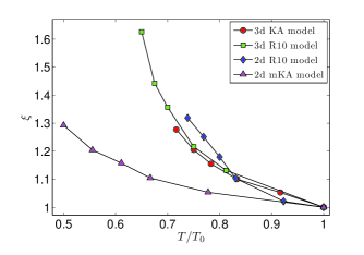
In Fig.4 we present the results of a similar analysis for the model system with pure repulsive interaction (3d R10) in 3-dimensions. The data collapse observed in the right panel is again quite good. We present similar analysis in 2-dimensions for the model with pure repulsive interaction in Fig.4 and for the modified Kob-Andersen model in Fig.4. In Fig.6, we plotted the temperature dependence of the correlation length for all the models studied to compare the model to model variation of the growth of this length scale with decreasing temperature.
IV Universal Relation Between and
Having found that the typical scale fits the bill for finite size scaling, we should ask next whether there is a direct, and possibly universal relation, between the length scale and the time scale. We start with the following ansatz for the relation between structural relaxation time in the thermodynamic limit and the static correlation length .
| (9) |
where is a non-universal coefficient that depends on the details of the glass former. To set a scale to this relation we choose a reference temperature where the typical length is . Then the relaxation time at that temperature is
| (10) |
So we have the following relation
| (11) | |||||
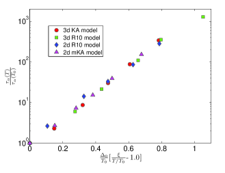
We reiterate that in the above equation the pre-factor is not known apriori for different models. In Fig.6 we plotted the relaxation time data according to Eq.11, with ,and for KA model in 3D, R10 model in 3D, R10 model in 2D and modified KA model in 2D respectively. We choose for all the models. The collapse of the data indicates an encouraging possible universal relation between the static length scale and the relaxation time.
To conclude, we have studied the finite size effects in the dynamics of supercooled liquids for different models systems in both 2 and 3 dimensions. In this article we have focused on the system size dependence of the -relaxation time and found that the finite size effects can be very well explained by the static length scale that we proposed in 12KLP for all these different models. In a recent study 12BBCKT , it was argued that a growing static length scale is necessary to explain the finite size effects seen in the simulational studies of model glass forming liquids. We want to stress that our proposed length scale 12KLP is indeed that length scale which faithfully explains all the finite size effects seen in the simulation results.
Further more we realized that there is a possibility of universal relation between this length scale and the -relaxation time when relaxation time for different models are plotted as a function of the length scales, all the data fall nicely on a master curve as also recently reported in 12HMR . This connection again seems to suggest that point-to-set length scale might be proportional to our proposed length scale. We reiterate that further study is needed to confirm this relation and care should be taken as these length scales and the relaxation times are not varying by much in the temperature range for which we could do the simulations. We hope that our work will inspire other researchers to do further studies to delineate, especially in the low temperature range, the validity of this apparent universal behaviour between the relaxation time and the static length scale.
Acknowledgements.
This work had been supported in part by an advanced “ideas” grant of the European Research Council, the Israel Science Foundation and the German Israeli Foundation. We thank Shiladitya Sengupta, JNCASR, Bangalore for many useful discussions.References
- (1) A. Cavagna Phys. Rep. 476, 51 (2009).
- (2) L. Berthier and G. Biroli, Rev. Mod. Phys. 83, 587-645 (2011).
- (3) S. Karmakar, E. Lerner, I. Procaccia, Physica A , 391, 1001 (2012)
- (4) K. Binder , Z Phys B 43, 119 –140 (1990).
- (5) G. Biroli, J.-P. Bouchaud, A. Cavagna, T. S. Grigera,and P. Verrochio, Nature Phys. 4, 771 (2008).
- (6) L. Berthier, Phys. Rev. Lett. 91, 055701-1 (2003).
- (7) S. Karmakar, C. Dasgupta and S. Sastry, Proc. Natl. Acad. Sci. U.S.A. 106, 3675 (2009).
- (8) C. Dasgupta, A.V. Indrani, S. Ramaswamy, M.K. Phani, Europhys Lett 15, 307–312 (1991).
- (9) C. Donati, J.F. Douglas, S.J. Plimpton, P.H. Poole, S.C. Glotzer, Phys Rev Lett 80, 2338 (1998).
- (10) K. Kim and R. Yamamoto, Phys Rev E 61, R41 (2000).
- (11) S. Franz, G. Parisi, J. Phys. Condens. Matter. 12, 6335 (2000).
- (12) C. Brangian, W. Kob, K. Binder, Europhys Lett 53, 756 (2001).
- (13) C. Donati, F. Franz, G. Parisi, S.C. Glotzer, J. Non-Cryst. Solids. 307, 215 (2002).
- (14) S. Karmakar, C. Dasgupta and S. Sastry, Phys. Rev. Lett. 105, 015701 (2010).
- (15) S. Karmakar, C. Dasgupta and S. Sastry, Phys. Rev. Lett. 105, 019801 (2010).
- (16) C. Rehwald, O. Rubner, and A. Heuer, Phys. Rev. Lett. 105, 117801 (2010).
- (17) J. Horbach et al., Phys. Rev. E 54, R5897 (1996).
- (18) S. Buchner and A. Heuer, Phys. Rev. E 60, 6507 (1999).
- (19) D. Doliwa and A. Heuer, J. Phys.: Condens. Matter 15 S849 (2003).
- (20) G. Adams and J.H. Gibbs, J. Chem. Phys. 43, 139 (1965).
- (21) T.R. Kirkpatrick, D. Thirumalai, P.G. Wolynes, Phys Rev A 40, 1045 (1989).
- (22) V. Lubchenko, P.G. Wolynes, Annu Rev Phys Chem 58, 235 (2007).
- (23) G. Biroli and J.-P. Bouchaud, Structural Glasses and Supercooled Liquids: Theory, Experiment, and Applications - edited by P.G. Wolynes, V. Lubchenko, John Wiley & Sons, (2012).
- (24) A. Ghosh, V. K. Chikkari, P. Schall, J. Kurchan and D. Bonn Phys. Rev. Lett., 104, 248305 (2010).
- (25) J. Kurchan and D. Levine, J. Phys. A: Math. Theor. 44, 035001 (2011).
- (26) F. Sausset and D. Levine, Phys. Rev. Lett. 107, 045501 (2011).
- (27) L. Berthier, et. al - arXiv.1203.3392 preprint 2012.
- (28) S. Karmakar, E. Lerner, I. Procaccia and J. Zylberg, Phys. Rev. E 83, 046106 (2011).
- (29) W. Kob and H. C. Andersen, Phys. Rev. E 51, 4626 (1995).
- (30) R. Bruning, D.A. St-Onge, S. Patterson, W. Kob, J. Phys.: Condens. Matter 21 035117, (2009).
- (31) S. Sengupta, S. Karmakar, C. Dasgupta, and S. Sastry (unpublished).
- (32) H.J.C. Berendsen, J.P.M. Postma, W.F. van Gunsteren, A. Dinola, and J.R. Haak, J. Chem. Phys. 81, 3684 (1984).
- (33) http://en.wikipedia.org/wiki/Lanczos_algorithm.
- (34) H.G.E. Hentschel, S. Karmakar, I. Procaccia and J. Zylberg, - arXiv:1202.1127 preprint 2012.
- (35) S. Sastry, Nature 409, 164 (2001).
- (36) G.M. Hocky, T.E. Markland, D.R. Reichman - Phys. Rev. Lett. 108, 225506 (2012).