The Deodhar decomposition of the Grassmannian and the regularity of KP solitons

Abstract.

Given a point $A$ in the real Grassmannian, it is well-known that one can construct a soliton solution $u_{A}(x,y,t)$ to the KP equation. The contour plot of such a solution provides a tropical approximation to the solution when the variables $x$, $y$, and $t$ are considered on a large scale and the time $t$ is fixed. In this paper we use several decompositions of the Grassmannian in order to gain an understanding of the contour plots of the corresponding soliton solutions. First we use the positroid stratification of the real Grassmannian in order to characterize the unbounded line-solitons in the contour plots at $y\gg 0$ and $y\ll 0$. Next we use the Deodhar decomposition of the Grassmannian – a refinement of the positroid stratification – to study contour plots at $t\ll 0$. More specifically, we index the components of the Deodhar decomposition of the Grassmannian by certain tableaux which we call Go-diagrams, and then use these Go-diagrams to characterize the contour plots of solitons solutions when $t\ll 0$. Finally we use these results to show that a soliton solution $u_{A}(x,y,t)$ is regular for all times $t$ if and only if $A$ comes from the totally non-negative part of the Grassmannian.

1. Introduction

The KP equation is a two-dimensional nonlinear dispersive wave equation which was proposed by Kadomtsev and Peviashvili in 1970 to study the stability problem of the soliton solution of the Korteweg-de Vries (KdV) equation [14]. The KP equation can also be used to describe shallow water waves, and in particular, the equation provides an excellent model for the resonant interaction of those waves. The equation has a rich mathematical structure, and is now considered to be the prototype of an integrable nonlinear dispersive wave equation with two spatial dimensions (see for example [26, 1, 10, 25, 13]).

One of the main breakthroughs in the KP theory was given by Sato [31], who realized that solutions of the KP equation could be written in terms of points on an infinite-dimensional Grassmannian. The present paper deals with a real, finite-dimensional version of the Sato theory; in particular, we are interested in solutions that are localized along certain rays in the $xy$ plane called line-solitons. Such a soliton solution can be constructed from a point $A$ of the real Grassmannian. More specifically, one can apply the Wronskian form [31, 32, 12, 13] to $A$ to produce a $\tau$-function $\tau_{A}(x,y,t)$ which is a sum of exponentials, and from the $\tau$-function one can construct a solution $u_{A}(x,y,t)$ to the KP equation.

Recently several authors have studied the soliton solutions $u_{A}(x,y,t)$ which come from points $A$ of the totally non-negative part of the Grassmannian $(Gr_{k,n})_{\geq 0}$, that is, those points of the real Grassmannian $Gr_{k,n}$ whose Plücker coordinates are all non-negative [3, 18, 2, 5, 7, 20, 21]. These solutions are regular, and include a large variety of soliton solutions which were previously overlooked by those using the Hirota method of a perturbation expansion [13].

One of the main goals of this paper is to understand the soliton solutions $u_{A}(x,y,t)$ coming from arbitrary points $A$ of the real Grassmannian, not just the totally non-negative part. In general such solutions are no longer regular – they may have singularities along rays in the $xy$ plane – but it is possible, nevertheless, to understand a great deal about the asymptotics of such solutions.

Towards this end, we use two related decompositions of the real Grassmannian. The first decomposition is Postnikov’s positroid stratification of the Grassmannian [28], whose strata are indexed by various combinatorial objects including decorated permutations and $\Gamma$ -diagrams. Note that the intersection of each positroid stratum with $(Gr_{k,n})_{\geq 0}$ is a cell (homeomorphic to an open ball); when one intersects the positroid stratification of the Grassmannian with the totally non-negative part, one obtains a cell decomposition of $(Gr_{k,n})_{\geq 0}$ [28].

The second decomposition is the Deodhar decomposition of the Grassmannian, which is a refinement of the positroid stratification. Its components have explicit parameterizations due to Marsh and Rietsch [24], and are indexed by distinguished subexpressions of reduced words in the Weyl group. The components may also be indexed by certain tableaux filled with black and white stones which we call Go-diagrams, and which provide a generalization of $\Gamma$ -diagrams. Note that almost all Deodhar components have an empty intersection with the totally non-negative part of the Grassmannian. More specifically, each positroid stratum is a union of Deodhar components, precisely one of which has a non-empty intersection with $(Gr_{k,n})_{\geq 0}$.

By using the positroid stratification of the Grassmannian, we characterize the unbounded line-solitons of KP soliton solutions coming from arbitrary points of the real Grassmannian. More specifically, given $A\in Gr_{k,n}$, we show that the unbounded line-solitons of the solution $u_{A}(x,y,t)$ at $y\ll 0$ and $y\gg 0$ depend only on which positroid stratum $A$ belongs to, and that one can use the corresponding decorated permutation to read off the unbounded line-solitons. This extends work of [2, 5, 7, 20, 21] from the setting of the non-negative part of the Grassmannian to the entire real Grassmannian.

By using the Deodhar decomposition of the Grassmannian, we give an explicit description of the contour plots of soliton solutions in the $xy$-plane when $t\ll 0$. The contour plot of the solution $u_{A}(x,y,t)$ at a fixed $t$ approximates the locus where $|u_{A}(x,y,t)|$ takes on its maximum values or is singular. More specifically, we provide an algorithm for constructing the contour plot of $u_{A}(x,y,t)$ at $t\ll 0$, which uses the Go-diagram indexing the Deodhar component of $A$. We also show that when the Go-diagram $D$ is a $\Gamma$ -diagram, then the corresponding contour plot at $t\ll 0$ gives rise to a positivity test for the Deodhar component $S_{D}$.

Finally we use our previous results to address the regularity problem for KP solitons. We prove that a soliton solution $u_{A}(x,y,t)$ coming from a point $A$ of the real Grassmannian is regular for all times $t$ if and only if $A$ is a point of the totally non-negative part of the Grassmannian.

The structure of this paper is as follows. In Section 2 we provide background on the Grassmannian and some of its decompositions, including the positroid stratification. In Section 3 we describe the Deodhar decomposition of the complete flag variety and its projection to the Grassmannian, while in Section 4 we explain how to index Deodhar components in the Grassmannian by Go-diagrams (Subsection 4.2). In Section 5 we provide explicit formulas for certain Plücker coordinates of points in Deodhar components (Theorems 5.2 and 5.6), and use these formulas to provide positivity tests for points in the real Grassmannian (Theorem 5.13). Subsequent sections provide applications of the previous results to soliton solutions of the KP equation. In Section 6 we give background on how to produce a soliton solution to the KP equation from a point of the real Grassmannian. In Section 7 we define the contour plot associated to a soliton solution at a fixed time $t$ (Definition 7.1), then in Section 8 we use the positroid stratification to describe the unbounded line-solitons in contour plots of soliton solutions at $y\gg 0$ and $y\ll 0$ (Theorem 8.1). In Section 9 we define the more combinatorial notions of soliton graph and generalized plabic graph. In Section 10 we use the Deodhar decomposition to describe contour plots of soliton solutions for $t\ll 0$ (Theorem 10.6), and in Section 11 we provide some technical results on $X$-crossings in contour plots and corresponding relations among Plücker coordinates. Finally we use the results of the previous sections to address the regularity problem for soliton solutions in Section 12 (Theorem 12.1).

2. Background on the Grassmannian and its decompositions

The real Grassmannian $Gr_{k,n}$ is the space of all $k$-dimensional subspaces of $\mathbb{R}^{n}$. An element of $Gr_{k,n}$ can be viewed as a full-rank $k\times n$ matrix modulo left multiplication by nonsingular $k\times k$ matrices. In other words, two $k\times n$ matrices represent the same point in $Gr_{k,n}$ if and only if they can be obtained from each other by row operations. Let $\binom{[n]}{k}$ be the set of all $k$-element subsets of $[n]:=\{1,\dots,n\}$. For $I\in\binom{[n]}{k}$, let $\Delta_{I}(A)$ be the Plücker coordinate, that is, the maximal minor of the $k\times n$ matrix $A$ located in the column set $I$. The map $A\mapsto(\Delta_{I}(A))$, where $I$ ranges over $\binom{[n]}{k}$, induces the Plücker embedding $Gr_{k,n}\hookrightarrow\mathbb{RP}^{\binom{n}{k}-1}$.

We now describe several useful decompositions of the Grassmannian: the matroid stratification, the Schubert decomposition, and the positroid stratification. Their relationship is as follows: the matroid stratification refines the positroid stratification which refines the Schubert decomposition. In Section 3.4 we will describe the Deodhar decomposition, which is a refinement of the positroid stratification, and (as verified in [35]) is refined by the matroid stratification.

2.1. The matroid stratification of $Gr_{k,n}$

Definition 2.1.

A matroid of rank $k$ on the set $[n]$ is a nonempty collection $\operatorname{\mathcal{M}}\subset\binom{[n]}{k}$ of $k$-element subsets in $[n]$, called bases of $\operatorname{\mathcal{M}}$, that satisfies the exchange axiom:
For any $I,J\in\operatorname{\mathcal{M}}$ and $i\in I$ there exists $j\in J$ such that $(I\setminus\{i\})\cup\{j\}\in\operatorname{\mathcal{M}}$.

Definition 2.2.

A loop of a matroid on the set $[n]$ is an element $i\in[n]$ which is in every basis. A coloop is an element $i\in[n]$ which is not in any basis.

Given an element $A\in Gr_{k,n}$, there is an associated matroid $\operatorname{\mathcal{M}}_{A}$ whose bases are the $k$-subsets $I\subset[n]$ such that $\Delta_{I}(A)\neq 0$.

Definition 2.3.

Let $\operatorname{\mathcal{M}}\subset\binom{[n]}{k}$ be a matroid. The matroid stratum $S_{\operatorname{\mathcal{M}}}$ is defined to be

$$S_{\operatorname{\mathcal{M}}}=\{A\in Gr_{k,n}\ |\ \Delta_{I}(A)\neq 0\text{ if and only if }I\in\operatorname{\mathcal{M}}\}.$$

This gives a stratification of $Gr_{k,n}$ called the matroid stratification, or Gelfand-Serganova stratification. The matroids $\operatorname{\mathcal{M}}$ with nonempty strata $S_{\operatorname{\mathcal{M}}}$ are called realizable over $\mathbb{R}$.

2.2. The Schubert decomposition of $Gr_{k,n}$

We now turn to the Schubert decomposition of the Grassmannian. First recall that the partitions $\lambda\subset(n-k)^{k}$ are in bijection with $k$-element subset $I\subset[n]$. The boundary of the Young diagram of such a partition $\lambda$ forms a lattice path from the upper-right corner to the lower-left corner of the rectangle $(n-k)^{k}$. Let us label the $n$ steps in this path by the numbers $1,\dots,n$, and define $I=I(\lambda)$ as the set of labels on the $k$ vertical steps in the path. Conversely, we let $\lambda(I)$ denote the partition corresponding to the subset $I$.

Definition 2.4.

For each partition $\lambda\subset(n-k)^{k}$, one can define the Schubert cell $\Omega_{\lambda}$ to be the set of all elements $A\in Gr_{k,n}$ such that when $A$ is represented by a matrix in row-echelon form, it has pivots precisely in the columns $I(\lambda)$. As $\lambda$ ranges over the partitions contained in $(n-k)^{k}$, this gives the Schubert decomposition of the Grassmannian $Gr_{k,n}$, i.e.

$$Gr_{k,n}=\bigsqcup_{\lambda\subset(n-k)^{k}}\,\Omega_{\lambda}.$$

Definition 2.5.

Let $\{i_{1},i_{2},\dots,i_{k}\}$ and $\{j_{1},j_{2},\dots,j_{k}\}$ be two $k$-element subsets of $\{1,2,\dots,n\}$, such that $i_{1}<i_{2}<\dots<i_{k}$ and $j_{1}<j_{2}<\dots<j_{k}$. We define the component-wise order $\preceq$ on $k$-element subsets of $\{1,2,\dots,n\}$ as follows:

$$\{i_{1},i_{2},\dots,i_{k}\}\preceq\{j_{1},j_{2},\dots,j_{k}\}\text{ if and only if }i_{1}\leq j_{1},i_{2}\leq j_{2},\dots,\text{ and }i_{k}\leq j_{k}.$$

Lemma 2.6.

Let $A$ be an element of the Schubert cell $\Omega_{\lambda}$, and let $I=I(\lambda)$. If $\Delta_{J}(A)\neq 0$, then $I\preceq J$. In particular,

$$\Omega_{\lambda}=\{A\in Gr_{k,n}\ |\ I(\lambda)\text{ is the lexicographically minimal base of }\operatorname{\mathcal{M}}_{A}\}.$$

Proof. This follows immediately by considering the representation of $A$ as a matrix in row-echelon form.        

We now define the shifted linear order $<_{i}$ (for $i\in[n]$) to be the total order on $[n]$ defined by

$$i<_{i}i+1<_{i}i+2<_{i}\dots<_{i}n<_{i}1<_{i}\dots<_{i}i-1.$$

One can then define cyclically shifted Schubert cells as follows.

Definition 2.7.

For each partition $\lambda\subset(n-k)^{k}$ and $i\in[n]$, we define the cyclically shifted Schubert cell $\Omega_{\lambda}^{i}$ by

$$\Omega_{\lambda}^{i}=\{A\in Gr_{k,n}\ |\ I(\lambda)\text{ is the lexicographically minimal base of }\operatorname{\mathcal{M}}_{A}\text{ with respect to }<_{i}\}.$$

Note that $\Omega_{\lambda}=\Omega_{\lambda}^{1}$.

2.3. The positroid stratification of $Gr_{k,n}$

The positroid stratification of the real Grassmannian $Gr_{k,n}$ is obtained by taking the simultaneous refinement of the $n$ Schubert decompositions with respect to the $n$ shifted linear orders $<_{i}$. This stratification was first considered by Postnikov [28], who showed that the strata are conveniently described in terms of Grassmann necklaces, as well as decorated permutations and $\Gamma$ -diagrams. Postnikov coined the terminology positroid because the intersection of the positroid stratification with the totally non-negative part of the Grassmannian $(Gr_{k,n})_{\geq 0}$ gives a cell decomposition of $(Gr_{k,n})_{\geq 0}$ (whose cells are called positroid cells).

Definition 2.8.

[28, Definition 16.1] A Grassmann necklace is a sequence $\operatorname{\mathcal{I}}=(I_{1},\dots,I_{n})$ of subsets $I_{r}\subset[n]$ such that, for $i\in[n]$, if $i\in I_{i}$ then $I_{i+1}=(I_{i}\setminus\{i\})\cup\{j\}$, for some $j\in[n]$; and if $i\notin I_{i}$ then $I_{i+1}=I_{i}$. (Here indices $i$ are taken modulo $n$.) In particular, we have $|I_{1}|=\dots=|I_{n}|$, which is equal to some $k\in[n]$. We then say that $\operatorname{\mathcal{I}}$ is a Grassmann necklace of type $(k,n)$.

Example 2.9.

$\mathcal{I}=(1257,2357,3457,4567,5678,6789,1789,1289,1259)$ is an example of a Grassmann necklace of type $(4,9)$.

Lemma 2.10.

[28, Lemma 16.3] Given $A\in Gr_{k,n}$, let $\mathcal{I}(A)=(I_{1},\dots,I_{n})$ be the sequence of subsets in $[n]$ such that, for $i\in[n]$, $I_{i}$ is the lexicographically minimal subset of $\binom{[n]}{k}$ with respect to the shifted linear order $<_{i}$ such that $\Delta_{I_{i}}(A)\neq 0$. Then $\operatorname{\mathcal{I}}(A)$ is a Grassmann necklace of type $(k,n)$.

If $A$ is in the matroid stratum $S_{\operatorname{\mathcal{M}}}$, we also use $\operatorname{\mathcal{I}}_{\operatorname{\mathcal{M}}}$ to denote the sequence $(I_{1},\dots,I_{n})$ defined above. This leads to the following description of the positroid stratification of $Gr_{k,n}$.

Definition 2.11.

Let $\operatorname{\mathcal{I}}=(I_{1},\dots,I_{n})$ be a Grassmann necklace of type $(k,n)$. The positroid stratum $S_{\operatorname{\mathcal{I}}}$ is defined to be

$$S_{\operatorname{\mathcal{I}}}=\{A\in Gr_{k,n}\ |\ \operatorname{\mathcal{I}}(A)=\operatorname{\mathcal{I}}\}.$$

Remark 2.12.

By comparing Definition 2.11 to Definition 2.7, we see that given a Grassmann necklace $\operatorname{\mathcal{I}}=(I_{1},\dots,I_{n})$,

$$S_{\operatorname{\mathcal{I}}}=\bigcap_{i=1}^{n}~{}\Omega_{\lambda(I_{i})}^{i}\,.$$

In other words, each positroid stratum is an intersection of $n$ cyclically shifted Schubert cells.

Definition 2.13.

[28, Definition 13.3] A decorated permutation $\pi^{:}=(\pi,col)$ is a permutation $\pi\in S_{n}$ together with a coloring function $col$ from the set of fixed points $\{i\ |\ \pi(i)=i\}$ to $\{1,-1\}$. So a decorated permutation is a permutation with fixed points colored in one of two colors. A weak excedance of $\pi^{:}$ is a pair $(i,\pi(i))$ such that either $\pi(i)>i$ or $\pi(i)=i$ and $col(i)=1$. We call $i$ the weak excedance position. If $\pi(i)>i$ (respectively $\pi(i)<i$) then $(i,\pi(i))$ is called an excedance (respectively, nonexcedance).

Example 2.14.

The decorated permutation (written in one-line notation) $(6,7,1,2,8,3,9,4,5)$ has no fixed points, and four weak excedances, in positions $1,2,5$ and $7$.

Definition 2.15.

[28, Definition 6.1] Fix $k$, $n$. If $\lambda$ is a partition, let $Y_{\lambda}$ denote its Young diagram. A $\Gamma$ -diagram $(\lambda,D)_{k,n}$ of type $(k,n)$ is a partition $\lambda$ contained in a $k\times(n-k)$ rectangle together with a filling $D:Y_{\lambda}\to\{0,+\}$ which has the $\Gamma$ -property: there is no $0$ which has a $+$ above it and a $+$ to its left. (Here, “above” means above and in the same column, and “to its left” means to the left and in the same row.)

In Figure 1 we give an example of a $\Gamma$ -diagram.

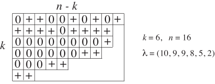
Figure 1. A Le-diagram $L=(\lambda,D)_{k,n}$.

We now review some of the bijections among these objects.

Definition 2.16.

[28, Section 16] Given a Grassmann necklace $\mathcal{I}$, define a decorated permutation $\pi^{:}=\pi^{:}(\mathcal{I})$ by requiring that

1. if $I_{i+1}=(I_{i}\setminus\{i\})\cup\{j\}$, for $j\neq i$, then $\pi(j)=i$.

2. if $I_{i+1}=I_{i}$ and $i\in I_{i}$ then $\pi(i)=i$ is colored with $col(i)=1$.

3. if $I_{i+1}=I_{i}$ and $i\notin I_{i}$ then $\pi(i)=i$ is colored with $col(i)=-1$.

As before, indices are taken modulo $n$.

If $\pi^{:}=\pi^{:}(\mathcal{I})$, then we also use the notation $S_{\pi^{:}}$ to refer to the positroid stratum $S_{\operatorname{\mathcal{I}}}$.

Example 2.17.

Definition 2.16 carries the Grassmann necklace of Example 2.9 to the decorated permutation of Example 2.14.

Lemma 2.18.

[28, Lemma 16.2] The map $\mathcal{I}\to\pi^{:}(\mathcal{I})$ is a bijection from Grassmann necklaces $\mathcal{I}=(I_{1},\dots,I_{n})$ of size $n$ to decorated permutations $\pi^{:}(\mathcal{I})$ of size $n$. Under this bijection, the weak excedances of $\pi^{:}(\mathcal{I})$ are in positions $I_{1}$.

Remark 2.19.

Use the notation of Lemma 2.18. It follows from the definition of the positroid stratification that if $A\in S_{\operatorname{\mathcal{I}}}$ is written in row-echelon form, then the pivots are located in position $I_{1}$. It follows from Lemma 2.18 that the pivot positions coincide with the weak excedance positions of $\pi^{:}(\operatorname{\mathcal{I}})$.

2.4. Irreducible elements of $Gr_{k,n}$

Definition 2.20.

We say that a full rank $k\times n$ matrix is irreducible if, after passing to its reduced row-echelon form $A$, the matrix $A$ has the following properties:

1. Each column of $A$ contains at least one nonzero element.

2. Each row of $A$ contains at least one nonzero element in addition to the pivot.

An irreducible Grassmann necklace of type $(k,n)$ is a sequence $\mathcal{I}=(I_{1},\dots,I_{n})$ of subsets $I_{r}$ of $[n]$ of size $k$ such that, for $i\in[n]$, $I_{i+1}=(I_{i}\setminus\{i\})\cup\{j\}$ for some $j\neq i$. (Here indices $i$ are taken modulo $n$.) A derangement $\pi=(\pi_{1},\dots,\pi_{n})$ is a permutation $\pi\in S_{n}$ which has no fixed points.

In the language of matroids, an element $A\in S_{\operatorname{\mathcal{M}}}$ is irreducible if and only if the matroid $\operatorname{\mathcal{M}}$ has no loops or coloops. It is easy to see that if $A$ is irreducible, then $\operatorname{\mathcal{I}}(A)$ is an irreducible Grassmann necklace and $\pi^{:}(\operatorname{\mathcal{I}})$ is a derangement.

3. Projecting the Deodhar decomposition of $G/B$ to the Grassmannian

In this section we review Deodhar’s decomposition of the flag variety $G/B$ [8]. By projecting it, one may obtain a decomposition of any partial flag variety $G/P$ (and in particular the Grassmannian), obtaining the decomposition which Deodhar described in [9]. We also review the parameterizations of the components due to Marsh and Rietsch [24].

3.1. The flag variety

The following definitions can be made for any split, connected, simply connected, semisimple algebraic group over a field ${\mathbb{K}}$. However this paper will be concerned with $G=\mathrm{SL}_{n}=\mathrm{SL}_{n}(\mathbb{R})$.

We fix a maximal torus $T$, and opposite Borel subgroups $B^{+}$ and $B^{-}$, which consist of the diagonal, upper-triangular, and lower-triangular matrices, respectively. We let $U^{+}$ and $U^{-}$ be the unipotent radicals of $B^{+}$ and $B^{-}$; these are the subgroups of upper-triangular and lower-triangular matrices with $1$’s on the diagonals. For each $1\leq i\leq n-1$ we have a homomorphism $\phi_{i}:{\rm SL}_{2}\to{\rm SL}_{n}$ such that

$$\phi_{i}\begin{pmatrix}a&b\\ c&d\end{pmatrix}=\begin{pmatrix}1&&&&&\\ &\ddots&&&&\\ &&a&b&&\\ &&c&d&&\\ &&&&\ddots&\\ &&&&&1\end{pmatrix}~{}\in{\rm SL}_{n},$$

that is, $\phi_{i}$ replaces a $2\times 2$ block of the identity matrix with $\begin{pmatrix}a&b\\ c&d\end{pmatrix}$. Here $a$ is at the $(i+1)$st diagonal entry counting from the southeast corner. We use this to construct $1$-parameter subgroups in $G$ (landing in $U^{+}$ and $U^{-}$, respectively) defined by

$$x_{i}(m)=\phi_{i}\left(\begin{array}[]{cc}1&m\\ 0&1\\ \end{array}\right)\text{ and }\ y_{i}(m)=\phi_{i}\left(\begin{array}[]{cc}1&0\\ m&1\\ \end{array}\right),\ \text{ where }m\in\mathbb{R}.$$

The datum $(T,B^{+},B^{-},x_{i},y_{i};i\in I)$ for $G$ is called a pinning.

Let $W$ denote the Weyl group $N_{G}(T)/T$, where $N_{G}(T)$ is the normalizer of $T$. The simple reflections $s_{i}\in W$ are given explicitly by $s_{i}:=\dot{s_{i}}T$ where $\dot{s_{i}}:=\phi_{i}\left(\begin{array}[]{cc}0&-1\\ 1&0\\ \end{array}\right)$ and any $w\in W$ can be expressed as a product $w=s_{i_{1}}s_{i_{2}}\dots s_{i_{m}}$ with $m=\ell(w)$ factors. We set $\dot{w}=\dot{s}_{i_{1}}\dot{s}_{i_{2}}\dots\dot{s}_{i_{m}}$. For $G=\mathrm{SL}_{n}$, we have $W={\mathfrak{S}}_{n}$, the symmetric group on $n$ letters, and $s_{i}$ is the transposition exchanging $i$ and $i+1$.

We can identify the flag variety $G/B$ with the variety $\mathcal{B}$ of Borel subgroups, via

$$gB\longleftrightarrow g\cdot B^{+}:=gB^{+}g^{-1}.$$

We have two opposite Bruhat decompositions of $\mathcal{B}$:

$$\mathcal{B}=\bigsqcup_{w\in W}B^{+}\dot{w}\cdot B^{+}=\bigsqcup_{v\in W}B^{-}\dot{v}\cdot B^{+}.$$

Note that $B^{-}\dot{v}\cdot B^{+}\cong\mathbb{R}^{\ell(w_{0})-\ell(v)}$. The closure relations for these opposite Bruhat cells are given by $B^{-}\dot{v}^{\prime}\cdot B^{+}\subset\overline{B^{-}\dot{v}\cdot B^{+}}$ if and only if $v\leq v^{\prime}$. We define

$$\mathcal{R}_{v,w}:=B^{+}\dot{w}\cdot B^{+}\cap B^{-}\dot{v}\cdot B^{+},$$

the intersection of opposite Bruhat cells. This intersection is empty unless $v\leq w$, in which case it is smooth of dimension $\ell(w)-\ell(v)$, see [16, 23]. The strata $\mathcal{R}_{v,w}$ are often called Richardson varieties.

3.2. Distinguished expressions

We now provide background on distinguished and positive distinguished subexpressions, as in [8] and [24]. We will assume that the reader is familiar with the (strong) Bruhat order $<$ on the Weyl group $W={\mathfrak{S}}_{n}$, and the basics of reduced expressions, as in [4].

Let $\mathbf{w}:=s_{i_{1}}\dots s_{i_{m}}$ be a reduced expression for $w\in W$. We define a subexpression $\mathbf{v}$ of $\mathbf{w}$ to be a word obtained from the reduced expression $\mathbf{w}$ by replacing some of the factors with $1$. For example, consider a reduced expression in ${\mathfrak{S}}_{4}$, say $s_{3}s_{2}s_{1}s_{3}s_{2}s_{3}$. Then $s_{3}s_{2}\,1\,s_{3}s_{2}\,1$ is a subexpression of $s_{3}s_{2}s_{1}s_{3}s_{2}s_{3}$. Given a subexpression $\mathbf{v}$, we set $v_{(k)}$ to be the product of the leftmost $k$ factors of $\mathbf{v}$, if $k\geq 1$, and $v_{(0)}=1$. The following definition was given in [24] and was implicit in [8].

Definition 3.1.

Given a subexpression $\mathbf{v}$ of a reduced expression $\mathbf{w}=s_{i_{1}}s_{i_{2}}\dots s_{i_{m}}$, we define

$$J^{\circ}_{\mathbf{v}} :=\{k\in\{1,\dotsc,m\}\ |\ v_{(k-1)}<v_{(k)}\},$$

$$J^{\Box}_{\mathbf{v}}\, :=\{k\in\{1,\dotsc,m\}\ |\ v_{(k-1)}=v_{(k)}\},$$

$$J^{\bullet}_{\mathbf{v}} :=\{k\in\{1,\dotsc,m\}\ |\ v_{(k-1)}>v_{(k)}\}.$$

The expression $\mathbf{v}$ is called non-decreasing if $v_{(j-1)}\leq v_{(j)}$ for all $j=1,\dotsc,m$, e.g. $J^{\bullet}_{\mathbf{v}}=\emptyset$.

The following definition is from [8, Definition 2.3]:

Definition 3.2 (Distinguished subexpressions).

A subexpression $\mathbf{v}$ of $\mathbf{w}$ is called distinguished if we have

(3.1) $$v_{(j)}\leq v_{(j-1)}\ s_{i_{j}}\qquad\text{for all $~{}j\in\{1,\dotsc,m\}$}.$$

In other words, if right multiplication by $s_{i_{j}}$ decreases the length of $v_{(j-1)}$, then in a distinguished subexpression we must have $v_{(j)}=v_{(j-1)}s_{i_{j}}$.

We write $\mathbf{v}\prec\mathbf{w}$ if $\mathbf{v}$ is a distinguished subexpression of $\mathbf{w}$.

Definition 3.3 (Positive distinguished subexpressions).

We call a subexpression $\mathbf{v}$ of $\mathbf{w}$ a positive distinguished subexpression (or a PDS for short) if

(3.2) $$v_{(j-1)}<v_{(j-1)}s_{i_{j}}\qquad\text{for all $~{}j\in\{1,\dotsc,m\}$}.$$

In other words, it is distinguished and non-decreasing.

Lemma 3.4.

[24] Given $v\leq w$ and a reduced expression $\mathbf{w}$ for $w$, there is a unique PDS $\mathbf{v}_{+}$ for $v$ in $\mathbf{w}$.

3.3. Deodhar components in the flag variety

We now describe the Deodhar decomposition of the flag variety. This is a further refinement of the decomposition of $G/B$ into Richardson varieties $\mathcal{R}_{v,w}$. Marsh and Rietsch [24] gave explicit parameterizations for each Deodhar component, identifying each one with a subset in the group.

Definition 3.5.

[24, Definition 5.1] Let $\mathbf{w}=s_{i_{1}}\dots s_{i_{m}}$ be a reduced expression for $w$, and let $\mathbf{v}$ be a distinguished subexpression. Define a subset $G_{\mathbf{v},\mathbf{w}}$ in $G$ by

(3.3) $$G_{\mathbf{v},\mathbf{w}}:=\left\{g=g_{1}g_{2}\cdots g_{m}\left|\begin{array}[]{ll}g_{\ell}=x_{i_{\ell}}(m_{\ell})\dot{s}_{i_{\ell}}^{-1}&\text{ if $\ell\in J^{\bullet}_{\mathbf{v}}$,}\\ g_{\ell}=y_{i_{\ell}}(p_{\ell})&\text{ if $\ell\in J^{\Box}_{\mathbf{v}}$,}\\ g_{\ell}=\dot{s}_{i_{\ell}}&\text{ if $\ell\in J^{\circ}_{\mathbf{v}}$,}\end{array}\quad\text{ for $p_{\ell}\in\mathbb{R}^{*},\,m_{\ell}\in\mathbb{R}$. }\right.\right\}.$$

There is an obvious map $(\mathbb{R}^{*})^{|J^{\Box}_{\mathbf{v}}|}\times\mathbb{R}^{|J^{\bullet}_{\mathbf{v}}|}\to G_{\mathbf{v},\mathbf{w}}$ defined by the parameters $p_{\ell}$ and $m_{\ell}$ in (3.3). For $v=w=1$ we define $G_{\mathbf{v},\mathbf{w}}=\{1\}$.

Example 3.6.

Let $W={\mathfrak{S}}_{5}$, $\mathbf{w}=s_{2}s_{3}s_{4}s_{1}s_{2}s_{3}$ and $\mathbf{v}=s_{2}111s_{2}1$. Then the corresponding element $g\in G_{\mathbf{v},\mathbf{w}}$ is given by $g=s_{2}y_{3}(p_{2})y_{4}(p_{3})y_{1}(p_{4})x_{2}(m_{5})s_{2}^{-1}y_{3}(p_{6})$, which is

$$g=\begin{pmatrix}1&0&0&0&0\\ p_{3}&1&0&0&0\\ 0&p_{6}&1&0&0\\ p_{2}p_{3}&p_{2}-m_{5}p_{6}&-m_{5}&1&0\\ 0&-p_{4}p_{6}&-p_{4}&0&1\end{pmatrix}.$$

The following result from [24] gives an explicit parametrization for the Deodhar component $\mathcal{R}_{\mathbf{v},\mathbf{w}}$. We will take the description below as the definition of $\mathcal{R}_{\mathbf{v},\mathbf{w}}$.

Proposition 3.7.

[24, Proposition 5.2] The map $(\mathbb{R}^{*})^{|J^{\Box}_{\mathbf{v}}|}\times\mathbb{R}^{|J^{\bullet}_{\mathbf{v}}|}\to G_{\mathbf{v},\mathbf{w}}$ from Definition 3.5 is an isomorphism. The set $G_{\mathbf{v},\mathbf{w}}$ lies in $U^{-}\dot{v}\cap B^{+}\dot{w}B^{+}$, and the assignment $g\mapsto g\cdot B^{+}$ defines an isomorphism

(3.4) $$G_{\mathbf{v},\mathbf{w}} ~{}\overset{\sim}{\longrightarrow}~{}\mathcal{R}_{\mathbf{v},\mathbf{w}}$$

between the subset $G_{\mathbf{v},\mathbf{w}}$ of the group, and the Deodhar component $\mathcal{R}_{\mathbf{v},\mathbf{w}}$ in $G/B$.

Suppose that for each $w\in W$ we choose a reduced expression $\mathbf{w}$ for $w$. Then it follows from Deodhar’s work (see [8] and [24, Section 4.4]) that

(3.5) $$\mathcal{R}_{v,w}=\bigsqcup_{\mathbf{v}\prec\mathbf{w}}\mathcal{R}_{\mathbf{v},\mathbf{w}}\qquad\text{ and }\qquad G/B=\bigsqcup_{w\in W}\left(\bigsqcup_{\mathbf{v}\prec\mathbf{w}}\mathcal{R}_{\mathbf{v},\mathbf{w}}\right).$$

These are called the Deodhar decompositions of $\mathcal{R}_{v,w}$ and $G/B$.

Remark 3.8.

One may define the Richardson variety $\mathcal{R}_{v,w}$ over a finite field ${\mathbb{F}}_{q}$. In this setting the number of points determine the $R$-polynomials $R_{v,w}(q)=\#(\mathcal{R}_{v,w}({\mathbb{F}}_{q}))$ introduced by Kazhdan and Lusztig [15] to give a formula for the Kazhdan-Lusztig polynomials. This was the original motivation for Deodhar’s work. Therefore the isomorphisms $\mathcal{R}_{\mathbf{v},\mathbf{w}}\cong({\mathbb{F}}_{q}^{*})^{|J^{\Box}_{\mathbf{v}}|}\times{\mathbb{F}}_{q}^{|J^{\bullet}_{\mathbf{v}}|}$ together with the decomposition (3.5) give formulas for the $R$-polynomials.

Remark 3.9.

Note that the Deodhar decomposition of $\mathcal{R}_{v,w}$ depends on the choice of reduced expression for $w$. However, we will show in Proposition 4.16 that its projection to the Grassmannian does not depend on the choice of reduced expression.

Remark 3.10.

The Deodhar decomposition of the complete flag variety is not a stratification – e.g. the closure of a component is not a union of components [11].

This decomposition has a beautiful restriction to the totally non-negative part $(G/B)_{\geq 0}$ of $G/B$. See [24, Section 11] and also [30] for more definitions and details.

Remark 3.11.

Suppose we choose a reduced expression $\mathbf{w}$ for $w$, and for each $v\leq w$ we let $\mathbf{v}_{+}$ denote the unique positive distinguished subexpression for $v$ in $\mathbf{w}$. Note that $\mathbf{v}_{+}$ is non-decreasing so $J^{\bullet}_{\mathbf{v}_{+}}=\emptyset$. Define $G^{>0}_{\mathbf{v}_{+},\mathbf{w}}$ to be the subset of $G_{\mathbf{v}_{+},\mathbf{w}}$ obtained by letting the parameters $p_{\ell}$ range over the positive reals. Let $\mathcal{R}^{>0}_{v,w}$ denote the image of $G^{>0}_{\mathbf{v}_{+},\mathbf{w}}$ under the isomorphism $G_{\mathbf{v}_{+},\mathbf{w}}\overset{\sim}{\longrightarrow}\mathcal{R}_{\mathbf{v}_{+},\mathbf{w}}$. Then $\mathcal{R}^{>0}_{v,w}$ depends only on $v$ and $w$, not on $\mathbf{v}_{+}$ and $\mathbf{w}$. Moreover, the totally non-negative part $(G/B)_{\geq 0}$ of $G/B$ has a cell decomposition

(3.6) $$(G/B)_{\geq 0}=\bigsqcup_{w\in W}\left(\bigsqcup_{v\leq w}\mathcal{R}^{>0}_{v,w}\right).$$

3.4. Deodhar components in the Grassmannian

As we will explain in this section, one obtains the Deodhar decomposition of the Grassmannian by projecting the Deodhar decomposition of the flag variety to the Grassmannian [9].

The Richardson stratification of $G/B$ has an analogue for partial flag varieties $G/P_{J}$ introduced by Lusztig [23]. Let $W_{J}$ be the parabolic subgroup of $W$ corresponding to $P_{J}$, and let $W^{J}$ be the set of minimal-length coset representatives of $W/W_{J}$. Then for each $w\in W^{J}$, the projection $\pi:G/B\to G/P_{J}$ is an isomorphism on each Richardson variety $\mathcal{R}_{v,w}$. Lusztig showed that we have a decomposition of the partial flag variety

(3.7) $$G/P_{J}=\bigsqcup_{w\in W^{J}}\left(\bigsqcup_{v\leq w}\pi({\mathcal{R}}_{v,w})\right).$$

Now consider the case that our partial flag variety is the Grassmannian $Gr_{k,n}$ for $k<n$. The corresponding parabolic subgroup of $W={\mathfrak{S}}_{n}$ is $W_{k}=\langle s_{1},s_{2},\dots,\hat{s}_{n-k},\dots,s_{n-1}\rangle$. Let $W^{k}$ denote the set of minimal-length coset representatives of $W/W_{k}$. Recall that a descent of a permutation $\pi$ is a position $j$ such that $\pi(j)>\pi(j+1)$. Then $W^{k}$ is the subset of permutations of ${\mathfrak{S}}_{n}$ which have at most one descent; and that descent must be in position $n-k$.

Let $\pi_{k}:G/B\to Gr_{k,n}$ be the projection from the flag variety to the Grassmannian. For each $w\in W^{k}$ and $v\leq w$, define $\mathcal{P}_{v,w}=\pi_{k}(\mathcal{R}_{v,w})$. Then by (3.7) we have a decomposition

(3.8) $$Gr_{k,n}=\bigsqcup_{w\in W^{k}}\left(\bigsqcup_{v\leq w}\mathcal{P}_{v,w}\right).$$

Remark 3.12.

The decomposition in (3.8) coincides with the positroid stratification from Section 2.3. This was verified in [17, Theorem 5.9]. The appropriate bijection between the strata is defined in Lemma 3.13 below, and was first given in [36, Lemma A.4].

Lemma 3.13.

[36, Lemma A.4] Let $\mathcal{Q}^{k}$ denote the set of pairs $(v,w)$ where $v\in W$, $w\in W^{k}$, and $v\leq w$; let $\operatorname{Dec}_{n}^{k}$ denote the set of decorated permutations in $S_{n}$ with $k$ weak excedances. We consider both sets as partially ordered sets, where the cover relation corresponds to containment of closures of the corresponding strata. Then there is an order-preserving bijection $\Phi$ from $\mathcal{Q}^{k}$ to $\operatorname{Dec}_{n}^{k}$ which is defined as follows. Let $(v,w)\in\mathcal{Q}^{J}$. Then $\Phi(v,w)=(\pi,col)$ where $\pi=vw^{-1}$. We also let $\pi^{:}(v,w)$ denote $\Phi(v,w)$. To define $col$, we color any fixed point that occurs in one of the positions $w(1),w(2),\dots,w(n-k)$ with the color $-1$, and color any other fixed point with the color $1$.

Since $\pi_{k}$ is an isomorphism from $\mathcal{R}_{v,w}$ to $\mathcal{P}_{v,w}$, it also makes sense to consider projections of Deodhar components in $G/B$ to the Grassmannian. For each reduced decomposition $\mathbf{w}$ for $w\in W^{k}$, and each $\mathbf{v}\prec\mathbf{w}$, we define $\mathcal{P}_{\mathbf{v},\mathbf{w}}=\pi_{k}(\mathcal{R}_{\mathbf{v},\mathbf{w}})$. Now if for each $w\in W^{k}$ we choose a reduced decomposition $\mathbf{w}$, then we have

(3.9) $$\mathcal{P}_{v,w}=\bigsqcup_{\mathbf{v}\prec\mathbf{w}}\mathcal{P}_{\mathbf{v},\mathbf{w}}\qquad\text{ and }\qquad Gr_{k,n}=\bigsqcup_{w\in W^{k}}\left(\bigsqcup_{\mathbf{v}\prec\mathbf{w}}\mathcal{P}_{\mathbf{v},\mathbf{w}}\right).$$

Remark 3.14.

By Remark 3.12 and Lemma 3.13, each projected Deodhar component $\mathcal{P}_{\mathbf{v},\mathbf{w}}$ lies in the positroid stratum $S_{\pi^{:}}$, where $\pi^{:}=(\pi,col)$, $\pi=vw^{-1}$, and $col$ is given by Lemma 3.13. Moreover, each Deodhar component is a union of matroid strata [35]. Therefore the Deodhar decomposition of the Grassmannian refines the positroid stratification, and is refined by the matroid stratification.

Proposition 3.7 gives us a concrete way to think about the projected Deodhar components $\mathcal{P}_{\mathbf{v},\mathbf{w}}$. The projection $\pi_{k}:G/B\to Gr_{k,n}$ maps each $g\in G_{\mathbf{v},\mathbf{w}}$ to the span of its leftmost $k$ columns. More specifically, it maps

$$g=\begin{pmatrix}g_{n,n}&\dots&g_{n,n-k+1}&\dots&g_{n,1}\\ \vdots&&\vdots&&\vdots\\ g_{1,n}&\dots&g_{1,n-k+1}&\dots&g_{1,1}\\ \end{pmatrix}\quad\longrightarrow\quad A=\begin{pmatrix}g_{1,n-k+1}&\dots&g_{n,n-k+1}\\ \vdots&&\vdots\\ g_{1,n}&\dots&g_{n,n}\\ \end{pmatrix}$$

Alternatively, we may identify $A\in Gr_{k,n}$ with its image in the Plücker embedding. Let $e_{i}$ denote the column vector in $\mathbb{R}^{n}$ such that the $i$th entry from the bottom contains a $1$, and all other entries are $0$, e.g. $e_{n}=(1,0,\ldots,0)^{T}$, the transpose of the row vector $(1,0,\ldots,0)$. Then the projection $\pi_{k}$ maps each $g\in G_{\mathbf{v},\mathbf{w}}$ (identified with $g\cdot B^{+}\in\mathcal{R}_{\mathbf{v},\mathbf{w}}$) to

(3.10) $$g\cdot e_{n-k+1}\wedge\ldots\wedge e_{n} =\mathop{\textstyle\sum}\limits_{1\leq j_{1}<\ldots<j_{k}\leq n}\Delta_{j_{1},\ldots,j_{k}}(A)e_{j_{1}}\wedge\cdots\wedge e_{j_{k}}.$$

That is, the Plücker coordinate $\Delta_{j_{1},\ldots,j_{k}}(A)$ is given by

$$\Delta_{j_{1},\ldots,j_{k}}(A)=\langle e_{j_{1}}\wedge\cdots\wedge e_{j_{k}},\,g\cdot e_{n-k+1}\wedge\cdots\wedge e_{n}\rangle,$$

where $\langle\cdot,\cdot\rangle$ is the usual inner product on $\wedge^{k}\mathbb{R}^{n}$.

Example 3.15.

We continue Example 3.6. Note that $w\in W^{k}$ where $k=2$. Then the map $\pi_{2}:G_{\mathbf{v},\mathbf{w}}\to Gr_{2,5}$ is given by

$$g=\begin{pmatrix}1&0&0&0&0\\ p_{3}&1&0&0&0\\ 0&p_{6}&1&0&0\\ p_{2}p_{3}&p_{2}-m_{5}p_{6}&-m_{5}&1&0\\ 0&-p_{4}p_{6}&-p_{4}&0&1\end{pmatrix}\quad\longrightarrow\quad A=\begin{pmatrix}-p_{4}p_{6}&p_{2}-m_{5}p_{6}&p_{6}&1&0\\ 0&p_{2}p_{3}&0&p_{3}&1\\ \end{pmatrix}.$$

4. Combinatorics of projected Deodhar components in the Grassmannian

In this section we explain how to index the Deodhar components in the Grassmannian $Gr_{k,n}$ by certain tableaux. We will display the tableaux in two equivalent ways – as fillings of Young diagrams by $+$’s and $0$’s, which we call Deodhar diagrams, and by fillings of Young diagrams by empty boxes,  ’s and  ’s, which we call Go-diagrams. We refer to the symbols   and   as black and white stones.

Recall that $W_{k}=\langle s_{1},s_{2},\dots,\hat{s}_{n-k},\dots,s_{n-1}\rangle$ is a parabolic subgroup of $W={\mathfrak{S}}_{n}$ and $W^{k}$ is the set of minimal-length coset representatives of $W/W_{k}$.

An element $w\in W$ is fully commutative if every pair of reduced words for $w$ are related by a sequence of relations of the form $s_{i}s_{j}=s_{j}s_{i}$. The following result is due to Stembridge [34] and Proctor [29].

Theorem 4.1.

$W^{k}$ consists of fully commutative elements. Furthermore the Bruhat order on $W^{k}$ is a distributive lattice.

Let $Q^{k}$ be the poset such that $W^{k}=J(Q^{k})$, where $J(P)$ denotes the distributive lattice of upper order ideals in $P$. The figure below (at the left) shows an example of the Young diagram of $Gr_{3,8}$. (The reader should temporarily ignore the labeling of boxes by $s_{i}$’s.) The Young diagram should be interpreted as follows: each box represents an element of the poset $Q^{k}$, and if $b_{1}$ and $b_{2}$ are two adjacent boxes such that $b_{2}$ is immediately to the left or immediately above $b_{1}$, we have a cover relation $b_{1}\lessdot b_{2}$ in $Q^{k}$. The partial order on $Q^{k}$ is the transitive closure of $\lessdot$. Note that the minimal and maximal elements of $Q^{k}$ are the lower right and upper left boxes, respectively.

We now state some facts about $Q^{k}$ which can be found in [34]. Let $w_{0}^{k}\in W^{k}$ denote the longest element in $W^{k}$. The simple generators $s_{i}$ used in a reduced expression for $w_{0}^{k}$ can be used to label $Q^{k}$ in a way which reflects the bijection between the minimal length coset representatives $w\in W^{k}$ and upper order ideals $O_{w}\subset Q^{k}$. Such a labeling is shown in the figure below. If $b\in O_{w}$ is a box labelled by $s_{i}$, we denote the simple generator labeling $b$ by $s_{b}:=s_{i}$. Given this labeling, if $O_{w}$ is an upper order ideal in $Q^{k}$, the set of linear extensions $\{e:O_{w}\to[1,\ell(w)]\}$ of $O_{w}$ are in bijection with the reduced words $R(w)$ of $w$: the reduced word (written down from left to right) is obtained by reading the labels of $O_{w}$ in the order specified by $e$. We will call the linear extensions of $O_{w}$ reading orders.

Remark 4.2.

The upper order ideals of $Q^{k}$ can be identified with the Young diagrams contained in a $k\times(n-k)$ rectangle, and the linear extensions of $O_{w}$ can be identified with the reverse standard tableaux of shape $O_{w}$, i.e. entries decrease from left to right in rows and from top to bottom in columns.

4.1. $\oplus$-diagrams and Deodhar diagrams

The goal of this section is to identify subexpressions of reduced words for elements of $W^{k}$ with certain fillings of the boxes of upper order ideals of $Q^{k}$. In particular we will be concerned with distinguished subexpressions.

Definition 4.3.

[22, Definition 4.3] Let $O_{w}$ be an upper order ideal of $Q^{k}$, where $w\in W^{k}$. An $\oplus$-diagram (“o-plus diagram”) of shape $O_{w}$ is a filling of the boxes of $O_{w}$ with the symbols $0$ and $+$.

Clearly there are $2^{\ell(w)}$ $\oplus$-diagrams of shape $O_{w}$. The value of an $\oplus$-diagram $D$ at a box $x$ is denoted $D(x)$. Let $e$ be a reading order for $O_{w}$; this gives rise to a reduced expression $\mathbf{w}=\mathbf{w}_{e}$ for $w$. The $\oplus$-diagrams $D$ of shape $O_{w}$ are in bijection with subexpressions $\mathbf{v}(D)$ of $\mathbf{w}$: we will make the convention that if a box $b\in O_{w}$ is filled with a $0$ then the corresponding simple generator $s_{b}$ is present in the subexpression, while if $b$ is filled with a $+$ then we omit the corresponding simple generator. The subexpression $\mathbf{v}(D)$ in turn defines a Weyl group element $v:=v(D)\in W$, where $v\leq w$.

Example 4.4.

Consider the upper order ideal $O_{w}$ which is $Q^{k}$ itself for ${\mathfrak{S}}_{5}$ and $k=2$. Then $Q^{k}$ is the poset shown in the left diagram. Let us choose the reading order (linear extension) indicated by the labeling shown in the right diagram.

Then the $\oplus$-diagrams given by

correspond to the expressions $s_{2}s_{3}s_{4}s_{1}s_{2}s_{3}$, $1s_{3}s_{4}s_{1}1s_{3}$, $1s_{3}1s_{1}1s_{3}$, and $1s_{3}1s_{1}11$. The first and second are PDS’s (so in particular are distinguished); the third one is not a PDS but it is distinguished; and the fourth is not distinguished.

Parts (1) and (2) of this proposition come from [22, Lemma 4.5 and Proposition 4.6].

Proposition 4.5.

If $b,b^{\prime}\in O_{w}$ are two incomparable boxes, $s_{b}$ and $s_{b^{\prime}}$ commute. Furthermore, if $D$ is an $\oplus$-diagram, then

1. the element $v:=v(D)$ is independent of the choice of reading word $e$.

2. whether $\mathbf{v}(D)$ is a PDS depends only on $D$ (and not $e$).

3. whether $\mathbf{v}(D)$ is distinguished depends only on $D$ (and not on $e$).

Proof. The commutation of $s_{b}$ and $s_{b^{\prime}}$ follows by inspection. For part (1), note that two linear extensions of the same poset (viewed as permutations of the elements of the poset) can be connected via transpositions of pairs of incomparable elements. Therefore $v(D)$ is independent of the choice of reading word.

Suppose $D$ is an $\oplus$-diagram of shape $O_{w}$, and consider the reduced expression $\mathbf{w}:=\mathbf{w}_{e}=s_{i_{1}}\dots s_{i_{n}}$ corresponding to a linear extension $e$. Suppose $\mathbf{v}(D)$ is a PDS of $\mathbf{w}$. For part (2), it suffices to show that if we swap the $k$-th and $(k+1)$-st letters of both $\mathbf{w}$ and $\mathbf{v}(D)$, where these positions correspond to incomparable boxes in $O_{w}$, then the resulting subexpression $\mathbf{v}^{\prime}$ will be a PDS of the resulting reduced expression $\mathbf{w}^{\prime}$. If we examine the four cases (based on whether the $k$-th and $(k+1)$-st letters of $\mathbf{v}(D)$ are $1$ or $s_{i_{k}}$) it is clear from the definition that $\mathbf{v}^{\prime}$ is a PDS. The same argument holds if $\mathbf{v}(D)$ is distinguished.        

This leads to the following definitions. Note that by Theorem 4.8, Definitions 4.6 and 2.15 agree.

Definition 4.6.

[22, Definition 4.7] A $\Gamma$ -diagram of shape $O_{w}$ is an $\oplus$-diagram $D$ of shape $O_{w}$ such that $\mathbf{v}(D)$ is a PDS.

Definition 4.7.

A Deodhar diagram of shape $O_{w}$ is an $\oplus$-diagram $D$ of shape $O_{w}$ such that $\mathbf{v}(D)$ is distinguished.

Theorem 4.8.

[22, Theorem 5.1] and [28, Lemma 19.3] An $\oplus$-diagram is a $\Gamma$ -diagram if and only if there is no $0$ which has a $+$ above it (in the same row) and a $+$ to its left (in the same column).

Theorem 4.8 motivates the following open problem (which is slightly reformulated in Problem 4.13).

Problem 4.9.

Find an analogue of Theorem 4.8 for Deodhar diagrams which characterizes them by forbidden patterns.

Definition 4.10.

Let $O_{w}$ be an upper order ideal of $Q^{k}$, where $w\in W^{k}$ and $W=S_{n}$. Consider a Deodhar diagram $D$ of shape $O_{w}$; this is contained in a $k\times(n-k)$ rectangle, and the shape $O_{w}$ gives rise to a lattice path from the northeast corner to the southwest corner of the rectangle. Label the steps of that lattice path from $1$ to $n$; this gives a natural labeling to every row and column of the rectangle. We now let $v$ be the permutation with reduced decomposition $\mathbf{v}(D)$, and we define $\pi^{:}(D)$ to be the decorated permutation $(\pi(D),col)$ where $\pi=\pi(D)=vw^{-1}$. The fixed points of $\pi$ correspond precisely to rows and columns of the rectangle with no $+$’s. If there are no $+$’s in the row (respectively, column) labeled by $h$, then $\pi(h)=h$ and this fixed point gets colored with color $1$ (respectively, $-1$.)

Remark 4.11.

It follows from Remark 3.14 and the way we defined Deodhar diagrams that the projected Deodhar component $\mathcal{P}_{D}$ corresponding to $D$ is contained in the positroid stratum $S_{\pi^{:}(D)}$.

4.2. From Deodhar diagrams to Go-diagrams and labeled Go-diagrams

It will be useful for us to depict Deodhar diagrams in a slightly different way. Consider the distinguished subexpression $\mathbf{v}$ of $\mathbf{w}$: for each $k\in J_{\mathbf{v}}^{\circ}$ we will place a    in the corresponding box; for each $k\in J_{\mathbf{v}}^{\bullet}$ we will place a    in the corresponding box of $O_{w}$; and for each $k\in J_{\mathbf{v}}^{\Box}$ we will leave the corresponding box blank. We call the resulting diagram a Go-diagram, and refer to the symbols    and    as white and black stones.

Remark 4.12.

Note that a Go-diagram has no black stones if and only if it corresponds to a Deodhar diagram $D$ such that $\mathbf{v}(D)$ is a PDS, i.e. a $\Gamma$ -diagram. Therefore, slightly abusing terminology, we will often refer to a Go-diagram with no black stones as a $\Gamma$ -diagram.

Note that the Go-diagrams corresponding to the first three $\oplus$-diagrams in Example 4.4 are

Problem 4.13.

Characterize the fillings of Young diagrams by blank boxes, white stones, and black stones which are Go-diagrams.

Remark 4.14.

Recall from Remark 3.8 that the isomorphisms $\mathcal{R}_{\mathbf{v},\mathbf{w}}\cong({\mathbb{F}}_{q}^{*})^{|J^{\Box}_{\mathbf{v}}|}\times{\mathbb{F}}_{q}^{|J^{\bullet}_{\mathbf{v}}|}$ together with the decomposition (3.5) give formulas for the $R$-polynomials. Therefore a good combinatorial characterization of the Go-diagrams (equivalently, Deodhar diagrams) contained in a given Young diagram could lead to explicit formulas for the corresponding $R$-polynomials.

If we choose a reading order of $O_{w}$, then we will also associate to a Go-diagram of shape $O_{w}$ a labeled Go-diagram, as defined below. Equivalently, a labeled Go-diagram is associated to a pair $(\mathbf{v},\mathbf{w})$.

Definition 4.15.

Given a reading order of $O_{w}$ and a Go-diagram of shape $O_{w}$, we obtain a labeled Go-diagram by replacing each   with a $1$, each   with a $-1$, and putting a $p_{i}$ in each blank square $b$, where the subscript $i$ corresponds to the label of $b$ inherited from the linear extension.

The labeled Go-diagrams corresponding to the examples above using the reading order from Example 4.4 are:

In future work we intend to explore further aspects of Go-diagrams and Deodhar strata.

4.3. The projected Deodhar decomposition does not depend on the expressions $\mathbf{w}$

Recall from Remark 3.9 that the Deodhar decomposition depends on the choices of reduced decompositions $\mathbf{w}$ of each $w\in W$. However, its projection to the Grassmannian has a nicer behavior.

Proposition 4.16.

Let $w\in W^{k}$ and choose a reduced expression $\mathbf{w}$ for $w$. Then the components of $\bigsqcup_{\mathbf{v}\prec\mathbf{w}}\mathcal{R}_{\mathbf{v},\mathbf{w}}$ do not depend on $\mathbf{w}$, only on $w$.

Proof. Recall from Theorem 4.1 that any two reduced expressions of $w\in W^{k}$ can be obtained from each other by a sequence of commuting moves ($s_{i}s_{j}=s_{j}s_{i}$ where $|i-j|\geq 2$). And it is easy to check that if $s_{i}s_{j}=s_{j}s_{i}$, then

1. $y_{i}(a)y_{j}(b)=y_{j}(b)y_{i}(a)$

2. $y_{i}(a)\dot{s}_{j}=\dot{s}_{j}y_{i}(a)$

3. $(x_{i}(a)\dot{s}_{i}^{-1})\dot{s}_{j}=\dot{s}_{j}(x_{i}(a)\dot{s}_{i}^{-1})$

4. $(x_{i}(a)\dot{s}_{i}^{-1})y_{j}(b)=y_{j}(b)(x_{i}(a)\dot{s}_{i}^{-1})$.

The result now follows from Definition 3.5 and Proposition 3.7.        

5. Plücker coordinates and positivity tests for projected Deodhar components

Consider $\mathcal{P}_{\mathbf{v},\mathbf{w}}\subset Gr_{k,n}$, where $\mathbf{w}$ is a reduced expression for $w\in W^{k}$ and $\mathbf{v}\prec\mathbf{w}$. In this section we will provide some formulas for the Plücker coordinates of the elements of $\mathcal{P}_{\mathbf{v},\mathbf{w}}$, in terms of the parameters used to define $G_{\mathbf{v},\mathbf{w}}$. Some of these formulas are related to corresponding formulas for $G/B$ in [24, Section 7].

5.1. Formulas for Plücker coordinates

Lemma 5.1.

Choose any element $A$ of $\mathcal{P}_{\mathbf{v},\mathbf{w}}\subset Gr_{k,n}$. Let

$$I=w\,\{n-k+1,\dots,n-1,n\}\qquad\text{ and }\qquad I^{\prime}=v\,\{n-k+1,\dots,n-1,n\}.$$

Then if $\Delta_{J}(A)\neq 0$, we have $I\preceq J\preceq I^{\prime},$ where $\preceq$ is the component-wise order from Definition 2.5. In particular, the lexicographically minimal and maximal nonzero Plücker coordinates of $A$ are $\Delta_{I}$ and $\Delta_{I^{\prime}}$. Note that if we write $I=\{i_{1},\dots,i_{k}\}$, then $I^{\prime}=vw^{-1}\{i_{1},\dots,i_{k}\}$.

Proof. Recall that $\mathcal{P}_{\mathbf{v},\mathbf{w}}=\pi_{k}(\mathcal{R}_{\mathbf{v},\mathbf{w}})$, where $\mathcal{R}_{\mathbf{v},\mathbf{w}}\subset\mathcal{R}_{v,w}$, and $\mathcal{R}_{v,w}=B^{+}\dot{w}\cdot B^{+}\cap B^{-}\dot{v}\cdot B^{+}$. Now it is easy to check (and well-known) that the lexicographically minimal nonzero minor of each element in the Schubert cell $\pi_{k}(B^{+}\dot{w}\cdot B^{+})$ is $\Delta_{I}$ and the lexicographically maximal minor of each element in the opposite Schubert cell $\pi_{k}(B^{-}\dot{v}\cdot B^{+})$ is $\Delta_{I^{\prime}}$ where $I$ and $I^{\prime}$ are as above.        

Our next goal is to provide formulas for the lexicographically minimal and maximal nonzero Plücker coordinates of the projected Deodhar components.

Theorem 5.2.

Let $\mathbf{w}=s_{i_{1}}\dots s_{i_{m}}$ be a reduced expression for $w\in W^{k}$ and $\mathbf{v}\prec\mathbf{w}$. Let $I=w\{n-k+1,\dots,n\}$ and $I^{\prime}=v\{n-k+1,\dots,n\}$. Let $A=\pi_{k}(g)$ for any $g\in G_{\mathbf{v},\mathbf{w}}$. If we write $g=g_{1}\dots g_{m}$ as in Definition 3.5, then

(5.1) $$\Delta_{I}(A)=(-1)^{|J_{\mathbf{v}}^{\bullet}|}\prod_{i\in J_{\mathbf{v}}^{\Box}}p_{i}\qquad\text{ and }\qquad\Delta_{I^{\prime}}(A)=1.$$

Note that $\Delta_{I}(A)$ equals the product of all the labels from the labeled Go-diagram associated to $(\mathbf{v},\mathbf{w})$.

Before proving Theorem 5.2, we record the following lemma, which can be easily verified.

Lemma 5.3.

For $1\leq i\leq n-1$, we have

1. $\dot{s}_{i}e_{i}=-e_{i+1}$, $\dot{s}_{i}e_{i+1}=e_{i}$, and $\dot{s}_{i}e_{j}=e_{j}\text{ if }j\neq i\text{ or }i+1$.

2. $y_{i}(a)e_{i+1}=e_{i+1}+ae_{i}$ and $y_{i}(a)e_{j}=e_{j}$ if $j\neq i+1$.

3. $(x_{i}(a)\dot{s}_{i}^{-1})e_{i}=e_{i+1}$, $(x_{i}(a)\dot{s}_{i}^{-1})e_{i+1}=-(e_{i}+ae_{i+1})$, and $(x_{i}(a)\dot{s}_{i}^{-1})e_{j}=e_{j}$ for $j\neq i$ or $i+1$.

We now turn to the proof of Theorem 5.2.

Proof. Recall from (3.10) how to identify each $A\in Gr_{k,n}$ with its Plücker embedding. We first verify that $\Delta_{I^{\prime}}(A)=1$. Since $G_{\mathbf{v},\mathbf{w}}\subset U^{-}\dot{v}$ (see Proposition 3.7), we can write $g\in G_{\mathbf{v},\mathbf{w}}$ as $g=h\dot{v}$ with $h\in U^{-}$. Let $\lambda=e_{n}\wedge e_{n-1}\wedge\dots\wedge e_{n-k+1}$. Then $\Delta_{I^{\prime}}(A)=\langle\dot{v}\cdot\lambda,g\cdot\lambda\rangle=\langle\dot{v}\cdot\lambda,h\dot{v}\cdot\lambda\rangle=1$.

Now we compute the value of $\Delta_{I}(A)$. Recall from Proposition 4.16 that for $w\in W^{k}$, the Deodhar component $\mathcal{R}_{\mathbf{v},\mathbf{w}}$ does not depend on the choice of reduced expression $\mathbf{w}$ for $w$. Therefore we will fix a linear extension of $Q^{k}$, and use that to construct our reduced expressions for each $w\in W^{k}$.

It follows that each reduced expression $\mathbf{w}$ for $w\in W^{k}$ where $W={\mathfrak{S}}_{n}$ has the form

(5.2) $$(s_{j_{a}}s_{j_{a}+1}\dots s_{n-k+a-1})(s_{j_{a-1}}s_{j_{a-1}+1}\dots s_{n-k+a-2})\dots(s_{j_{2}}s_{j_{2}+1}\dots s_{n-k+1})(s_{j_{1}}s_{j_{1}+1}\dots s_{n-k}).$$

The four factors above correspond to the products of generators corresponding to the last, next-to-last, second, and top rows of the Young diagram, respectively. In particular, $1\leq a\leq k$ ($a$ is the number of rows in the Young diagram corresponding to $w$), and $j_{1}<j_{2}<\dots<j_{a-1}<j_{a}$. Moreover, it is easy to check that $\{j_{1},j_{2},\dots,j_{a},n-k+a+1,n-k+a+2,\dots,n-1,n\}$ are the positions of the pivots of $A$ (they correspond to the shape of the Young diagram), so $I=\{j_{1},j_{2},\dots,j_{a},n-k+a+1,n-k+a+2,\dots,n-1,n\}$.

Each $g\in G_{\mathbf{v},\mathbf{w}}$ will be obtained from (5.2) by replacing the $s_{i}$’s by $\dot{s}_{i}$’s, $y_{i}(a)$’s, or $x_{i}(m)\dot{s}_{i}^{-1}$’s. Let us write $g=g^{(1)}g^{(2)}\dots g^{(a)}$ where $g^{(1)}$ is the product of $g_{i}$’s corresponding to $(s_{j_{a}}s_{j_{a}+1}\dots s_{n-k+a-1})$, $g^{(2)}$ is the product of $g_{i}$’s corresponding to $(s_{j_{a-1}}s_{j_{a-1}+1}\dots s_{n-k+a-2})$, etc. Now consider how such a $g$ acts on $e_{n},e_{n-1},\dots$. Looking at Lemma 5.3, we see that $g^{(1)}$ is the only portion of $g$ which can affect $e_{n-k+a}$ (or any $e_{j}$ with $j>n-k+a$). This is because every $s_{i}$ appearing in the other factors of (5.2) has the property that $i\leq n-k+a-2$, and in this case, $\dot{s}_{i}$, $y_{i}(a)$, and $x_{i}(m)\dot{s}_{i}^{-1}$ all act as the identity on $e_{n-k+a}$ (or any $e_{j}$ with $j>n-k+a$). Similarly $g^{(1)}g^{(2)}$ is the only portion of $g$ which can affect $e_{n-k+a-1}$, and $g^{(1)}g^{(2)}g^{(3)}$ is the only portion of $g$ which can affect $e_{n-k+a-2}$, etc.

Now we want to determine the value of the lexicographically minimal Plücker coordinate $\Delta_{I}(A).$ So we need to determine the coefficient of $E_{I}$ in $g\cdot e_{n}\wedge\dots\wedge e_{n-k+1}$. From Lemma 5.3, we see that $\dot{s}_{i}e_{i+1}=e_{i}$, $y_{i}(a)e_{i+1}=ae_{i}+\text{ a higher term}$, and $x_{i}(a)\dot{s}_{i}^{-1}e_{i+1}=-e_{i}+\text{ a higher term}$. Therefore from (5.2), we see that the expansion of $g\cdot e_{n-k+a}$ in the basis $e_{1},\dots,e_{n}$ has a nonzero coefficient in front of $e_{j_{a}}$. And that coefficient is $(-1)^{q}$ times the product of all the parameters $p$ occurring in $g^{(1)}$, where $q$ is the number of $x$-factors in $g^{(1)}$.

Similarly, from (5.2), the expansion of $g\cdot e_{n-k+a-1}$ in the basis $e_{1},\dots,e_{n}$ has a nonzero coefficient in front of $e_{j_{a-1}}$, and that coefficient is $(-1)^{q}$ times the product of all the parameters $p$ occurring in $g^{(2)}$, where $q$ is the number of $x$-factors in $g^{(2)}$.

Continuing in this fashion, the expansion of $g\cdot e_{n-k+1}$ in the basis $e_{1},\dots,e_{n}$ has a nonzero coefficient in front of $e_{j_{1}}$, and that coefficient is $(-1)^{q}$ times the product of all the parameters $p$ occurring in $g^{(a)}$, where $q$ is the number of $x$-factors in $g^{(a)}$.

Additionally, $g$ acts as the identity on $e_{n-k+a+1}$, …, $e_{n-1}$, and $e_{n}$. It follows that the coefficient of $E_{I}$ in the expansion of $g\cdot e_{n}\wedge\dots\wedge e_{n-k+1}$ in the standard basis is $(-1)^{|J_{\mathbf{v}}^{\bullet}|}\prod_{i\in J_{\mathbf{v}}^{\Box}}p_{i}$, as desired.        

Our next goal is to give a formula for some other Plücker coordinates besides the lexicographically minimal and maximal ones. First it will be helpful to define some notation.

Definition 5.4.

Let $W={\mathfrak{S}}_{n}$, let $\mathbf{w}=s_{i_{1}}\dots s_{i_{m}}$ be a reduced expression for $w\in W^{k}$ and choose $\mathbf{v}\prec\mathbf{w}$. This determines a Go-diagram $D$ in a Young diagram $Y$. Let $b$ be any box of $D$. Note that the set of all boxes of $D$ which are weakly southeast of $b$ forms a Young diagram $Y_{b}^{\operatorname{in}}$; also the complement of $Y_{b}^{\operatorname{in}}$ in $Y$ is a Young diagram which we call $Y_{b}^{\operatorname{out}}$ (see Example 5.5 below). By looking at the restriction of $\mathbf{w}$ to the positions corresponding to boxes of $Y_{b}^{\operatorname{in}}$, we obtained a reduced expression $\mathbf{w}_{b}^{\operatorname{in}}$ for some permutation $w_{b}^{\operatorname{in}}$, together with a distinguished subexpression $\mathbf{v}_{b}^{\operatorname{in}}$ for some permutation $v_{b}^{\operatorname{in}}$. Similarly, by using the positions corresponding to boxes of $Y_{b}^{\operatorname{out}}$, we obtained $\mathbf{w}_{b}^{\operatorname{out}}$, $w_{b}^{\operatorname{out}}$, $\mathbf{v}_{b}^{\operatorname{out}}$, and $v_{b}^{\operatorname{out}}$. When the box $b$ is understood, we will often omit the subscript $b$.

For any box $b$, note that it is always possible to choose a linear extension of $O_{w}$ which orders all the boxes of $Y^{\operatorname{out}}$ after those of $Y^{\operatorname{in}}$. We can then adjust $\mathbf{w}$ accordingly; Proposition 4.5 implies that this does not affect whether the corresponding expression $\mathbf{v}$ is distinguished. Having chosen such a linear extension, we can then write $\mathbf{w}=\mathbf{w}^{\operatorname{in}}\mathbf{w}^{\operatorname{out}}$ and $\mathbf{v}=\mathbf{v}^{\operatorname{in}}\mathbf{v}^{\operatorname{out}}$. We then use $g^{\operatorname{in}}$ and $g^{\operatorname{out}}$ to denote the corresponding factors of $g\in G_{\mathbf{v},\mathbf{w}}$. We define $J^{\Box}_{\mathbf{v}^{\operatorname{out}}}$ to be the subset of $J^{\Box}_{\mathbf{v}}$ coming from the factors of $\mathbf{v}$ contained in $\mathbf{v}^{\operatorname{out}}$. Similarly, for $J^{\circ}_{\mathbf{v}^{\operatorname{out}}}$ and $J^{\bullet}_{\mathbf{v}^{\operatorname{out}}}$.

Example 5.5.

Let $W={\mathfrak{S}}_{7}$ and $\mathbf{w}=s_{4}s_{5}s_{2}s_{3}s_{4}s_{6}s_{5}s_{1}s_{2}s_{3}s_{4}$ be a reduced expression for $w\in W^{3}$. Let $\mathbf{v}=s_{4}s_{5}11s_{4}1s_{5}s_{1}11s_{4}$ be a distinguished subexpression. So $w=(3,5,6,7,1,2,4)$ and $v=(2,1,3,4,6,5,7)$. We can represent this data by the poset $O_{w}$ and the corresponding Go-diagram:

Let $b$ be the box of the Young diagram which is in the second row and the second column (counting from left to right). Then the diagram below shows: the boxes of $Y^{\operatorname{in}}$ and $Y^{\operatorname{out}}$; a linear extension which puts the boxes of $Y^{\operatorname{out}}$ after those of $Y^{\operatorname{in}}$; and the corresponding labeled Go-diagram. Using this linear extension, $\mathbf{w}^{\operatorname{in}}=s_{4}s_{5}s_{2}s_{3}s_{4}$, $\mathbf{w}^{\operatorname{out}}=s_{6}s_{5}s_{1}s_{2}s_{3}s_{4}$, $\mathbf{v}^{\operatorname{in}}=s_{4}s_{5}11s_{4}$, and $\mathbf{v}^{\operatorname{out}}=1s_{5}s_{1}11s_{4}$.

Note that $J^{\bullet}_{\mathbf{v}^{\operatorname{out}}}=\{7,11\}$ and $J^{\Box}_{\mathbf{v}^{\operatorname{out}}}=\{6,9,10\}$. Then $g\in G_{\mathbf{v},\mathbf{w}}$ has the form

$$g=g^{\operatorname{in}}g^{\operatorname{out}}=(\dot{s}_{4}\dot{s}_{5}y_{2}(p_{3})y_{3}(p_{4})\dot{s}_{4})\ (y_{6}(p_{6})x_{5}(m_{7})\dot{s}_{5}^{-1}\dot{s}_{1}y_{2}(p_{9})y_{3}(p_{10})x_{4}(m_{11})s_{4}^{-1}).$$

When we project the resulting $7\times 7$ matrix to its first three columns, we get the matrix

$$A=\begin{pmatrix}-p_{9}p_{10}&-p_{3}p_{10}&-p_{10}&-m_{11}&0&-1&0\\ 0&-p_{3}p_{4}&-p_{4}&-m_{7}&1&0&0\\ 0&0&0&p_{6}&0&0&1\\ \end{pmatrix}$$

Theorem 5.6.

Let $\mathbf{w}=s_{i_{1}}\dots s_{i_{m}}$ be a reduced expression for $w\in W^{k}$ and $\mathbf{v}\prec\mathbf{w}$, and let $D$ be the corresponding Go-diagram. Choose any box $b$ of $D$, and let $v^{\operatorname{in}}=v_{b}^{\operatorname{in}}$ and $w^{\operatorname{in}}=w_{b}^{\operatorname{in}}$, and $v^{\operatorname{out}}=v_{b}^{\operatorname{out}}$ and $w^{\operatorname{out}}=w_{b}^{\operatorname{out}}$. Let $A=\pi_{k}(g)$ for any $g\in G_{\mathbf{v},\mathbf{w}}$, and let $I=w\{n,n-1,\dots,n-k+1\}$. If $b$ is a blank box, define $I_{b}=v^{\operatorname{in}}(w^{\operatorname{in}})^{-1}I\in{[n]\choose k}$. If $b$ contains a white or black stone, define $I_{b}=v^{\operatorname{in}}s_{b}(w^{\operatorname{in}})^{-1}I\in{[n]\choose k}$. If we write $g=g_{1}\dots g_{m}$ as in Definition 3.5, then

1. If $b$ is a blank box, then $\Delta_{I_{b}}(A)=(-1)^{|J_{\mathbf{v}^{\operatorname{out}}}^{\bullet}|}\prod_{i\in J_{\mathbf{v}^{\operatorname{out}}}^{\Box}}p_{i}.$

2. If $b$ contains a white stone, then $\Delta_{I_{b}}(A)=0.$

3. If $b$ contains a black stone, then $\Delta_{I_{b}}(A)=(-1)^{|J_{\mathbf{v}^{\operatorname{out}}}^{\bullet}|+1}m_{b}\prod_{i\in J_{\mathbf{v}^{\operatorname{out}}}^{\Box}}p_{i}+\Delta_{I_{b}}(A_{b}),$ where $m_{b}$ is the parameter corresponding to $b$, and $A_{b}$ is the matrix $A$ with $m_{b}=0$.

Remark 5.7.

The Plücker coordinates given by Theorem 5.6 (1) are monomials in the $p_{i}$’s. In particular, they are nonzero, and do not depend on the values of the $m$-parameters from the $x_{i}(m)$-factors.

Those minors $\Delta_{I_{b}}(A)$ correspond to the chamber minors defined in [24, Definition 6.3]. See also Lemmas 7.4 and 7.5 in [24], and note that the dominant weight for the present case is $\lambda=e_{n-k+1}\wedge\cdots\wedge e_{n}$.

Before proving Theorem 5.6, we mention an immediate corollary.

Corollary 5.8.

Use the notation of Theorem 5.6. Let $b$ be a box of the Go-diagram, and let $e$, $s$, and $se$ denote the neighboring boxes which are at the east, south, and southeast of $b$. Then we have

$$\frac{\Delta_{I_{e}}(A)\Delta_{I_{s}}(A)}{\Delta_{I_{b}}(A)\Delta_{I_{se}}(A)}=\left\{\begin{array}[]{lll}1&{\rm if}\quad{\rm box}~{}b~{}{\rm contains~{}a~{}white~{}stone}\\ -1&{\rm if}\quad{\rm box}~{}b~{}{\rm contains~{}a~{}black~{}stone}\\ p_{b}&{\rm if}\quad{\rm box}~{}b~{}{\rm is~{}blank~{}and~{}the~{}labeled~{}Go~{}diagram~{}contains~{}}p_{b}\\ \end{array}\right.$$

Remark 5.9.

Each black and white stone corresponds to a two-term Plücker relation, that is, a three-term Plücker relation in which one term vanishes. And each black stone implies that there are two Plücker coordinates with opposite signs. This will be useful when we discuss the regularity of solitons in Section 12. Also note that the formulas in Corollary 5.8 correspond to the Generalized Chamber Ansatz in [24, Theorem 7.1].

Example 5.10.

We continue Example 5.5. By Theorem 5.2, $I=w\{5,6,7\}=\{1,2,4\}$ and $I^{\prime}=v\{5,6,7\}=\{5,6,7\}$, and the lexicographically minimal and maximal nonzero Plücker coordinates for $A$ are $\Delta_{I}(A)=p_{3}p_{4}p_{6}p_{9}p_{10}$ and $\Delta_{I^{\prime}}(A)=1$; this can be verified for the matrix $A$ above.

We now verify Theorem 5.6 for the box $b$ chosen earlier. Then $I_{b}=v^{\operatorname{in}}(w^{\operatorname{in}})^{-1}I=\{1,4,6\}$. Theorem 5.6 says that $\Delta_{I_{b}}(A)=0$, since this box contains a white stone. The analogous computations for the boxes labeled $7$, $6$, $4$, $3$, $2$, $1$, respectively, yield $\Delta_{1,5,7}=-p_{9}p_{10}$, $\Delta_{1,2,7}=p_{3}p_{4}p_{9}p_{10}$, $\Delta_{1,4,5}=p_{6}p_{9}p_{10}$, $\Delta_{1,3,4}=p_{4}p_{6}p_{9}p_{10}$, $\Delta_{1,2,4}=p_{3}p_{4}p_{6}p_{9}p_{10}$, and $\Delta_{1,2,4}=p_{3}p_{4}p_{6}p_{9}p_{10}$. These can be checked for the matrix $A$ above.

5.2. The proof of Theorem 5.6.

For simplicity of notation, we assume that when we write $A$ in row-echelon form, its first pivot is $i_{1}=1$ and its last non-pivot is $n$. (The same proof works without this assumption, but the notation required would be more cumbersome.)

Choose the box $b$ which is located at the northwest corner of the Young diagram obtained by removing the topmost row and the leftmost column; this is the box labeled $5$ in the diagram from Example 5.5. We will explain the proof of the theorem for this box $b$. The same argument works if $b$ lies in the top row or leftmost column; and such an argument can be iterated to prove Theorem 5.6 for boxes which are (weakly) southeast of $b$.

Choose a linear extension of $O_{w}$ which orders all the boxes of $Y^{\operatorname{out}}$ after those of $Y^{\operatorname{in}}$, and which orders the boxes of the top row so that they come after those of the leftmost column. The linear extension from Example 5.5 is one such an example. Choosing the reduced expression $\mathbf{w}$ correspondingly, we write $\mathbf{w}=\mathbf{w}^{\operatorname{in}}\mathbf{w}^{\operatorname{out}}$ and $\mathbf{v}=\mathbf{v}^{\operatorname{in}}\mathbf{v}^{\operatorname{out}}$, then choose $g\in G_{\mathbf{v},\mathbf{w}}$ and write it as $g=g^{\operatorname{in}}g^{\operatorname{out}}$. Note that from our choice of linear extension, we have

(5.3) $$\mathbf{w}^{\operatorname{out}}=(s_{n-1}s_{n-2}\dots s_{n-k+1})(s_{1}s_{2}\dots s_{n-k}).$$

Recall that $I_{b}=v^{\operatorname{in}}(w^{\operatorname{in}})^{-1}I$ if $b$ is a blank box and otherwise $I_{b}=v^{\operatorname{in}}s_{b}(w^{\operatorname{in}})^{-1}I$, where $I=\{i_{1},\dots,i_{k}\}$, with $i_{1}=1$. In our case, $s_{b}=s_{n-k}$. Also $w^{-1}I=\{n-k+1,\dots,n-1,n\}$, which implies that

(5.4) $$(w^{\operatorname{in}})^{-1}I=w^{\operatorname{out}}\{n-k+1,\dots,n-1,n\}=\{1,n-k+1,n-k+2,\dots,n-1\}.$$

Since there is no factor of $s_{1}$ or $s_{n-1}$ in $\mathbf{v}^{\operatorname{in}}$ (respectively $\mathbf{v}^{\operatorname{in}}s_{n-k}$), and $I_{b}=v^{\operatorname{in}}\{1,n-k+1,n-k+2,\dots,n-1\}$ (respectively $I_{b}=v^{\operatorname{in}}s_{n-k}\{1,n-k+1,n-k+2,\dots,n-1\}$), we have

(5.5) $$1\in I_{b}\qquad\text{ and }\qquad n\notin I_{b}.$$

Write $I_{b}=\{j_{1},\dots,j_{k}\}$ with $j_{1}=1$. Our goal is to compute $\Delta_{I_{b}}(A)=\langle e_{j_{1}}\wedge\dots\wedge e_{j_{k}},~{}g\cdot e_{n-k+1}\wedge\dots\wedge e_{n}\rangle.$

Let $f_{\ell}=g\cdot e_{n-k+\ell}$. Let $q_{\ell}$ be the product of all labels in the “out” boxes of the $\ell$th row of the labeled Go-diagram. Using Lemma 5.3 and equation (5.3), we obtain

$$f_{k}=g\cdot e_{n} =g^{\operatorname{in}}\cdot(q_{k}e_{n-1}+c_{n}^{k}e_{n})$$

$$f_{k-1}=g\cdot e_{n-1} =g^{\operatorname{in}}\cdot(q_{k-1}e_{n-2}+c_{n-1}^{k-1}e_{n-1}+c_{n}^{k-1}e_{n})$$

$$\vdots\hskip 85.35826pt\vdots$$

$$f_{2}=g\cdot e_{n-k+2} =g^{\operatorname{in}}\cdot(q_{2}e_{n-k+1}+c^{2}_{n-k+2}e_{n-k+2}+\dots+c_{n}^{2}e_{n})$$

$$f_{1}=g\cdot e_{n-k+1} =g^{\operatorname{in}}\cdot(q_{1}e_{1}+c_{2}^{1}e_{2}+\dots+c_{n}^{1}e_{n}).$$

Here the $c_{i}^{j}$’s are constants depending on $g^{\operatorname{out}}$.

We now claim that only the first term with coefficient $q_{\ell}$ in each $f_{\ell}$ contributes to the Plücker coordinate $\Delta_{I_{b}}(A)$. To prove this claim, note that:

1. Since $n\notin I_{b}$ and $g^{\operatorname{in}}\cdot e_{n}=e_{n}$, the terms $c_{n}^{\ell}e_{n}$ do not affect $\Delta_{I_{b}}(A)$. Therefore, we may as well assume that each $c_{n}^{\ell}=0$. Define $\tilde{f}_{k}=q_{k}g^{\operatorname{in}}\cdot e_{n-1}$.

2. Now note that the term $c_{n-1}^{k-1}e_{n-1}$ does not affect the wedge product $\tilde{f}_{k}\wedge f_{k-1}$. In particular, $\tilde{f}_{k}\wedge f_{k-1}=\tilde{f}_{k}\wedge\tilde{f}_{k-1}$ where $\tilde{f}_{k-1}=q_{k-1}g^{\operatorname{in}}\cdot e_{n-2}$.

3. Applying the same argument for $2\leq\ell\leq k-2$, we can replace each $f_{\ell}$ by $\tilde{f}_{\ell}=q_{\ell}g^{\operatorname{in}}\cdot e_{n-k+\ell}$, without affecting the wedge product.

4. Since $1\in I_{b}$ and $e_{1}$ does not appear in any $f_{\ell}$ except $f_{1}$, for the purpose of computing $\Delta_{I_{b}}(A)$ we may replace $f_{1}$ by $\tilde{f}_{1}=q_{1}e_{1}$.

Now we have

$$\Delta_{I_{b}}(A) =\langle e_{j_{1}}\wedge\dots\wedge e_{j_{k}},~{}f_{1}\wedge\dots\wedge f_{k}\rangle$$

$$=\langle e_{j_{1}}\wedge\dots\wedge e_{j_{k}},~{}\tilde{f}_{1}\wedge\dots\wedge\tilde{f}_{k}\rangle$$

(5.6) $$=\bigl{(}\prod_{j=1}^{k}q_{j}\bigr{)}\langle e_{j_{1}}\wedge\dots\wedge e_{j_{k}},~{}g^{\operatorname{in}}\cdot(e_{1}\wedge e_{n-k+1}\wedge\dots\wedge e_{n-1})\rangle$$

(5.7) $$=\bigl{(}\prod_{j=1}^{k}q_{j}\bigr{)}\langle e_{j_{2}}\wedge\dots\wedge e_{j_{k}},~{}g^{\operatorname{in}}\cdot(e_{n-k+1}\wedge\dots\wedge e_{n-1})\rangle,$$

where in the last step we used $j_{1}=1$. Finally we need to compute the wedge product in (5.7).

Consider the case that $b$ is a blank box. Then from the definition of $I_{b}=\{j_{1},\dots,j_{k}\}$, we have $\{j_{2},\dots,j_{k}\}=v^{\operatorname{in}}\{n-k+1,n-k+2,\dots,n-1\}$. It follows that

$$\langle e_{j_{2}}\wedge\dots\wedge e_{j_{k}},~{}g^{\operatorname{in}}\cdot(e_{n-k+1}\wedge\dots\wedge e_{n-1})\rangle=1,$$

because this is the lexicographically maximal minor for the matrix $A^{\prime}=\pi_{k-1}(g^{\operatorname{in}})\in Gr_{k-1,n-2}$ corresponding to the sub Go-diagram obtained by removing the top row and leftmost column. Therefore $\Delta_{I_{b}}(A)=\prod_{j=1}^{k}q_{j}=(-1)^{|J_{\mathbf{v}^{\operatorname{out}}}^{\bullet}|}\prod_{i\in J_{\mathbf{v}^{\operatorname{out}}}^{\Box}}p_{i}$, as desired.

Now consider the case that $b$ contains a white or black stone. Then from the definition of $I_{b}=\{j_{1},\dots,j_{k}\}$, we have $\{j_{2},\dots,j_{k}\}=v^{\operatorname{in}}s_{n-k}\{n-k+1,n-k+2,\dots,n-1\}.$ The wedge product in (5.7) is equal to $\langle v^{\operatorname{in}}s_{n-k}\cdot(e_{n-k+1}\wedge\dots\wedge e_{n-1}),g^{\operatorname{in}}\cdot(e_{n-k+1}\wedge\dots\wedge e_{n-1})\rangle.$

If $b$ contains a white stone, then the last factor in $v^{\operatorname{in}}$ is $s_{n-k}$ and the last factor in $g^{\operatorname{in}}$ is $\dot{s}_{n-k}$, so we can write $v^{\operatorname{in}}=\tilde{v}^{\operatorname{in}}s_{n-k}$ and $g^{\operatorname{in}}=\tilde{g}^{\operatorname{in}}\dot{s}_{n-k}$, where $\tilde{\mathbf{v}}^{\operatorname{in}}$ is also a distinguished expression. Then $\tilde{g}^{\operatorname{in}}\in G_{\tilde{\mathbf{v}}^{\operatorname{in}},\mathbf{w}^{\operatorname{in}}}$ so $\tilde{g}^{\operatorname{in}}=h\tilde{v}^{\operatorname{in}}$ where $h\in U^{-}$. Then we have $\langle v^{\operatorname{in}}s_{n-k}\cdot(e_{n-k+1}\wedge\dots\wedge e_{n-1}),g^{\operatorname{in}}\cdot(e_{n-k+1}\wedge\dots\wedge e_{n-1})\rangle=\langle\tilde{v}^{\operatorname{in}}\cdot(e_{n-k+1}\wedge\dots\wedge e_{n-1}),h\tilde{v}^{\operatorname{in}}\cdot(e_{n-k+1}\wedge\dots\wedge e_{n-1})\rangle$. Since $b$ contains a white stone, $\tilde{v}^{\operatorname{in}}s_{n-k}>\tilde{v}^{\operatorname{in}}$ in the Bruhat order, and hence $\tilde{v}^{\operatorname{in}}\{n-k\}<\tilde{v}^{\operatorname{in}}\{n-k+1\}$. Since $h\in U^{-}$, it follows that this wedge product equals $0$.

If $b$ contains a black stone then the last factor in $v^{\operatorname{in}}$ is $s_{n-k}$ and the last two factors in $g^{\operatorname{in}}$ are $x_{n-k}(m_{b})\dot{s}_{n-k}^{-1}$. So we can write $v^{\operatorname{in}}=\tilde{v}^{\operatorname{in}}s_{n-k}$ and $g^{\operatorname{in}}=\tilde{g}^{\operatorname{in}}x_{n-k}(m_{b})\dot{s}_{n-k}^{-1}$. Then we have

$$g^{\operatorname{in}}\cdot(e_{n-k+1}\wedge\dots\wedge e_{n-1})$$

(5.8) $$= \tilde{g}^{\operatorname{in}}x_{n-k}(m_{b})\dot{s}_{n-k}^{-1}\cdot(e_{n-k+1}\wedge\dots\wedge e_{n-1})$$

(5.9) $$= -\tilde{g}^{\operatorname{in}}\cdot(m_{b}(e_{n-k+1}\wedge\dots\wedge e_{n-1})+(e_{n-k}\wedge e_{n-k+2}\wedge\dots\wedge e_{n-1}))$$

(5.10) $$= -m_{b}\tilde{g}^{\operatorname{in}}\cdot(e_{n-k+1}\wedge\dots\wedge e_{n-1})-\tilde{g}^{\operatorname{in}}\cdot(e_{n-k}\wedge e_{n-k+2}\wedge\dots\wedge e_{n-1}).$$

Note that to go from (5.8) to (5.9) we used Lemma 5.3.

Let us compute the wedge product of the first term in (5.10) with $v^{\operatorname{in}}s_{n-k}\cdot(e_{n-k+1}\wedge\dots\wedge e_{n-1}).$ Using $v^{\operatorname{in}}=\tilde{v}^{\operatorname{in}}s_{n-k}$, this can be expressed as

$$-m_{b}\cdot\langle v^{\operatorname{in}}\cdot(e_{n-k}\wedge e_{n-k+2}\wedge\dots\wedge e_{n-1}),~{}\tilde{g}^{\operatorname{in}}\cdot(e_{n-k+1}\wedge\dots\wedge e_{n-1})\rangle$$

$$= -m_{b}\cdot\langle\tilde{v}^{\operatorname{in}}\cdot(e_{n-k+1}\wedge\dots\wedge e_{n-1}),~{}\tilde{g}^{\operatorname{in}}\cdot(e_{n-k+1}\wedge\dots\wedge e_{n-1})\rangle.$$

Since we again have $\tilde{g}^{\operatorname{in}}=h\tilde{v}^{\operatorname{in}}$ where $h\in U^{-}$, the above quantity equals $-m_{b}$.

Let us now compute the wedge product of the second term in (5.10) with $v^{\operatorname{in}}s_{n-k}\cdot(e_{n-k+1}\wedge\dots\wedge e_{n-1}).$ This wedge product can be written as

$$\langle v^{\operatorname{in}}\cdot(e_{n-k}\wedge e_{n-k+2}\wedge\dots\wedge e_{n-1}),~{}\tilde{g}^{\operatorname{in}}\cdot(e_{n-k}\wedge e_{n-k+2}\wedge\dots\wedge e_{n-1})\rangle$$

$$= \langle v^{\operatorname{in}}\cdot(e_{n-k}\wedge e_{n-k+2}\wedge\dots\wedge e_{n-1}),~{}\tilde{g}^{\operatorname{in}}\dot{s}_{n-k}^{-1}\cdot(e_{n-k+1}\wedge\dots\wedge e_{n-1})\rangle$$

$$= \Delta_{j_{1},\dots,j_{k}}(A_{b}),$$

where $A_{b}$ is the matrix obtained from $A$ by setting $m_{b}=0$. This completes the proof of the theorem.

Corollary 5.11.

For any box $b$, the rescaled Plücker coordinate

$$\frac{\Delta_{I_{b}}(A)}{\prod_{i\in J_{\mathbf{v}}^{\Box}}p_{i}}$$

depends only on the parameters $p_{b^{\prime}}$ and $m_{b^{\prime}}$ which correspond to boxes $b^{\prime}$ weakly southeast of $b$ in the Go-diagram.

Proof. This follows immediately from (5.6) and the fact that $\prod_{j=1}^{k}q_{j}=(-1)^{|J_{\mathbf{v}^{\operatorname{out}}}^{\bullet}|}\prod_{i\in J_{\mathbf{v}^{\operatorname{out}}}^{\Box}}p_{i}$.        

5.3. Positivity tests for projected Deodhar components in the Grassmannian

We can use our results on Plücker coordinates to obtain positivity tests for Deodhar components in the Grassmannian.

Definition 5.12.

Let $D$ be a Go-diagram and $S_{D}\subset Gr_{k,n}$. A collection ${\mathcal{J}}$ of $k$-element subsets of $\{1,2,\dots,n\}$ is called a positivity test for $S_{D}$ if for any $A\in S_{D}$, the condition that $\Delta_{I}(A)>0$ for all $I\in{\mathcal{J}}$ implies that $A\in(Gr_{k,n})_{\geq 0}$.

Theorem 5.13.

Consider $A\in Gr_{k,n}$ lying in some Deodhar component $S_{D}$, where $D$ is a Go-diagram. Consider the collection of minors ${\mathcal{J}}=\{\Delta_{I}(A)\}\cup\{\Delta_{I_{b}}(A)\ |\ b\text{ a box of }D\}$, where $I$ and $I_{b}$ are defined as in Theorem 5.6. If all of these minors are positive, then $D$ has no black stones, and all of the parameters $p_{i}$ must be positive. It follows that the Deodhar diagram corresponding to $D$ is a $\Gamma$ -diagram, and $A$ lies in the positroid cell $S_{D}^{tnn}\subset(Gr_{k,n})_{\geq 0}$. In particular, ${\mathcal{J}}$ is a positivity test for $S_{D}$.

Proof. By Remark 5.9, if all the minors in ${\mathcal{J}}$ are positive, then $D$ cannot have a black stone.

By Theorem 5.2 and Theorem 5.6 we have that

$$\Delta_{I}(A)=(-1)^{|J_{\mathbf{v}}^{\bullet}|}\prod_{i\in J_{\mathbf{v}}^{\Box}}p_{i}\qquad\text{ and }\qquad\Delta_{I_{b}}(A)=(-1)^{|J_{\mathbf{v}^{\operatorname{out}}}^{\bullet}|}\prod_{i\in J_{\mathbf{v}^{\operatorname{out}}}^{\Box}}p_{i}.$$

Since we are assuming that both of these are positive, it follows that for any box $b$, we have that

$$\frac{\Delta_{I}(A)}{\Delta_{I_{b}}(A)}=(-1)^{|J_{\mathbf{v}^{\operatorname{in}}}^{\bullet}|}\prod_{i\in J_{\mathbf{v}^{\operatorname{in}}}^{\Box}}p_{i}$$

is also positive. Now by considering the boxes $b$ of $D$ in an order proceeding from southeast to northwest, it is clear that every parameter $p_{i}$ in the labeled Go-diagram must be positive, because each $\frac{\Delta_{I}(A)}{\Delta_{I_{b}}(A)}$ must be positive.

Let $v$ and $w$ be the Weyl group elements corresponding to $D$. Then it follows from Remark 3.11 that $A$ lies in the projection of the totally positive cell $\mathcal{R}_{v,w}^{>0}$. And the projection of $\mathcal{R}_{v,w}^{>0}$ is precisely the positroid cell $S_{D}^{tnn}$ of $(Gr_{k,n})_{\geq 0}$.        

6. Soliton solutions to the KP equation

We now explain how to obtain a soliton solution to the KP equation from a point of $Gr_{k,n}$. Each soliton solution can be considered as an orbit with the flow parameters $(x,y,t)\in\mathbb{R}^{3}$ on $Gr_{k,n}$.

6.1. From a point of the Grassmannian to a $\tau$-function.

We start by fixing real parameters $\kappa_{j}$ such that

$$\kappa_{1}~{}<~{}\kappa_{2}~{}<~{}\cdots~{}<\kappa_{n},$$

which are generic, in the sense that the sums $\mathop{\textstyle\sum}\limits_{m=1}^{p}\kappa_{j_{m}}$ are all distinct for any $p$ with $1<p<n$. We also assume that the differences between consecutive $\kappa_{i}$’s are similar, that is, $\kappa_{i+1}-\kappa_{i}$ is of order one (e.g. one can take all $\kappa_{j}$ to be integers).

We now give a realization of $Gr_{k,n}$ with a specific basis of $\mathbb{R}^{n}$. We define a set of vectors $\{\mathsf{E}_{j}^{\bf 0}:j=1,\ldots,n\}$ by

$$\mathsf{E}_{j}^{\bf 0}:=\begin{pmatrix}\kappa_{j}^{n-1}\\ \kappa_{j}^{n-2}\\ \vdots\\ \kappa_{j}\\ 1\end{pmatrix}\,\in\,\mathbb{R}^{n}.$$

Since all $\kappa_{j}$’s are distinct, the set $\{\mathsf{E}_{j}^{\bf 0}:j=1,\ldots,n\}$ forms a basis of $\mathbb{R}^{n}$. Now define an $n\times n$ matrix $E^{\bf 0}=(\mathsf{E}_{1}^{\rm 0},\ldots,\mathsf{E}_{n}^{\bf 0})$, and let $A$ be a full-rank $k\times n$ matrix parametrizing a point on $Gr_{k,n}$. Then the vectors $\{\mathsf{F}_{i}^{\bf 0}\in\mathbb{R}^{n}:i=1,\ldots,k\}$ span a $k$-dimensional subspace in $\mathbb{R}^{n}$, where $\mathsf{F}_{i}^{\bf 0}$ is defined by

$$\mathsf{F}_{i}^{\bf 0}:=\mathop{\textstyle\sum}\limits_{j=1}^{n}a_{i,j}\,\mathsf{E}_{j}^{\bf 0},\qquad{\rm or}\qquad(\mathsf{F}_{1}^{\bf 0},\ldots,\mathsf{F}_{k}^{\bf 0})={E}^{\bf 0}A^{T}.$$

For $I=\{i_{1},\ldots,i_{k}\}$, define the vector $\mathsf{E}_{I}^{\bf 0}=\mathsf{E}_{i_{1}}^{\bf 0}\wedge\cdots\wedge\mathsf{E}_{i_{k}}^{\bf 0}$. Then we have a realization of the Plücker embedding:

$$\mathsf{F}_{1}^{\bf 0}\wedge\cdots\wedge\mathsf{F}_{k}^{\bf 0}=\mathop{\textstyle\sum}\limits_{I\in\binom{n}{k}}\Delta_{I}(A)\mathsf{E}_{I}^{\bf 0}.$$

In [31], Sato showed that each solution of the KP equation is given by an orbit on the Grassmannian. To construct such an orbit, we consider a deformation $\mathsf{E}_{j}^{\bf t}$ of the vector $\mathsf{E}_{j}^{\bf 0}$, defined by:

$${\bf t}:=(x,y,t),\qquad\theta_{j}(x,y,t)=\kappa_{j}x+\kappa_{j}^{2}y+\kappa_{j}^{3}t,\qquad\mathsf{E}_{j}^{\bf t}:=\mathsf{E}_{j}^{\bf 0}\exp\left(\theta_{j}(x,y,t)\right).$$

Remark 6.1.

Let $E^{\bf t}$ be the $n\times n$ matrix function whose columns are the vectors $\{\mathsf{E}_{j}^{\bf t}\}$:

$$E^{\bf t}:=(\mathsf{E}_{1}^{\bf t},\ldots,\mathsf{E}_{n}^{\bf t})=E^{\bf 0}{\rm diag}(e^{\theta_{1}},e^{\theta_{2}},\ldots,e^{\theta_{n}}).$$

Note that $E^{\bf 0}$ is a Vandermonde matrix. The vector functions $\{\mathsf{E}_{j}^{\bf t}\}$ form a fundamental set of solutions of a system of differential equations. More concretely, if we define elementary symmetric polynomials in the $\kappa_{j}$’s by

$$\sigma_{1}=\mathop{\textstyle\sum}\limits_{j=1}^{n}\kappa_{j},\quad\sigma_{2}=\mathop{\textstyle\sum}\limits_{i<j}\kappa_{i}\kappa_{j},\quad\sigma_{3}=\mathop{\textstyle\sum}\limits_{i<j<k}\kappa_{i}\kappa_{j}\kappa_{k},\quad\cdots$$

and let $C_{K}$ be the companion matrix

$$C_{K}=\begin{pmatrix}\sigma_{1}&-\sigma_{2}&\cdots&\cdots&\pm\sigma_{n}\\ 1&0&\cdots&\cdots&0\\ 0&1&\ddots&\vdots&0\\ \vdots&\vdots&\ddots&0&\vdots\\ 0&0&\cdots&1&0\end{pmatrix},$$

then the matrix $E^{\bf t}$ satisfies

$$\mathcal{L}E^{\bf t}:=\left(\frac{\partial}{\partial x}-C_{K}\right)E^{\bf t}=0.$$

So for any ${\bf t}=(x,y,t)$, we have

$$\mathbb{R}^{n}\cong{\rm ker}(\mathcal{L})={\rm Span}_{\mathbb{R}}\{\mathsf{E}_{j}^{\bf t}:j=1,\ldots,n\}.$$

Note that $C_{K}$ can be diagonalized by the Vandermonde matrix $E^{\bf 0}$, i.e.

$$C_{K}E^{\bf 0}=E^{\bf 0}D,\qquad{\rm where}\quad D={\rm diag}(\kappa_{n},\ldots,\kappa_{1}).$$

Each vector function $E^{\bf t}$ satisfies the following linear equations with respect to $y$ and $t$:

$$\frac{\partial E^{\bf t}}{\partial y}=\frac{\partial^{2}E^{\bf t}}{\partial x^{2}}=C_{K}^{2}E^{\bf t}\qquad{\rm and}\qquad\frac{\partial E^{\bf t}}{\partial t}=\frac{\partial^{3}E^{\bf t}}{\partial x^{3}}=C_{K}^{3}E^{\bf t}.$$

This is a key of the “integrability” of the KP equation, that is, the solutions of the linear equations provide a solution of the KP equation.

We now define an orbit generated by the matrix $E^{\bf t}$ on elements of $G=\operatorname{GL}_{n}$,

$$g^{\bf t}:=E^{\bf t}g\qquad{\rm for~{}each}\quad g\in\operatorname{GL}_{n}.$$

Then $\{g^{\bf t}\cdot e_{n-k+1}\wedge\cdots\wedge e_{n-1}\}$ is a flow (orbit) of the highest weight vector on the corresponding fundamental representation of ${\operatorname{GL}}_{n}$.

Next we define the $\tau$-function as

$$\tau(x,y,t):= \langle e_{1}\cdots\wedge e_{k},~{}\mathsf{F}_{1}^{\bf t}\wedge\cdots\wedge\mathsf{F}^{\bf t}_{k}\rangle$$

$$= \langle e_{1}\wedge\cdots\wedge e_{k},\,g^{\bf t}\cdot e_{n-k+1}\wedge\cdots\wedge e_{n}\rangle,$$

where $\mathsf{F}^{\bf t}_{j}:=g^{\bf t}\cdot e_{n-k+j}$. Given $I=\{i_{1},\ldots,i_{k}\}\subset[n]$, we let $E_{I}(x,y,t)$ denote the scalar function

(6.1) $$\begin{array}[]{lll}E_{I}(x,y,t)&=\langle e_{1}\wedge\cdots\wedge e_{k},\,\mathsf{E}^{\bf t}_{i_{1}}\wedge\cdots\wedge\mathsf{E}^{\bf t}_{i_{k}}\rangle=\langle e_{1}\wedge\cdots\wedge e_{k},\,\mathsf{E}^{\bf 0}_{i_{1}}\wedge\cdots\wedge\mathsf{E}^{\bf 0}_{i_{k}}\rangle\,e^{\theta_{i_{1}}+\cdots+\theta_{i_{k}}}\\[6.45831pt] &=\displaystyle{\left(\prod_{l<m}(\kappa_{i_{m}}-\kappa_{i_{l}})\right)\,e^{\theta_{i_{1}}+\cdots+\theta_{i_{k}}}}.\end{array}$$

With the projection $\pi_{k}:\mathrm{SL}_{n}\to Gr_{k,n},\ g\mapsto A$, the $\tau$-function can be also written as

(6.2) $$\tau(x,y,t)=\tau_{A}(x,y,t)=\mathop{\textstyle\sum}\limits_{I\in\binom{[n]}{k}}\Delta_{I}(A)\,E_{I}(x,y,t).$$

It follows that if $A\in(Gr_{k,n})_{\geq 0}$, then $\tau_{A}>0$ for all $(x,y,t)\in\mathbb{R}^{3}$.

Remark 6.2.

The present definition of the $\tau$-function is quite useful for the study of the Toda lattice whose solutions are defined on a complete flag manifold. We will discuss the totally non-negative flag variety and the Toda lattice in a forthcoming paper.

6.2. From the $\tau$-function to solutions of the KP equation

The KP equation for $u(x,y,t)$

$$\frac{\partial}{\partial x}\left(-4\frac{\partial u}{\partial t}+6u\frac{\partial u}{\partial x}+\frac{\partial^{3}u}{\partial x^{3}}\right)+3\frac{\partial^{2}u}{\partial y^{2}}=0$$

was proposed by Kadomtsev and Petviashvili in 1970 [14], in order to study the stability of the soliton solutions of the Korteweg-de Vries (KdV) equation under the influence of weak transverse perturbations. The KP equation can be also used to describe two-dimensional shallow water wave phenomena (see for example [19]). This equation is now considered to be a prototype of an integrable nonlinear partial differential equation. For more background, see [26, 10, 1, 13, 25].

Note that the $\tau$-function defined in (6.2) can be also written in the Wronskian form

(6.3) $$\tau_{A}(x,y,t)={\rm Wr}(f_{1},f_{2},\ldots,f_{k}),$$

with the scalar functions $\{f_{j}:j=1,\ldots,k\}$ given by

$$(f_{1},f_{2},\ldots,f_{k})^{T}=A\cdot(\exp\theta_{1},\exp\theta_{2},\ldots,\exp\theta_{n})^{T},$$

where $(\ldots)^{T}$ denotes the transpose of the (row) vector $(\ldots)$.

It is then well known (see [13, 5, 6, 7]) that for each choice of constants $\{\kappa_{1},\ldots,\kappa_{n}\}$ and element $A\in Gr_{k,n}$, the $\tau$-function defined in (6.3) provides a soliton solution of the KP equation,

(6.4) $$u_{A}(x,y,t)=2\frac{\partial^{2}}{\partial x^{2}}\ln\tau_{A}(x,y,t).$$

If $A\in(Gr_{k,n})_{\geq 0}$, then it is obvious that $u_{A}(x,y,t)$ is regular for all $(x,y,t)\in\mathbb{R}^{3}$. A main result of this paper is that the converse also holds – see Theorem 12.1. Throughout this paper when we speak of a soliton solution to the KP equation, we will mean a solution $u_{A}(x,y,t)$ which has the form (6.4), where the $\tau$-function is given by (6.2).

Remark 6.3.

The function $E_{I}(x,y,t)$ in the $\tau$-function (6.2) can be expressed as the Wronskian form in terms of $\{E_{i_{j}}=e^{\theta_{i_{j}}}:j=1,\ldots,k\}$, i.e.

$$E_{I}(x,y,t)={\rm Wr}(E_{i_{1}},E_{i_{2}},\ldots,E_{i_{k}}).$$

7. Contour plots of soliton solutions

One can visualize a solution $u_{A}(x,y,t)$ to the KP equation by drawing level sets of the solution in the $xy$-plane, when the coordinate $t$ is fixed. For each $r\in\mathbb{R}$, we denote the corresponding level set by

$$C_{r}(t):=\{(x,y)\in\mathbb{R}^{2}:u_{A}(x,y,t)=r\}.$$

Figure 2 depicts both a three-dimensional image of a solution $u_{A}(x,y,t)$, as well as multiple level sets $C_{r}$. These level sets are lines parallel to the line of the wave peak.

Figure 2. A line-soliton solution $u_{A}(x,y,t)$ where $A=(1,1)\in(Gr_{1,2})_{\geq 0}$, depicted via the 3-dimensional profile $u_{A}(x,y,t)$, and the level sets of $u_{A}(x,y,t)$ for some $t$. $E_{i}$ represents the dominant exponential in each region.

To study the behavior of $u_{A}(x,y,t)$ for $A\in S_{\operatorname{\mathcal{M}}}\subset Gr_{k,n}$, we consider the dominant exponentials in the $\tau$-function (6.2) at each point $(x,y,t)$. First we write the $\tau$-function in the form

$$\tau_{A}(x,y,t) =\mathop{\textstyle\sum}\limits_{J\in\binom{[n]}{k}}\Delta_{J}(A)E_{J}(x,y,t)$$

$$=\mathop{\textstyle\sum}\limits_{J\in\mathcal{M}}\exp\left(\mathop{\textstyle\sum}\limits_{i=1}^{n}(\kappa_{j_{i}}x+\kappa_{j_{i}}^{2}y+\kappa_{j_{i}}^{3}t)+\ln(\Delta_{J}(A)K_{J})\right),$$

where $K_{J}:=\prod_{\ell<m}(\kappa_{j_{m}}-\kappa_{j_{\ell}})>0$. Note that in general the terms $\ln(\Delta_{J}(A)K_{J})$ could be imaginary when some $\Delta_{J}(A)$ are negative.

Since we are interested in the behavior of the soliton solutions when the variables $(x,y,t)$ are on a large scale, we rescale the variables with a small positive number $\epsilon$,

$$x~{}\longrightarrow~{}\frac{x}{\epsilon},\qquad y~{}\longrightarrow~{}\frac{y}{\epsilon},\qquad t~{}\longrightarrow~{}\frac{t}{\epsilon}.$$

This leads to

$$\tau_{A}^{\epsilon}(x,y,t)=\mathop{\textstyle\sum}\limits_{J\in\mathcal{M}}\exp\left(\frac{1}{\epsilon}\,\mathop{\textstyle\sum}\limits_{i=1}^{n}(\kappa_{j_{i}}x+\kappa_{j_{i}}^{2}y+\kappa_{j_{i}}^{3}t)+\ln(\Delta_{J}(A)K_{J})\right).$$

Then we define a function $f_{A}(x,y,t)$ as the limit

(7.1) $$\begin{array}[]{lll}{f}_{A}(x,y,t)&=\displaystyle{\lim_{\epsilon\to 0}\epsilon\ln\left(\tau^{\epsilon}_{A}(x,y,t)\right)}\\[6.45831pt] &=\underset{J\in\mathcal{M}}{\max}\left\{\mathop{\textstyle\sum}\limits_{i=1}^{k}(\kappa_{j_{i}}x+\kappa^{2}_{j_{i}}y+\kappa^{3}_{j_{i}}t)\right\}.\end{array}$$

Since the above function depends only on the collection $\mathcal{M}$, we also denote it as $f_{\mathcal{M}}(x,y,t)$.

Definition 7.1.

Given a solution $u_{A}(x,y,t)$ of the KP equation as in (6.4), we define its contour plot $\mathcal{C}(u_{A})$ to be the locus in $\mathbb{R}^{3}$ where $f_{A}(x,y,t)$ is not linear. If we fix $t=t_{0}$, then we let $\mathcal{C}_{t_{0}}(u_{A})$ be the locus in $\mathbb{R}^{2}$ where $f_{A}(x,y,t=t_{0})$ is not linear, and we also refer to this as a contour plot. Because these contour plots depend only on $\mathcal{M}$ and not on $A$, we also refer to them as $\mathcal{C}(\mathcal{M})$ and $\mathcal{C}_{t_{0}}(\mathcal{M})$.

Remark 7.2.

The contour plot approximates the locus where $|u_{A}(x,y,t)|$ takes on its maximum values or is singular.

Remark 7.3.

Note that the contour plot generated by the function $f_{A}(x,y,t)$ at $t=0$ consists of a set of semi-infinite lines attached to the origin $(0,0)$ in the $xy$-plane. And if $t_{1}$ and $t_{2}$ have the same sign, then the corresponding contour plots $\operatorname{\mathcal{C}}_{t_{1}}(\operatorname{\mathcal{M}})$ and $\operatorname{\mathcal{C}}_{t_{2}}(\operatorname{\mathcal{M}})$ are self-similar.

Also note that because our definition of the contour plot ignores the constant terms $\ln(\Delta_{J}(A)K_{J})$, there are no phase-shifts in our picture, and the contour plot for $f_{A}(x,y,t)=f_{\operatorname{\mathcal{M}}}(x,y,t)$ does not depend on the signs of the Plücker coordinates.

It follows from Definition 7.1 that $\operatorname{\mathcal{C}}(u_{A})$ and $\operatorname{\mathcal{C}}_{t_{0}}(u_{A})$ are piecewise linear subsets of $\mathbb{R}^{3}$ and $\mathbb{R}^{2}$, respectively, of codimension $1$. In fact it is easy to verify the following.

Proposition 7.4.

[21, Proposition 4.3] If each $\kappa_{i}$ is an integer, then $\operatorname{\mathcal{C}}(u_{A})$ is a tropical hypersurface in $\mathbb{R}^{3}$, and $\operatorname{\mathcal{C}}_{t_{0}}(u_{A})$ is a tropical hypersurface (i.e. a tropical curve) in $\mathbb{R}^{2}$.

The contour plot $\operatorname{\mathcal{C}}_{t_{0}}(u_{A})$ consists of line segments called line-solitons, some of which have finite length, while others are unbounded and extend in the $y$ direction to $\pm\infty$. Each region of the complement of $\operatorname{\mathcal{C}}_{t_{0}}(u_{A})$ in $\mathbb{R}^{2}$ is a domain of linearity for $f_{A}(x,y,t)$, and hence each region is naturally associated to a dominant exponential $\Delta_{J}(A)E_{J}(x,y,t)$ from the $\tau$-function (6.2). We label this region by $J$ or $E_{J}$. Each line-soliton represents a balance between two dominant exponentials in the $\tau$-function.

Because of the genericity of the $\kappa$-parameters, the following lemma is immediate.

Lemma 7.5.

[7, Proposition 5] The index sets of the dominant exponentials of the $\tau$-function in adjacent regions of the contour plot in the $xy$-plane are of the form $\{i,l_{2},\dots,l_{k}\}$ and $\{j,l_{2},\dots,l_{k}\}$.

We call the line-soliton separating the two dominant exponentials in Lemma 7.5 a line-soliton of type $[i,j]$. Its equation is

(7.2) $$x+(\kappa_{i}+\kappa_{j})y+(\kappa_{i}^{2}+\kappa_{i}\kappa_{j}+\kappa_{j}^{2})t=0.$$

Remark 7.6.

Consider a line-soliton given by (7.2). Compute the angle $\Psi_{[i,j]}$ between the positive $y$-axis and the line-soliton of type $[i,j]$, measured in the counterclockwise direction, so that the negative $x$-axis has an angle of $\frac{\pi}{2}$ and the positive $x$-axis has an angle of $-\frac{\pi}{2}$. Then $\tan\Psi_{[i,j]}=\kappa_{i}+\kappa_{j}$, so we refer to $\kappa_{i}+\kappa_{j}$ as the slope of the $[i,j]$ line-soliton (see Figure 2).

In Section 9 we will explore the combinatorial structure of contour plots, that is, the ways in which line-solitons may interact. Generically we expect a point at which several line-solitons meet to have degree $3$; we regard such a point as a trivalent vertex. Three line-solitons meeting at a trivalent vertex exhibit a resonant interaction (this corresponds to the balancing condition for a tropical curve). See [21, Section 4.2]. One may also have two line-solitons which cross over each other, forming an $X$-shape: we call this an $X$-crossing, but do not regard it as a vertex. See Figure 4. Vertices of degree greater than $4$ are also possible.

Definition 7.7.

Let $i<j<k<\ell$ be positive integers. An $X$-crossing involving two line-solitons of types $[i,k]$ and $[j,\ell]$ is called a black $X$-crossing. An $X$-crossing involving two line-solitons of types $[i,j]$ and $[k,\ell]$, or of types $[i,\ell]$ and $[j,k]$, is called a white $X$-crossing.

Definition 7.8.

A contour plot $\operatorname{\mathcal{C}}_{t}(u_{A})$ is called generic if all interactions of line-solitons are at trivalent vertices or are $X$-crossings.

Example 7.9.

Consider some $A\in Gr_{4,9}$ which is the projection of an element $g\in G_{\mathbf{v},\mathbf{w}}$ with

$${\bf w}=s_{7}s_{8}s_{4}s_{5}s_{6}s_{7}s_{2}s_{3}s_{4}s_{5}s_{6}s_{1}s_{2}s_{3}s_{4}s_{5}\quad\text{ and }\quad{\bf v}=s_{7}11s_{5}1s_{7}s_{2}1s_{4}111s_{2}1s_{4}s_{5}.$$

Then $v=1$ and $\pi=vw^{-1}=(6,7,1,8,2,3,9,4,5).$ The matrix $g\in G_{\mathbf{v},\mathbf{w}}$ is given by

$$g=\dot{s}_{7}y_{8}(p_{2}) y_{4}(p_{3})\dot{s}_{5}y_{6}(p_{5})x_{7}(m_{6})\dot{s}_{7}^{-1}\dot{s}_{2}y_{3}(p_{8})\dot{s}_{4}y_{5}(p_{10})y_{6}(p_{11})$$

$$\cdot y_{1}(p_{12})x_{2}(m_{13})\dot{s}_{2}^{-1}y_{3}(p_{14})x_{4}(m_{15})\dot{s}_{4}^{-1}x_{5}(m_{16})\dot{s}_{5}^{-1}.$$

The Go-diagram and the labeled Go-diagram are as follows:

      

The $A$-matrix is then given by

$$A=\begin{pmatrix}-p_{12}p_{14}&q_{13}&p_{14}&q_{15}&-m_{16}&1&0&0&0\\ 0&p_{8}p_{10}p_{11}&0&p_{11}(p_{3}+p_{10})&p_{11}&0&1&0&0\\ 0&0&0&-p_{3}p_{5}&-p_{5}&0&-m_{6}&1&0\\ 0&0&0&0&0&0&p_{2}&0&1\end{pmatrix},$$

where the matrix entry $q_{13}=-m_{13}p_{14}+m_{15}p_{8}-m_{16}p_{8}p_{10}$ and $q_{15}=m_{15}-m_{16}(p_{3}+p_{10})$. In Figure 3, we show contour plots $\operatorname{\mathcal{C}}_{t}(u_{A})$ for the solution $u_{A}(x,y,t)$ at $t=-10,0,10$, using the choice of parameters $(\kappa_{1},\ldots,\kappa_{9})=(-5,-3,-2,-1,0,1,2,3,4)$, $p_{j}=1$ for all $j$, and $m_{l}=0$ for all $\ell$. Note that:

• For $y\gg 0$, there are four unbounded line-solitons, whose types from right to left are:

  $$[1,6],\quad[2,7],\quad[4,8],\quad{\rm and}\quad[7,9]$$

• For $y\ll 0$, there are five unbounded line-solitons, whose types from left to right are:

  $$[1,3],\quad[2,5],\quad[3,6],\quad[4,8],\quad{\rm and}\quad[5,9]$$

Apparently the line-solitons for $y\gg 0$ correspond to the excedances in $\pi=(6,7,1,8,2,3,9,4,5)$, while those for $y\ll 0$ correspond to the nonexcedances. In Section 8 we will give a theorem explaining the relationship between the unbounded line-solitons of $\operatorname{\mathcal{C}}_{t}(u_{A})$ and the positroid stratum containing $A$.

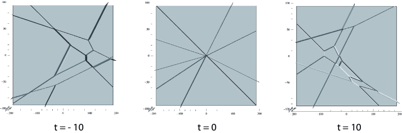
Figure 3. Example of contour plots $\operatorname{\mathcal{C}}_{t}(u_{A})$ for $A\in Gr_{4,9}$. The contour plots are obtained by “Plot3D” of Mathematica (see the details in the text).

Note that if there are two adjacent regions of the contour plot whose Plücker coordinates have different signs, then the line-soliton separating them is singular. For example, the line-soliton of type $[4,8]$ (the second soliton from the left in $y\gg 0$) is singular, because the Plücker coordinates corresponding to the (dominant exponentials of the) adjacent regions are

$$\Delta_{1,2,4,9}=p_{3}p_{5}p_{8}p_{10}p_{11}p_{12}p_{14}=1\qquad{\rm and}\qquad\Delta_{1,2,8,9}=-p_{8}p_{10}p_{11}p_{12}p_{14}=-1.$$

8. Unbounded line-solitons at $y\gg 0$ and $y\ll 0$

In this section we show that the unbounded line-solitons at $|y|\gg 0$ of a contour plot $\operatorname{\mathcal{C}}_{t}(u_{A})$ are determined by which positroid stratum contains $A$. Conversely, the unbounded line-solitons of $\operatorname{\mathcal{C}}_{t}(u_{A})$ determine which positroid stratum $A$ lies in. The main result of this section is Theorem 8.1.

Theorem 8.1.

Let $A\in Gr_{k,n}$ lie in the positroid stratum $S_{\pi^{:}}$, where $\pi^{:}=(\pi,col)$. Consider the contour plot $\operatorname{\mathcal{C}}_{t}(u_{A})$ for any time $t$. Then the excedances (respectively, nonexcedances) of $\pi$ are in bijection with the unbounded line-solitons of $\operatorname{\mathcal{C}}_{t}(u_{A})$ at $y\gg 0$ (respectively, $y\ll 0$). More specifically, in $\operatorname{\mathcal{C}}_{t}(u_{A})$,

• there is an unbounded line-soliton of $[i,h]$-type at $y\gg 0$ if and only if $\pi(i)=h$ for $i<h$,

• there is an unbounded line-soliton of $[i,h]$-type at $y\ll 0$ if and only if $\pi(h)=i$ for $i<h$.

Therefore $\pi^{:}$ determines the unbounded line-solitons at $y\gg 0$ and $y\ll 0$ of $\operatorname{\mathcal{C}}_{t}(u_{A})$ for any time $t$.

Conversely, given a contour plot $\operatorname{\mathcal{C}}_{t}(u_{A})$ at any time $t$ where $A\in Gr_{k,n}$, one can construct $\pi^{:}=(\pi,col)$ such that $A\in S_{\pi^{:}}$ as follows. The excedances and nonexcedances of $\pi$ are constructed as above from the unbounded line-solitons. If there is an $h\in[n]$ such that $h\in J$ for every dominant exponential $E_{J}$ labeling the contour plot, then set $\pi(h)=h$ with $col(h)=1$. If there is an $h\in[n]$ such that $h\notin J$ for any dominant exponential $E_{J}$ labeling the contour plot, then set $\pi(h)=h$ with $col(h)=-1$.

Proof. This result will follow immediately from Theorems 8.3 and 8.7 below.        

Remark 8.2.

Chakravarty and Kodama [5, Prop. 2.6 and 2.9] and [7, Theorem 5] associated a derangement to each irreducible element $A$ in the totally non-negative part $(Gr_{k,n})_{\geq 0}$ of the Grassmannian. Theorem 8.1 generalizes their result by dropping the hypothesis of irreducibility and extending the setting from $(Gr_{k,n})_{\geq 0}$ to $Gr_{k,n}$.

Before stating Theorems 8.3 and 8.7, we need to introduce some notation.

Given a matrix $A$ with $n$ columns, let $A(k,\dots,\ell)$ be the submatrix of $A$ obtained from columns $k,k+1,\dots,\ell-1,\ell$, where the columns are listed in the circular order $k,k+1,\dots,n-1,n,1,2,\dots,k-1$.

The following result generalizes [2, Lemma 3.4] from $(Gr_{k,n})_{\geq 0}$ to $Gr_{k,n}$. Our proof of Theorem 8.3 will be similar to that of [2], but some arguments can be clarified using some basic theory of matroids.

Theorem 8.3.

Let $A\in Gr_{k,n}$ and consider the contour plot $\operatorname{\mathcal{C}}_{t}(u_{A})$ for any time $t$. Choose $i,h\in\{1,\dots,n\}$ with $i<h$.

Then there is an unbounded line-soliton of $\operatorname{\mathcal{C}}_{t}(u_{A})$ at $y\ll 0$ labeled $[i,h]$ if and only if

(8.1) $$\mathop{\rm rank}\nolimits A(i,\dots,h-1)=\mathop{\rm rank}\nolimits A(i+1,\dots,h)=\mathop{\rm rank}\nolimits A(i,\dots,h)=\mathop{\rm rank}\nolimits A(i+1,\dots,h-1)+1.$$

There is an unbounded line-soliton of $\operatorname{\mathcal{C}}_{t}(u_{A})$ at $y\gg 0$ labeled $[i,h]$ if and only if

(8.2) $$\mathop{\rm rank}\nolimits A(h,\dots,i-1)=\mathop{\rm rank}\nolimits A(h+1,\dots,i)=\mathop{\rm rank}\nolimits A(h,\dots,i)=\mathop{\rm rank}\nolimits A(h+1,\dots,i-1)+1.$$

Recall from Section 6 that $\theta_{j}(x,y,z)=\kappa_{j}x+\kappa_{j}^{2}y+\kappa_{j}^{3}t$. Fix $i,j\in\{1,\dots,n\}$, and let $L_{i,j}$ denote the line defined by $\theta_{i}=\theta_{j}$. Define subsets of $[n]$ by

$$P =\{\max(i,j)+1,\dots,\min(i,j)-1\}:=\{1,\dots,\min(i,j)-1\}\cup\{\max(i,j)+1,\dots,n\}\text{ and }$$

$$Q =\{\min(i,j)+1,\dots,\max(i,j)-1\}.$$

In order to study the unbounded solitons at $y\gg 0$ and $y\ll 0$, we first record the following lemma.

Lemma 8.4.

[2, Lemma 3.1] For $|y|\gg 0$, we have the following ordering among the $\theta_{j}$’s on the line $L_{i,j}$:

1. For $y\gg 0$ on the line $L_{i,j}$, $\theta_{m}<\theta_{i}=\theta_{j}$ for all $m\in Q$, and $\theta_{m}>\theta_{i}=\theta_{j}$ for all $m\in P$.

2. For $y\ll 0$ on the line $L_{i,j}$, $\theta_{m}>\theta_{i}=\theta_{j}$ for all $m\in Q$, and $\theta_{m}<\theta_{i}=\theta_{j}$ for all $m\in P$.

Proof. For a fixed $t$, the equation of the line $L_{i,j}$ (which is defined by $\theta_{i}=\theta_{j}$) has the form

$$x+(\kappa_{i}+\kappa_{j})y={\rm constant}.$$

Then along $L_{i,j}$, we have

$$\theta_{m}-\theta_{m^{\prime}}=(\kappa_{m}-\kappa_{m^{\prime}})[(\kappa_{m}+\kappa_{m^{\prime}})-(\kappa_{i}+\kappa_{j})]y+\delta,$$

where $\delta$ does not depend on $x$ or $y$. The lemma now follows from the fact that $\kappa_{1}<\kappa_{2}<\cdots<\kappa_{n}$.        

Then it follows immediately that

Corollary 8.5.

For $y=y_{0}\gg 0$ (respectively $y=y_{0}\ll 0$) there is a well-defined total order on $\theta_{1},\dots,\theta_{n}$ on the line $L_{i,j}$ (with $\theta_{i}=\theta_{j}$), and this order does not change if we increase $y$ (resp., decrease $y$).

The following matroidal result will be useful to us.

Proposition 8.6.

[27, Theorem 1.8.5] Consider a matroid $\operatorname{\mathcal{M}}$ of rank $k$ on the set $[n]$, and let $\omega=(\omega_{1},\dots,\omega_{n})\in\mathbb{R}^{n}$. Define the weight of a basis $J=(j_{1},\dots,j_{k})$ of $\operatorname{\mathcal{M}}$ to be $\omega_{j_{1}}+\dots+\omega_{j_{k}}$. Then the basis (or bases) of maximal weight are precisely the possible outcomes of the greedy algorithm: Start with $J=\emptyset$. At each stage, look for an $\omega$-maximum element of $[n]$ which can be added to $J$ without making it dependent, and add it. After $k$ steps, output the basis $J$.

We now turn to the proof of Theorem 8.3. We will prove the result for unbounded line-solitons at $y\gg 0$ (the other part of the proof is analogous).

Proof. Let $\operatorname{\mathcal{M}}$ be the matroid associated to $A$. Its ground set $[n]$ is identified with the columns of $A$. First suppose that for $i,j\in[n]$, with $i>j$ we have

(8.3) $$\mathop{\rm rank}\nolimits A(i,\dots,j-1)=\mathop{\rm rank}\nolimits A(i+1,\dots,j)=\mathop{\rm rank}\nolimits A(i,\dots,j)=\mathop{\rm rank}\nolimits A(i+1,\dots,j-1)+1.$$

By Corollary 8.5, at $y\gg 0$ we have a well-defined total order on the $\theta_{m}$’s on the line $L_{i,j}$. At $y\gg 0$ the problem of computing the dominant exponential is equivalent to finding the basis of $\operatorname{\mathcal{M}}$ with the maximal weight with respect to $(\theta_{1},\dots,\theta_{n})$.

By Proposition 8.6, we can compute such a weight-maximal basis using the greedy algorithm. By Corollary 8.4, the greedy algorithm will first choose as many columns of $A(i+1,\dots,j-1)$ as possible. All of the $\theta_{m}$’s are distinct except for $\theta_{i}=\theta_{j}$, so there will be a unique way to add a maximal independent set of columns of $A(i+1,\dots,j-1)$ to the basis we are building. Note that by (8.3), the rank of $A(i+1,\dots,j-1)$ is less than $k$, so our weight-maximal basis must additionally contain at least one column that is not from $A(i+1,\dots,j-1)$. By Corollary 8.4, columns $i$ and $j$ share a weight which is greater than any of the other remaining columns, so the next step is to add one of columns $i$ and $j$ to the basis we are building. By (8.3), we cannot add both columns, because doing so will only increase the rank by $1$. Therefore we now have two ways to build a weight-maximal basis, by adding either one of the columns $i$ and $j$. If the two bases we are building do not yet have rank $k$, then there is now a unique way to add columns from $A(j+1,\dots,i-1)$ to complete both of them.

We have now shown that along $L_{i,j}$ at $y\gg 0$, there are precisely two dominant exponentials, $E_{I}$ and $E_{J}$, where $I=(J\cup\{i\})\setminus\{j\}$. Therefore there is an unbounded line-soliton at $y\gg 0$ labeled $[j,i]$.

Conversely, suppose that for $i>j$, there is an unbounded line-soliton labeled $[j,i]$ at $y\gg 0$. Then on the line $L_{i,j}$ there are two dominant exponentials $E_{I}$ and $E_{J}$ with $J=(I\cup\{j\})\setminus\{i\}$. By Proposition 8.6, these must be the two outcomes of the greedy algorithm. As before, by Corollary 8.4, the greedy algorithm will first choose as many columns of $A(i+1,\dots,j-1)$ as possible while keeping the collection linearly independent, and then the next step will be to add exactly one of the columns $i$ and $j$. Since neither dominant exponential contains both $i$ and $j$, adding both columns must not increase the rank more than adding just one of them. Therefore equation (8.3) must hold.        

Theorem 8.7.

Let $A\in Gr_{k,n}$ lie in the positroid stratum $S_{\pi^{:}}$ where $\pi^{:}=(\pi,col)$. Choose $1\leq i<h\leq n$. Then $\pi(h)=i$ if and only if equation (8.1) holds, and $\pi(i)=h$ if and only if equation (8.2) holds.

Proof. Let $\operatorname{\mathcal{I}}=(I_{1},\dots,I_{n})$ be the Grassmann necklace associated to $A$, so $\pi^{:}=\pi^{:}(\operatorname{\mathcal{I}}).$ Then by Lemma 2.10, $I_{i}=\{x_{1},x_{2},\dots,x_{k}\}$ is the lexicographically minimal $k$-subset with respect to the order $i<i+1<\dots<n<1<\dots<i-1$ such that $\Delta_{I_{i}}(A)\neq 0$. Similarly $I_{i+1}$ is the lexicographically minimal $k$-subset with respect to the order $i+1<\dots<n<1<\dots<i-1<i$ such that $\Delta_{I_{i+1}}(A)\neq 0$.

We will prove the first statement of the theorem (the proof of the second is analogous, so we omit it.) Suppose that $\pi(h)=i$. Then $x_{1}=i$; otherwise the $i$th column of $A$ is the zero-vector and $\pi(i)=i$. Using Definition 2.16 and Lemma 2.10, $h$ has the following characterization. Consider the column indices in the order $i+1,i+2,\dots,n,1,2,\dots,i$ and greedily choose the earliest index $h$ such that the columns of $A$ indexed by the set $\{x_{2},\dots,x_{k}\}\cup\{h\}$ are linearly independent. Then $I_{i+1}=(I_{i}\setminus\{i\})\cup\{h\}$.

Now consider the ranks of various submatrices of $A$ obtained by selecting certain columns.

Claim 0. $\mathop{\rm rank}\nolimits A(i+1,\dots,h-1,h)=1+\mathop{\rm rank}\nolimits A(i+1,\dots,h-1)$. This claim follows from the characterization of $h$ and the fact that $I_{i+1}$ is the lexicographically minimal $k$-subset with respect to the order $i+1<\dots<n<1<\dots<i$ such that $\Delta_{I_{i+1}}(A)\neq 0$.

Claim 1. $\mathop{\rm rank}\nolimits A(i,i+1,\dots,h)=\mathop{\rm rank}\nolimits A(i,i+1,\dots,h-1)$. To prove this claim, we consider two cases. Either $i<_{i}h<_{i}x_{k}$ or $i<_{i}x_{k}<_{i}h$, where $<_{i}$ is the total order $i<i+1<\dots<n<1<\dots<i-1$. In the first case, the claim follows, because $h$ is not contained in the set $I_{i}$. In the second case, $\mathop{\rm rank}\nolimits A(i,i+1,i+2,\dots,x_{k})=k$, and the index set $\{i,i+1,\dots,x_{k}\}$ is a proper subset of $\{i,i+1,\dots,h\}$, so $\mathop{\rm rank}\nolimits A(i,\dots,h)=\mathop{\rm rank}\nolimits A(i,\dots,h-1)=k$.

Now let $R=\mathop{\rm rank}\nolimits A(i+1,i+2,\dots,h-1)$. By Claim 0, $\mathop{\rm rank}\nolimits A(i+1,\dots,h)=R+1$. Therefore we have $\mathop{\rm rank}\nolimits A(i,\dots,h)\geq\mathop{\rm rank}\nolimits A(i+1,\dots,h)=R+1$. By Claim 1, $\mathop{\rm rank}\nolimits A(i,\dots,h)=\mathop{\rm rank}\nolimits A(i,\dots,h-1)$, but $\mathop{\rm rank}\nolimits A(i,\dots,h-1)\leq R+1$, so $\mathop{\rm rank}\nolimits A(i,\dots,h)\leq R+1$. We now have $\mathop{\rm rank}\nolimits A(i,\dots,h)=R+1$. But also $\mathop{\rm rank}\nolimits A(i,\dots,h-1)=\mathop{\rm rank}\nolimits A(i,\dots,h)=R+1$. Therefore $\mathop{\rm rank}\nolimits A(i,i+1,\dots,h-1)=\mathop{\rm rank}\nolimits A(i+1,\dots,h-1,h)=\mathop{\rm rank}\nolimits A(i,\dots,h)=\mathop{\rm rank}\nolimits A(i+1,\dots,h-1)+1$, as desired.

Conversely, suppose that $\mathop{\rm rank}\nolimits A(i,i+1,\dots,h-1)=\mathop{\rm rank}\nolimits A(i+1,\dots,h-1,h)=\mathop{\rm rank}\nolimits A(i,\dots,h)=\mathop{\rm rank}\nolimits A(i+1,\dots,h-1)+1$. Let $I_{i}$ and $I_{i+1}$ be the lexicographically minimal $k$-subsets with respect to the total orders $<_{i}$ and $<_{i+1}$, such that $\Delta_{I_{i}}(A)\neq 0$ and $\Delta_{I_{i+1}}(A)\neq 0$. Since $\mathop{\rm rank}\nolimits A(i,i+1,\dots,h-1)=\mathop{\rm rank}\nolimits A(i,\dots,h)$, we have $h\notin I_{i}$. And since $\mathop{\rm rank}\nolimits A(i+1,\dots,h-1,h)=\mathop{\rm rank}\nolimits A(i+1,\dots,h-1)+1$, we have $h\in I_{i+1}$. We now claim that $i\in I_{i}$. Otherwise, by the definition of Grassmann necklace, $I_{i+1}=I_{i}$, which contradicts the fact that $\mathop{\rm rank}\nolimits A(i,i+1,\dots,h-1)=\mathop{\rm rank}\nolimits A(i+1,\dots,h-1)+1$. Therefore the claim holds, and by Definition 2.16, we must have $\pi(h)=i$.        

9. Soliton graphs and generalized plabic graphs

The following notion of soliton graph forgets the metric data of the contour plot, but preserves the data of how line-solitons interact and which exponentials dominate.

Definition 9.1.

Let $A\in Gr_{k,n}$ and consider a generic contour plot $\operatorname{\mathcal{C}}_{t}(u_{A})$ for some time $t$. Color a trivalent vertex black (respectively, white) if it has a unique edge extending downwards (respectively, upwards) from it. We preserve the labeling of regions and edges that was used in the contour plot: we label a region by $E_{I}$ if the dominant exponential in that region is $\Delta_{I}E_{I}$, and label each line-soliton by its type $[i,j]$ (see Lemma 7.5). We also preserve the topology of the graph, but forget the metric structure. We call this labeled graph with bicolored vertices the soliton graph $G_{t_{0}}(u_{A})$.

Example 9.2.

We continue Example 7.9. Figure 4 contains the same contour plot $\operatorname{\mathcal{C}}_{t}(u_{A})$ as that at the left of Figure 3. One may use Lemma 7.5 to label all regions and edges in the soliton graph. After computing the Plücker coordinates, one can identify the singular solitons, which are indicated by the dotted lines in the soliton graph.

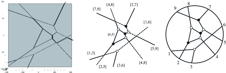
Figure 4. Example of a contour plot $\operatorname{\mathcal{C}}_{t}(u_{A})$, its soliton graph $C=G_{t}(u_{A})$, and its generalized plabic graph $Pl(C)$. The parameters used are those from Example 7.9. In particular, $(\kappa_{1},\dots,\kappa_{9})=(-5,-3,-2,-1,0,1,2,3,4)$, and $\pi=(6,7,1,8,2,3,9,4,5).$

We now describe how to pass from a soliton graph to a generalized plabic graph.

Definition 9.3.

A generalized plabic graph is an undirected graph $G$ drawn inside a disk with $n$ boundary vertices labeled $\{1,\dots,n\}$. We require that each boundary vertex $i$ is either isolated (in which case it is colored with color $1$ or $-1$), or is incident to a single edge; and each internal vertex is colored black or white. Edges are allowed to cross each other in an $X$-crossing (which is not considered to be a vertex).

By Theorem 8.1, the following construction is well-defined.

Definition 9.4.

Fix a positroid stratum ${\mathcal{S}}_{\pi^{:}}$ of $Gr_{k,n}$ where $\pi^{:}=(\pi,col)$. To each soliton graph $C$ coming from a point of that stratum we associate a generalized plabic graph $Pl(C)$ by:

• embedding $C$ into a disk, so that each unbounded line-soliton of $C$ ends at a boundary vertex;

• labeling the boundary vertex incident to the edge with labels $i$ and $\pi(i)$ by $\pi(i)$;

• adding an isolated boundary vertex labeled $h$ with color $1$ (respectively, $-1$) whenever $h\in J$ for each region label $E_{J}$ (respectively, whenever $h\notin J$ for any region label $E_{J}$);

• forgetting the labels of all edges and regions.

See Figure 4 for a soliton graph $C$ together with the corresponding generalized plabic graph $Pl(C)$.

Definition 9.5.

Given a generalized plabic graph $G$, the trip $T_{i}$ is the directed path which starts at the boundary vertex $i$, and follows the “rules of the road”: it turns right at a black vertex, left at a white vertex, and goes straight through the $X$-crossings. Note that $T_{i}$ will also end at a boundary vertex. If $i$ is an isolated vertex, then $T_{i}$ starts and ends at $i$. Define $\pi_{G}(i)=j$ whenever $T_{i}$ ends at $j$. It is not hard to show that $\pi_{G}$ is a permutation, which we call the trip permutation.

We use the trips to label the edges and regions of each generalized plabic graph.

Definition 9.6.

Given a generalized plabic graph $G$, start at each non-isolated boundary vertex $i$ and label every edge along trip $T_{i}$ with $i$. Such a trip divides the disk containing $G$ into two parts: the part to the left of $T_{i}$, and the part to the right. Place an $i$ in every region which is to the left of $T_{i}$. If $h$ is an isolated boundary vertex with color $1$, put an $h$ in every region of $G$. After repeating this procedure for each boundary vertex, each edge will be labeled by up to two numbers (between $1$ and $n$), and each region will be labeled by a collection of numbers. Two regions separated by an edge labeled by both $i$ and $j$ will have region labels $S$ and $(S\setminus\{i\})\cup\{j\}$. When an edge is labeled by two numbers $i<j$, we write $[i,j]$ on that edge, or $\{i,j\}$ or $\{j,i\}$ if we do not wish to specify the order of $i$ and $j$.

Although the following result was proved for irreducible cells of $(Gr_{k,n})_{\geq 0}$, the same proof holds for arbitrary positroid strata of $Gr_{k,n}$.

Theorem 9.7.

[21, Theorem 7.6] Consider a soliton graph $C=G_{t}(u_{A})$ coming from a point $A$ of a positroid stratum ${\mathcal{S}}_{\pi^{:}}$, where $\pi^{:}=(\pi,col)$. Then the trip permutation of $Pl(C)$ is $\pi$, and by labeling edges of $Pl(C)$ according to Definition 9.6, we will recover the original edge and region labels in $C$.

We invite the reader to verify Theorem 9.7 for the graphs in Figure 4.

Remark 9.8.

By Theorem 9.7, we can identify each soliton graph $C$ with its generalized plabic graph $Pl(C)$. From now on, we will often ignore the labels of edges and regions of a soliton graph, and simply record the labels on boundary vertices.

10. The contour plot for $t\ll 0$

Consider a matroid stratum $S_{\mathcal{M}}$ contained in the Deodhar component $S_{{D}}$, where $D$ is the corresponding or Go-diagram. From Definition 7.1 it is clear that the contour plot associated to any $A\in S_{\mathcal{M}}$ depends only on $\mathcal{M}$, not on $A$. In fact for $t\ll 0$ a stronger statement is true – the contour plot for any $A\in S_{\mathcal{M}}\subset S_{D}$ depends only on $D$, and not on $\mathcal{M}$. In this section we will explain how to use $D$ to construct first a generalized plabic graph $G_{-}(D)$, and then the contour plot $\operatorname{\mathcal{C}}_{t}(\mathcal{M})$ for $t\ll 0.$

10.1. Definition of the contour plot for $t\ll 0$.

Recall from (7.1) the definition of $f_{\mathcal{M}}(x,y,t)$. To understand how it behaves for $t\ll 0$, let us rescale everything by $t$. Define $\bar{x}=\frac{x}{t}$ and $\bar{y}=\frac{y}{t}$, and set

$$\phi_{i}(\bar{x},\bar{y})=\kappa_{i}\bar{x}+\kappa_{i}^{2}\bar{y}+\kappa_{i}^{3},$$

that is, $\kappa_{i}x+\kappa_{i}^{2}y+\kappa_{i}^{3}t=t\phi_{i}(\bar{x},\bar{y})$. Note that because $t$ is negative, $x$ and $y$ have the opposite signs of $\bar{x}$ and $\bar{y}$. This leads to the following definition of the contour plot for $t\ll 0$.

Definition 10.1.

We define the contour plot $\operatorname{\mathcal{C}}_{-\infty}(\mathcal{M})$ to be the locus in $\mathbb{R}^{2}$ where

$$\underset{J\in\mathcal{M}}{\min}\left\{\mathop{\textstyle\sum}\limits_{i=1}^{k}\phi_{j_{i}}(\bar{x},\bar{y})\right\}\quad\text{ is not linear .}$$

Remark 10.2.

After a $180^{\circ}$ rotation, $\operatorname{\mathcal{C}}_{-\infty}(\mathcal{M})$ is the limit of $\operatorname{\mathcal{C}}_{t}(u_{A})$ as $t\to-\infty$, for any $A\in S_{\mathcal{M}}$. Note that the rotation is required because the positive $x$-axis (respectively, $y$-axis) corresponds to the negative $\bar{x}$-axis (respectively, $\bar{y}$-axis).

Definition 10.3.

Define $v_{i,\ell,m}$ to be the point in $\mathbb{R}^{2}$ where $\phi_{i}(\bar{x},\bar{y})=\phi_{\ell}(\bar{x},\bar{y})=\phi_{m}(\bar{x},\bar{y}).$ A simple calculation yields that the point $v_{i,\ell,m}$ has the following coordinates in the $\bar{x}\bar{y}$-plane:

$$v_{i,\ell,m}=(\kappa_{i}\kappa_{\ell}+\kappa_{i}\kappa_{m}+\kappa_{\ell}\kappa_{m},-(\kappa_{i}+\kappa_{\ell}+\kappa_{m})).$$

Some of the points $v_{i,\ell,m}\in\mathbb{R}^{2}$ correspond to trivalent vertices in the contour plots we construct; such a point is the location of the resonant interaction of three line-solitons of types $[i,\ell]$, $[\ell,m]$ and $[i,m]$ (see Theorem 10.6 below). Because of our assumption on the genericity of the $\kappa$-parameters, those points are all distinct.

10.2. Main results on the contour plot for $t\ll 0$

The results of this section generalize those of [20, Section 8] to a soliton solution coming from an arbitrary point of the real Grassmannian (not just the non-negative part). We start by giving an algorithm to construct a generalized plabic graph $G_{-}(D)$, which will be used to construct $\operatorname{\mathcal{C}}_{-\infty}(\mathcal{M})$. Figure 5 illustrates the steps of Algorithm 10.4, starting from the Go-diagram of the Deodhar component $S_{D}$ where $D$ is as in the upper left corner of Figure 5.

Algorithm 10.4.

From a Go-diagram $D$ to $G_{-}(D)$:

1. Start with a Go-diagram $D$ contained in a $k\times(n-k)$ rectangle, and replace each  ,  , and blank box by a cross, a cross, and a pair of elbows, respectively. Label the $n$ edges along the southeast border of the Young diagram by the numbers $1$ to $n$, from northeast to southwest. The configuration of crosses and elbows forms $n$ “pipes” which travel from the southeast border to the northwest border; label the endpoint of each pipe by the label of its starting point.

2. Add a pair of black and white vertices to each pair of elbows, and connect them by an edge, as shown in the upper right of Figure 5. Forget the labels of the southeast border. If there is an endpoint of a pipe on the east or south border whose pipe starts by going straight, then erase the straight portion preceding the first elbow. If there is a horizontal (respectively, vertical) pipe starting at $i$ with no elbows, then erase it, and add an isolated boundary vertex labeled $i$ with color $1$ (respectively, $-1$).

3. Forget any degree $2$ vertices, and forget any edges of the graph which end at the southeast border of the diagram. Denote the resulting graph $G_{-}(D)$.

4. After embedding the graph in a disk with $n$ boundary vertices (including isolated vertices) we obtain a generalized plabic graph, which we also denote $G_{-}(D)$. If desired, stretch and rotate $G_{-}(D)$ so that the boundary vertices at the west side of the diagram are at the north instead.

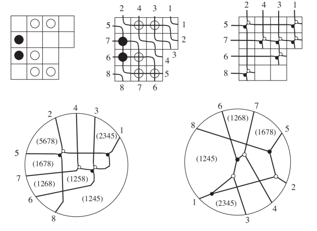
Figure 5. Construction of the generalized plabic graph $G_{-}(D)$ associated to the Go-diagram $D$. The labels of the regions of the graph indicate the index sets of the corresponding Plücker coordinates. Using the notation of Definition 4.10, we have $\pi(D)=vw^{-1}=(5,7,1,6,8,3,4,2)$.

Remark 10.5.

If there are no black stones in $D$, then this algorithm reduces to [21, Algorithm 8.7]. In this case, by [21, Theorem 11.15], the Plücker coordinates corresponding to the regions of $G_{-}(D)$ include the set of minors ${\mathcal{J}}$ described in Theorem 5.13. In particular, the set of Plücker coordinates labeling the regions of $G_{-}(D)$ comprise a positivity test for $S_{D}$.

The following is the main result of this section.

Theorem 10.6.

Choose a matroid stratum $S_{\mathcal{M}}$ and let $S_{D}$ be the Deodhar component containing $S_{\mathcal{M}}$. Recall the definition of $\pi(D)$ from Definition 4.10. Use Algorithm 10.4 to obtain $G_{-}(D)$. Then $G_{-}(D)$ has trip permutation $\pi(D)$, and we can use it to explicitly construct $\operatorname{\mathcal{C}}_{-\infty}(\operatorname{\mathcal{M}})$ as follows. Label the edges of $G_{-}(D)$ according to the rules of the road. Label by $v_{i,\ell,m}$ each trivalent vertex which is incident to edges labeled $[i,\ell]$, $[i,m]$, and $[\ell,m]$, and give that vertex the coordinates $(\bar{x},\bar{y})=(\kappa_{i}\kappa_{\ell}+\kappa_{i}\kappa_{m}+\kappa_{\ell}\kappa_{m},-(\kappa_{i}+\kappa_{\ell}+\kappa_{m}))$. Replace each edge labeled $[i,j]$ which ends at a boundary vertex by an unbounded line-soliton with slope $\kappa_{i}+\kappa_{j}$. (Each edge labeled $[i,j]$ between two trivalent vertices will automatically have slope $\kappa_{i}+\kappa_{j}$.) In particular, $\operatorname{\mathcal{C}}_{-\infty}(\operatorname{\mathcal{M}})$ is determined by $D$. Recall from Remark 10.2 that after a $180^{\circ}$ rotation, $\operatorname{\mathcal{C}}_{-\infty}(\operatorname{\mathcal{M}})$ is the limit of $\operatorname{\mathcal{C}}_{t}(u_{A})$ as $t\to-\infty$, for any $A\in S_{\mathcal{M}}$.

Remark 10.7.

Since the contour plot $\operatorname{\mathcal{C}}_{-\infty}(\operatorname{\mathcal{M}})$ depends only on $D$, we also refer to it as $\operatorname{\mathcal{C}}_{-\infty}(D)$.

Remark 10.8.

The results of this section may be extended to the case $t\gg 0$ by duality considerations (similar to the way in which our previous paper [21] described contour plots for both $t\ll 0$ and $t\gg 0$). Note that the Deodhar decomposition of $Gr_{k,n}$ depends on a choice of ordered basis $(e_{1},\dots,e_{n})$. Using the ordered basis $(e_{n},\dots,e_{1})$ instead and the corresponding Deodhar decomposition, one may explicitly describe contour plots at $t\gg 0$.

Remark 10.9.

Depending on the choice of the parameters $\kappa_{i}$, the contour plot $\operatorname{\mathcal{C}}_{-\infty}(D)$ may have a slightly different topological structure than the soliton graph $G_{-}(D)$. While the incidences of line-solitons with trivalent vertices are determined by $G_{-}(D)$, the locations of $X$-crossings may vary based on the $\kappa_{i}$’s. More specifically, changing the $\kappa_{i}$’s may change the contour plot via a sequence of slides, see Section 11.

Our proof of Theorem 10.6 is similar to the proof of [20, Theorem 8.9]. The main strategy is to use induction on the number of rows in the Go-diagram $D$. More specifically, let $D^{\prime}$ denote the Go-diagram $D$ with its top row removed. In Lemma 10.11 we will explain that $G_{-}(D^{\prime})$ can be seen as a labeled subgraph of $G_{-}(D)$. In Theorem 10.14, we will explain that there is a polyhedral subset of $\operatorname{\mathcal{C}}_{-\infty}(D)$ which coincides with $\operatorname{\mathcal{C}}_{-\infty}({D^{\prime}})$. And moreover, every vertex of $\operatorname{\mathcal{C}}_{-\infty}({D^{\prime}})$ appears as a vertex of $\operatorname{\mathcal{C}}_{-\infty}({D})$. By induction we can assume that Theorem 10.6 correctly computes $\operatorname{\mathcal{C}}_{-\infty}(D^{\prime})$, which in turn provides us with a description of “most” of $\operatorname{\mathcal{C}}_{-\infty}(D)$, including all line-solitons and vertices whose indices do not include $1$. On the other hand, Theorem 8.1 gives a complete description of the unbounded solitons of both $\operatorname{\mathcal{C}}_{-\infty}({D^{\prime}})$ and $\operatorname{\mathcal{C}}_{-\infty}({D})$ in terms of $\pi(D^{\prime})$ and $\pi(D)$. In particular, $\operatorname{\mathcal{C}}_{-\infty}({D})$ contains one more unbounded soliton at $y\gg 0$ than does $\operatorname{\mathcal{C}}_{-\infty}({D})$. This information together with the resonance property allows us to complete the description of $\operatorname{\mathcal{C}}_{-\infty}({D})$ and match it up with the combinatorics of $G_{-}(D)$.

Lemma 10.10.

The generalized plabic graph $G_{-}(D)$ from Algorithm 10.4 has trip permutation $\pi(D)$.

Proof. If we follow the rules of the road starting from a boundary vertex of $G_{-}(D)$, we will first follow a “pipe” southeast (compare the lower left and the top middle pictures in Figure 5) and then travel straight west along the row or north along the column where that pipe ended. Recall from Definition 4.10 that $\pi(D)=vw^{-1}$. Noting that we can read off $v$ and $w$ from the pipes in the top middle picture of Figure 5, we see that following the rules of the road has the same effect as computing $vw^{-1}$.        

The next lemma explains the relationship between $G_{-}(D)$ and $G_{-}(D^{\prime})$, where $D^{\prime}$ is the Go-diagram $D$ with the top row removed. It should be clear after examining Figure 6.

Figure 6. Inductive construction of the generalized plabic graph $G_{-}(D)$ associated to the Go-diagram $D$, cf. Figure 5.

Lemma 10.11.

Let $D$ be a Go-diagram with $k$ rows and $n-k$ columns, and let $G=G_{-}(D)$ be the edge-labeled plabic graph constructed by Algorithm 10.4. Form a new Go-diagram $D^{\prime}$ from $D$ by removing the top row of $D$; suppose that $\ell$ is the sum of the number of rows and columns in $D^{\prime}$. Let $G^{\prime}$ be the edge-labeled plabic graph associated to $D^{\prime}$, but instead of using the labels $\{1,2,\dots,\ell\}$, use the labels $\{n-\ell+1,n-\ell+2,\dots,n\}$. Let $h$ denote the label of the top row of $D$. Then $G^{\prime}$ is obtained from $G$ by removing the trip $T_{h}$ starting at $h$ and all edges to its right which have a trivalent vertex on $T_{h}$.

From now on, we will assume without loss of generality that $i_{1}=1$ is a pivot for $A\in S_{D}$.

Definition 10.12.

Let $\mathcal{M}$ be a matroid on $[n]$ such that $1$ is contained in at least one base. Let $\mathcal{M^{\prime}}$ be the matroid $\{J\setminus\{1\}\ |\ 1\in J\text{ and }J\in\mathcal{M}\}.$

Using arguments similar to those in the proof of Theorem 5.6, one can verify the following.

Lemma 10.13.

If $A\in S_{\operatorname{\mathcal{M}}}\subset S_{D}$ is in row-echelon form and $A^{\prime}$ is the span of rows $2,3,\dots,k$ in $A\in S_{\mathcal{M}}\subset Gr_{k,n}$, then $A^{\prime}\in S_{\mathcal{M^{\prime}}}\subset S_{D^{\prime}}$, where $D^{\prime}$ is obtained from $D$ by removing its top row.

The following result is a combination of [20, Theorem 8.17] and [20, Corollary 8.18]. Although in [20] the context was $A\in(Gr_{k,n})_{\geq 0}$ and in this paper we are allowing $A\in Gr_{k,n}$, the proofs from [20] hold without any modification. See Figure 7 for an illustration of the theorem.

Theorem 10.14.

[20] Let $\mathcal{M}$ be a matroid such that $1$ is contained in at least one base. Then there is an unbounded polyhedral subset $\mathcal{R}$ of $\operatorname{\mathcal{C}}_{-\infty}({\mathcal{M}})$ whose boundary is formed by line-solitons, such that every region in $\mathcal{R}$ is labeled by a dominant exponential $E_{J}$ such that $1\in J$. In $\mathcal{R}$, $\operatorname{\mathcal{C}}_{-\infty}(\mathcal{M})$ coincides with $\operatorname{\mathcal{C}}_{-\infty}(\mathcal{M^{\prime}})$. Moreover, every region of $\operatorname{\mathcal{C}}_{-\infty}(\mathcal{M^{\prime}})$ which is incident to a trivalent vertex and labeled by $E_{J^{\prime}}$ corresponds to a region of $\operatorname{\mathcal{C}}_{-\infty}(\mathcal{M})$ which is labeled by $E_{J^{\prime}\cup\{1\}}$.

In particular, the set of trivalent vertices in $\operatorname{\mathcal{C}}_{-\infty}(\mathcal{M})$ is equal to the set of trivalent vertices in $\operatorname{\mathcal{C}}_{-\infty}(\mathcal{M^{\prime}})$ together with some vertices of the form $v_{1,b,c}$. These vertices comprise the vertices along the trip $T_{1}$ (the set of line-solitons labeled $[1,j]$ for any $j$). In particular, every line-soliton in $\operatorname{\mathcal{C}}_{-\infty}(\mathcal{M})$ which was not present in $\operatorname{\mathcal{C}}_{-\infty}(\mathcal{M^{\prime}})$ and is not on $T_{1}$ must be unbounded. And every new bounded line-soliton in $\operatorname{\mathcal{C}}_{-\infty}(\mathcal{M})$ that did not come from a line-soliton in $\operatorname{\mathcal{C}}_{-\infty}(\mathcal{M^{\prime}})$ is of type $[1,j]$ for some $j$.

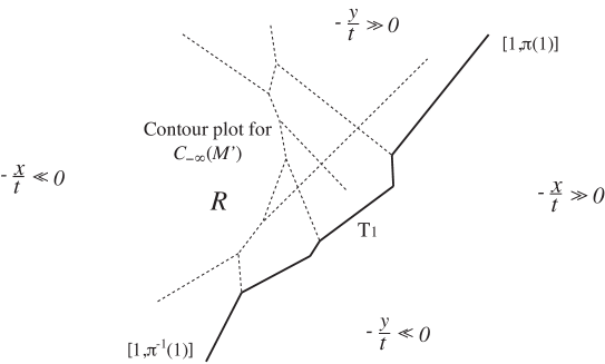
Figure 7. The contour plot $\operatorname{\mathcal{C}}_{-\infty}(\mathcal{M^{\prime}})$ within the contour plot $\operatorname{\mathcal{C}}_{-\infty}(\mathcal{M}).$

We now prove Theorem 10.6, using the characterization of unbounded line-solitons in Theorem 8.1.

Proof. Choose $A$ in the Deodhar component $S_{D}$. Let $\operatorname{\mathcal{M}}$ be the matroid such that $A\in S_{\operatorname{\mathcal{M}}}$. We will prove Theorem 10.6 using induction on the number of rows of $A$. Using the notation of Definition 10.12 and Lemma 10.13, we have that $A^{\prime}\in S_{\operatorname{\mathcal{M}}^{\prime}}\subset S_{D^{\prime}}$.

By Theorem 10.14, the contour plot $\operatorname{\mathcal{C}}_{-\infty}(\mathcal{M})$ is equal to the contour plot $\operatorname{\mathcal{C}}_{-\infty}(\mathcal{M^{\prime}})$ together with some trivalent vertices of the form $v_{1,b,c}$, all edges along the trip $T_{1}$, and some new unbounded line-solitons (which are all to the right of the trip $T_{1}$). By the inductive hypothesis, $\operatorname{\mathcal{C}}_{-\infty}(\mathcal{M^{\prime}})$ is constructed by Theorem 10.6; in particular, Algorithm 10.4 produces a (generalized) plabic graph which describes the trivalent vertices of $\operatorname{\mathcal{C}}_{-\infty}(\mathcal{M^{\prime}})$ and the interactions of all line-solitons at trivalent vertices.

Using Lemma 10.10 and Theorem 8.1, we see that Algorithm 10.4 produces a (generalized) plabic graph whose labels on unbounded edges agree with the labels of the unbounded line-solitons for the contour plot $\operatorname{\mathcal{C}}_{-\infty}(\mathcal{M})$ of any $A\in S_{D}$. The same is true for $A^{\prime}\in S_{D^{\prime}}$.

By Lemma 10.11, the plabic graph $G$ which Algorithm 10.4 associates to $D$ is equal to $G^{\prime}$ together with the trip $T_{1}$ starting at $1$ at some new line-solitons emanating right from trivalent vertices of $T_{1}$.

We now characterize the new vertices and line-solitons which $\operatorname{\mathcal{C}}_{-\infty}(\mathcal{M})$ contains, but which $\operatorname{\mathcal{C}}_{-\infty}(\mathcal{M^{\prime}})$ did not. We claim that the set of new vertices is precisely the set of $v_{1,b,c}$ (where $1<b<c$), such that either $c\to b$ is a nonexcedance of $\pi=\pi(\mathcal{M})$, or $c\to b$ is a nonexcedance of $\pi^{\prime}=\pi(\mathcal{M^{\prime}})$, but not both. Moreover, if $c\to b$ is a nonexcedance of $\pi$, then $v_{1,b,c}$ is white, while if $c\to b$ is a nonexcedance of $\pi^{\prime}$, then $v_{1,b,c}$ is black. The proof is identical to that of the same claim in the proof of [21, Theorem 8.8].

Now, if one analyzes the steps of Algorithm 10.4 (see in particular the second and third diagrams in Figure 5), it becomes apparent that the above description also characterizes the set of new vertices which the algorithm associates to the top row of the Go-diagram $D$. In particular, the nonexcedances of the corresponding permutation $\pi$ correspond to the vertical edges at the top of the second and third diagrams; when one labels these edges using the rules of the road, each edge gets the label $[b,c]$, where $b$ comes from the label of its pipe, and $c$ comes from the label of its column (shown at the bottom of the second diagram). The nonexcedances of $\pi^{\prime}$ are labeled in the same way but come from vertical edges which are present in the second row of $D$. Therefore each new trivalent vertex in the top row gets the label $v_{1,b,c}$ where $b$ and $c$ are as above, and where $c\to b$ is a nonexcedance of precisely one of $\pi$ and $\pi^{\prime}$.

Finally, we discuss the order in which the vertices $v_{1,b,c}$ occur along the trip $T_{1}$ in the contour plot. First note that the trip $T_{1}$ starts at $y\ll 0$ and along each line-soliton it always heads up (towards $y\gg 0$). This follows from the resonance condition (see e.g. [21, Figure 9] and take $i=1$). Therefore the order in which we encounter the vertices $v_{1,b,c}$ along the trip is given by the total order on the $y$-coordinates of the vertices, namely $\kappa_{1}+\kappa_{b}+\kappa_{c}$.

We now claim that this total order is identical to the total order on the positive integers $1+b+c$ – that is, it does not depend on the choice of $\kappa_{i}$’s, as long as $\kappa_{1}<\dots<\kappa_{n}$. If we can show this, then we will be done, because this is precisely the order in which the new vertices occur along the trip $T_{1}$ in the graph $G_{-}(L)$.

To prove the claim, it is enough to show that among the set of new vertices $v_{1,b,c}$, there are not two of the form $v_{1,i,\ell}$ and $v_{1,j,k}$ where $i<j<k<\ell$. To see this, recall that the indices $b$ and $c$ of the new vertices $v_{1,b,c}$ can be read off from the second and third diagrams illustrating Algorithm 10.4: $c$ will come from the bottom label of the corresponding column, while $b$ will come from the label of the pipe that $v_{1,b,c}$ lies on. Therefore, if there are two new vertices $v_{1,i,\ell}$ and $v_{1,j,k}$, then they must come from a pair of pipes which have crossed each other an odd number of times, as in Figure 8.

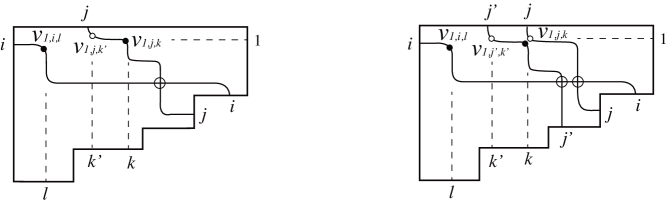
Figure 8.

Note that the second diagram of Figure 5 depicts a “pipe dream” (or “wiring diagram”) encoding the distinguished subexpression $\mathbf{v}$ of a reduced expression $\mathbf{w}$. If two pipes pass over each other in a given box we will say that they cross at that box, while if two pipes pass through the same box without crossing, we will say that they kiss at that box. Let us now follow a pair of pipes from southeast to northwest. The property of $\mathbf{v}$ being distinguished mean that two pipes starting at $i$ and $j$ must not kiss each other after having crossed each other an odd number of times.

Assume that Algorithm 10.4 produces two vertices $v_{1,i,\ell}$ and $v_{1,j,k}$ where $i<j<k<\ell$. Choose such a pair of vertices which minimizes $|\ell-k|$. We consider two cases, based on whether $v_{1,j,k}$ is black or white. In the first case (see the left of Figure 8), since $v_{1,j,k}$ is black, its pipe $j$ will continue west from $v_{1,j,k}$ and must eventually turn up, at some column $k^{\prime}$ such that $k<k^{\prime}<\ell$. But then Algorithm 10.4 produces another vertex $v_{1,j,k^{\prime}}$ such that $i<j<k^{\prime}<\ell$, so this vertex together with $v_{1,i,\ell}$ form a pair of vertices where $|\ell-k^{\prime}|<|\ell-k|$, contradicting our assumption of minimality of $|\ell-k|$.

In the second case (see the right of Figure 8), since $v_{1,j,k}$ is white, there is another black vertex $v_{1,j^{\prime},k}$ to its left in the same box $b$, whose pipe starts at $j^{\prime}$. Because $\mathbf{v}$ is distinguished, $j^{\prime}$ must be greater than $j$. (Otherwise the pipes starting at $j$ and $j^{\prime}$ would cross each other an odd number of times and then kiss at box $b$.) Now since $v_{1,j^{\prime},k}$ is black, its pipe must travel west from it and eventually turn up, at some column $k^{\prime}$ such that $j^{\prime}<k^{\prime}<\ell$. But then Algorithm 10.4 produces another vertex $v_{1,j^{\prime},k^{\prime}}$ such that $i<j^{\prime}<k^{\prime}<\ell$. But now we have a pair of vertices $v_{1,i,\ell}$ and $v_{1,j^{\prime},k^{\prime}}$ such that $i<j^{\prime}<k^{\prime}<\ell$ where $|\ell-k^{\prime}|<|\ell-k|$. This contradicts our assumption of minimality of $|\ell-k|$, and completes the proof of the claim.

Finally, using Definition 10.3 for the vertex $v_{i,\ell,m}$, we obtain the contour plot from $G$ by giving the trivalent vertices the explicit coordinates from Theorem 10.6.        

11. $X$-crossings, slides, and contour plots

In this section we discuss how our choice of the parameters $\kappa_{i}$ may affect the topology of the contour plot $\operatorname{\mathcal{C}}_{-\infty}(D)$ (and hence $\operatorname{\mathcal{C}}_{t}(u_{A})$ for $t\ll 0$ and $A\in S_{D}$), namely, by changing the locations of the $X$-crossings. See Remark 10.9. We also discuss the relation between $X$-crossings and Plücker coordinates.

11.1. Slides and the topology of contour plots

The following definition will be useful for understanding the dependence of the contour plot on the $\kappa_{i}$’s.

Figure 9. Some slides involving white $X$-crossings. These contour plots correspond to the same Le-diagram $D$ with $\pi(D)=(5,3,2,1,4)$, but they differ from $G_{-}(D)$.

Definition 11.1.

Consider a generalized plabic graph $G$ with at least one $X$-crossing. Let $v_{a,b,c}$ be a trivalent vertex (with edges labeled $[a,b]$, $[a,c]$, and $[b,c]$) which has a small neighborhood $N$ containing one or two $X$-crossings with a line labeled $[i,j]$, but no other trivalent vertices or $X$-crossings. Here $\{a,b,c\}$ and $\{i,j\}$ must be disjoint. Then a slide is a local deformation of the graph $G$ which moves the line $[i,j]$ so that it intersects a different set of edges of $v_{a,b,c}$, creating or destroying at most one region in the process.

See Figure 9 for examples. Recall the notions of black and white $X$-crossings from Definition 7.7.

Remark 11.2.

Theorem 10.6 determines everything about the combinatorics and topology of the contour plot $\operatorname{\mathcal{C}}_{-\infty}(D)$ except for which pairs of line-solitons form an $X$-crossing. Therefore if one deforms the parameters $\kappa_{i}$, the only way that the contour plot can change so as to change the topology is via a sequence of slides.

See Figure 10 for an example of two different contour plots associated to the same Go-diagram and element $A\in Gr_{4,8}$, but obtained using different choices of the $\kappa$-parameters. The two contour plots differ by precisely one slide. For another example, compare Figure 4 to Figure 11. Both of them are based on the Go-diagram from Example 7.9 and the same matrix $A$. The only difference is the value of $\kappa_{1}$. Note that this affects the $X$-crossings formed by the unbounded $[1,6]$ line-soliton, and that one contour plot can be obtained from the other via a sequence of three slides.

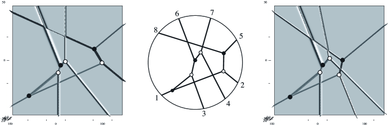
Figure 10. Contour plots $\operatorname{\mathcal{C}}_{t}(u_{A})$ constructed using the same $t$ and $A\in S_{D}\subset Gr_{4,8}$ but with different choices of the $\kappa$-parameters. The left plot uses $(\kappa_{1},\ldots,\kappa_{8})=(-3.5,-2,-1,0,0.5,1,2,5)$ while the right one uses $(-3.5,-2,-1,0,0.5,1,2.5,3)$. This affects the location of the $[4,7]$ line-soliton. In the middle we have the generalized plabic graph $G_{-}(D)$ using the Go-diagram $D$ of Figure 5.

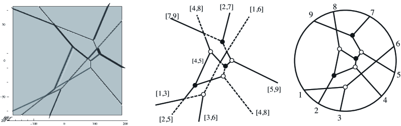
Figure 11. A contour plot $\operatorname{\mathcal{C}}_{t}(u_{A})$, soliton graph $C=G_{t}(u_{A})$ and generalized plabic graph $G_{-}(D)$ coming from a Go-diagram where $A\in S_{D}$. The $\kappa$-parameters are the same as those used for Figure 4 except that $\kappa_{1}=-3.1$ now, i.e. $(\kappa_{1},\ldots,\kappa_{9})=(-3.1,-3,-2,-1,0,1,2,3,4)$.

We now show that a slide on a contour plot preserves the number of black $X$-crossings.

Theorem 11.3.

Consider two contour plots $\operatorname{\mathcal{C}}$ and $\operatorname{\mathcal{C}}^{\prime}$ (for the same $A\in Gr_{k,n}$ and time $t$ but for different $\kappa$-parameters) which differ by a slide. Then $\operatorname{\mathcal{C}}$ and $\operatorname{\mathcal{C}}^{\prime}$ have the same number of black $X$-crossings.

Proof. Suppose that $\operatorname{\mathcal{C}}$ and $\operatorname{\mathcal{C}}^{\prime}$ differ by a slide involving the trivalent vertex $v_{a,b,c}$ and the line-soliton $[i,j]$ for $a<b<c$ and $i<j$, where the sets $\{a,b,c\}$ and $\{i,j\}$ are disjoint. We assume that $v_{a,b,c}$ is white. (The case where it is black is analogous.) There are five cases to consider:

1. $i<a<j<b<c$, which implies that $\kappa_{i}+\kappa_{j}<\kappa_{a}+\kappa_{b}<\kappa_{a}+\kappa_{c}<\kappa_{b}+\kappa_{c}.$

2. $i<a<b<j<c$, which implies that (a.) $\kappa_{i}+\kappa_{j}<\kappa_{a}+\kappa_{b}<\kappa_{a}+\kappa_{c}<\kappa_{b}+\kappa_{c}$, or
   (b.) $\kappa_{a}+\kappa_{b}<\kappa_{i}+\kappa_{j}<\kappa_{a}+\kappa_{c}<\kappa_{b}+\kappa_{c}$.

3. $a<i<b<j<c$, which implies that (a.) $\kappa_{a}+\kappa_{b}<\kappa_{i}+\kappa_{j}<\kappa_{a}+\kappa_{c}<\kappa_{b}+\kappa_{c}$, or
   (b.) $\kappa_{a}+\kappa_{b}<\kappa_{a}+\kappa_{c}<\kappa_{i}+\kappa_{j}<\kappa_{b}+\kappa_{c}$.

4. $a<i<b<c<j$, which implies that (a.) $\kappa_{a}+\kappa_{b}<\kappa_{a}+\kappa_{c}<\kappa_{i}+\kappa_{j}<\kappa_{b}+\kappa_{c}$, or
   (b.) $\kappa_{a}+\kappa_{b}<\kappa_{a}+\kappa_{c}<\kappa_{b}+\kappa_{c}<\kappa_{i}+\kappa_{j}$.

5. $a<b<i<c<j$, which implies that $\kappa_{a}+\kappa_{b}<\kappa_{a}+\kappa_{c}<\kappa_{b}+\kappa_{c}<\kappa_{i}+\kappa_{j}.$

(Note that any other ordering on $a,b,c,i,j$, such as $i<j<a<b<c$, would imply that there are no black $X$-crossings involving the edges incident to $v_{a,b,c}$ and the $[i,j]$ soliton.)

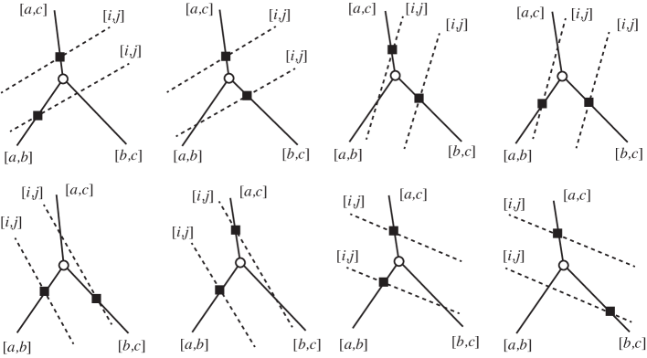
Figure 12. Various types of $X$-crossings involving the line-solitons incident to $v_{a,b,c}$ and the $[i,j]$ line-soliton. The top row shows Cases 1, 2a, 2b, and 3a from left to right, while the bottom row shows Cases 3b, 4a, 4b, and 5 from left to right.

Consider Case 1. Recall that “slope” of the $[i,j]$ line-soliton – that is, the tangent of the angle measured counterclockwise from the positive $y$-axis to the $[i,j]$ line-soliton – is equal to $\kappa_{i}+\kappa_{j}$. Therefore from the order on the slopes, the $[i,j]$ soliton may intersect either the $[a,c]$ soliton or both the $[a,b]$ and $[b,c]$ solitons, as in the top-left diagram of Figure 12. The black $X$-crossings are denoted by a solid black square. In both cases, precisely one of the intersections is a black $X$-crossing. The other cases are similar – see Figure 12.        

Remark 11.4.

In fact one can show that the slides from Cases 3a and 3b in Figure 12 are impossible at $t\ll 0$. More specifically, it is impossible for the $[i,j]$ line-soliton to intersect the $[b,c]$ line-soliton. To show this, one may compute the coordinates $(x_{v},y_{v})$ of the trivalent vertex $v$ where the $[a,b]$, $[a,c]$, and $[b,c]$ solitons intersect. Then one can show that the intersection of the $[i,j]$ soliton and the line $y=y_{v}$ has $x$-coordinate which is strictly less than $x_{v}$.

11.2. Slides and Plücker coordinates

In [21, Theorem 9.1], we proved that the presence of $X$-crossings in contour plots at $|t|\gg 0$ implies that there is a two-term Plücker relation.

Theorem 11.5.

[21, Theorem 9.1] Suppose that there is an $X$-crossing in a contour plot $\operatorname{\mathcal{C}}_{t}(u_{A})$ for some $A\in Gr_{k,n}$ where $|t|\gg 0$. Let $I_{1}$, $I_{2}$, $I_{3}$, and $I_{4}$ be the $k$-element subsets of $\{1,\dots,n\}$ corresponding to the dominant exponentials incident to the $X$-crossing listed in circular order.

• If the $X$-crossing is white, we have $\Delta_{I_{1}}(A)\Delta_{I_{3}}(A)=\Delta_{I_{2}}(A)\Delta_{I_{4}}(A).$

• If the $X$-crossing is black, we have $\Delta_{I_{1}}(A)\Delta_{I_{3}}(A)=-\Delta_{I_{2}}(A)\Delta_{I_{4}}(A).$

The following corollary is immediate.

Corollary 11.6.

If there is a black $X$-crossing in a contour plot at $t\ll 0$ or $t\gg 0$, then among the Plücker coordinates associated to the dominant exponentials incident to that black $X$-crossing, three must be positive and one negative, or vice-versa.

Corollary 11.7.

Let $D$ be a $\Gamma$ -diagram, that is, a Go-diagram with no black stones. Let $A\in S_{D}$ and $t\ll 0$. Choose any $\kappa_{1}<\dots<\kappa_{n}$. Then the contour plot $\operatorname{\mathcal{C}}_{t}(u_{A})$ can have only white $X$-crossings.

Proof. From Theorem 10.6, it follows that the contour plot $\operatorname{\mathcal{C}}_{-\infty}(u_{A})$ has no dependence on the signs of the Plücker coordinates of $A$. (In fact it has no dependence on $A$, only on the Deodhar stratum $S_{D}$ containing $A$.) Since $D$ is a $\Gamma$ -diagram, we can choose an element $A^{\prime}\in S_{D}\cap(Gr_{k,n})_{\geq 0}$, and $\operatorname{\mathcal{C}}_{-\infty}(u_{A})=\operatorname{\mathcal{C}}_{-\infty}(u_{A^{\prime}})$. But now since the Plücker coordinates of $A^{\prime}$ are all non-negative, by Theorem 11.5, there cannot be any black $X$-crossings in the contour plot.        

Lemma 11.8.

Consider two contour plots for $A\in Gr_{k,n}$ which differ by a single slide. Let ${\mathcal{J}}$ and ${\mathcal{J}}^{\prime}$ denote the two sets of Plücker coordinates corresponding to the dominant exponentials in the two contour plots. Then from the values of the Plücker coordinates in ${\mathcal{J}}$, one can reconstruct the values of the Plücker coordinates in ${\mathcal{J}}^{\prime}$, and vice-versa.

Proof. By Theorem 11.5, the four Plücker coordinates incident to an $X$-crossing satisfy a “two-term” Plücker relation. Now it is easy to verify the lemma by inspection, since each slide only creates or removes one region, and there is a dependence among the Plücker coordinates labeling the dominant exponentials. The reader may wish to check this by looking at the first and second, or the second and third, or the third and fourth contour plots in Figure 9.        

Corollary 11.9.

Let $D$ be a $\Gamma$ -diagram, such that $S_{D}\subset Gr_{k,n}$. Let $\operatorname{\mathcal{C}}_{-\infty}(D)$ and $\operatorname{\mathcal{C}}^{\prime}_{-\infty}(D)$ be two contour plots defined using two different sets of parameters $\kappa_{1}<\dots<\kappa_{n}$ and $\kappa^{\prime}_{1}<\dots<\kappa^{\prime}_{n}$. Let ${\mathcal{J}}$ and ${\mathcal{J}}^{\prime}$ be the $k$-element subsets corresponding to the dominant exponentials in $\operatorname{\mathcal{C}}_{-\infty}(D)$ and $\operatorname{\mathcal{C}}^{\prime}_{-\infty}(D)$. If $\Delta_{I}(A)>0$ for each $I\in{\mathcal{J}}$, then $\Delta_{I}(A)>0$ for each $I\in{\mathcal{J}}^{\prime}$. In particular, if ${\mathcal{J}}$ is a positivity test for $S_{D}$ then so is ${\mathcal{J}}^{\prime}$.

Proof. One may use a continuous deformation of the parameters to get from $\kappa_{1}<\dots<\kappa_{n}$ to $\kappa^{\prime}_{1}<\dots<\kappa^{\prime}_{n}$. As one deforms the parameters the contour plot will change by a sequence of slides. At each step along the way, the contour plot will contain only white $X$-crossings (by Corollary 11.7). By Lemma 11.8, if we know the values of the Plücker coordinates labeling dominant exponentials before a slide, then we can compute the Plücker coordinates labeling dominant exponentials after a slide. Moreoever, since this computation involved only two-term Plücker relations and all the $X$-crossings are white, the positivity of the Plücker coordinates in ${\mathcal{J}}$ implies the positivity of the Plücker coordinates in ${\mathcal{J}}^{\prime}$.        

12. The regularity problem for KP solitons

In this section, we first discuss the regularity of KP solitons. Given a soliton solution $u_{A}$ coming from an element $A\in Gr_{k,n}$, we show that if $u_{A}(x,y,t)$ is regular for $t\ll 0$, then in fact $A$ must lie in the totally non-negative part $(Gr_{k,n})_{\geq 0}$ of the Grassmannian. We then discuss the uniqueness (and lack thereof) of the pattern when the soliton solution is not regular.

Our main theorem is the following.

Theorem 12.1.

Fix parameters $\kappa_{1}<\dots<\kappa_{n}$ and an element $A\in Gr_{k,n}$. Consider the corresponding soliton solution $u_{A}(x,y,t)$ of the KP equation. This solution is regular at $t\ll 0$ if and only if $A\in(Gr_{k,n})_{\geq 0}$. Therefore this solution is regular for all times $t$ if and only if $A\in(Gr_{k,n})_{\geq 0}$.

We will prove Theorem 12.1 in Section 12.2, after establishing some results on black $X$-crossings.

12.1. Lemmas on black $X$-crossings

Recall from Section 10.1 that $\phi_{i}(\bar{x},\bar{y})=\kappa_{i}\bar{x}+\kappa_{i}^{2}\bar{y}+\kappa_{i}^{3}.$ The following lemma is easy to check.

Lemma 12.2.

For $1\leq i<j\leq n$, let $L_{ij}$ be the line in the $\bar{x}\bar{y}$-plane where $\phi_{i}(\bar{x},\bar{y})=\phi_{j}(\bar{x},\bar{y})$. For $i<j<k<\ell$, let $b_{i,j,k,\ell}$ be the point where the lines $L_{ik}$ and $L_{j\ell}$ intersect. Then $L_{ij}$ has the equation

$$\bar{x}+(\kappa_{i}+\kappa_{j})\bar{y}+(\kappa_{i}^{2}+\kappa_{i}\kappa_{j}+\kappa_{j}^{2})=0,$$

and the point $b_{i,j,k,\ell}=(b_{i,j,k,\ell}^{\bar{x}},b_{i,j,k,\ell}^{\bar{y}})$ has the coordinates

$$b_{i,j,k,\ell}^{\bar{x}} =\frac{\kappa_{i}^{2}\kappa_{j}+\kappa_{i}^{2}\kappa_{\ell}-\kappa_{i}\kappa_{j}^{2}+\kappa_{i}\kappa_{j}\kappa_{k}-\kappa_{i}\kappa_{j}\kappa_{\ell}+\kappa_{i}\kappa_{k}\kappa_{\ell}-\kappa_{i}\kappa_{\ell}^{2}-\kappa_{j}^{2}\kappa_{k}+\kappa_{j}\kappa_{k}^{2}-\kappa_{j}\kappa_{k}\kappa_{\ell}+\kappa_{k}^{2}\kappa_{\ell}-\kappa_{k}\kappa_{\ell}^{2}}{\kappa_{i}-\kappa_{j}+\kappa_{k}-\kappa_{\ell}}$$

$$b_{i,j,k,\ell}^{\bar{y}} =\frac{-\kappa_{i}^{2}-\kappa_{i}\kappa_{k}+\kappa_{j}^{2}+\kappa_{j}\kappa_{\ell}-\kappa_{k}^{2}+\kappa_{\ell}^{2}}{\kappa_{i}-\kappa_{j}+\kappa_{k}-\kappa_{\ell}}.$$

Lemma 12.3.

Consider the point $b_{i,j,k,\ell}$ where $1\notin\{i,j,k,\ell\}$. Then at this point we have $\phi_{1}<\phi_{i}=\phi_{k}$ and $\phi_{1}<\phi_{j}=\phi_{\ell}$.

Proof. By definition of $b_{i,j,k,\ell}$ we have that at this point $\phi_{i}=\phi_{k}$ and $\phi_{j}=\phi_{\ell}$. So we just need to show that at $b_{i,j,k,\ell}$, $\phi_{1}<\phi_{i}$ and $\phi_{1}<\phi_{j}$. A calculation shows that $\phi_{i}(b_{i,j,k,\ell})-\phi_{1}(b_{i,j,k,\ell})$ is equal to

$$\frac{(\kappa_{k}-\kappa_{1})(\kappa_{i}-\kappa_{1})[(\kappa_{j}-\kappa_{1})(\kappa_{j}-\kappa_{i}+\kappa_{\ell}-\kappa_{k})+(\kappa_{\ell}-\kappa_{i})(\kappa_{\ell}-\kappa_{k})]}{\kappa_{j}-\kappa_{i}+\kappa_{\ell}-\kappa_{k}},$$

and $\phi_{j}(b_{i,j,k,\ell})-\phi_{1}(b_{i,j,k,\ell})$ is equal to

$$\frac{(\kappa_{\ell}-\kappa_{1})(\kappa_{j}-\kappa_{1})[(\kappa_{i}-\kappa_{1})(\kappa_{j}-\kappa_{i}+\kappa_{\ell}-\kappa_{k})+(\kappa_{\ell}-\kappa_{k})(\kappa_{k}-\kappa_{j})]}{\kappa_{j}-\kappa_{i}+\kappa_{\ell}-\kappa_{k}}.$$

Because $\kappa_{1}<\kappa_{i}<\kappa_{j}<\kappa_{k}<\kappa_{\ell}$, we can readily verify that the above quantities are positive.        

Remark 12.4.

Lemma 12.3 will be instrumental in proving Proposition 12.5 below regarding black $X$-crossings. Note that if in the lemma we took the order $i<k<j<\ell$ or $i<j<\ell<k$ then our proof would not work. So Proposition 12.5 does not necessarily hold for white X-crossings.

Proposition 12.5.

Use the hypotheses and notation of Theorem 10.14. Then every black $X$-crossing of $\operatorname{\mathcal{C}}_{-\infty}(\mathcal{M^{\prime}})$ remains a black $X$-crossing in $\operatorname{\mathcal{C}}_{-\infty}(\mathcal{M})$; and each region in $\operatorname{\mathcal{C}}_{-\infty}(\mathcal{M^{\prime}})$ which is incident to a black $X$-crossing and is labeled by $E_{J^{\prime}}$ corresponds to a region of $\operatorname{\mathcal{C}}_{-\infty}(\mathcal{M})$ which is labeled by $E_{J^{\prime}\cup\{1\}}$.

Proof. Consider a black $X$-crossing $b_{a,b,c,d}$ of $\operatorname{\mathcal{C}}_{-\infty}(\mathcal{M^{\prime}})$ in which the line-solitons $[a,c]$ and $[b,d]$ intersect (here $a<b<c<d$). Since this is taking place in $\operatorname{\mathcal{C}}_{-\infty}(\mathcal{M^{\prime}})$, $1\notin\{a,b,c,d\}$. The four regions $R_{1},R_{2},R_{3},R_{4}$ incident to $b_{a,b,c,d}$ are labeled by $E_{J_{1}},E_{J_{2}},E_{J_{3}},E_{J_{4}}$. In particular, this means that at region $R_{1}$, $J_{1}$ is the subset $\{j_{1},\dots,j_{k-1}\}$ of $\mathcal{M^{\prime}}$ which minimizes the value $\theta_{j_{1}}+\dots+\theta_{j_{k-1}}$. Without loss of generality we can assume that $a\in J_{1}$. But then by Lemma 12.3, there is a neighborhood $N$ of $b_{a,b,c,d}$ where $\phi_{1}$ is less than $\phi_{a}$. It follows that in $N\cap R_{1}$, $J_{1}\cup\{j_{k}=1\}$ is the subset of $\operatorname{\mathcal{M}}$ that minimizes the value $\theta_{j_{1}}+\dots+\theta_{j_{k}}$. Therefore the region $R_{1}$ of $\operatorname{\mathcal{C}}_{-\infty}(\mathcal{M^{\prime}})$ which is labeled by $E_{J_{1}}$ corresponds to a region of $\operatorname{\mathcal{C}}_{-\infty}(\mathcal{M})$ which is labeled by $E_{J_{1}\cup\{1\}}$. Similarly for $R_{2}$, $R_{3}$, and $R_{4}$. In particular, the black $X$-crossing from $\operatorname{\mathcal{C}}_{-\infty}(\mathcal{M^{\prime}})$ will remain a black $X$-crossing in $\operatorname{\mathcal{C}}_{-\infty}(\mathcal{M})$.        

Recall the notion of a slide from Definition 11.1.

Proposition 12.6.

Choose a Go-diagram $D$ such that $S_{D}\subset Gr_{k,n}$. Let $\kappa_{1}<\dots<\kappa_{n}$ and $\kappa^{\prime}_{1}<\dots<\kappa^{\prime}_{n}$ be two choices of parameters, and let $\operatorname{\mathcal{C}}_{-\infty}(D)$ and $\operatorname{\mathcal{C}}^{\prime}_{-\infty}(D)$ be the corresponding contour plots. Then if $\operatorname{\mathcal{C}}_{-\infty}(D)$ has $r$ black $X$-crossings, then $\operatorname{\mathcal{C}}^{\prime}_{-\infty}(D)$ has $r$ black $X$-crossings.

Proof. By Remark 11.2, the two contour plots differ by a series of slides. And by Theorem 11.3, each slide preserves the number of black $X$-crossings.        

Theorem 12.7.

If $D$ is a Go-diagram with at least one black stone, then the contour plot $\operatorname{\mathcal{C}}_{-\infty}(D)$ contains a black $X$-crossing.

Proof. Let $i$ denote the bottom-most row of $D$ which contains a black stone. Choose $A\in S_{D}$ and put it in row-echelon form; let $A^{\prime}$ denote the span of rows $i,i+1,\dots,k$ of $A$. So $A^{\prime}\in S_{D^{\prime}}\subset Gr_{k-i+1,n}$, where $D^{\prime}$ is the Go-diagram obtained from rows $i,i+1,\dots,k$ of $D$. Then by Proposition 12.5, if we can show that the contour plot $\operatorname{\mathcal{C}}_{-\infty}(D^{\prime})$ contains a black $X$-crossing, then $\operatorname{\mathcal{C}}_{-\infty}(D)$ must also contain a black $X$-crossing.

Our goal now is to show that there is a choice of the $\kappa$-parameters such that $\operatorname{\mathcal{C}}_{-\infty}(D^{\prime})$ contains a black $X$-crossing. If we can show this, then by Proposition 12.6, we will be done.

Note that for $t=-1$, we have the following.

• If $i<j<k$, then the y-coordinate $y_{i,j,k}$ of the trivalent vertex $v_{i,j,k}$ where the $[i,j]$, $[j,k]$ and $[i,k]$ solitons meet is:

  $$y_{i,j,k}=\kappa_{i}+\kappa_{j}+\kappa_{k}.$$

• If $i<j<k<\ell$, then the $y$-coordinate $y_{i,j,k,\ell}$ of an $X$-crossing between the $[i,k]$ and $[j,\ell]$ solitons is:

  $$y_{i,j,k,\ell}=\kappa_{i}+\kappa_{j}+\kappa_{k}+\kappa_{\ell}-\frac{\kappa_{i}\kappa_{k}-\kappa_{j}\kappa_{\ell}}{(\kappa_{i}+\kappa_{k})-(\kappa_{j}+\kappa_{\ell})}.$$

Consider the left-most black stone $b$ in $D^{\prime}$. Let $[i,b]$ and $[a,j]$ with $i<a<b<j$ be the pair of lines in $G_{-}(D^{\prime})$ which cross at this black stone. Then there are two cases:

• There is no empty box to the left of $b$ in $D^{\prime}$, and so there is an unbounded $[i,b]$-soliton at $y\gg 0$ in the corresponding contour plot. Because $b$ is a black stone, the $[i,b]$-soliton must have a trivalent vertex $v_{i,b,j^{\prime}}$ at one end, where $j^{\prime}\geq b$. Additionally, $[a,j]$ is an unbounded soliton at $y\ll 0$, and it has a trivalent vertex $v_{i^{\prime},a,j}$ at one end, where $i^{\prime}\leq a$. See Figure 13.

  

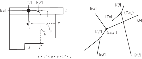
  Figure 13.

  If we can choose the $\kappa$-parameters such that $y_{i^{\prime},a,j}>y_{i,a,b,j}>y_{i,b,j^{\prime}}$ then it follows that there is an intersection of the $[a,j]$ and $[i,b]$ line-solitons in the contour plot.

  One simple choice is to require that

  (12.1) $$\kappa_{j} =-\kappa_{i}>0\quad\text{ and }\quad\kappa_{b}=-\kappa_{a}>0;\quad\text{ and also}$$

  (12.2) $$\kappa_{i^{\prime}} >\frac{1}{2}\kappa_{i}\quad\text{ and }\quad\kappa_{j^{\prime}}<\frac{1}{2}\kappa_{j}.$$

  By (12.1), we have $y_{i,a,b,j}=0$. By (12.2), together with $\kappa_{a}>\kappa_{i^{\prime}}$ and $\kappa_{b}<\kappa_{j^{\prime}}$, we have that

  $$y_{i^{\prime},a,j}=\kappa_{i^{\prime}}+\kappa_{a}+\kappa_{j}~{}>~{}0~{}>~{}\kappa_{i}+\kappa_{b}+\kappa_{j^{\prime}}=y_{i,b,j^{\prime}}.$$

  One concrete choice of parameters satisfying the required inequalities is $(\kappa_{i},\kappa_{i^{\prime}},\kappa_{a},\kappa_{b},\kappa_{j^{\prime}},\kappa_{j})=(-4r,-2r,-r,r,2r,4r)$ where $r>0$.
  

• The second case is that there is an empty box to the left of $b$ in $D^{\prime}$, and so the $[i,b]$ line-soliton has trivalent vertices at both ends. Figure 14 illustrates this situation. These vertices are the white vertex $v_{i,b,j^{\prime\prime}}$ and the black vertex $v_{i,b,j^{\prime}}$ where $i<i^{\prime}\leq a<b\leq j^{\prime}<j<j^{\prime\prime}$. As before, $[a,j]$ is an unbounded line-soliton at $y\ll 0$ which is incident to the trivalent vertex $v_{i^{\prime},a,j}$.

  

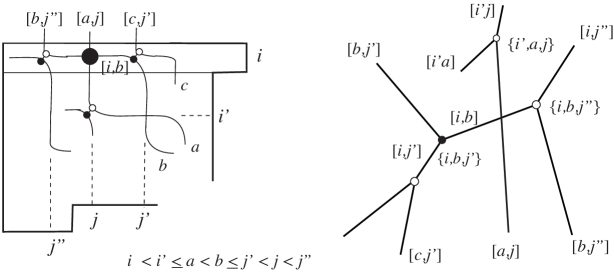
  Figure 14.

  Since $v_{i,b,j^{\prime\prime}}$ is a white vertex, if we can show that

  $$y_{i,b,j^{\prime\prime}}>y_{i,a,b,j}>y_{i,b,j^{\prime}},\qquad{\rm and}\qquad y_{i^{\prime}a,j}>y_{i,a,b,j},$$

  then it follows that the line-solitons of type $[a,j]$ and $[i,b]$ intersect in the contour plot.

  As before, we choose the $\kappa$-parameters so that (12.1) and (12.2) are satisfied. Then again we have $y_{i,a,b,j}=0$, $y_{i^{\prime},a,j}>0$, and $y_{i,b,j^{\prime}}<0$. Note that any choice of $\kappa_{j^{\prime\prime}}>\kappa_{j}$ gives $y_{i,b,j^{\prime\prime}}>0$, since $\kappa_{i}+\kappa_{b}+\kappa_{j^{\prime\prime}}>\kappa_{i}+\kappa_{b}+\kappa_{j}=\kappa_{b}>0$.

This completes the proof.        

12.2. Positivity of dominant exponentials and the proof of Theorem 12.1

In this section we prove Theorem 12.8 below. Once we have proved it, the proof of Theorem 12.1 will follow easily.

Theorem 12.8.

Let $A\in S_{D}\subset Gr_{k,n}$, where $D$ is a $\Gamma$ -diagram, and let $t\ll 0$. If $\Delta_{J}(A)>0$ for each dominant exponential $E_{J}$ in the contour plot $\operatorname{\mathcal{C}}_{t}(u_{A})$, then $A\in(Gr_{k,n})_{\geq 0}$. In other words, the Plücker coordinates corresponding to the dominant exponentials in $\operatorname{\mathcal{C}}_{t}(u_{A})$ comprise a positivity test for $S_{D}$.

Lemma 12.9.

Theorem 12.8 holds for elements $A\in Gr_{1,n}$.

Proof. Let $A\in S_{D}\subset Gr_{1,n}.$ If $D$ contains $r$ empty boxes, then $S_{D}$ has dimension $r$. Meanwhile, the element $A$ will have precisely $r+1$ nonzero Plücker coordinates. (We can normalize the lexicographically minimal one to be $1$.) It is easy to see that $G_{-}(D)$ and hence $\operatorname{\mathcal{C}}_{t}(u_{A})$ will have $r+1$ regions, each one labeled by a different dominant exponential corresponding to a Plücker coordinate $\Delta_{J}(A)$ such that $\Delta_{J}(A)\neq 0$. Therefore if each such $\Delta_{J}(A)>0$, then $A\in(Gr_{1,n})_{\geq 0}$.        

Lemma 12.10.

Let $A\in S_{D}\subset Gr_{k,n}$. Then it is possible to choose $\kappa_{1}<\kappa_{2}<\dots<\kappa_{n}$ such that the unbounded line-solitons at $y\ll 0$ in the corresponding contour plot $\operatorname{\mathcal{C}}_{t}(u_{A})$ (for any time $t$) appear in the same order as they do in the generalized plabic graph $G_{-}(D)$.

Proof. Recall that in a contour plot, the unbounded line-solitons $[i,j]$ at $y\ll 0$ appear from left to right in increasing order of the slope $\kappa_{i}+\kappa_{j}$. While in $G_{-}(D)$, one may easily check that the unbounded line-solitons $[i,j]$ at $y\ll 0$ appear from left to right in increasing order of $j$.

Now let us choose $\kappa_{1},\dots,\kappa_{n}$ so that $\kappa_{i}-\kappa_{i-1}=r^{i}$ for some constant $r>1$. To prove the lemma, it suffices to prove that given two line-solitons $[a,b]$ and $[c,d]$ at $y\ll 0$, where $b<d$, we have that

(12.3) $$\kappa_{a}+\kappa_{b}<\kappa_{c}+\kappa_{d},\text{ or equivalently, }\kappa_{d}-\kappa_{b}>\kappa_{a}-\kappa_{c}.$$

Since $a<b$ and $c<d$, we have $a<d$. By our choice of the $\kappa_{i}$’s, $\kappa_{d}-\kappa_{b}\geq r^{d}$. If $a<c$ then $\kappa_{a}-\kappa_{c}<0$, so (12.3) is obvious. On the other hand, if $a>c$, then $\kappa_{a}-\kappa_{c}\leq r^{a}+r^{a-1}+\dots+1<r^{a+1}.$ And since $a<d$, equation (12.3) follows.        

We now prove Theorem 12.8.

Proof. Our strategy is to use induction on the number of rows of $A$. Lemma 12.9 takes care of the base case of the induction. We suppose that $A$ is in row-echelon form, and let $A^{\prime}$ be the element of $Gr_{k-1,n}$ obtained from the bottom $k-1$ rows of $A$. Then $A^{\prime}\in S_{D^{\prime}}$ where $D^{\prime}$ is also a $\Gamma$ -diagram (it is the restiction of $D$ to its bottom $k-1$ rows). Recall from Theorem 10.14 that “most” of the contour plot $\operatorname{\mathcal{C}}_{t}(u_{A^{\prime}})$ is contained in the contour plot $\operatorname{\mathcal{C}}_{t}(u_{A})$. More precisely, every region of $\operatorname{\mathcal{C}}_{t}(u_{A^{\prime}})$ which is incident to a trivalent vertex and labeled by $E_{J^{\prime}}$ corresponds to a region of $\operatorname{\mathcal{C}}_{t}(u_{A})$ which is labeled by $E_{J^{\prime}\cup\{1\}}$. Because $A$ is in row-echelon form with a pivot in row $1$, $\Delta_{J^{\prime}\cup\{1\}}(A)=\Delta_{J^{\prime}}(A^{\prime})$, so the fact that each $\Delta_{J^{\prime}\cup\{1\}}(A)>0$ implies that $\Delta_{J^{\prime}}(A^{\prime})>0$.

We now claim that all Plücker coordinates corresponding to the dominant exponentials of the contour plot $\operatorname{\mathcal{C}}_{t}(u_{A^{\prime}})$ are positive. To prove this, note that from $\operatorname{\mathcal{C}}_{t}(u_{A})$ we can in fact construct $\operatorname{\mathcal{C}}_{t}(u_{A^{\prime}})$: all of the trivalent vertices of $\operatorname{\mathcal{C}}_{t}(u_{A^{\prime}})$ are present in $\operatorname{\mathcal{C}}_{t}(u_{A})$, so it is just a matter of extending some line-solitons that were finite in $\operatorname{\mathcal{C}}_{t}(u_{A})$ but are unbounded in $\operatorname{\mathcal{C}}_{t}(u_{A^{\prime}})$. These line-solitons may create some new white $X$-crossings but cannot create black $X$-crossings, because $D^{\prime}$ is a $\Gamma$ -diagram. If a single white $X$-crossing is created, then because three of its four regions are incident to a trivalent vertex, three of the four corresponding Plücker coordinates are positive. But then by the two-term Plücker relation relating the four Plücker coordinates, the fourth Plücker coordinate is positive as well. If multiple white $X$-crossings are created, then one can iterate the above argument, starting with a white $X$-crossing with three of its four regions incident to a trivalent vertex in the contour plot. This proves the claim. So by the inductive hypothesis, $A^{\prime}\in(Gr_{k-1,n})_{\geq 0}$.

Since $A^{\prime}\in(Gr_{k-1,n})_{\geq 0}$, it follows that all the Plücker coordinates labeling the regions of $G_{-}(D^{\prime})$ are positive. And so all of the Plücker coordinates labeling the regions of $G_{-}(D)$ which correspond to the bottom $k-1$ rows of $D$ are positive. (Recall again that $\Delta_{J^{\prime}\cup\{1\}}(A)=\Delta_{J^{\prime}}(A^{\prime})$.) If we can show that the Plücker coordinates labeling the regions of $G_{-}(D)$ which come from the top row of $D$ are positive, then by Remark 10.5, it will follow that $A\in(Gr_{k,n})_{\geq 0}$.

By Lemma 12.10, we can deform the $\kappa$-parameters so that the resulting contour plot $\operatorname{\mathcal{C}}^{\prime}_{t}(u_{A})$ has its unbounded line-solitons at $y\ll 0$ in the same order as those in $G_{-}(D)$. Then the dominant exponentials at $y\ll 0$ in $\operatorname{\mathcal{C}}^{\prime}_{t}(u_{A})$ are precisely those of $G_{-}(D)$, which in turn come from the top row of $D$. By Corollary 11.9, since the dominant exponentials of $\operatorname{\mathcal{C}}_{t}(u_{A})$ are positive, so are those of $\operatorname{\mathcal{C}}^{\prime}_{t}(u_{A})$. In particular, the dominant exponentials of $\operatorname{\mathcal{C}}^{\prime}_{t}(u_{A})$ at $y\ll 0$ are positive, so we can conclude that all of the Plücker coordinates labeling the regions of $G_{-}(D)$ are positive. Therefore $A\in(Gr_{k,n})_{\geq 0}$.        

Finally we are ready to prove Theorem 12.1.

Proof. Recall the definition of $u_{A}(x,y,t)$ in terms of the $\tau$-function from Section 6.2. It is easy to verify that if $A\in(Gr_{k,n})_{\geq 0}$, then $u_{A}(x,y,t)$ is regular for all times $t$: the reason is that $\tau_{A}(x,y,t)$ is strictly positive, and hence its logarithm is well-defined.

Conversely, let $A\in Gr_{k,n}$, and suppose that $u_{A}(x,y,t)$ is regular for $t\ll 0$. This means that the Plücker coordinates $\Delta_{J}$ corresponding to the dominant exponentials in the contour plot $\operatorname{\mathcal{C}}_{t}(u_{A})$ must all have the same sign. Since the Grassmannian is a projective variety, we may assume that all of these Plücker coordinates are positive.

Let $S_{D}$ be the Deodhar stratum containing $A$. If $D$ has a black stone, then by Theorem 12.7, the contour plot $\operatorname{\mathcal{C}}_{-\infty}(u_{A})$ contains a black $X$-crossing. But then by Corollary 11.6, two dominant exponentials incident to that black $X$-crossing must have opposite signs, which is a contradiction. Therefore we conclude that $D$ has no black stones. It follows that the Deodhar diagram corresponding to $D$ is a $\Gamma$ -diagram. But now by Theorem 12.8, it follows that $A\in(Gr_{k,n})_{\geq 0}$.

Finally, note that if $A\in Gr_{k,n}$ and $u_{A}(x,y,t)$ is regular for all times $t$, then in particular it is regular for $t\ll 0$, so the arguments of the previous two paragraphs apply. Therefore $A\in(Gr_{k,n})_{\geq 0}$.        

Remark 12.11.

Corollary 11.6 implies that there are singularities among the line-solitons forming a black $X$-crossing in a contour plot, and the singular solitons form a V-shape.

Example 12.12.

We revisit the example from Figures 5 and 10. Note that the contour plot at the left of Figure 10 is topologically identical to $G_{-}(D)$. The Go-diagram and labeled Go-diagram are as follows.

      

The $A$-matrix is given by

$$A=\begin{pmatrix}p_{11}p_{14}&p_{14}&0&0&1&0&0&0\\ 0&-p_{7}p_{8}p_{9}&-p_{8}p_{9}&-p_{9}&-m_{10}&0&-1&0\\ 0&0&0&-p_{4}&-m_{6}&1&0&0\\ 0&0&0&0&p_{3}&0&0&1\end{pmatrix}.$$

Recall from Theorem 5.6 that we associate a Plücker coordinate $\Delta_{I_{b}}$ to each box $b$ of the Go-diagram, via $I_{b}=v^{\rm in}(w^{\rm in})^{-1}\{1,2,4,5\}=\{j_{1},j_{2},j_{3},j_{4}\}$. For brevity, we simply write $(j_{1}j_{2}j_{3}j_{4})$ below. Because the contour plot at the left of Figure 10 is topologically identical to $G_{-}(D)$, all of these Plücker coordinates $\Delta_{I_{b}}$ correspond to dominant exponentials in the contour plot.

   

The diagram at the right shows the values of the corresponding Plücker coordinates when we choose all $p_{j}=1$ (regardless of the choice of the $m_{j}$ parameters). Since only the Plücker coordinate $\Delta_{1,2,6,8}(A)=-1$ is negative, the singular line-solitons in the contour plot are precisely those at the boundary of the corresponding region; these line-solitons have types $[4,6]$, $[5,8]$, and $[2,7]$-types.

12.3. Non-uniqueness of the evolution of the contour plots for $t\gg 0$

Consider $A\in S_{D}\subset Gr_{k,n}$. If the contour plot $\operatorname{\mathcal{C}}_{-\infty}(D)$ is topologically identical to $G_{-}(D)$, then the contour plot has almost no dependence on the parameters $m_{j}$ from the parameterization of $S_{D}$. This is because the Plücker coordinates corresponding to the regions of $\operatorname{\mathcal{C}}_{-\infty}(D)$ (representing the dominant exponentials) are either among the collection of minors given in Theorem 5.6 (by Remark 10.5), or determined from these by a “two-term” Plücker relation. Note that the minors given in Theorem 5.6 are computed in terms of the parameters $p_{i}$ but have no dependence on the $m_{j}$’s.

Therefore it is possible to choose two different points $A$ and $A^{\prime}$ in $S_{D}\subset Gr_{k,n}$ whose contour plots for a fixed $\kappa_{1}<\dots\kappa_{n}$ and fixed $t\ll 0$ are identical (up to some exponentially small difference); we use the same parameters $p_{i}$ but different parameters $m_{j}$ for defining $A$ and $A^{\prime}$. However, as $t$ increases, those contour plots may evolve to give different patterns.

Consider the Deodhar stratum $S_{D}\subset Gr_{2,4}$, corresponding to

$${\bf w}=s_{2}s_{3}s_{1}s_{2}\text{ and }{\bf v}=s_{2}11s_{2}.$$

The Go-diagram and labeled Go-diagram are given by

$$\leavevmode\;\vbox{\hbox{\begin{picture}(20.0,20.0)(0.0,0.0) \put(0.0,2.0){\line(1,0){10.0}}\put(0.0,-8.0){\line(1,0){10.0}}\put(0.0,20.0){\line(0,-1){10.0}}\put(10.0,20.0){\line(0,-1){10.0}}\put(5.0,15.0){\makebox(0.0,0.0)[]{\hskip 11.38092pt\circle*{5.0}}} \put(10.0,2.0){\line(1,0){10.0}}\put(10.0,-8.0){\line(1,0){10.0}}\put(10.0,20.0){\line(0,-1){10.0}}\put(20.0,20.0){\line(0,-1){10.0}}\put(15.0,15.0){\makebox(0.0,0.0)[]{}} \put(0.0,1.0){\line(1,0){10.0}}\put(0.0,-9.0){\line(1,0){10.0}}\put(0.0,10.0){\line(0,-1){10.0}}\put(10.0,10.0){\line(0,-1){10.0}}\put(5.0,5.0){\makebox(0.0,0.0)[]{}} \put(10.0,1.0){\line(1,0){10.0}}\put(10.0,-9.0){\line(1,0){10.0}}\put(10.0,10.0){\line(0,-1){10.0}}\put(20.0,10.0){\line(0,-1){10.0}}\put(15.0,5.0){\makebox(0.0,0.0)[]{\hskip 11.38092pt\circle{5.0}}} \end{picture}}}\;\qquad\qquad\leavevmode\;\vbox{\hbox{\begin{picture}(20.0,20.0)(0.0,0.0) \put(0.0,2.0){\line(1,0){10.0}}\put(0.0,-8.0){\line(1,0){10.0}}\put(0.0,20.0){\line(0,-1){10.0}}\put(10.0,20.0){\line(0,-1){10.0}}\put(5.0,15.0){\makebox(0.0,0.0)[]{$-1$}} \put(10.0,2.0){\line(1,0){10.0}}\put(10.0,-8.0){\line(1,0){10.0}}\put(10.0,20.0){\line(0,-1){10.0}}\put(20.0,20.0){\line(0,-1){10.0}}\put(15.0,15.0){\makebox(0.0,0.0)[]{$p_{3}$}} \put(0.0,1.0){\line(1,0){10.0}}\put(0.0,-9.0){\line(1,0){10.0}}\put(0.0,10.0){\line(0,-1){10.0}}\put(10.0,10.0){\line(0,-1){10.0}}\put(5.0,5.0){\makebox(0.0,0.0)[]{$p_{2}$}} \put(10.0,1.0){\line(1,0){10.0}}\put(10.0,-9.0){\line(1,0){10.0}}\put(10.0,10.0){\line(0,-1){10.0}}\put(20.0,10.0){\line(0,-1){10.0}}\put(15.0,5.0){\makebox(0.0,0.0)[]{$1$}} \end{picture}}}\;.$$

The matrix $g$ is calculated as $g=s_{2}y_{3}(p_{2})y_{1}(p_{3})x_{2}(m)s_{2}^{-1}$, and its projection to $Gr_{2,4}$ is

$$A=\begin{pmatrix}-p_{3}&-m&1&0\\ 0&p_{2}&0&1\end{pmatrix}.$$

The $\tau$-function is then given by

$$\tau_{A}=-(p_{2}p_{3}E_{1,2}+p_{3}E_{1,4}+mE_{2,4}+p_{2}E_{2,3}-E_{3,4}),$$

where $E_{i,j}:=(\kappa_{j}-\kappa_{i})\exp(\theta_{i}+\theta_{j})$. The contour plots of the solutions with $m=0$ and $m\neq 0$ are the same (except for some exponentially small difference) when $t\ll 0$. In both cases, the plot consists of two line-solitons forming an $X$-crossing, where the parts of those solitons adjacent to the region with dominant exponential $E_{3,4}$ (i.e. for $x\gg 0$) are singular, see the left of Figure 15.

On the other hand, for $t\gg 0$, the contour plot with $m=0$ is topologically the same as it was for $t\ll 0$, while the contour plot with $m\neq 0$ has a box with dominant exponential $E_{2,4}$, surrounded by four bounded solitons (some of which are singular). See the middle and right of Figure 15. So not only the contour plots but also the soliton graphs are different for $t\gg 0$!

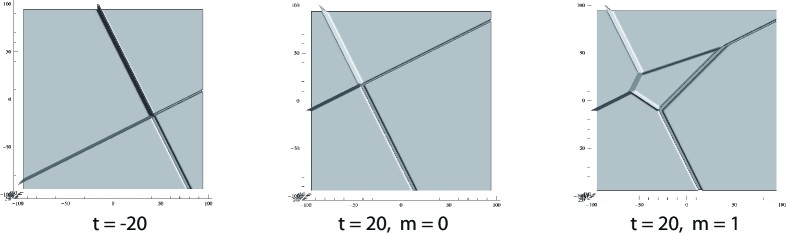
Figure 15. The non-uniqueness of the evolution of the contour plots (and soliton graphs). The left panel shows the contour plot at $t=-20$ for any value of $m$. The middle panel shows the graph at $t=20$ with $m=0$, and the right one shows the graph at $t=20$ with $m=1$. These contour plots were made using the choice $p_{i}=1$ for all $i$, and $(\kappa_{1},\ldots,\kappa_{4})=(-2,-1,0,1.5)$. In all of them, the region at $x\gg 0$ has a positive sign ($\Delta_{3,4}=1$) and other regions have negative signs. This means that the solitons adjacent to the region for $x\gg 0$ are singular.

Note that the non-uniqueness of the evolution of the contour plot (a tropical approximation) does not imply the non-uniqueness of the evolution of the solution of the KP equation as $t$ changes. If one makes two different choices for the $m_{i}$’s, the corresponding $\tau$-functions are different, but there is only an exponentially small difference in the corresponding contour plots (hence the topology of the contour plots is identical). This is particularly interesting to compare with the totally non-negative case, where the soliton solution can be uniquely determined by the information in the contour plot at $t\ll 0$. For more details, see the results on the inverse problem in [21].

References

- [1] M. J. Ablowitz, P. A. Clarkson, Solitons, nonlinear evolution equations and inverse scattering (Cambridge University Press, Cambridge, 1991)
- [2] G. Biondini, S. Chakravarty, Soliton solutions of the Kadomtsev-Petviashvili II equation, J. Math. Phys., 47 (2006) 033514 (26pp).
- [3] G. Biondini, Y. Kodama, On a family of solutions of the Kadomtsev-Petviashvili equation which also satisfy the Toda lattice hierarchy, J. Phys. A: Math. Gen. 36 (2003), 10519–10536.
- [4] A. Bjorner, F. Brenti, Combinatorics of Coxeter groups, Graduate Texts in Mathematics, 231, Springer, New York, 2005.
- [5] S. Chakravarty, Y. Kodama, Classification of the line-solitons of KPII, J. Phys. A: Math. Theor. 41 (2008) 275209 (33pp).
- [6] S. Chakravarty, Y. Kodama, A generating function for the N-soliton solutions of the Kadomtsev-Petviashvili II equation, Contemp. Math., 471 (2008), 47–67.
- [7] S. Chakravarty, Y. Kodama, Soliton solutions of the KP equation and applications to shallow water waves, Stud. Appl. Math. 123 (2009) 83–151.
- [8] V. Deodhar, On some geometric aspects of Bruhat orderings I. A finer decomposition of Bruhat cells, Invent. Math. 79 (1985), no. 3, 499–511.
- [9] V. Deodhar, On some geometric aspects of Bruhat orderings II. The parabolic analogue of Kazhdan-Lusztig polynomials, J. Alg. 111 (1987), 483–506.
- [10] L. A. Dickey, Soliton equations and Hamiltonian systems, Advanced Series in Mathematical Physics, Vol. 12, (World Scientific, Singapore, 1991).
- [11] O. Dudas, Note on the Deodhar decomposition of a double Schubert cell, arXiv:0807.2198.
- [12] N. Freeman, J. Nimmo, Soliton-solutions of the Korteweg-deVries and Kadomtsev-Petviashvili equations: the Wronskian technique, Phys. Lett. A 95 (1983), 1–3.
- [13] R Hirota, The Direct Method in Soliton Theory (Cambridge University Press, Cambridge, 2004)
- [14] B. B. Kadomtsev, V. I. Petviashvili, On the stability of solitary waves in weakly dispersive media, Sov. Phys. - Dokl. 15 (1970) 539-541.
- [15] D. Kazhdan, G. Lusztig, Representations of Coxeter groups and Hecke algebras, Invent. Math. 53 (1979), no. 2, 165–184.
- [16] D. Kazhdan, G. Lusztig, Schubert varieties and Poincaré duality, Geometry of the Laplace operator (Proc. Sympos. Pure Math., Univ. Hawaii, Honolulu, Hawaii, 1979), Proc. Sympos. Pure Math., XXXVI, Amer. Math. Soc., Providence, R.I., 1980, pp. 185–203. MR 84g:14054
- [17] A. Knutson, T. Lam, D. Speyer, Positroid varieties: juggling and geometry, arXiv:1111.3660.
- [18] Y. Kodama, Young diagrams and -soliton solutions of the KP equation, J. Phys. A: Math. Gen., 37 (2004) 11169-11190.
- [19] Y. Kodama, KP solitons in shallow water, J. Phys. A: Math. Theor. 43 (2010) 434004 (54pp).
- [20] Y. Kodama, L. Williams, KP solitons, total positivity, and cluster algebras, Proc. Natl. Acad. Sci. USA 108 (2011), no. 22, 8984–8989.
- [21] Y. Kodama, L. Williams, KP solitons and total positivity for the Grassmannian, arXiv:1106.0023.
- [22] T. Lam, L. Williams, Total positivity for cominuscule Grassmannians, New York J. Math., 14 (2008), 53-99.
- [23] G. Lusztig, Total positivity in partial flag manifolds, Representation Theory, 2 (1998) 70-78.
- [24] R. Marsh, K. Rietsch, Parametrizations of flag varieties, Representation Theory, 8 (2004) 212-242.
- [25] T. Miwa, M. Jimbo, E. Date, Solitons: differential equations, symmetries and infinite-dimensional algebras (Cambridge University Press, Cambridge, 2000)
- [26] S. Novikov, S. V. Manakov, L. P. Pitaevskii, V. E. Zakharov, Theory of Solitons: The Inverse Scattering Method, Contemporary Soviet Mathematics, (Consultants Bureau, New York and London, 1984).
- [27] J. G. Oxley, Matroid theory, Oxford University Press, New York, 1992.
- [28] A. Postnikov, Total positivity, Grassmannians, and networks, http://front.math.ucdavis.edu/math.CO/0609764.
- [29] R. Proctor, Bruhat lattices, plane partition generating functions, and minuscule representations. European J. Combin. 5 (1984), no. 4, 331–350.
- [30] K. Rietsch, Total positivity and real flag varieties, Ph.D. Dissertation, MIT, 1998.
- [31] M. Sato, Soliton equations as dynamical systems on an infinite dimensional Grassmannian manifold, RIMS Kokyuroku (Kyoto University) 439 (1981), 30–46.
- [32] J. Satsuma, A Wronskian representation of -soliton solutions of nonlinear evolution equations, J. Phys. Soc. Japan, 46 (1979) 356-360.
- [33] J. Scott, Grassmannians and cluster algebras, Proc. London Math. Soc. (3) 92 (2006), 345–380.
- [34] J. Stembridge, On the Fully Commutative Elements of Coxeter Groups. J. Algebraic Combinatorics 5 (1996), 353–385.
- [35] K. Talaska, L. Williams, Network parameterizations of Grassmannians, to appear in Alg. Numb. Theory.
- [36] L. Williams, Shelling totally nonnegative flag varieties, J. Reine Angew. Math. 609 (2007), 1–21.