Selecting Quasar Candidates by a SVM Classification System

Abstract

We develop and demonstrate a classification system constituted by several Support Vector Machines (SVM) classifiers, which can be applied to select quasar candidates from large sky survey projects, such as SDSS, UKIDSS, GALEX. How to construct this SVM classification system is presented in detail. When the SVM classification system works on the test set to predict quasar candidates, it acquires the efficiency of 93.21% and the completeness of 97.49%. In order to further prove the reliability and feasibility of this system, two chunks are randomly chosen to compare its performance with that of the XDQSO method used for SDSS-III’s BOSS. The experimental results show that the high faction of overlap exists between the quasar candidates selected by this system and those extracted by the XDQSO technique in the dereddened i-band magnitude range between 17.75 and 22.45, especially in the interval of dereddened i-band magnitude $<$ 20.0. In the two test areas, 57.38% and 87.15% of the quasar candidates predicted by the system are also targeted by the XDQSO method. Similarly, the prediction of subcategories of quasars according to redshift achieves a high level of overlap with these two approaches. Depending on the effectiveness of this system, the SVM classification system can be used to create the input catalog of quasars for the GuoShouJing Telescope (LAMOST) or other spectroscopic sky survey projects. In order to get higher confidence of quasar candidates, cross-result from the candidates selected by this SVM system with that by XDQSO method is applicable.

1 Introduction

Over the years, the volume of astronomical data at different wavebands grows dramatically with large space-based and ground-based telescopes surveying the sky, such as SDSS, 2MASS, NVSS, FIRST and 2dF. How to preselect scientific targets from the enormous amount of observed data is a significant and challenging issue. In another words, how to extract knowledge from a huge volume of data by automated methods is an important task for astronomers. In the next decade, the ongoing or planned multiband photometric survey projects, for instance, the Large Synoptic Survey Telescope (LSST; Tyson 2002), the Visible and Infrared Survey Telescope for Astronomy (VISTA; McPherson et al. 2006), and the Panoramic Survey Telescope and Rapid Response System (Pan-STARRS; Kaiser et al. 2002) will bring more serious challenges for astronomers.

Ball and Brunner (2009) reviewed the current state of data mining and machine learning in astronomy. Borne (2009) also described the application of data mining algorithms to research problems in astronomy. A lot of Data Mining (DM) algorithms have been applied to find quasar candidates in astronomy. Traditional quasar selection relies on cutoff in a two-dimensional color space although most modern surveys are done in several bandpasses. Traditional methods can’t make use of the provided information from the high dimensional space. Otherwise, the DM approaches utilize the features as many as possible. In general, DM methods for quasar candidate selection can be divided into two types: supervised and unsupervised learning. Most methods used in this domain of astronomy belong to supervised learning. Abraham et al. (2010) used a Difference Boosting Neural Network (DBNN) classifier which is a bayesian supervised learning algorithm to make a catalogue of quasar candidates from the Sloan Digital Sky Survey Seventh Data Release (SDSS DR7; Abazajian et al. 2009). Carballo et al. (2008) obtained a sample set of redshift $\geq$ 3.6 radio quasi-stellar objects using Neural Network (NN). Quasar candidate detection also can be achieved by using unsupervised clustering algorithms in color spaces, such as the Probabilistic Principal Surface(PPS) algorithm (D’Abrusco, Longo & Walton 2009). The most representative work could be the series of work completed by the SDSS team until now, especially for the SDSS-III Baryon Oscillation Spectroscopic Survey (BOSS; Schlegel et al. 2007; Eisenstein et al. 2011). Ross et al. (2011) gave a flowchart for the BOSS quasar target selection and exploited several methods including an Extreme-Deconvolution method (XDQSO; Bovy et al. 2011), a Kernel Density Esitimator (KDE; Richards et al. 2004, 2009), a Likelihood method which likes KDE (Kirkpatrick et al. 2011) and a Neural Network method (NN; Yèche et al. 2010) in this flowchart. After several times comparisons of the efficiency of quasar selection methods, XDQSO was declared to be CORE for the rest of the BOSS quasar survey.

Support Vector Machines (SVM) is a supervised learning method and it can produce a non-probabilistic binary linear classifier given a set of training examples each of which is labeled as one of two categories. SVM provides a good out-of-sample generalization and can be robust, even when the training sample has some bias. This distinguishing feature of SVM attracts many astronomers to use it for selecting quasar candidates. Zhang & Zhao (2003) applied two classification algorithms, Support Vector Machines (SVM) and Learning Vector Quantization (LVQ), to study the distribution of various astronomical sources in the multidimensional parameter space. Zhang & Zhao (2004) demonstrated that SVM can show better performance than Learning Vector Quantization (LVQ) and Single-Layer Perceptron (SLP) when preselecting AGN candidates. Gao et al. (2008) compared the performance of SVM with K-Dimensional Tree (KD-Tree) to separate quasars from stars and provide a good parameter combination of magnitudes and colors for SVM. Bailer-Jones et al. (2008) developed and demonstrated a probabilistic method for classifying quasars in surveys, named the Discrete Source Classifier (DSC) which is a supervised classifier based on SVM. Kim et al. (2011) presented how to use SVM to do a variability selection for quasars on a set of extracted time series features including period, amplitude, color and autocorrelation value. In this work, we focus on constructing a kind of classification system based SVM and use it to select quasar candidates for the Chinese GuoShouJing Telescope (LAMOST).

This paper is organized as follows. Section 2 describes the characteristics of data used in this experiment in detail. In Section 3, we presents the brief of SVM, and how to use it to construct a SVM classification system. Section 4 demonstrates the performance of this method for separating quasars from stars in a test set. The comparison of this system with the XDQSO method for classifying quasars and stars will be discussed in Section 5. In Section 6, we give the conclusion about our method and what should be improved in the future work.

2 The Data

The Sloan Digital Sky Survey (SDSS) is one of the most ambitious and influential surveys in the history of astronomy (York et al. 2000). The SDSS used a dedicated 2.5-meter telescope at Apache Point Observatory, New Mexico, equipped with two powerful special-purpose instruments. The 120-megapixel camera imaged 1.5 square degrees of sky at a time, about eight times the area of the full moon. Over eight years of operations (SDSS-I, 2000-2005; SDSS-II, 2005-2008), it obtained deep, multi-color images covering more than a quarter of the sky and created 3-dimensional maps containing more than 930,000 galaxies and more than 120,000 quasars. Meanwhile, SDSS is continuing with the Third Sloan Digital Sky Survey (SDSS-III), a program of four new surveys using SDSS facilities. SDSS-III began observations in July 2008 and released its first public data as Data Release 8 to emphasize its continuity with previous SDSS releases. SDSS-III will continue operating and releasing data through 2014. SDSS-II carried out three distinct surveys: the Sloan Legacy Survey, SEGUE (the Sloan Extension for Galactic Understanding and Exploration), the Sloan Supernova Survey. SDSS-III builds on the legacy of the SDSS and SDSS-II to generate high-quality scientific data and to make important new discoveries. SDSS-III has been designed to maximize understanding of three scientific themes: Dark energy and cosmological parameters, the structure, dynamics, and chemical evolution of the Milky Way, the architecture of planetary systems.

The creation of a good classifier depends on a complete and representive training sample. Therefore careful preparation of training sample is of great importance. In this specific problem, we just care about separating quasars from stars and thus exclude extended sources (GALAXY). The training sets and test sets used in this method are produced from four data sets Quasar Catalogue V (Schneider et al. 2010), SDSS DR7 (Abazajian et at. 2009), SDSS DR8(Aihara et al. 2011) and SDSS-XDQSO (Bovy et al. 2011). In this section, we simply introduce these four data sets and how to use them to construct the training set for each SVM classifier in detail will be discussed in Section 3.2.

Based upon the SDSS DR7, quasar Catalogue V contains 105,783 (LowZ_No 88201, MedZ_No 14063, HighZ_No 3519) spectroscopically confirmed quasars and represents the conclusion of the SDSS-I and SDSS-II quasar survey. In the following, LowZ_QSO, MedZ_QSO and HighZ_QSO are short for low-redshift quasars, medium-redshift quasars and high-redshift quasars, respectively. According to the paper (Bovy et al. 2011), the definition of low-redshift, medium-redshift and high-redshift corresponds to $z<2.2$, $2.2\leq z\leq 3.5$ and $z>3.5$, separately. For the several training sets in our SVM classification system, nine tenths of quasars (95,202 quasars including 79,421 LowZ_QSO, 12,610 MedZ_QSO and 3,171 HighZ_QSO) of this catalogue are randomly sampled to construct them and the remaining one tenth of quasars (10,581 quasars including 8,780 LowZ_QSO, 1,453 MedZ_QSO and 348 HighZ_QSO) will be used as test samples of quasars.

The training sample of stars consists of three parts. The first part is from the spectral confirmed stars of SDSS DR8, the second part comes from the unidentified pointed sources with psfMag_i $<17.75$ in the subarea of Stripe-82, the third part is made up of the pointed sources with deredened $i$-band magnitude between 17.75 and 22.45 mag in the same subarea of Stripe-82 removing those predicted by SDSS-XDQSO as quasars (the probability of quasars $>0.5$). The detailed information about the three parts is described as follows.

The spectral confirmed stars used in training sets are produced from SpecPhotoAll Table in SDSS DR8 using the SQL interface to Catalog Archive Server (CAS) mainly following the criteria described in Section 3.2.1 of Richards et al. 2002. Some records in the SpecPhotoAll Table of SDSS DR8 should be removed because the sky survey plan makes some sources to be duplicately observed several times and some spectroscopically identified objects don’t have photometric corresponding sources. We set the attribute class $=STAR$ which means this record is a stellar object, sciencePrimary $=1$ which represents the best version of spectrum at this location, Mode $=1$ which denotes this record with the best photometric data and zWarrning $=0$ to ensure the subclass of STAR more reliable. The records with fatal errors are excluded using flags such as BRIGHT, SATURATED, EDGE and BLENDED. We also reject the objects whose magnitude errors are larger than 0.2 in all five optical bands. In addition, a very few records with the same objID are weeded out. Finally, we get a catalog of 480,878 spectral confirmed stars from SpecPhotoAll Table of SDSS DR8 and randomly sampled out two thirds (No. 320584) of them for training and the rest (No. 160,294) of them for test.

The sample of photometric stars without spectra is constructed from the PhotoObjAll table in SDSS DR8 using mode $=1$, type $=6$, specObjID $=0$ and psfMag_i $<17.75$. Since SDSS Stripe-82 (Abazajian et al. 2009) has been observed many times, the data from this area are reliable. The point sources in this area with the psfMag_i $<17.75$ can rarely be quasars, so these photometric sources are regarded as stars. Actually, we select a subarea which covers 150 deg² (-$30^{\circ}<\alpha_{\mathrm{J2000}}<+30^{\circ}$ and -$1^{\circ}.25<\delta_{\mathrm{J2000}}<+1^{\circ}.25$) and this area was also chosen by SDSS-XDQSO (Bovy et al. 2011). Consequently, these are 115,010 photometric stars in this subarea of Stripe-82 with the psfMag_i $<17.75$.

SDSS-XDQSO method is one of methods which serve SDSS-III for targeting quasars. It uses the extreme-deconvolution method to estimate the underlying density of stars and quasars in flux space and then it convolves this density with flux uncertainties when evaluating the probability that an unknown object is a quasar. In recent blind tests of SDSS-III, it demonstrates a good performance to the faint objects. SDSS-XDQSO quasar targeting catalog contains 160,904,060 point-sources with dereddened $i$-band magnitude between 17.75 and 22.45 mag in the 14,555 $deg^{2}$ of imaging from SDSD DR8. For our training sets, we just select the objects (No. 301,043) in the subarea of Stripe-82 except those predicted as quasars by SDSS-XDQSO (the probability of quasars $>0.5$).

The test set are composed of two parts. The first one is one tenth (No. 95,202) of quasar Catalogue V and the second one is one thirds (No. 160,294) of SpecPhotoAll table in SDSS DR8 which has been cleaned in the above paragraph.

3 METHOD

3.1 SVM

Support Vector Machines (SVM), proposed by Vapnik (1995), is derived from the theory of structural risk minimization which belongs to statistical learning theory. The core idea of SVM is to map input vectors into a high-dimensional feature space and construct the optimal separating hyperplane in this space. SVM aims at minimizing an upper bound of the generalization error through maximizing the margin between the separating hyperplane and the data. Basically, we are looking for the optimal separating hyperplane between the two classes by maximizing the margin between the classes’ closest points. In Figure 1 points lying on the boundaries are called support vectors and it means that SVM just uses the most representative points to construct a classifier not using all of them.

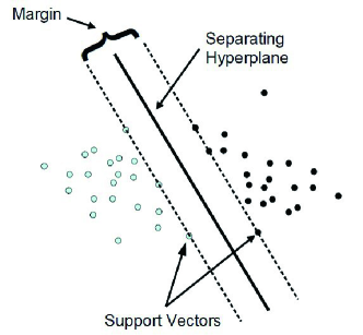
Figure 1: This is a linear separable case of SVM.

For a given training set belonging to two different classes is often called positive class and negative class (or plus class and minus class),

$$T={(\vec{x}_{1},y_{1}),\ldots,(\vec{x}_{n},y_{n})},\qquad\vec{x}_{i}\in\mathbf{R^{N}},y_{i}\in{\{-1,+1\}}$$ (1)

SVM learns linear threshold functions of the type.

$$h(\vec{x}_{i})=sign\{\vec{\omega}\cdot\vec{x}_{i}+b\}=\left\{\begin{aligned} +1,&~{}~{}~{}\mbox{if}~{}~{}~{}\vec{\omega}\cdot\vec{x}_{i}+b>0\\ -1,&~{}~{}~{}\mbox{else}\end{aligned}\right.$$ (2)

Each linear threshold function corresponds to a hyperplane in a feature space and the side of the hyperplane on which an example $\vec{x}_{i}$ lies determines the classified result by the function $h(\vec{x}_{i})$. If the training data can be separated by at least one hyperplane $h^{\prime}$, the optimal hyperplane with maximum margin can be found by minimizing

$$F(\vec{\omega},\vec{\xi})=\frac{1}{2}(\vec{\omega}\cdot\vec{\omega})+C\sum_{i=1}^{n}\xi_{i}$$ (3)

which subjects to

$$y_{i}[(\vec{\omega}\cdot\vec{x}_{i})+b]\geq 1-\xi_{i}\qquad i=1,\ldots,n$$ (4)

$$\xi_{i}>0\qquad i=1,\ldots,n$$ (5)

The factor $C$ is used to trade off training error against model complexity and $\xi$ are slack variables responding to the wrong prediction. In practice, we would like to penalize the errors on positive examples (quasars) stronger than errors on negative examples (stars), because we are much more interested in quasars than stars and the quantity of stars is often much larger than that of quasars. Morik et al. (1999) modified the Eq. 3 through minimizing

$$F(\vec{\omega},\vec{\xi})=\frac{1}{2}(\vec{\omega}\cdot\vec{\omega})+C_{-+}\sum_{i:y_{i}=+1}\xi_{i}+C_{+-}\sum_{j:y_{j}=-1}\xi_{j}$$ (6)

which is constrained by

$$y_{i}[(\vec{\omega}\cdot\vec{x}_{i})+b]\geq 1-\xi_{k}\qquad k=1,\ldots,n$$ (7)

We can use the both factors $C_{-+}$ and $C_{+-}$ to control the cost of false positives versus false negatives and get the result that we focus on. The books (Vapnik 1995; Vapnik 1998) contain excellent description of SVM and the article written by Burges (1998) provides a good tutorial on it. In this paper, we adopt $SVM^{light}$ coded by Joachims (2002) which is an implementation of SVM in C language with many extensional and additional softwares, moreover this code provides various model parameters including kernel functions for us to tune.

3.2 Build a SVM classification system

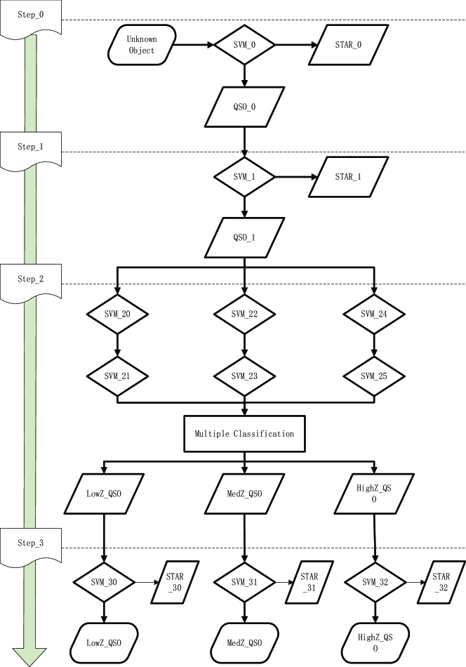
Figure 2: The scheme of a SVM classification system. A total of eleven classifiers (SVM_0, SVM_1, SVM_20, SVM_21, SVM_22, SVM_23, SVM_24, SVM_25, SVM_30, SVM_31 and SVM_32) for separating quasars from stars are trained by SVM. After being processed by these classifiers, any unknown sample will be classified in one of the four categories, namely LowZ_QSO, MedZ_QSO, HighZ_QSO and stars ( STAR_0, STAR_1, STAR_2, STAR_30, STAR_31 and STAR_32).

In this chapter, we discuss how to use several SVM models to build a SVM classification system for selecting quasar candidates in detail. The input pattern of SVM is a combination of photometric magnitudes and colors, just like the combination (psfMag_u-psfMag_g, psfMag_g-psfMag_r, psfMag_r-psfMag_i, psfMag_i-psfMag_z, psfMag_r) mentioned in Gao et al. (2008). All magnitudes in this combination have been corrected by the map of Schlegel et al. (1998). In Figure 2, we give the scheme of the SVM classification system with four steps and eleven models. Although many data mining algorithms have been successfully applied on this problem, most of them solved it only with one classifier. Actually this is very hard for one model to include all information at the same time and limits the performance of a classifier. Our idea is that we divide this task into several relative simple subtasks and conquer them respectively. The work of Step_0 (SVM_0) is about eliminating the stars that are apparently different from quasars. Step_1 (SVM_1) is mainly to separate quasars from the confusing stars. These two steps are the foundation of this system and many other authors combine the both together or just deal with one of them. The duty of Step_2 (from SVM_20 to SVM_25) is to divide the quasar candidates into three subclasses. Finally, Step_3 (SVM_30, SVM_31 and SVM_32) can make a further clean of the quasar candidates of each subclass and improve the prediction accuracies of the subclasses much higher.

For constructing the classifier of SVM_0, the above mentioned training samples of stars and quasars in Section 2 will be used to build a classifier. The training samples of stars are adopted from two thirds of spectroscopically confirmed stars in SDSS DR8, photometric stars in SDSS DR8 with dereddened $i$-band magnitude $<17.75$, photometric stars in SDSS-XDQSO with dereddened $i$-band magnitude between 17.75 and 22.45 and the probability-XDQSO less than 0.5. Nine tenths of spectral identified quasars in Schneider’s Catalog V are randomly sampled and taken as the training sample of quasars. Considering the small sample of quasars, we don’t put constraint on quasars in the scope of the subarea of Stripe-82. Generally when the completeness is higher, the efficiency is lower. Since our primary goal in this session is to weed out most stars (i.e. STAR_0) which are apparently different from quasars and easy to be eliminated, the low efficiency can be accepted. In Table 1, we list all training sets used in each classifier. Many confusing stars will be mixed into our quasar candidates (QSO_0) of SVM_0 in this step but we reserve quasars as many as possible.

Table 1: The number of training data used in each SVM model. Positive and negative separately denote what role played by the corresponding quasars or stars for constructing a classifier. From SVM_20 to SVM_25 just use quasars as the positive and negative samples because their functions are to classify quasar candidates into the three subcategories: LowZ_QSO, MedZ_QSO and HighZ_QSO.

Model	Positive (QSO)	Negative (Star)
	No.	No.
SVM_0	95,202	442,309
SVM_1	93,773	6,474
SVM_30	79,635	1,381
SVM_31	10,396	95
SVM_32	3,001	105
	LowZ_QSO	MedZ & HighZ_QSO
	No.	No.
SVM_20	79,421	15,781
	MedZ_QSO	HighZ_QSO
	No.	No.
SVM_21	12,610	3,171
	MedZ_QSO	LowZ & HighZ_QSO
	No.	No.
SVM_22	12,610	82,529
	LowZ_QSO	HighZ_QSO
	No.	No.
SVM_23	79,421	3,171
	HighZ_QSO	LowZ & MedZ_QSO
	No.	No.
SVM_24	3,171	92,031
	LowZ_QSO	MedZ_QSO
	SV No.	SV No.
SVM_25	79,421	12,610

After getting the SVM_0 model, we use it to process the data set composed of two thirds of spectroscopically identified stars in SDSS DR8 and nine tenths of quasars in Schneider’s QSO Catalogue V. The objects labeled as quasar candidates (QSO_0) by SVM_0 contain most of genuine quasars (No. 94,603) and many confusing stars (No. 6,474). These objects will be used to form the training set for SVM_1. We directly discard the objects marked as STAR_0 ( 314,110 stars and 599 quasars) by SVM_0 because the responsibility of SVM_1 is to distinguish the objects that can not be solved by SVM_0. When SVM_1 model is applied to QSO_0, many confusing stars will be removed out of it.

In order to divide the quasar candidates into three subclasses: LowZ_QSO (low-redshift quasars), MedZ_QSO (medium-redshift quasars) and HighZ_QSO (high-redshift quasars), there is a multiple classification with three branches needed to be built using nine tenths of quasars in Schneider’s QSO catalog V without adding any star sample. QSO_1 obtained by SVM_1 will be processed through three branches, each of them is a two-layer classifier and then the objects in QSO_1 will be marked as the subclass that gets the most votes. In Figure 2, for example, there are SVM_20 and SVM_21 in the first branch to discriminate LowZ_QSO, MedZ_QSO and HighZ_QSO. SVM_20 classifies LowZ_QSO from MedZ_QSO and HighZ_QSO and then SVM_21 distinguishes MedZ_QSO from HighZ_QSO. After processing by the two models, the quasar candidates will get a subcategory and the corresponding prediction value made by SVM. In the second branch, SVM_22 deals with MedZ_QSO vs. LowZ/HighZ_QSO and SVM_23 handles LowZ_QSO vs. HighZ_QSO. In the third branch, SVM_24 deals with HighZ_QSO vs. LowZ/MedZ_QSO and SVM_25 handles LowZ_QSO vs. MedZ_QSO. When the object gets the same vote with LowZ_QSO, MedZ_QSO and HighZ_QSO, the category with the maximum absolute SVM prediction value will be assigned to this object. The maximum absolute SVM prediction value of one quasar candidate means that it is farthest away from the optimal separate hyperplane and it is more likely to belong to this class.

Table 2: The number of support vectors (SV) used in each SVM model. Positive denotes which type of objects marked as plus and negative denotes which type of objects marked as minus in a SVM model.

Model	Positive (QSO)	Negative (Star)
	SV No.	SV No.
SVM_0	3,641	3,849
SVM_1	5,480	5,424
SVM_30	1,494	1,381
SVM_31	168	95
SVM_32	167	105
	LowZ_QSO	MedZ & HighZ_QSO
	SV No.	SV No.
SVM_20	4,835	4,889
	MedZ_QSO	HighZ_QSO
	SV No.	SV No.
SVM_21	666	679
	MedZ_QSO	LowZ & HighZ_QSO
	SV No.	SV No.
SVM_22	4,145	4,195
	LowZ_QSO	HighZ_QSO
	SV No.	SV No.
SVM_23	665	662
	HighZ_QSO	LowZ & MedZ_QSO
	SV No.	SV No.
SVM_24	442	439
	LowZ_QSO	MedZ_QSO
	SV No.	SV No.
SVM_25	4,835	4,828

The remaining three SVM models are SVM_30, SVM_31 and SVM_32. Their functionalities are to eliminate some very indistinguishable stars from LowZ_QSO, MedZ_QSO and HighZ_QSO, respectively. The main idea is that when quasar candidates selected out by SVM_0 and SVM_1, the classifiers utilize the general characteristics of quasars and stars. In the subcategory, we can make use of its own characteristics to get a more pure quasar set. Therefore, the training sets for the three models are based on the positive class (QSO_1) extracted from the data set composed of two thirds of spectroscopically identified stars in SDSS DR8 and nine tenths of quasars in Schneider’s QSO Catalogue V processed by SVM_0 and SVM_1 and then this positive class will be divided into three segments by multiple classification. The three segments will be used for generating SVM_30, SVM_31 and SVM_32 separately and each of them includes some indistinguishable stars that can not be simply weeded out by SVM_0 and SVM_1. Through these three models, a small amount of star contaminants is removed. It is also noticed that the risk of misclassifying a number of genuine quasars into star contaminants exists especially for high-redshift quasars.

In Table 2, we list the number of support vectors used in each of the SVM models. Obviously SVM does not need to use all samples to construct a classifier because it only uses the samples located on the optimal separating hyperplane in a high-dimensional feature space. The number of support vectors reflects the complexity of the problem solved by a classifier. Although the training set of SVM_0 is the largest one, the number of support vectors is small because most of stars can be easily separated from quasars. The most hard work belongs to SVM_1 and this model includes 5,480 quasars and 5,424 stars as support vectors because many quasars and stars are very similar even in a high-dimensional feature space.

4 THE PERFORMANCE OF SVM

Table 3: The evaluation of the ability of SVM for predicting the quasar subclasses: LowZ_QSO, MedZ_QSO and HighZ_QSO using the test quasar samples retained in QSO_1. The number 8543 shows how many true low-redshift quasars are correctly predicted in LowZ_QSO. The value 97.25% represents the efficiency (E.) of predicted LowZ_QSO to true low-redshift quasars. The value 98.66% denotes the completeness (C.) of true low-redshift quasars in all predicted quasar sample.

Predicted Class	True LowZ_QSO			True MedZ_QSO			True HighZ_QSO
	No.	E.(%)	C.(%)	No.	E.(%)	C.(%)	No.	E.(%)	C.(%)
LowZ_QSO	8543	97.25	98.66	242	2.75	18.11	0	0.00	0.00
MedZ_QSO	113	9.37	1.31	1083	89.80	81.06	10	0.83	3.12
HighZ_QSO	3	0.93	0.03	11	3.40	0.82	310	95.68	96.88

Table 4: The number and the fraction of stars mixed into our predicted categories LowZ_QSO, MedZ_QSO and HighZ_QSO, respectively. The column test (No.) shows the number of stars that would be used to test in our method. The column Step_0 (No.) means how many stars can not be removed by Step_0 of SVM. For A0 stars, the number 52 of A0 in LowZ_QSO indicates how many A0 stars finally can not be eliminated by Step_3. The decimal number 6.92 (i.e. 52/751) represents the contaminant percentage of A0 stars occupied in the whole contaminant sample set (751 stars can not be correctly classified by our method). The another decimal number 0.29 (i.e. 52/17953) means that this percentage of A0 stars in the whole A0 stars will be misclassified as LowZ_QSO. None of Carbon_lines stars mixed into any one of the three classes and we use ”–.–” to represent the percentage is null.

Star Subclass	Test	Step_0	LowZ_QSO			MedZ_QSO			HighZ_QSO
	No.	No.	Step_3 No.	P.(%)	P.(%)	Step_3 No.	P.(%)	P.(%)	Step_3 No.	P.(%)	P.(%)
A0	17953	349	52	6.92	0.29	15	2.00	0.08	0	0.00	0.00
A0p	348	6	3	0.40	0.86	0	0.00	0.00	0	0.00	0.00
B6	138	20	9	1.20	6.52	2	0.27	1.45	0	0.00	0.00
B9	200	13	4	0.53	2.00	1	0.13	0.50	0	0.00	0.00
CV	594	368	215	28.63	36.20	2	0.27	0.34	0	0.00	0.00
Carbon	79	5	1	0.13	1.27	0	0.00	0.00	0	0.00	0.00
CarbonWD	36	30	17	2.26	47.22	0	0.00	0.00	0	0.00	0.00
Carbon_lines	195	36	0	–.–	–.–	0	–.–	–.–	0	–.–	–.–
F2	4170	19	0	0.00	0.00	1	0.13	0.02	0	0.00	0.00
F5	27888	180	10	1.33	0.04	11	1.46	0.04	0	0.00	0.00
F9	34262	133	0	0.00	0.00	5	0.67	0.01	1	0.13	0.00
G0	3289	13	0	0.00	0.00	2	0.27	0.06	0	0.00	0.00
G2	8399	39	1	0.13	0.01	6	0.80	0071	0	0.00	0.00
G5	1	0	0	–.–	–.–	0	–.–	–.–	0	–.–	–.–
K1	8505	141	1	0.13	0.01	1	0.13	0.01	1	0.13	0.01
K3	8997	365	3	0.40	0.03	2	0.27	0.02	4	0.53	0.04
K5	7957	241	1	0.13	0.01	0	0.00	0.00	14	1.86	0.18
K7	5430	99	2	0.27	0.04	0	0.00	0.00	11	1.46	0.20
L0	18	0	0	–.–	–.–	0	–.–	–.–	0	–.–	–.–
L1	14	0	0	–.–	–.–	0	–.–	–.–	0	–.–	–.–
L2	41	0	0	–.–	–.–	0	–.–	–.–	0	–.–	–.–
L3	6	0	0	–.–	–.–	0	–.–	–.–	0	–.–	–.–
L4	9	0	0	–.–	–.–	0	–.–	–.–	0	–.–	–.–
L5	10	0	0	–.–	–.–	0	–.–	–.–	0	–.–	–.–
L5.5	56	9	4	0.53	7.14	1	0.13	1.79	0	0.00	0.00
L9	66	9	7	0.93	10.61	0	0.00	0.00	0	0.00	0.00
M0	3665	53	0	0.00	0.00	0	0.00	0.00	12	1.60	0.33
M0V	604	8	0	–.–	–.–	0	–.–	–.–	0	–.–	–.–
M1	3442	30	1	0.13	0.03	0	0.00	0.00	3	0.40	0.09
M2	4922	22	2	0.27	0.04	0	0.00	0.00	5	0.67	0.10
M2V	162	1	0	–.–	–.–	0	–.–	–.–	0	–.–	–.–
M3	4604	34	1	0.13	0.02	0	0.00	0.00	2	0.27	0.04
M4	3099	29	0	0.00	0.00	0	0.00	0.00	1	0.13	0.03
M5	1947	14	0	–.–	–.–	0	–.–	–.–	0	–.–	–.–
M6	2669	8	0	–.–	–.–	0	–.–	–.–	0	–.–	–.–
M7	1011	2	2	0.27	0.20	0	0.00	0.00	0	0.00	0.00
M8	494	0	0	–.–	–.–	0	–.–	–.–	0	–.–	–.–
M9	360	0	0	–.–	–.–	0	–.–	–.–	0	–.–	–.–
O	107	5	2	0.27	1.87	0	0.00	0.00	0	0.00	0.00
OB	342	6	3	0.40	0.88	0	0.00	0.00	0	0.00	0.00
T2	100	17	3	0.40	3.00	0	0.00	0.00	0	0.00	0.00
WD	4070	1023	295	39.28	7.25	6	0.80	0.15	0	0.00	0.00
WDmagnetic	35	11	3	0.40	8.57	0	0.00	0.00	0	0.00	0.00
Total	160294	3338	642	85.49	0.40	55	7.31	0.03	54	7.20	0.03

Table 5: The final performances of SVM classification system. The efficiency 90.62% of LowZ_QSO represents the proportion of low-redshift quasars vs. other quasars and stars. The completeness 97.35% of it shows how many low-redshift quasars will be recovered from all genuine low-redshift quasars.)

Predicted Class	Efficiency	Completeness
LowZ_QSO	90.62%	97.35%
MedZ_QSO	85.88%	74.35%
HighZ_QSO	82.01%	89.08%
Total	93.21%	97.49%

The performance of this SVM classification system is tested by the test set including one third of spectroscopically confirmed stars (No. 160,294 ) in SDSS DR8 and one tenth of quasars (No. 10,581) in Schneider’s QSO Catalogue V. This classification system has been described in Chapter 3.2. The model parameters for each classifier can be found in Appendix A.

After this test set gets through Step_0, 10,399 quasars and 3,338 stars are kept in QSO_0. The efficiency of SVM reaches 75.70% and the completeness of it is 98.28%. By means of this model SVM_0, most of stars (No. 156,956) are weed out and a small amount of quasars (No. 182) are just lost. These weeded stars are so obviously discriminated from quasars that they are easy to remove. It is concluded from the large number (No. 156,956) that such stars occupy the majority of stars. Therefore this step is necessary and helpful to clear away the pollution of most of stars. Usually in previous literatures, this step is lack. They focused on separating confusing stars from quasars. This is the reason that the number of their targeting quasars is rather large.

In Step_1 (SVM_1), it will eliminate the confusing stars from QSO_0 and almost two thirds of stars (No. 2,583) are selected out with 85 quasars lost. The efficiency and the completeness of SVM_1 becomes 93.18% and 97.49%, respectively. Apparently, this step can further contribute to avoid the pollution of many confusing stars, meanwhile, a small number of quasars are inevitably missing. Perhaps adding infrared information from UKIDSS database (Lawrence et al. 2007) into the SVM model or directly using some color-color criteria (e.g. Wu et al. 2010, 2011) are helpful to recover some missing medium and high-redshift quasars in this step.

When computing the performances of SVM to classify low, medium and high-redshift quasars, stars are not considered in Step_2. In Table 3, the efficiency of these three subclasses is 97.25%, 89.80% and 95.68%, separately, and the completeness of them is 98.66%, 81.06% and 96.88%, respectively. The matrix of Table 3 proves that SVM can obtain good performance with multiple classification and 18.11% of medium-redshift quasars are easily classified into the low-redshift quasars. Perhaps given data from more bands, discrimination of LowZ_QSO and MedZ_QSO becomes more efficient.

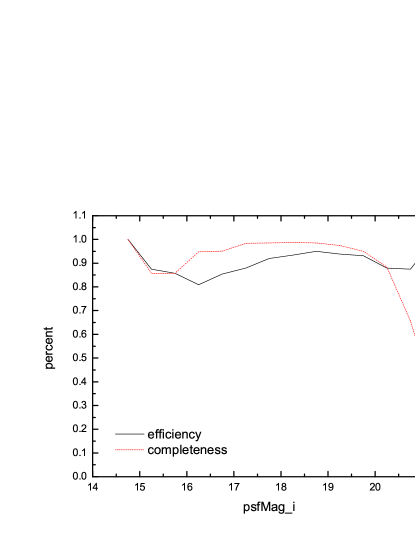
Figure 3: Efficiency and completeness as a function of magnitude $i$, solid line for efficiency, dotted line for completeness.

Until SDSS DR8 release, SDSS begins to provide a detailed subclasses of stars. The number of subclasses amounts to 43 considering each spectroscopically confirmed star. Table 4 shows that the number and the fraction of the 43 subclasses of stars are mixed into our predicted categories LowZ_QSO, MedZ_QSO and HighZ_QSO, respectively and provides what type of stars may mostly be mixed into quasars by SVM after Step_3. It is found that WD (45.95%), CV (33.49%), A0 (8.10%), CarbonWD (2.65%) and F5 (1.56%) can easily be misclassified as LowZ_QSO. Most of contaminants in MedZ_QSO are A0(27.27%), F5 (20.00%), G2 (10.91%), WD (10.91%) and F9 (9.09%). A0 and F5 stars can be easily misclassified into both low-redshift and medium-redshift quasars. The situation of HighZ_QSO is different that contaminants mainly come from K or M stars. The number in the parenthesis of Table 4 represents the misclassified stars before Step_3. We can find some information about Step_3 that SVM_30 can weed out some A0, CV and WD stars, SVM_31 mainly eliminate some A0 and F5 stars. Finally, the efficiency and the completeness of the SVM classification system is 93.21% and 97.49%, respectively. In Table 4, the final efficiency of these three subclasses is 90.62% (LowZ_QSO vs. other quasars and stars), 85.88% (MedZ_QSO vs. other quasars and stars) and 82.01% (HighZ_QSO vs. other quasars and stars) separately and the completeness of them is 97.35% (correctly predicted LowZ_QSO vs. all genuine LowZ_QSO), 74.35% (correctly predicted MedZ_QSO vs. all genuine MedZ_QSO) and 89.08% (correctly predicted HighZ_QSO vs. all genuine HighZ_QSO). For Carbon_lines, G5, L0, L1, L2, L3, L4, M0V, M2V, M5, M8, and M9 stars, none of them is misclassified into quasars. Figure 3 shows the efficiency and completeness as a function of magnitude $i$. However, the trend with magnitude $i<16.5$ is unreliable for the number of sample is just a few during this magnitude range. The real trend needs a larger sample to deduce. As magnitude $i>16.5$, the number of sample increases to hundreds or more than hundreds. Therefore the tendency in this range is credible. No matter for efficiency or completeness, the run is steady during the range $17<i<19.5$, then goes down beyond $i$=19.5. That the efficiency goes up and completeness declines beyond $i$=20.2 is unreliable due to small sample in this magnitude range and magnitude limit.

5 QUASAR CANDIDATE SELECTION

Through the above experiments, the SVM classification system proved applicable and reasonable to select quasar candidates from large sky survey projects. In order to further demonstrate the efficiency of this system, the comparison with the work of Bovy et al. (2011) has been done as follows. XD-sources is an unknown point-sources produced by Bovy et al. (2011) and we use it to generate a part of the quasar input catalog for Guoshoujing Telescope (LAMOST) with our SVM system in the pilot survey. SDSS-XDQSO quasar targeting catalog can be directly downloaded from the web page provided by Bovy et al. (2011). It includes 160,904,060 point-sources with dereddened $i$-band magnitude between 17.75 and 22.45 mag from SDSS DR8. The flag cuts for every source in this catalog have been used to filter unqualified ones. The detailed information about these flag cuts can be found in the Appendix A of the paper of Bovy et al. (2011). XDQSO technique has been applied on all objects in this catalog to provide the types and probabilities of them. Objects which satisfy the XDQSO probability cut P(XDQSO_MedZ)$>$0.424 will be selected as CORE targets in SDSS-III BOSS.

The Guoshoujing Telescope (LAMOST) is an innovative reflecting Schmidt telescope with 4 meter effective mirror size, 20 square degree field of view and 4000 fibres. It will perform most efficient optical spectroscopic sky survey. It entered the pilot survey phase in the end of 2011 and will carry out the regular survey in this year. Careful preparation of the input catalog for LAMOST is important for the scientific output of LAMOST. Since LAMOST has no own photometric data, the photometric data from other survey projects should be depended on, such as SDSS, UKIDSS, WISE, GALEX. In the pilot survey, two chunks are selected (-$45^{\circ}<\alpha_{\mathrm{J2000}}<+60^{\circ}$ and -$1^{\circ}.5<\delta_{\mathrm{J2000}}<+8^{\circ}.5$ ; $+180^{\circ}<\alpha_{\mathrm{J2000}}<+210^{\circ}$ and $+12^{\circ}<\delta_{\mathrm{J2000}}<+23^{\circ}$). We use the SVM classification system to select quasar candidates and compare our result with the targets selected by XDQSO technique in the both chunks.

Our SVM classification system obtains 64,660 targets in chunk1 and 29,520 targets in chunk2. Table 6 indicates that the selected quasar candidates by SVM overlap those by XDQSO in different probability ranges. Most of targets selected by SVM are covered by XDQSO especially for the highest probability ($P>0.99$) of XDQSO. In chunk1 and chunk2, 57.38% and 87.01% quasar candidates selected by SVM are also targeted by XDQSO. This can make the targets selected by SVM to a higher confidence. Table 7 indicates that the consistency of the two methods for classifying targets into three subcategories: low-redshift quasars, medium-redshift quasars and high-redshift quasars, and that the difference between the two methods is small except that some targets predicted as LowZ_QSO by SVM are classified by XDQSO as MedZ_QSO.

Actually, the amount of targets selected by this system is smaller than that by XDQSO because we want to get the higher predicted efficiency of quasars. In Figure 4, the predicted results of SVM in the two chunks as well as the overlaps of SVM and XDQSO are shown. It is found that the prediction of SVM coincides with that of XDQSO , especially in psfMag_i$<$20.0. The main reason of the difference of SVM and XDQSO in psfMag_i$>$20.0 maybe come from that the training sample includes so small a number of faint celestial objects that the ability of this system to recognize these objects is weak.

Table 6: The number per $deg^{2}$ of quasar candidates selected by SVM overlaps those selected by XDQSO in chunk1 and chunk2. The number in the parenthesis is produced by XDQSO.

XDQSO Probability	Chunk1 $deg^{2}$	Chunk2 $deg^{2}$
$0.990\leq P$	12.7 (15.9)	31.0 (40.0)
$0.950\leq P<0.990$	9.4 (12.6)	22.7 (31.3)
$0.900\leq P<0.950$	4.0 (7.3)	8.0 (16.9)
$0.850\leq P<0.900$	2.1 (5.2)	4.1 (12.1)
$0.800\leq P<0.850$	1.4 (4.7)	2.8 (10.9)
$0.750\leq P<0.800$	1.2 (4.4)	2.0 (10.6)
$0.700\leq P<0.750$	1.1 (4.5)	1.7 (10.6)
$0.650\leq P<0.700$	0.9 (4.7)	1.4 (10.6)
$0.600\leq P<0.650$	0.9 (5.0)	1.0 (10.6)
$0.550\leq P<0.600$	0.8 (5.3)	1.1 (11.6)
$0.500\leq P<0.550$	0.8 (5.9)	0.9 (11.7)

Table 7: The matrices of quasar candidates predicted as LowZ_QSO, MedZ_QSO and HighZ_QSO by SVM and XDQSO in chunk1 (No. 3,600,423 sources ) and chunk2 (No. 1,531,240 sources). Both the matrices reflect the agreement of the prediction of SVM and XDQSO.

Chunk1	SVM_LowZ	SVM_MedZ	SVM_HighZ
XDQSO_LowZ	30512	234	29
XDQSO_MedZ	997	4245	41
XDQSO_HighZ	8	14	1022
Chunk2	SVM_LowZ	SVM_MedZ	SVM_HighZ
XDQSO_LowZ	21022	122	6
XDQSO_MedZ	716	3004	13
XDQSO_HighZ	0	5	381

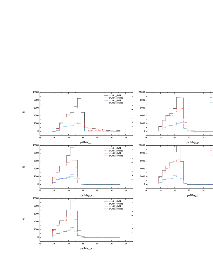
Figure 4: Comparison of the quasar candidates predicted only by SVM with those predicted both by SVM and XDQSO. The predictions of the two chunks are plotted separately. Chunk1_overlap and chunk2_overlap represent the quasar candidates selected both by SVM and XDQSO in these two pilot areas respectively. Solid line represents chunk1_SVM, long dashed line for chunk1_overlap, dotted line for chunk2_SVM, long dashed dotted line for chunk2_overlap.

6 CONCLUSIONS

We have put forward a classification system by using a hierarchy of several SVM classifiers. The above experimental results demonstrate that single SVM classifier can not well solve the problem of separating quasars from stars, however the combination of some SVM classifiers gets a rather good performance. This method can help us to select a quasar candidate set with a relative high efficiency (93.21%), though some actual quasars (2.51%) are missing in the whole process. The point we want to get across is that the performance of this system is based on the test sample and not on real data. In order to check the performance of this method applied on the unknown objects, the result produced by the method has been compared with that of the XDQSO technique. The comparison shows that most of quasar candidates selected by the SVM system are also recovered by XDQSO especially in the deredened i-band magnitude $<$ 20.0. In Table 7, actually the prediction of SVM for subclasses of quasars also agrees with that of XDQSO. This means that our method is an effective and feasible approach to construct the input catalog of quasars for large spectroscopic sky survey projects (e.g. LAMOST, SDSS ).

In the future, we plan to adopt the similar method to the XDQSO technique to exploit whether the magnitude errors influence the performance of the system, add the number of faint objects in the training sample increases to improve the performance of the system for the data set of faint objects (deredened i-band magnitude $>$ 20.0). In the process of SVM_1 where many actual quasars are missing, we can consider some other methods to make the completeness of quasars much higher. Each technique for quasar candidate selection has its strongness and weakness. It is difficult to say which one is better. In terms of good efficiency, the cross-result from different techniques to select quasar candidates is better chosen. However, given the completeness of quasar candidates, the combination of results from various techniques has better be employed. We will give a much more powerful method based on SVM to select quasar candidates for LAMOST or other projects in the world.

Appendix A THE MODEL PARAMETERS OF SVM

Model parameters of SVM can greatly affect the performance of SVM for selecting quasar candidates. We generate SVM models using the following model parameters.

$$\begin{array}[]{rrllll}{\rm A})&SVM\_0&t=2&c=100&j=1&g=1\\ {\rm B})&SVM\_1&t=2&c=0.07&j=1&g=1\\ {\rm C})&SVM\_20&t=2&c=0.2&j=1&g=1\\ {\rm D})&SVM\_21&t=2&c=0.25&j=1&g=1\\ {\rm E})&SVM\_22&t=2&c=6&j=1&g=1\\ {\rm F})&SVM\_23&t=2&c=0.04&j=1&g=1\\ {\rm F})&SVM\_24&t=2&c=29&j=1&g=1\\ {\rm F})&SVM\_25&t=2&c=0.16&j=1&g=1\\ {\rm F})&SVM\_30&t=2&c=0.12&j=1&g=1\\ {\rm F})&SVM\_31&t=2&c=0.06&j=1&g=1\\ {\rm G})&SVM\_32&t=2&c=0.5&j=1&g=1\end{array}$$ (19)

The parameter $t=2$ represents that SVM uses radial basis function (RBF) kernel for deriving models. The parameter $c$ controls the trade-off between training error and margin. The parameter $j$ in a SVM model dominates the misclassification cost of quasars or stars. The parameter $g$ means $\gamma$ in RBF kernel. In this work, we just use the default value of $g$ which is equal to 1. The more detailed information about how these parameters affect the performance of SVM can be found in Joachims (2002). In order to search the optimal combination of parameters $c$ and $j$, we usually test each pair of parameters appeared in the specified sequence which is determined by experience. For example, the first model (SVM_0) of this system, the parameters $c$ and $j$ are from the values [0.2, 0.5, 1, 2, 5, 10, 20, 50, 100]. The above mentioned parameters for each SVM model are produced by an empirical approach because the computing time to search the optimal parameters $c$ and $j$ is expensive. At the beginning, we just set the parameters $j$ and $g$ with default value 1. The value of parameter $c$ can be calculated by using the sample size of stars divided by that of quasars. This empirical method can help us to quickly get a better parameter combination.

References

- [Abazajian et al. 2009] Abazajian K.N. et al., 2009, ApJS, 182, 543
- [Abraham et al. 2010] Abraham S., Sajeeth Philip N., Kembhavi A., Wadadekar Y. G., Sinha R., 2010, eprint arXiv:1011.2173
- [Aihara H. et al. 2011] Aihara H. et al., 2011, ApJS, 193, 29
- [Bailer-Jones C.A.L. et al. 2008] Bailer-Jones C.A.L., Smith K.W., Tiede C., Sordo R., Vallenari A., 2008, MNRAS, 391, 1838
- [Ball N. M. & Brunner R. J. 2010] Ball N. M. & Brunner R. J. 2010, IJMPD, 19, 1049
- [Borne 2009] Borne K., 2002, eprint arXiv:0911.0505
- [Bovy et al. 2011] Bovy J. et al., 2011, ApJ, 729, 141
- [Burges, C.J.C. 1998] Burges, C.J.C., 1998, PR, 167, 161
- [Carballo et al. 2008] Carballo R., González-Serrano J. I., Benn C. R., Jiménez-Luján F., 2008, MNRAS, 391, 369
- [D’Abrusco R., Longo G., Walton N.A. 2009] D’Abrusco R., Longo G., Walton N.A., 2009, MNRAS, 396, 223
- [Meyer D. 2001] Meyer D., 2001, R News, 23, 1(3)
- [Eisenstein D.J. et al. 2011] Eisenstein D.J. et al., 2011, eprint arXiv:1101.1529
- [Gao D., Zhang Y.-X., Zhao Y.-H. 2008] Gao D., Zhang Y.-X., Zhao Y.-H., 2008, MNRAS, 386, 1417
- [Joachims T. 2002] Joachims T. 2002, Learning to Classify Text Using Support Vector Machines, Kluwer Academic Publishers, MA
- [Kaiser & Aussel 2002] Kaiser N. & Aussel H., 2002, SPIE, 4836, 154
- [Kim D.-W. et al. 2011] Kim D.-W., Protopapas P., Alcock C., Byun Y.-I., Khardon R., 2011, ASPC, 442, 447
- [Kirtpatrik J.A. et al. 2011] Kirtpatrik J.A. et al., 2011, eprint arXiv:1104.4995
- [Lawrence A. et al. 2007] Lawrence A. et al., 2007, MNRAS, 379, 1599
- [McPherson et al. 2006] McPherson A.M. et al., 2006, SPIE, 6267
- [Morik K., Brockhausen P., Joachims T. 1999] Morik K., Brockhausen P., Joachims T., 1999, ML, CONF 16, 268
- [Richards G.T. et al. 2002] Richards G.T. et al. 2002, AJ, 123, 2945
- [Richards G.T. et al. 2004] Richards G.T. et al. 2004, ApJS, 155, 257
- [Richards G.T. et al. 2009] Richards G.T. et al. 2009, ApJS, 180, 67
- [Ross N.P. et al. 2011] Ross N.P. et al. 2011, eprint arXiv:1105.0606
- [Schlegel D.J. et al. 1998] Schlegel D.J., Finkbeiner D. P., Davis M., 1998, ApJ, 500, 525
- [Schlegel D.J. et al. 2007] Schlegel D.J. et al. 2007, BAAS, 38, 996
- [Schneider D.P. et al. 2010] Schneider D.P. et al. 2010, AJ, 139, 2360
- [Tyson 2002] Tyson J.A., 2002, SPIE, 4836, 10
- [Vapnik V.N. 1995] Vapnik V.N. 1995, The nature of statistical learning theory, Springer US, NY
- [Vapnik V.N. 1998] Vapnik V.N. 1998, Statistical Learning Theory, John Wiley and Sons, NY
- [Wu X.-B. & Jia Z.-D. 2010] Wu X.-B. & Jia Z.-D., 2010, MNRAS, 406, 1583
- [Wu X.-B. et.al. 2011] Wu X.-B., Wang R., Schmidt K. B., Bian F., Jiang L., Fan X., 2011, MNRAS, 142, 78
- [Yéche C. et al. 2010] Yéche C. et al. 2010, A&A, 523, A14
- [York, et al,] York, D. G., et al., 2000, AJ, 120, 1579
- [Zhang Y.-X. & Zhao Y.-H. 2003] Zhang Y.-X., & Zhao Y.-H., 2003, PASP, 115, 1006
- [Zhang Y.-X. & Zhao Y.-H. 2004] Zhang Y.-X., & Zhao Y.-H., 2004, A&A, 422, 1113