Constrained energy minimization
and
ground states for NLS with point defects

Abstract.

We investigate the ground states of the one-dimensional nonlinear Schrödinger equation with a defect located at a fixed point. The nonlinearity is focusing and consists of a subcritical power. The notion of ground state can be defined in several (often non-equivalent) ways. We define a ground state as a minimizer of the energy functional among the functions endowed with the same mass. This is the physically meaningful definition in the main fields of application of NLS. In this context we prove an abstract theorem that revisits the concentration-compactness method and which is suitable to treat NLS with inhomogeneities. Then we apply it to three models, describing three different kinds of defect: delta potential, delta prime interaction, and dipole. In the three cases we explicitly compute ground states and we show their orbital stability. This problem had been already considered for the delta and for the delta prime defect with a different constrained minimization problem, i.e. defining ground states as the minimizers of the action on the Nehari manifold. The case of dipole defect is entirely new.

1. Introduction

Several one-dimensional physical systems are driven by the focusing nonlinear Schrödinger equation (NLS)

$$i\partial_{t}v+Hv=v|v|^{p-1},\quad 1<p<5,\quad v:(t,x)\mapsto v(t,x)\in{\mathbb{C}},\quad v(t,\cdot)\in L^{2}({\mathbb{R}}),$$ (1.1)

where $H$ is a selfadjoint operator on $L^{2}({\mathbb{R}})$. A first fundamental step in studying the dynamics of this system concerns the possible existence and properties of standing waves and, among them, of the ground states. While the former are defined as stationary solutions to equation (1.1), the latter are characterized in terms of variational properties. Generalizing the usual notion of ground state in linear quantum mechanics to nonlinear systems, one is led to introduce ground states as the minimizers of the energy among the functions endowed with the same $L^{2}$-norm. Indeed, out of the realm of linear quantum mechanics, such a notion still proves meaningful, as the $L^{2}$-norm often represents some physically relevant quantities, e.g. number of particles in Bose-Einstein condensates, or power supply in nonlinear optics propagation, which are two main fields of application of NLS. While the definition above is common not only in the physical but also in the mathematical literature, for example in the classical analysis based on concentration-compactness methods (see [15, 16] and references therein), in most recent papers dealing with NLS with inhomogeneities and defects (see e.g. [22, 23, 31, 4]) it is preferred to define as ground states the minimizers of the so-called action functional among the functions belonging to the natural Nehari manifold associated to the functional. Such a notion corresponds to a different way of controlling the physical system, and mathematically often proves easier to handle. In the present paper we adopt the former definition and after proving a general theorem for the ground states of (1.1), we apply it to NLS with point inhomogeneities of various types to show existence and orbital stability of the ground states. Moreover, we give the explicit expression of the family of the ground states in the considered examples. The common characteristic in these applications is the lack of symmetry with respect to the standard NLS due to the presence of a defect in the propagating medium. Such a feature has relevant consequences on the family of stationary states: when the operator $H$ is the one-dimensional laplacian, equation (1.1) is invariant under the action of the Galileo group, and this symmetry leads to a rich family of solitary waves, consisting of orbits of the existing symmetries. We are interested in situations in which some symmetries are possibly broken by the operator $H$, but some of them survive and give rise to standing waves. More specifically, in the examples treated in Sections 2, 4, 5, 6, translational symmetry is lost due to singularities in the elements of the domain of $H$, but $U(1)$-symmetry is preserved.

To cast the issue in a suitable generality we pose, in the same spirit (but in a different situation) of [10], the following family of variational problems

$$I(\rho)\ :=\ \inf_{\begin{subarray}{c}u\in{\mathcal{H}}\\ \|u\|_{L^{2}({\mathbb{R}})}=\rho\end{subarray}}{\mathcal{E}}(u)$$ (1.2)

where

$${\mathcal{E}}(u)=\frac{1}{2}Q(u,u)-\frac{1}{p+1}\|u\|_{L^{p+1}({\mathbb{R}})}^{p+1}$$

is the energy associated to equation (1.1), whose value is conserved by the flow, and

$$Q:{\mathcal{H}}\times{\mathcal{H}}\rightarrow{\mathbb{R}}$$

is a non-negative quadratic form on a Hilbert space ${\mathcal{H}}$. Of course, for a concrete dynamics like (1.1), the space ${\mathcal{H}}$ does not coincide with $L^{2}({\mathbb{R}})$, but rather with the domain of the quadratic form associated to the operator $H$, which is smaller than $L^{2}({\mathbb{R}})$.

To the aim of proving our abstract results, the Hilbert space ${\mathcal{H}}$ is required to have an embedding in $L^{2}({\mathbb{R}})\cap L^{p+1}({\mathbb{R}})$ in which the validity of Gagliardo-Nirenberg type inequalities is assumed, as well as a.e. pointwise convergence (up to subsequences) of weakly convergent sequences in ${\mathcal{H}}$. The quadratic form must have a splitting property (see (2.4)) and a continuity property (see (2.5)) with respect to weak convergence. With these hypotheses, in Theorem 2.1 we prove a variant of the concentration-compactness method according to which, if non-vanishing of minimizing sequence $u_{n}$ is guaranteed from the outset, then $u_{n}$ is compact in $\mathcal{H}$.

The connection of this abstract framework with the equation (1.1) is easily established: given the embedding of ${\mathcal{H}}$ in $L^{2}({\mathbb{R}})$, and provided that $Q$ is closed and semibounded, then $Q$ is associated to a unique selfadjoint operator $H$, and by Lagrange multiplier theorem and standard operator theory, the minimizers of (1.2) must solve the stationary equation

$$Hu\ -\ u|u|^{p-1}=-\omega u$$ (1.3)

where $\omega$ is a Lagrange multiplier. As in the case of the free laplacian, for a more general $H$ solutions to (1.3) exist in $L^{2}({\mathbb{R}})$ only for $\omega$ in a suitable range, giving rise to a branch of stationary solutions; moreover, the corresponding function $v(x,t)=e^{-i\omega t}u(x)$ is a standing wave solution to (1.1). This standing wave, being a solution of the minimum problem (1.2), is a ground state, and, thanks to a classical argument (see [15, 16]), is moreover orbitally stable.

Our main concern in the application of this abstract result is the case in which the quadratic form $Q$ describes a so-called point interaction ([8, 7]), that is a singular perturbation at a point of the one-dimensional laplacian.

A summary of the basic definitions and of the main results on point interactions is provided in Section 7. Here, for the convenience of the reader, we limit to a general description. Let us consider the closed symmetric laplacian on the domain $C^{\infty}_{0}({\mathbb{R}}\setminus\{0\})$. On such a domain the laplacian has deficiency indices $(2,2)$ and owing to the Von Neumann-Krein theory it has a four-parameter family of selfadjoint extensions, called point interactions. The elements in the domain of these operators are characterized by suitable bilateral boundary conditions at the singularity (see formula (7.2)), while the action coincides with the laplacian out of the singularity. The most popular point interaction is the $\delta$ interaction, more often called in the physical literature $\delta$ potential or $\delta$ defect, defined by the well-known boundary conditions (7.4).

We interpret, quite generally, singular perturbations $H$ of the one-dimensional laplacian as describing models of strongly localized, ideally pointlike, defect or inhomogeneity in the bulk of the medium in which NLS propagation occurs. The interactions between field and defect are of importance in the study of one-dimensional evolution of Bose-Einstein (“cigar-shaped”) condensates or the propagation of laser pulses in a nonlinear Kerr medium. In the physical literature, standing waves of NLS with a defect are often considered for the relevant cubic case ($p=3$) and in this context they are called defect or pinned modes. They are studied, to the knowledge of the authors, in the special model case of $\delta$ potential only (see [14, 36, 5] and references therein).

It is an interesting fact that, beside this analytical and numerical work, recently has been experimentally demonstrated the relevant physical phenomenon of trapping of optical solitons in correspondence of a defect (a localized photonic potential), present (or put) in the nonlinear medium ([32]).

Rigorous studies of NLS in the presence of impurities described by point interactions have been given along several lines, still with an almost exclusive treatment of $\delta$ potential. The focus of the currently active mathematical research is on orbital stability of standing waves for subcritical NLS with a $\delta$ potential ([23, 22, 31, 2]) and $\delta^{\prime}$ interaction ([4]), scattering properties of asymptotically solitary solutions of cubic NLS with a $\delta$ potential ([29, 18]) with generalization to the case of star graphs ([1]), and breathing in nonlinear relaxation ([30]); finally, a thorough analysis by means of inverse scattering methods for a cubic NLS with $\delta$ potential and even initial data, with results on asymptotic stability of solutions, is given in [19]. Concerning more general issues, in [3] the well-posedness of the dynamics is proved for the whole family of point interactions in the cubic case. More relevant to the issue of the present paper is the content of [26], where a variational characterization of standing waves of NLS with a $\delta$ potential which is similar to ours in spirit is stated without proof. Here we treat in detail the case of $\delta$ potential, filling the gap in [26], and also the more singular cases of $\delta^{\prime}$ interaction and dipole interaction. At variance with the $\delta$ defect, whose form domain coincides with the Sobolev space $H^{1}({\mathbb{R}})$, the latter have a form domain given by $H^{1}({\mathbb{R}}^{-})\oplus H^{1}({\mathbb{R}}^{+})$, and boundary conditions in the operator domain which allow for discontinuities of the elements of the domain at the position of the defect ($\delta^{\prime}$ interaction, see (7.5)) or in both the element of the domain and its derivative (dipole interaction, see (7.6)). In particular, concerning this last example, we stress the fact that only very recently it has been recognized that dipole interaction represents the singular perturbation of the laplacian which correctly describes a $\delta^{\prime}$ potential, i.e. the derivative of a $\delta$, in the sense that it can be approximated by suitable rescaled potentials which converge in distributional sense to a $\delta^{\prime}$ distribution (see [25], [37], [38] and the Appendix I for a brief discussion).

We start with the case of the $\delta$ potential, described by Corollary 2.1, and, for $1<p<5$ and for every positive fixed mass, we prove minimization of the energy functional and we explicitly give the set of the minima and the related orbital stability. The same result holds true for the critical case $p=5$ if the mass is small enough, however we skip the treatment of this case in order to shorten the presentation. We emphasize again that, also in the case of $\delta$ potential, in which the variational setting is milder, the standing waves and their stability properties were known, but their present characterization through constrained energy minimization was not. In particular, the cited papers [23, 22, 31] treated orbital stability through the method due to Weinstein and Grillakis-Shatah-Strauss, i.e. constrained linearization ([34, 35, 27, 28]). Corollaries 2.2 and 2.3 give the minimization properties and, correspondingly, orbital stability of the set of minima for the $\delta^{\prime}$ interaction and dipole interaction, for which nothing (except the results in [4]) had been previously studied in the literature. The results are analogous to those known for the $\delta$ case, even if the statements and the proofs are more difficult due to the more complicated structure of the set of minima, which presents a spontaneous symmetry breaking, and to the presence of a singularity in the elements of the energy domain. The last treated case is the dipole interaction, for which we give the explicit set of standing waves, that splits in two subfamilies, one composed of orbitally stable ground states, and the other of excited states. This case is entirely new.

The plan of the paper is the following. In Section 2, after a preliminary presentation of the variational framework, the statement of the main general Theorem 2.1 is given and the applications to point interactions are stated. In Section 3 the main theorem is proved, while the proof of the results on variational characterization of ground states for NLS with point interactions are given in Sections 4, 5 and 6. Two appendices close the paper. Appendix I provides a short review of the theory of point interactions on the line, including those not widely known, and of the main properties of their quadratic forms. In Appendix II we present, making use of an elementary analysis of the Cauchy problem for the stationary NLS with power nonlinearity on the halfline, the explicit structure of standing waves for NLS with point defects. Other cases of point interactions can be treated with the same general method.

2. An Abstract Result and Applications to NLS with Point Interaction

The variational problems we are interested in share the following variational structure:

$$I(\rho)\ :=\ \inf_{\begin{subarray}{c}u\in{\mathcal{H}}\\ \|u\|_{L^{2}({\mathbb{R}})}=\rho\end{subarray}}{\mathcal{E}}(u)$$ (2.1)

where

$${\mathcal{E}}(u)=\frac{1}{2}Q(u,u)-\frac{1}{p+1}\|u\|_{L^{p+1}({\mathbb{R}})}^{p+1}$$

and

$$Q:{\mathcal{H}}\times{\mathcal{H}}\rightarrow{\mathbb{R}}$$

is a non-negative quadratic form on a Hilbert space ${\mathcal{H}}\ .$

On the Hilbert space ${\mathcal{H}}$ we assume the following properties:

$${\mathcal{H}}\subset L^{2}({\mathbb{R}})\cap L^{p+1}({\mathbb{R}})$$ (2.2)

$$\hbox{ and }\exists\hbox{ }C>0,\sigma\in(0,1)\hbox{ s.t. }\|u\|_{L^{p+1}({\mathbb{R}})}\leq C\|u\|_{L^{2}({\mathbb{R}})}^{\sigma}\|u\|_{\mathcal{H}}^{1-\sigma};$$

$$\hbox{ if }u_{n}\rightharpoonup\bar{u}\hbox{ in $\mathcal{H}$, then up to subsequences }u_{n}(x)\rightarrow\bar{u}(x)\hbox{ a.e. }x\in{\mathbb{R}}$$ (2.3)

Example 2.1.

In the following sections we deal with three examples of Hilbert spaces satisfying the previous requirements: they are given by $H^{1}({\mathbb{R}})$ (associated to the $\delta$ potential), $H^{1}({\mathbb{R}}^{-})\oplus H^{1}({\mathbb{R}}^{+})$ (associated to the $\delta^{\prime}$ interaction), and $H_{\tau}=\{\psi\in H^{1}({\mathbb{R}}^{-})\oplus H^{1}({\mathbb{R}}^{+}),\psi(0+)=\tau\psi(0-)\}$ (associated to the dipole interaction or $\delta^{\prime}$ potential).

Concerning the quadratic form $Q(.,.)$, the following assumptions are made:

$$u_{n}\rightharpoonup\bar{u}\hbox{ in $\mathcal{H}$ }\Longrightarrow Q(u_{n}-\bar{u},u_{n}-\bar{u})=Q(u_{n},u_{n})-Q(\bar{u},\bar{u})+o(1);$$ (2.4)

$$u_{n}\rightharpoonup\bar{u}\hbox{ in $\mathcal{H}$ and }Q(u_{n},u_{n})=Q(\bar{u},\bar{u})+o(1)\Longrightarrow u_{n}\rightarrow\bar{u}\hbox{ in }\mathcal{H}$$ (2.5)

Example 2.2.

Every continuous quadratic form satisfies (2.4). Concerning (2.5), it is satisfied by any quadratic form with the following structure:

$$Q(u,u)=\|u\|_{\mathcal{H}}^{2}+K(u,u)$$

where $K:{\mathcal{H}}\times{\mathcal{H}}\rightarrow{\mathbb{R}}$ is such that:

$$u_{n}\rightharpoonup\bar{u}\hbox{ in $\mathcal{H}$ }\Longrightarrow K(u_{n},u_{n})\rightarrow K(\bar{u},\bar{u})$$

Next we state a general result on the compactness of minimizing sequences to the minimization problems (1.2) under suitable assumptions on the form $Q(.,.)$.

Theorem 2.1.

Let $Q$ be a non-negative quadratic form on the Hilbert space $\mathcal{H}$ and assume (2.2), (2.3), (2.4), (2.5). Let $u_{n}\in\mathcal{H}$ be a minimizing sequence for $I(\rho)$, i.e.

$$\|u_{n}\|_{L^{2}({\mathbb{R}})}=\rho\hbox{ and }\lim_{n\rightarrow\infty}{\mathcal{E}}(u_{n})=I(\rho).$$

Assume moreover that:

$$u_{n}\rightharpoonup\bar{u}\neq 0\hbox{ in }\mathcal{H};$$ (2.6)

$$I(\mu)<0,\hbox{ }\forall\hbox{ }0<\mu\leq\rho;$$ (2.7)

for any compact set $$K\subset(0,\rho]$$ we have (2.8)

$$\sup_{\begin{subarray}{c}\{u\in{\mathcal{H}}|{\mathcal{E}}(u)<0\\ \|u\|_{L^{2}({\mathbb{R}})}=\mu,\mu\in K\}\end{subarray}}\|u\|_{\mathcal{H}}<\infty$$

Then $u_{n}\rightarrow\bar{u}\hbox{ in }\mathcal{H}$ and in particular $\bar{u}$ is a minimizer for (1.2).

We give some applications of the previous general theorem to deduce the existence and the stability of standing waves for NLS with singular perturbation of the laplacian described by point interactions.

1. We begin with the so-called attractive $\delta$ interaction. In our notation the pertinent NLS is

$$i\partial_{t}v+H_{\alpha}^{\delta}v=v|v|^{p-1},$$ (2.9)

where $H_{\alpha}^{\delta}$ is the operator on $L^{2}({\mathbb{R}})$ defined on the domain

$$D(H_{\alpha}^{\delta})\ :=\ \left\{u\in H^{2}({\mathbb{R}}\backslash\{0\}),\ u(0+)=u(0-),\ u^{\prime}(0+)-u^{\prime}(0-)=-\alpha u(0+),\ \alpha>0\right\},$$

and its action reads

$$(H_{\alpha}^{\delta}u)(x)\ =\ -u^{\prime\prime}(x),\qquad x\neq 0.$$

The parameter $\alpha$ is interpreted as the strength of the $\delta$ potential (see also Appendix I).

In order to deduce the existence and stability of standing waves to (2.9), according to a general argument introduced in [16] it is sufficient to prove the compactness of minimizing sequences to the following variational problems:

$$I^{{\mathcal{E}}_{\alpha,p}^{\delta}}(\rho)\ :=\ \inf_{\begin{subarray}{c}u\in H^{1}({\mathbb{R}})\\ \|u\|_{L^{2}({\mathbb{R}})}=\rho\end{subarray}}{\mathcal{E}}_{\alpha,p}^{\delta}$$

where

$${\mathcal{E}}_{\alpha,p}^{\delta}(u)=\frac{1}{2}\|u^{\prime}\|_{L^{2}({\mathbb{R}})}^{2}-\frac{\alpha}{2}|u(0)|^{2}-\frac{1}{p+1}\|u\|_{L^{p+1}({\mathbb{R}})}^{p+1}$$

is the energy associated to (2.9).

We also denote by ${\mathcal{M}}^{{\mathcal{E}}_{\alpha,p}^{\delta}}(\rho)$ the corresponding set of minimizers (provided that they exist).
To present our next result we introduce the function

$$u_{\alpha,p,\omega}(x)\ :=\ \left(\frac{\omega(p+1)}{2\cosh^{2}(\frac{p-1}{2}\sqrt{\omega}(|x|+\tilde{x}))}\right)^{\frac{1}{p-1}}$$ (2.10)

where $\tilde{x}=\tilde{x}(\alpha,\omega,p)$ is given by

$$\tanh\left(\frac{p-1}{2}\sqrt{\omega}\tilde{x}\right)=\frac{\alpha}{2\sqrt{\omega}},$$ (2.11)

and the map

$$h_{\alpha,p}:(\alpha^{2}/4,\infty)\ni\omega\mapsto\|u_{\alpha,p,\omega}\|_{L^{2}({\mathbb{R}})}\in(0,\infty)\ .$$

In Corollary 8.1 we prove by elementary computation that $h_{\alpha,p}$ is a monotonically increasing bijection (see also [23]), and in particular it is well defined its inverse function

$$g_{\alpha,p}:(0,\infty)\rightarrow(\alpha^{2}/4,\infty).$$

Corollary 2.1.

Let $\alpha>0$, $1<p<5$ and $\rho>0$ be fixed. Let $u_{n}\in H^{1}({\mathbb{R}})$ be a minimizing sequence for $I^{{\mathcal{E}}_{\alpha,p}^{\delta}}(\rho)$, i.e.

$$\|u_{n}\|_{L^{2}({\mathbb{R}})}=\rho\hbox{ and }\lim_{n\rightarrow\infty}{\mathcal{E}}_{\alpha,p}^{\delta}(u_{n})=I^{{\mathcal{E}}_{\alpha,p}^{\delta}}(\rho)$$

Then

• a) the sequence $u_{n}$ is compact in $H^{1}({\mathbb{R}})$;

• b) the set of minima is given by

  $${\mathcal{M}}^{{\mathcal{E}}_{\alpha,p}^{\delta}}(\rho)=\left\{e^{i\gamma}u_{\alpha,p,g_{\alpha,p}(\rho)},\forall\gamma\in{\mathbb{R}}\right\};$$

• c) for every $\rho>0$ the set ${\mathcal{M}}^{{\mathcal{E}}_{\alpha,p}^{\delta}}(\rho)$ is orbitally stable under the flow associated to (2.9).

2. An analogous result holds true for the case of a nonlinear Schrödinger equation with an attractive $\delta^{\prime}$ interaction (see Appendix I) described by the equation

$$i\partial_{t}v+H_{\beta}^{\delta^{\prime}}v=v|v|^{p-1},$$ (2.12)

where the operator $H_{\beta}^{\delta^{\prime}}$ is defined by

$$\begin{split}D(H_{\beta}^{\delta^{\prime}})&\ :=\ \left\{u\in H^{2}({\mathbb{R}}\backslash\{0\}),\ u^{\prime}(0+)=u^{\prime}(0-),\ u(0+)-u(0-)=-\beta u^{\prime}(0+),\ \beta>0\right\},\\ H_{\beta}^{\delta^{\prime}}u(x)&\ =\ -u^{\prime\prime}(x),\qquad x\neq 0.\end{split}$$

The operator $H_{\beta}^{\delta^{\prime}}$ is selfadjoint on $L^{2}({\mathbb{R}})$.

In analogy with the case of the $\delta$ interaction, we are interested in the associated minimization problem:

$$I^{{\mathcal{E}}_{\beta,p}^{\delta^{\prime}}}(\rho)\ :=\ \inf_{\begin{subarray}{c}u\in H^{1}({\mathbb{R}}^{-})\oplus H^{1}({\mathbb{R}}^{+})\\ \|u\|_{L^{2}({\mathbb{R}})}=\rho\end{subarray}}{\mathcal{E}}_{\beta,p}^{\delta^{\prime}}$$ (2.13)

where

$${\mathcal{E}}_{\beta,p}^{\delta^{\prime}}(u)=\frac{1}{2}\left(\|u^{\prime}\|_{L^{2}({\mathbb{R}}^{-})}^{2}+\|u^{\prime}\|_{L^{2}({\mathbb{R}}^{+})}^{2}\right)-\frac{1}{2\beta}|u(0+)-u(0-)|^{2}-\frac{1}{p+1}\|u\|_{L^{p+1}({\mathbb{R}})}^{p+1}.$$

We stress that in the previous definition, we denoted

$$\|u^{\prime}\|_{L^{2}({\mathbb{R}}^{-})}^{2}+\|u^{\prime}\|_{L^{2}({\mathbb{R}}^{+})}^{2}\ =\ \lim_{\varepsilon\to 0+}\left(\int_{-\infty}^{-\varepsilon}|u^{\prime}(x)|\,dx+\int^{\infty}_{\varepsilon}|u^{\prime}(x)|\,dx\right).$$

Besides, notice that $u(0\pm)$ are well defined due to well-known continuity property of functions belonging to $H^{1}({\mathbb{R}}^{-})\oplus H^{1}({\mathbb{R}}^{+})$.

We also denote by ${\mathcal{M}}^{{\mathcal{E}}_{\beta,p}^{\delta^{\prime}}}(\rho)$ the corresponding set of minimizers.

Next, to explicitly describe minimizers, we introduce two families of functions; the members of the first family are odd on ${\mathbb{R}}$ and the members of the second family do not enjoy any symmetry, so we call them asymmetric. Explicitly (see Propositions 8.4 and 8.5),

$$u_{odd,\beta,p,\omega}(x)=\left(\frac{\omega(p+1)}{2\cosh^{2}(\frac{p-1}{2}\sqrt{\omega}(|x|+\bar{x}))}\right)^{\frac{1}{p-1}}\hbox{ for }x\in{\mathbb{R}}$$

where $\beta\sqrt{\omega}\tanh\left(\frac{p-1}{2}\sqrt{\omega}\bar{x}\right)=2,$ so $\bar{x}>0;$

$$u_{as,\beta,p,\omega}(x)=\pm\left(\frac{\omega(p+1)}{2\cosh^{2}(\frac{p-1}{2}\sqrt{\omega}(x+x_{\pm}))}\right)^{\frac{1}{p-1}}\ \hbox{ for }x\in{\mathbb{R}}^{\pm}.$$

where, for $\omega>\frac{4}{\beta^{2}}\frac{p+1}{p-1}$, the couple $(x_{+},x_{-})$ is the only solution to the transcendental system (8.9) with $x_{-}<0<x_{+}<|x_{-}|$.

We need also to define the map

$$h_{\beta,p}:(4/\beta^{2},\infty)\rightarrow(0,\infty)$$

such that

$$h_{\beta,p}(\omega)=\left\{\begin{array}[]{ll}\|u_{odd,\beta,p,\omega}\|_{L^{2}({\mathbb{R}})}&\hbox{ for }\omega\in(\frac{4}{\beta^{2}},\frac{4}{\beta^{2}}\frac{p+1}{p-1}]\\ \|u_{as,\beta,p,\omega}\|_{L^{2}({\mathbb{R}})}&\hbox{ for }\omega\in(\frac{4}{\beta^{2}}\frac{p+1}{p-1},\infty)\end{array}\right.$$

By Proposition 8.6 the function $h_{\beta,p}$ is continuous, monotonically increasing and surjective, hence there exists its inverse function

$$g_{\beta,p}:(0,\infty)\rightarrow(4/\beta^{2},\infty)$$

Now we can give the statement of the Corollary that embodies the applications of Theorem 2.1 to the problem (2.13).

Corollary 2.2.

Let $\beta>0$, $1<p<5$ and $\rho>0$ be fixed. Let $u_{n}\in H^{1}({\mathbb{R}}^{-})\oplus H^{1}({\mathbb{R}}^{+})$ be a minimizing sequence for $I^{{\mathcal{E}}_{\beta,p}^{\delta^{\prime}}}(\rho)$, i.e.

$$\|u_{n}\|_{L^{2}({\mathbb{R}})}=\rho\hbox{ and }\lim_{n\rightarrow\infty}{\mathcal{E}}_{\beta,p}^{\delta^{\prime}}(u_{n})=I^{{\mathcal{E}}_{\beta,p}^{\delta^{\prime}}}(\rho)$$

Then,

• a) the sequence $u_{n}$ is compact in $H^{1}({\mathbb{R}}^{-})\oplus H^{1}({\mathbb{R}}^{+})$;

• b) the set of minima is given by:

  $${\mathcal{M}}^{{\mathcal{E}}_{\beta,p}^{\delta^{\prime}}}(\rho)=\left\{e^{i\gamma}u_{odd,\beta,p,g_{\beta,p}(\rho)},\forall\gamma\in{\mathbb{R}}\right\}\hbox{ if }g_{\beta,p}(\rho)\in\left(\frac{4}{\beta^{2}},\frac{4}{\beta^{2}}\frac{p+1}{p-1}\right];$$

  $${\mathcal{M}}^{{\mathcal{E}}_{\beta,p}^{\delta^{\prime}}}(\rho)=\left\{e^{i\gamma}u_{as,\beta,p,g_{\beta,p}(\rho)}(\pm\cdot),\forall\gamma\in{\mathbb{R}}\right\}\hbox{ if }g_{\beta,p}(\rho)\in\left(\frac{4}{\beta^{2}}\frac{p+1}{p-1},\infty\right);$$

• c) for every $\rho>0$ the set ${\mathcal{M}}^{{\mathcal{E}}_{\beta,p}^{\delta^{\prime}}}(\rho)$ is orbitally stable under the flow associated to (2.12).

3. As a last example, we study the nonlinear Schrödinger equation with a dipole interaction

$$i\partial_{t}v+H_{\tau}^{dip}v=v|v|^{p-1},$$ (2.14)

where $H_{\tau}^{dip}$ is the operator defined on the domain

$$D(H_{\tau}^{dip})\ :=\ \{u\in H^{2}({\mathbb{R}}\backslash\{0\}),\ u(0+)=\tau u(0-),\ u^{\prime}(0-)=\tau u^{\prime}(0+)\}.$$

In analogy with the previous point interactions we are interested in the following variational problem:

$$I_{\tau}^{{\mathcal{E}}_{p}^{dip}}(\rho)\ :=\ \inf_{\begin{subarray}{c}u\in{\mathcal{H}}^{\tau}\\ \|u\|_{L^{2}({\mathbb{R}})}=\rho\end{subarray}}{\mathcal{E}}_{p}^{dip}$$

where

$${\mathcal{E}}_{p}^{dip}(u)=\frac{1}{2}\left(\|u^{\prime}\|_{L^{2}({\mathbb{R}}^{-})}^{2}+\|u^{\prime}\|_{L^{2}({\mathbb{R}}^{+})}^{2}\right)-\frac{1}{p+1}\|u\|_{L^{p+1}({\mathbb{R}})}^{p+1},$$

and

$${\mathcal{H}}^{\tau}=\{u\in H^{1}({\mathbb{R}}^{-})\oplus H^{1}({\mathbb{R}}^{+})|\ u(0+)=\tau u(0-)\}$$ (2.15)

We denote by ${\mathcal{M}}^{{\mathcal{E}}_{p}^{dip}}_{\tau}(\rho)$ the corresponding set of minimizers (provided that they exist). In order to state our result first we introduce the function

$$\chi^{-}_{\tau,p,\omega}(x)=\left(\frac{\omega(p+1)}{2\cosh^{2}(\frac{p-1}{2}\sqrt{\omega}(x-\xi_{\pm}))}\right)^{\frac{1}{p-1}},\qquad\hbox{ for }x\in{\mathbb{R}}^{\pm}$$

where $\xi_{\pm}=\xi_{\pm}(\tau,p,\omega)\in{\mathbb{R}}$ are defined by

$$\begin{split}\tanh\left(\frac{p-1}{2}\sqrt{\omega}\xi_{+}\right)\ =&\ \sqrt{\frac{1-|\tau|^{p-1}}{1-|\tau|^{p+3}}}\\ \tanh\left(\frac{p-1}{2}\sqrt{\omega}\xi_{-}\right)\ =&\ |\tau|^{2}\sqrt{\frac{1-|\tau|^{p-1}}{1-|\tau|^{p+3}}}.\end{split}$$

By Proposition 8.9 we get that the map

$$h_{\tau,p}:(0,\infty)\ni\omega\rightarrow\|\chi_{p,\tau,\omega}^{-}\|_{L^{2}({\mathbb{R}})}\in(0,\infty)$$

is a monotonically increasing bijection with inverse map given by

$$g_{\tau,p}:(0,\infty)\rightarrow(0,\infty)$$

Corollary 2.3.

Let $\tau\in{\mathbb{R}}\setminus\{0,\pm 1\}$, $1<p<5$ and $\rho>0$ be fixed. Let $u_{n}\in{\mathcal{H}}^{\tau}$ (see (2.15)) be a minimizing sequence for $I^{{\mathcal{E}}_{p}^{dip}}_{\tau}(\rho)$, i.e.

$$\|u_{n}\|_{L^{2}({\mathbb{R}})}=\rho\hbox{ and }\lim_{n\rightarrow\infty}{\mathcal{E}}_{p}^{dip}(u_{n})=I^{{\mathcal{E}}_{p}^{dip}}_{\tau}(\rho)$$

Then

• a) the sequence $u_{n}$ is compact in $H^{1}({\mathbb{R}}^{-})\oplus H^{1}({\mathbb{R}}^{+})$;

• b) the set of minima is given by:

  $${\mathcal{M}}^{{\mathcal{E}}_{p}^{dip}}_{\tau}(\rho) =\left\{e^{i\gamma}\chi^{-}_{\tau,p,g_{\tau,p}(\rho)},\forall\gamma\in{\mathbb{R}}\right\} \tau \in(1,\infty);$$ if

  $${\mathcal{M}}^{{\mathcal{E}}_{p}^{dip}}_{\tau}(\rho) =\left\{e^{i\gamma}\chi^{-}_{\frac{1}{\tau},p,g_{\frac{1}{\tau},p}(\rho)}(-\cdot),\forall\gamma\in{\mathbb{R}}\right\} \tau \in(0,1);$$ if

  $${\mathcal{M}}^{{\mathcal{E}}_{p}^{dip}}_{\tau}(\rho) =\left\{e^{i\gamma}{\rm sign}(\cdot)\chi^{-}_{p,|\tau|,g_{|\tau|,p}(\rho)},\forall\gamma\in{\mathbb{R}}\right\} \tau \in(-\infty,-1);$$ if

  $${\mathcal{M}}^{{\mathcal{E}}_{p}^{dip}}_{\tau}(\rho) =\left\{e^{i\gamma}{\rm sign}(\cdot)\chi^{-}_{\frac{1}{|\tau|},p,g_{\frac{1}{|\tau|},p}(\rho)}(-\cdot),\forall\gamma\in{\mathbb{R}}\right\} \tau \in(-1,0)$$ if

• c) for every $\rho>0$ the set ${\mathcal{M}}^{{\mathcal{E}}_{p}^{dip}}_{\tau}(\rho)$ is orbitally stable under the flow associated to (2.14).

Remark 2.1.

In Appendix II it is shown that a second family of standing waves, denoted by $\chi^{+}_{\tau,p,\omega}$, exists for NLS with $H_{\tau}$ point interaction. This explains the symbol used for the set of ground states in the previous statements. The energy of the members of the family $\{\chi^{+}_{\tau,p,\omega}\}$ is higher than the energy of the members family $\{\chi^{+}_{\tau,p,\omega}\}$ when the mass is fixed, so that they are excited states of the system.

Notice that, in the case $\tau=1$, the space ${\mathcal{H}}^{\tau}$ coincides with $H^{1}({\mathbb{R}})$ and the quadratic form coincides with the quadratic form of the free laplacian; hence the corresponding minimization problem (the classical one already studied in [16]) enjoys translation invariance, and the compactness of minimizing sequences as stated in Corollary 2.3, point a), cannot be true. Of course, compactness holds true up to translations. A similar conclusion applies to the case $\tau=-1$; indeed, the minimization problem can be reduced to the one for $\tau=1$ via the map $\mathcal{H}^{-1}\ni u\rightarrow{\rm sign}(\cdot)u\in\mathcal{H}^{1}$. Hence, also in the case $\tau=-1$ it is hopeless to prove the strict compactness stated in $a)$. By the argument in Section 6, it is possible to prove that $a)$ is true also for $\tau=0$, i.e. on the right of the origin Dirichlet and on the left Neumann boundary conditions. In this case the minimizers (on the constraint $\|u\|_{L^{2}({\mathbb{R}})}=\rho$) are given by the following set:

$$\{e^{i\gamma}\varphi_{p,\omega}\chi_{(-\infty,0)}\}$$

where $\varphi_{p,\omega}$ is the one-dimensional soliton function defined in (8.4) and $\omega$ is uniquely given by the condition

$$\|\varphi_{p,\omega}\|_{L^{2}({\mathbb{R}})}^{2}=2\rho^{2}.$$

Moreover, arguing as in [16], this set of minimizers satisfies $c)$.

3. Proof of Theorem 2.1

Since now on $\theta$ is defined as follows: $\|\bar{u}\|_{L^{2}({\mathbb{R}})}=\theta\in(0,\rho]$, where $\bar{u}$ is given in (2.6).
First step: if $\theta=\rho$ then the thesis follows

If $\theta=\rho$ then we get $u_{n}\rightarrow\bar{u}$ in $L^{2}({\mathbb{R}})$. By (2.2) (since $u_{n}$ is bounded in $\mathcal{H}$ by assumptions (2.7) and (2.8)) we get

$$u_{n}\rightarrow\bar{u}\hbox{ in }L^{p+1}({\mathbb{R}})$$ (3.1)

Moreover by (2.4) and due to the non-negativity of $Q$ we deduce that

$$\liminf_{n\rightarrow\infty}Q(u_{n},u_{n})\geq Q(\bar{u},\bar{u}).$$

As a consequence we get

$$\liminf_{n\rightarrow\infty}{\mathcal{E}}(u_{n})\geq{\mathcal{E}}(\bar{u})$$

and hence, since $u_{n}$ is a minimizing sequence and since $\|\bar{u}\|_{L^{2}({\mathbb{R}})}=\rho$, then necessarily $\liminf_{n\rightarrow\infty}{\mathcal{E}}(u_{n})={\mathcal{E}}(\bar{u})$. Due to (3.1) necessarily

$$\liminf_{n\rightarrow\infty}Q(u_{n},u_{n})=Q(\bar{u},\bar{u})$$

and hence we conclude by (2.5).

Second step: $\mu^{-2}I(\mu)>\rho^{-2}I(\rho)$, $\forall\mu\in(0,\rho)$

Let $v_{n}\in\mathcal{H}$ be a minimizing sequence for $I(\mu)$, then we have the following chain of inequalities

$$I(\rho)\leq{\mathcal{E}}\left(\frac{\rho}{\mu}v_{n}\right)=\left(\frac{\rho}{\mu}\right)^{2}\left(\frac{1}{2}Q(v_{n},v_{n})-\frac{1}{p+1}\left(\frac{\rho}{\mu}\right)^{p-1}\|v_{n}\|_{L^{p+1}({\mathbb{R}})}^{p+1}\right)$$

$$=\left(\frac{\rho}{\mu}\right)^{2}\left(\frac{1}{2}Q(v_{n},v_{n})-\frac{1}{p+1}\|v_{n}\|_{L^{p+1}({\mathbb{R}})}^{p+1}\right)$$

$$+\frac{1}{p+1}\left(\frac{\rho}{\mu}\right)^{2}\left(1-\left(\frac{\rho}{\mu}\right)^{p-1}\right)\|v_{n}\|_{L^{p+1}({\mathbb{R}})}^{p+1}$$

Since $1-\left(\frac{\rho}{\mu}\right)^{p-1}<0$ we can continue the estimate as follows

$$I(\rho)\leq\left(\frac{\rho}{\mu}\right)^{2}\left(\frac{1}{2}Q(v_{n},v_{n})-\frac{1}{p+1}\|v_{n}\|_{L^{p+1}({\mathbb{R}})}^{p+1}\right)$$

$$+\frac{1}{p+1}\left(\frac{\rho}{\mu}\right)^{2}\left(1-\left(\frac{\rho}{\mu}\right)^{p-1}\right)\lim\inf_{n}\|v_{n}\|_{L^{p+1}({\mathbb{R}})}^{p+1}$$

By recalling that $v_{n}$ is a minimizing sequence for $I(\mu)$, we can conclude the proof provided that $\inf_{n}\|v_{n}\|_{L^{p+1}({\mathbb{R}})}^{p+1}>0$. Notice that this last fact follows easily by (2.7) and by recalling that $Q$ is by assumption a non-negative quadratic form.

Third step: the function $(0,\rho)\ni\mu\rightarrow I(\mu)$ is continuous

We fix $\rho_{n}\in(0,\rho)$ such that $\rho_{n}\rightarrow\bar{\rho}\in(0,\rho)$ and let $w_{n}\in\mathcal{H}$ be a minimizing sequence for $I(\bar{\rho})$. Arguing as above we get the following chain of inequalities:

$$I(\rho_{n})\leq{\mathcal{E}}\left(\frac{\rho_{n}}{\bar{\rho}}w_{n}\right)=$$

$$=\left(\frac{1}{2}Q(w_{n},w_{n})-\frac{1}{p+1}\|w_{n}\|_{L^{p+1}({\mathbb{R}})}^{p+1}\right)$$

$$+\left(\left(\frac{\rho_{n}}{\bar{\rho}}\right)^{2}-1\right)\left(\frac{1}{2}Q(w_{n},w_{n})-\frac{1}{p+1}\|w_{n}\|_{L^{p+1}({\mathbb{R}})}^{p+1}\right)$$

$$+\frac{1}{p+1}\left(\frac{\rho_{n}}{\bar{\rho}}\right)^{2}\left(1-\left(\frac{\rho_{n}}{\bar{\rho}}\right)^{p-1}\right)\|w_{n}\|_{L^{p+1}({\mathbb{R}})}^{p+1}$$

Since $\rho_{n}\rightarrow\bar{\rho}$ and $\sup_{n}\|w_{n}\|_{\mathcal{H}}<\infty$ (this follows by (2.8)) we get:

$$\limsup_{n\rightarrow\infty}I(\rho_{n})\leq I(\bar{\rho})$$

(where we have used the fact that $w_{n}\in\mathcal{H}$ is a minimizing sequence for $I(\bar{\rho})$).
To prove the opposite inequality let us fix $w_{n}\in\mathcal{H}$ such that

$$\|w_{n}\|_{L^{2}({\mathbb{R}})}=\rho_{n}\hbox{ and }{\mathcal{E}}(w_{n})<I(\rho_{n})+\epsilon_{n}$$ (3.2)

with $\epsilon_{n}\rightarrow 0$ and

$$\sup_{n}\|w_{n}\|_{\mathcal{H}}<\infty$$ (3.3)

(the existence of $\epsilon_{n}$ and $w_{n}$ follows by (2.7) and (2.8).
Next we can argue as above and we get

$$I(\bar{\rho})\leq{\mathcal{E}}\left(\frac{\bar{\rho}}{\rho_{n}}w_{n}\right)$$

$$=\left(\frac{1}{2}Q(w_{n},w_{n})-\frac{1}{p+1}\|w_{n}\|_{L^{p+1}({\mathbb{R}})}^{p+1}\right)$$

$$+\left(\left(\frac{\bar{\rho}}{\rho_{n}}\right)^{2}-1\right)\left(\frac{1}{2}Q(w_{n},w_{n})-\frac{1}{p+1}\|w_{n}\|_{L^{p+1}({\mathbb{R}})}^{p+1}\right)$$

$$+\frac{1}{p+1}\left(\frac{\bar{\rho}}{\rho_{n}}\right)^{2}\left(1-\left(\frac{\bar{\rho}}{\rho_{n}}\right)^{p-1}\right)\|w_{n}\|_{L^{p+1}({\mathbb{R}})}^{p+1}$$

By using (3.2), (3.3) and the assumption $\rho_{n}\rightarrow\bar{\rho}$ we get

$$I(\bar{\rho})\leq\liminf_{n\rightarrow\infty}I(\rho_{n})$$

Fourth step: $\theta=\rho$

We assume by the absurd $\theta\in(0,\rho)$ and get a contradiction (notice that we excluded the value $\theta=0$ by the assumption (2.6)). Notice that by definition of weak limit we get

$$\|u_{n}-\bar{u}\|_{L^{2}({\mathbb{R}})}^{2}=\|u_{n}\|_{L^{2}({\mathbb{R}})}^{2}-\|\bar{u}\|_{L^{2}({\mathbb{R}})}^{2}+o(1)=\rho^{2}-\theta^{2}+o(1)$$ (3.4)

Moreover by combining (2.4) with the Brezis-Lieb Lemma [13] (that can be applied thanks to (2.2) and (2.3)) and using (3.4) we get

$${\mathcal{E}}(u_{n})={\mathcal{E}}(u_{n}-\bar{u})+{\mathcal{E}}(\bar{u})+o(1)\geq I(\sqrt{\rho^{2}-\theta^{2}}+o(1))+I(\theta)+o(1)$$

which implies by the third step above

$$I(\rho)\geq I(\sqrt{\rho^{2}-\theta^{2}})+I(\theta)$$

Applying the second step of the present proof, first with $\mu=\sqrt{\rho^{2}-\theta^{2}}$ and then with $\mu=\theta$,

$$I(\rho)>\frac{\rho^{2}-\theta^{2}}{\rho^{2}}I(\rho)+\frac{\theta^{2}}{\rho^{2}}I(\rho)=I(\rho)$$

which is absurd.

4. Proof of Corollary 2.1

The proof of $c)$, i.e. orbital stability of elements in the set of minima, follows by combining points $a),b)$ and the classical argument by Cazenave and Lions (see [15], [16]). So we focus on the proof of $a)$ and $b)$.
Concerning $a)$ notice first that due to the constraint it is equivalent to work with the following modified minimization problem

$$\inf_{\begin{subarray}{c}u\in H^{1}({\mathbb{R}})\\ \|u\|_{L^{2}({\mathbb{R}})}=\rho\end{subarray}}\tilde{\mathcal{E}}_{\alpha,p}^{\delta}(u)=I^{\tilde{\mathcal{E}}_{\alpha,p}^{\delta}}(\rho)$$ (4.1)

where we introduced the augmented functional

$$\tilde{\mathcal{E}}^{\delta}_{\alpha,p}(u)=\frac{1}{2}\|u^{\prime}\|_{L^{2}({\mathbb{R}})}^{2}-\frac{\alpha}{2}|u(0)|^{2}+\frac{\alpha^{2}}{8}\|u\|_{L^{2}({\mathbb{R}})}^{2}-\frac{1}{p+1}\|u\|_{L^{p+1}({\mathbb{R}})}^{p+1}$$

We also denote by ${\mathcal{M}}^{\tilde{\mathcal{E}}^{\delta}_{\alpha,p}}(\rho)$ the corresponding set of minimizers (provided that they exist). We have to check the hypotheses of Theorem 2.1, where we fix the following framework:

$${\mathcal{H}}=H^{1}({\mathbb{R}})\hbox{ and }Q(u,u)=\frac{1}{2}\|u^{\prime}\|_{L^{2}({\mathbb{R}})}^{2}-\frac{\alpha}{2}|u(0)|^{2}+\frac{\alpha^{2}}{8}\|u\|_{L^{2}({\mathbb{R}})}^{2}.$$

By general results on the spectrum of $\delta$ interactions, one knows that $Q(u,u)\geq 0$ (see Section 7.1, in particular inequality (7.9)). According to Examples 2.1 and 2.2, and since (2.2) and (2.3) are trivial in this framework, it is sufficient to check the assumptions (2.6), (2.7), (2.8). More precisely we have to prove that:

$$\hbox{ if $u_{n}\in H^{1}({\mathbb{R}})$ is a minimizing sequence for $I^{\tilde{\mathcal{E}}_{\alpha,p}^{\delta}}(\rho)$, then }u_{n}\rightharpoonup\bar{u}\neq 0;$$ (4.2)

$$I^{\tilde{\mathcal{E}}_{\alpha,p}^{\delta}}(\mu)<0,\forall\mu>0;$$ (4.3)

for any compact set $$K\subset(0,\infty)$$ we have (4.4)

$$\sup_{\begin{subarray}{c}\{u\in H^{1}({\mathbb{R}})|\tilde{\mathcal{E}}_{\alpha,p}^{\delta}(u)<0\\ \|u\|_{L^{2}({\mathbb{R}})}=\mu,\mu\in K\}\end{subarray}}\|u\|_{H^{1}({\mathbb{R}})}<\infty$$

First we check (4.3). Fix $\varphi_{\alpha}(x)=\sqrt{\frac{\alpha}{2}}e^{-\frac{\alpha}{2}|x|}$, then by direct inspection we get $Q(\varphi_{\alpha},\varphi_{\alpha})=0$ and $\|\varphi_{\alpha}\|_{L^{2}({\mathbb{R}})}=1$. As a consequence

$$I^{\tilde{\mathcal{E}}_{\alpha,p}^{\delta}}(\mu)\leq\tilde{\mathcal{E}}^{\delta}_{\alpha,p}(\mu\varphi_{\alpha})=-\frac{1}{p+1}\|\mu\varphi_{\alpha}\|_{L^{p+1}({\mathbb{R}})}^{p+1}\ =\ -\frac{\mu^{p+1}\alpha^{\frac{p-1}{2}}}{2^{\frac{p-3}{2}}(p+1)^{2}}\ <\ 0.$$

Next we check (4.2). It is sufficient to show that, up to subsequences,

$$\limsup_{n\rightarrow\infty}|u_{n}(0)|>0.$$ (4.5)

First notice that, up to subsequences,

$$\lim_{n\rightarrow\infty}||u_{n}(0)|-\sup_{{\mathbb{R}}}|u_{n}||=0.$$ (4.6)

Indeed, let $x_{n}\in{\mathbb{R}}$ be such that $|u_{n}(x_{n})|=\sup_{{\mathbb{R}}}|u_{n}|$ and assume by the absurd that

$$\limsup_{n\rightarrow\infty}||u_{n}(0)|-|u_{n}(x_{n})||>0.$$ (4.7)

Then we get

$$\tilde{\mathcal{E}}^{\delta}_{\alpha,p}(u_{n})-\tilde{\mathcal{E}}^{\delta}_{\alpha,p}(u_{n}(x+x_{n}))=\frac{\alpha}{2}(-|u_{n}(0)|^{2}+|u_{n}(x_{n})|^{2})$$

and hence by (4.7)

$$\limsup_{n\rightarrow\infty}\Big{(}\tilde{\mathcal{E}}^{\delta}_{\alpha,p}(u_{n})-\tilde{\mathcal{E}}^{\delta}_{\alpha,p}(u_{n}(x+x_{n}))\Big{)}>0$$

which is in contradiction with the fact that $u_{n}$ is a minimizing sequence for $I^{\tilde{\mathcal{E}}^{\delta}_{\alpha,p}}(\rho)$.
Next we prove (4.5). Assume it is false, then by (4.6) $\limsup_{n\rightarrow\infty}\|u_{n}\|_{L^{\infty}({\mathbb{R}})}=0$ and hence (since $\|u_{n}\|_{L^{2}({\mathbb{R}})}=\rho$) $\limsup_{n\rightarrow\infty}\|u_{n}\|_{L^{p+1}({\mathbb{R}})}=0$. In particular we get

$$I^{\tilde{\mathcal{E}}_{\alpha,p}^{\delta}}(\rho)=\lim_{n\rightarrow\infty}\tilde{\mathcal{E}}_{\alpha,p}^{\delta}(u_{n})=\lim_{n\rightarrow\infty}Q(u_{n},u_{n})\geq 0$$

that is in contradiction with (4.3).
Let us verify (4.4). We shall exploit the following Gagliardo-Nirenberg inequality:

$$\|v\|_{L^{\infty}({\mathbb{R}})}\leq\|v\|_{L^{2}({\mathbb{R}})}^{\frac{1}{2}}\|v^{\prime}\|_{L^{2}({\mathbb{R}})}^{\frac{1}{2}}$$

In view of this inequality, for any $v\in H^{1}({\mathbb{R}})$ such that $\|v\|_{L^{2}({\mathbb{R}})}\in K$ we get:

$$\tilde{\mathcal{E}}_{\alpha,p}^{\delta}(v)\geq\frac{1}{2}\|v^{\prime}\|_{L^{2}({\mathbb{R}})}^{2}-\frac{\alpha}{2}\|v\|_{L^{\infty}({\mathbb{R}})}^{2}-\frac{1}{p+1}\|v\|_{L^{2}({\mathbb{R}})}^{2}\|v\|_{L^{\infty}({\mathbb{R}})}^{p-1}$$

$$\geq\frac{1}{2}\|v^{\prime}\|_{L^{2}({\mathbb{R}})}^{2}-\frac{\alpha}{2}(\sup K)\|v^{\prime}\|_{L^{2}({\mathbb{R}})}-\frac{(\sup K)^{\frac{p+3}{2}}}{p+1}\|v^{\prime}\|_{L^{2}({\mathbb{R}})}^{\frac{p-1}{2}}$$

and in particular we have the inclusion

$$\{v\in H^{1}({\mathbb{R}})|\|v\|_{L^{2}({\mathbb{R}})}\in K\hbox{ and }\tilde{\mathcal{E}}_{\alpha,p}^{\delta}(v)<0\}$$

$$\subset\{v\in H^{1}({\mathbb{R}})|\|v\|_{L^{2}({\mathbb{R}})}\in K\hbox{ and }$$

$$\frac{1}{2}\|v^{\prime}\|_{L^{2}({\mathbb{R}})}^{2}-\frac{\alpha}{2}(\sup K)\|v^{\prime}\|_{L^{2}({\mathbb{R}})}-\frac{(\sup K)^{\frac{p+1}{2}}}{p+1}\|v^{\prime}\|_{L^{2}({\mathbb{R}})}^{\frac{p-1}{2}}<0\}$$

and hence due to the assumption $\frac{p-1}{2}<2$ we conclude (4.4).
Next we prove $b)$. Let us consider first real-valued solutions of the minimum problem (4.1). First notice that all real valued minimizers have to solve the ODE (8.5) with a suitable Lagrange multiplier $\omega\in{\mathbb{R}}$. By Proposition 8.1 necessarily $\omega>\frac{\alpha^{2}}{4}$ and by Proposition 8.2 the real-valued minimizers are uniquely described by $\pm u_{\alpha,p,\omega}$.
Now we show that every element $u$ in the set of minima (possibly complex-valued) ${\mathcal{M}}^{\tilde{\mathcal{E}}_{\alpha,p}^{\delta}}(\rho)$, has necessarily the structure $u(x)=e^{i\gamma}u_{\alpha,p,g_{\alpha,p}(\rho)}(x)$, for some $\gamma\in[0,2\pi)$. First we notice that

$$|u(x)|>0,\hbox{ }\forall\hbox{ }x\in{\mathbb{R}}\setminus\{0\}$$ (4.8)

Indeed, it is immediately seen that, if $u\in{\mathcal{M}}^{\tilde{\mathcal{E}}_{\alpha,p}^{\delta}}$, then $|u|\in{\mathcal{M}}^{\tilde{\mathcal{E}}_{\alpha,p}^{\delta}}$ too, thus by the above argument we get $|u|=u_{\alpha,p,g_{\alpha,p}(\rho)}$, and hence (4.8) follows by the explicit shape of $u_{\alpha,p,g_{\alpha,p}(\rho)}$. As a consequence of (4.8) we get $u(x)=e^{i\gamma(x)}r(x)$ with $r(x)=|u(x)|$, on each halfline with $\gamma(x)$ and $r(x)$ smooth, and hence one has

$$-r^{\prime\prime}-2i\gamma^{\prime}r^{\prime}-r^{p}+(\omega+\gamma^{\prime\prime})r\ =\ 0\$$

(we have used the fact that any minimizer satisfies the Euler-Lagrange equation with a suitable multiplier $\omega$). Since the imaginary part in the l.h.s. must vanish, it must be $\gamma^{\prime}r^{\prime}=0$. On the other hand, by the argument above $r(x)=|u(x)|$ is still a (real-valued) minimizer of the energy, then it is given by $u_{\alpha,p,g_{\alpha,p}(\rho)}(x)$ which is never locally constant. As a consequence, we have necessarily $\gamma^{\prime}=0$, and hence it is a constant on every connected component of ${\mathbb{R}}^{-}\cup{\mathbb{R}}^{+}$, while $r$ is a positive real-valued minimizer. So it must be

$$u(x)=\left\{\begin{array}[]{ll}e^{i\gamma_{1}}u_{\alpha,p,g_{\alpha,p}(\rho)}(x)\hbox{ for }x<0\\ e^{i\gamma_{2}}u_{\alpha,p,g_{\alpha,p}(\rho)}(x)\hbox{ for }x>0\end{array}\right.$$

By continuity at the origin one must have $e^{i\gamma_{1}}=e^{i\gamma_{2}}\ .$ This ends the proof.

5. Proof of Corollary 2.2

The proof of $c)$ follows by $a)$ and $b)$ in conjunction with the general argument by Cazenave and Lions (see [15], [16]) giving orbital stability of the ground states. Next we focus on the proof of $a)$. Arguing as in the proof of Corollary 2.1 we introduce the augmented minimization problem

$$I^{\tilde{\mathcal{E}}_{\beta,p}^{\delta^{\prime}}}(\rho)\ :=\ \inf_{\begin{subarray}{c}u\in H^{1}({\mathbb{R}}^{-})\oplus H^{1}({\mathbb{R}}^{+})\\ \|u\|_{L^{2}({\mathbb{R}})}=\rho\end{subarray}}\tilde{\mathcal{E}}_{\beta,p}^{\delta^{\prime}}(u),$$

where the augmented energy is

$$\tilde{\mathcal{E}}^{\delta^{\prime}}_{\beta,p}(u)=\frac{1}{2}\left(\|u^{\prime}\|_{L^{2}({\mathbb{R}}^{-})}^{2}+\|u^{\prime}\|_{L^{2}({\mathbb{R}}^{+})}^{2}\right)-\frac{1}{2\beta}|u(0+)-u(0-)|^{2}+\frac{2}{\beta^{2}}\|u\|_{L^{2}({\mathbb{R}})}^{2}-\frac{1}{p+1}\|u\|_{L^{p+1}({\mathbb{R}})}^{p+1}.$$ (5.1)

We have to check the hypotheses of Theorem 2.1 in the framework

$${\mathcal{H}}=H^{1}({\mathbb{R}}^{-})\oplus H^{1}({\mathbb{R}}^{+}),$$

$$Q(u,u)=\frac{1}{2}\left(\|u^{\prime}\|_{L^{2}({\mathbb{R}}^{-})}^{2}+\|u^{\prime}\|_{L^{2}({\mathbb{R}}^{+})}^{2}\right)-\frac{1}{2\beta}|u(0+)-u(0-)|^{2}+\frac{2}{\beta^{2}}\|u\|_{L^{2}({\mathbb{R}})}^{2}.$$

It is well-known that $Q(u,u)\geq 0$ (see Section 7.1, in particular inequality (7.10)).

According to Examples 2.1 and 2.2, and since (2.2) and (2.3) are well-known in this framework, it is sufficient to check the assumptions (2.6), (2.7), (2.8). More precisely we have to prove that:

if $$u_{n}\in H^{1}({\mathbb{R}}^{-})\oplus H^{1}({\mathbb{R}}^{+}) I^{\tilde{\mathcal{E}}_{\beta,p}^{\delta^{\prime}}}(\rho)$$ is a minimizing sequence for (5.2)

$$\hbox{ then }u_{n}\rightharpoonup\bar{u}\neq 0;$$

$$I^{\tilde{\mathcal{E}}_{\beta,p}^{\delta^{\prime}}}(\mu)<0,\forall\mu>0;$$ (5.3)

for any compact set $$K\subset(0,\infty)$$ we have (5.4)

$$\sup_{\begin{subarray}{c}\{u\in\mathcal{H}|\tilde{\mathcal{E}}_{\beta,p}^{\delta^{\prime}}(u)<0\\ \|u\|_{L^{2}({\mathbb{R}})}=\mu,\mu\in K\}\end{subarray}}\|u\|_{\mathcal{H}}<\infty$$

The proofs of (5.3) and (5.4) are similar to the proofs of (4.3) and (4.4) and we omit the details.
We focus on the proof of (5.2). First notice that

$$I^{\tilde{\mathcal{E}}_{\beta,p}^{\delta^{\prime}}}<\inf_{\begin{subarray}{c}u\in H^{1}({\mathbb{R}})\\ \|u\|_{L^{2}({\mathbb{R}})}=\rho\end{subarray}}\frac{1}{2}\|u^{\prime}\|_{L^{2}({\mathbb{R}})}^{2}+\frac{2}{\beta^{2}}\|u\|_{L^{2}({\mathbb{R}})}^{2}-\frac{1}{p+1}\|u\|_{L^{p+1}({\mathbb{R}})}^{p+1}$$ (5.5)

Indeed, let $\varphi\in H^{1}({\mathbb{R}})$ be the unique even and positive minimizer for the functional in r.h.s. (it is well-known that it exists, see [16]). Next we introduce $\tilde{\varphi}\in H^{1}({\mathbb{R}}^{-})\oplus H^{1}({\mathbb{R}}^{+})$ defined as follows:

$$\tilde{\varphi}(x)=\left\{\begin{array}[]{ccc}\varphi(x)\hbox{ for }x>0\\ -\varphi(x)\hbox{ for }x<0\end{array}\right.$$

Then (5.5) comes by the following computation:

$$I^{\tilde{\mathcal{E}}_{\beta,p}^{\delta^{\prime}}}\leq\tilde{\mathcal{E}}_{\beta,p}^{\delta^{\prime}}(\tilde{\varphi})$$

$$=\frac{1}{2}\|\varphi^{\prime}\|_{L^{2}({\mathbb{R}})}^{2}+\frac{2}{\beta^{2}}\|\varphi\|_{L^{2}({\mathbb{R}})}^{2}-\frac{1}{p+1}\|\varphi\|_{L^{p+1}({\mathbb{R}})}^{p+1}-\frac{2}{\beta}|\varphi(0)|^{2}$$

$$<\frac{1}{2}\|\varphi^{\prime}\|_{L^{2}({\mathbb{R}})}^{2}+\frac{2}{\beta^{2}}\|\varphi\|_{L^{2}({\mathbb{R}})}^{2}-\frac{1}{p+1}\|\varphi\|_{L^{p+1}({\mathbb{R}})}^{p+1}$$

$$=\inf_{\begin{subarray}{c}u\in H^{1}({\mathbb{R}})\\ \|u\|_{L^{2}({\mathbb{R}})=\rho}\end{subarray}}\frac{1}{2}\|u^{\prime}\|_{L^{2}({\mathbb{R}})}^{2}+\frac{2}{\beta^{2}}\|u\|_{L^{2}({\mathbb{R}})}^{2}-\frac{1}{p+1}\|u\|_{L^{p+1}({\mathbb{R}})}^{p+1}.$$

Next, notice that (5.2) follows provided that

$$\limsup_{n\rightarrow\infty}|u_{n}(0+)-u_{n}(0-)|>0.$$ (5.6)

If it is false, then we can consider the functions

$$\tilde{u}_{n}(x)=\left\{\begin{array}[]{c}x\hbox{ for }x\in(u_{n}(0-),u_{n}(0+))\\ u_{n}(x-u_{n}(0+)\hbox{ for }x\in(u_{n}(0+),\infty)\\ u_{n}(x-u_{n}(0-)\hbox{ for }x\in(-\infty,u_{n}(0-))\end{array}\right.$$

In fact the corresponding normalized functions $w_{n}=\rho\frac{\tilde{u}_{n}(x)}{\|\tilde{u}_{n}(x)\|_{L^{2}({\mathbb{R}})}}$ satisfy (by assuming that (5.6) is false)

$$\lim_{n\rightarrow\infty}\tilde{\mathcal{E}}_{\beta,p}^{\delta^{\prime}}(u_{n})-\tilde{\mathcal{E}}_{\beta,p}^{\delta^{\prime}}(w_{n})=0.$$ (5.7)

On the other hand, $w_{n}\in H^{1}({\mathbb{R}})$ and $\|w_{n}\|_{L^{2}({\mathbb{R}})}=\rho$ then

$$\inf_{\begin{subarray}{c}u\in H^{1}({\mathbb{R}})\\ \|u\|_{L^{2}({\mathbb{R}})}=\rho\end{subarray}}\frac{1}{2}\|u^{\prime}\|_{L^{2}({\mathbb{R}})}^{2}+\frac{2}{\beta^{2}}\|u\|_{L^{2}({\mathbb{R}})}^{2}-\frac{1}{p+1}\|u\|_{L^{p+1}({\mathbb{R}})}^{p+1}$$

$$\leq\lim_{n\rightarrow\infty}\frac{1}{2}\|w_{n}^{\prime}\|_{L^{2}({\mathbb{R}})}^{2}+\frac{2}{\beta^{2}}\|w_{n}\|_{L^{2}({\mathbb{R}})}^{2}-\frac{1}{p+1}\|w_{n}\|_{L^{p+1}({\mathbb{R}})}^{p+1}.$$

$$=\lim_{n\rightarrow\infty}\tilde{\mathcal{E}}_{\beta,p}^{\delta^{\prime}}(w_{n})$$

This fact and (5.7) give a contradiction with (5.5).
Next we focus on $b)$. Arguing as in $b)$ of Corollary 2.1 we can reduce to characterize the real-valued minimizers minimizers $u(x)\in{\mathcal{M}}^{\tilde{\mathcal{E}}_{\alpha,p}^{\delta^{\prime}}}$. Notice that by the Euler-Lagrange multiplier technique we have that $u(x)$ solves (8.6) for a suitable $\omega\in{\mathbb{R}}$. In particular the fact that $u(0+)\cdot u(0-)<0$ follows by the following remark. First of all $u(0+)\neq u(0-)$ otherwise $u\in H^{1}({\mathbb{R}})$ and it would give a contradiction with (5.5). Moreover by looking at the structure of the functional (5.1) we see that necessarily $u(0+)\cdot u(0-)<0$ (if not we could replace $u(x)$ by $({\rm sign}x)u(x)$ and to contradict the minimality properties of $u$).
Next notice that by Proposition 8.3 we deduce that necessarily $\omega>\frac{4}{\beta^{2}}$ and by Proposition 8.5 $u\in\{\pm u_{odd,\beta,p,\omega}\}$ or $u\in\{\pm u_{as,\beta,p,\omega}(\pm\cdot)\}$ for suitable $\omega$. By Propositions 8.5 and 8.4 it is easy to deduce that necessarily $u(x)=\pm u_{odd,\beta,p,g_{\beta,p}(\rho)}(x)$ in the case $g_{\beta,p}(\rho)\in\left(\frac{4}{\beta^{2}},\frac{4}{\beta^{2}}\frac{p+1}{p-1}\right)$. Furthermore, in order to find the minimizer with $L^{2}$-norm equal to $\rho$, we must compare ${\mathcal{E}}_{\beta,p}^{\delta^{\prime}}(u_{as,\beta,p,\omega_{1}})$ and ${\mathcal{E}}_{\beta,p}^{\delta^{\prime}}(u_{odd,\beta,p,\omega_{2}})$, where $\omega_{1}$ and $\omega_{2}$ are uniquely defined by the condition

$$\|u_{as,\beta,p,\omega_{1}}\|^{2}_{L^{2}({\mathbb{R}})}=\|u_{odd,\beta,p,\omega_{2}}\|^{2}_{L^{2}({\mathbb{R}})}=\rho^{2}.$$

This could be done directly, making use of Proposition 8.6 in the Appendix II; but we can notice that, if ${\mathcal{E}}_{\beta,p}^{\delta^{\prime}}(u_{as,\beta,p,\omega_{1}})\geq{\mathcal{E}}_{\beta,p}^{\delta^{\prime}}(u_{odd,\beta,p,\omega_{2}})$, then we would conclude that $u_{as,\beta,p,\omega_{1}}$ is stable, contradicting Theorem 6.11 in [4]. Then, it must be

$${\mathcal{E}}_{\beta,p}^{\delta^{\prime}}(u_{as,\beta,p,\omega_{1}})<{\mathcal{E}}_{\beta,p}^{\delta^{\prime}}(u_{odd,\beta,p,\omega_{2}}),$$

so the proof is complete.

We end this section noticing the spontaneous symmetry breaking of the set of ground states for a NLS with $\delta^{\prime}$ interaction. This phenomenon is studied in detail in [4].

6. Proof of Corollary 2.3

As in the previous cases, the proof of $c)$ follows by combining $a)$ and $b)$ with the general stability argument by Cazenave and Lions (see [15], [16]). In order to prove $a)$ we have to check that all the assumptions of Theorem 2.1 are satisfied provided that we choose $\mathcal{H}$ to be

$${\mathcal{H}}^{\tau}=\{u\in H^{1}({\mathbb{R}}^{-})\oplus H^{1}({\mathbb{R}}^{+})|\ u(0+)=\tau u(0-)\}$$ (6.1)

and

$${\mathcal{E}}(u)=\frac{1}{2}\left(\|u^{\prime}\|^{2}_{L^{2}({\mathbb{R}}^{-})}+\|u^{\prime}\|^{2}_{L^{2}({\mathbb{R}}^{+})}\right)-\frac{1}{p+1}\|u\|_{L^{p+1}({\mathbb{R}})}^{p+1}.$$ (6.2)

To this end we premise the following lemma.

Lemma 6.1.

For every $\rho>0,\tau\in{\mathbb{R}}\setminus\{0,\pm 1\}$, we have

$$I^{{\mathcal{E}}^{dip}_{p}}_{\tau}(\rho)<\tilde{I}(\rho)$$

where

$$\tilde{I}(\rho)=\inf_{\tilde{S}(\rho)}\frac{1}{2}\|u^{\prime}\|^{2}_{L^{2}({\mathbb{R}})}-\frac{1}{p+1}\|u\|_{L^{p+1}({\mathbb{R}})}^{p+1}$$ (6.3)

and

$$\tilde{S}(\rho)=\{u\in H^{1}({\mathbb{R}})|\ u(0)=0,\|u\|_{L^{2}({\mathbb{R}})}=\rho\}.$$

Moreover

$$I^{{\mathcal{E}}^{dip}_{p}}_{\tau}(\rho)<0.$$ (6.4)

Proof.

We assume for simplicity $\tau>0$, the other cases can be treated in a similar way. First let us remark that we have the following obvious inequality

$${\mathcal{E}}(\varphi)\leq\tilde{I}(\rho)$$ (6.5)

where ${\mathcal{E}}(u)$ was defined in (6.2) and

$${\mathcal{E}}(\varphi)=\inf_{\begin{subarray}{c}u\in H^{1}({\mathbb{R}})\\ \|u\|_{L^{2}({\mathbb{R}})}=\rho\end{subarray}}{\mathcal{E}}(u)\hbox{ and }\|\varphi\|_{L^{2}({\mathbb{R}})}=\rho.$$

We recall that the existence of a constrained minimizer $\varphi$ for $\mathcal{E}$ is proved in [16]. Moreover since now on we shall use without any further comment the following symmetry property: $\varphi(x)=\varphi(-x)$. Next we introduce the functions

$$\varphi_{\omega}(x)=\omega^{\frac{2}{p-1}}\varphi(\omega x)$$

We choose $\omega_{1},\omega_{2}>0$ such that

$$\varphi_{\omega_{1}}(0)=\tau\varphi_{\omega_{2}}(0)$$

$$\sum_{i=1}^{2}\|\varphi_{\omega_{i}}\|_{L^{2}(0,\infty)}^{2}=\rho^{2}$$

Such a choice is possible since the conditions above are equivalent to:

$$\omega_{1}^{\frac{2}{p-1}}=\tau\omega_{2}^{\frac{2}{p-1}}$$ (6.6)

$$\omega_{2}^{\frac{5-p}{p-1}}\left(\int_{0}^{\infty}|\varphi|^{2}dx+\tau^{\frac{5-p}{2}}\int_{0}^{\infty}|\varphi|^{2}dx\right)=\rho^{2}$$ (6.7)

Being $I^{{\mathcal{E}}^{dip}_{p}}_{\tau}(\rho)$ an infimum, one has obviously

$$I^{{\mathcal{E}}^{dip}_{p}}_{\tau}(\rho)\leq\sum_{i=1}^{2}{\mathcal{E}}_{0}^{\infty}(\varphi_{\omega_{i}})$$

where

$${\mathcal{E}}_{0}^{\infty}(u)=\frac{1}{2}\|u^{\prime}\|^{2}_{L^{2}(0,\infty)}-\frac{1}{p+1}\|u\|_{L^{p+1}(0,\infty)}^{p+1}$$

and hence

$$I^{{\mathcal{E}}^{dip}_{p}}_{\tau}(\rho)\ \leq\ {\mathcal{E}}_{0}^{\infty}(\varphi)\sum_{i=1}^{2}\omega_{i}^{\frac{p+3}{p-1}}$$ (6.8)

By combining (6.6) and (6.8) we get:

$$I^{{\mathcal{E}}^{dip}_{p}}_{\tau}(\rho)\ \leq\ {\mathcal{E}}_{0}^{\infty}(\varphi))\omega_{2}^{\frac{p+3}{p-1}}\left(1+\tau^{\frac{p+3}{2}}\right)$$

and hence by (6.7) we get

$$I^{{\mathcal{E}}^{dip}_{p}}_{\tau}(\rho)\ \leq\ {\mathcal{E}}_{0}^{\infty}(\varphi)\left(\frac{\rho^{2}}{\int_{0}^{\infty}|\varphi|^{2}dx+\tau^{\frac{5-p}{2}}\int_{0}^{\infty}|\varphi|^{2}dx}\right)^{\frac{p+3}{5-p}}\left(1+\tau^{\frac{p+3}{2}}\right).$$ (6.9)

Next notice that we can conclude by (6.5) provided that

$${\mathcal{E}}_{0}^{\infty}(\varphi)\left(\frac{\rho^{2}}{\int_{0}^{\infty}|\varphi|^{2}dx+\tau^{\frac{5-p}{2}}\int_{0}^{\infty}|\varphi|^{2}dx}\right)^{\frac{p+3}{5-p}}\left(1+\tau^{\frac{p+3}{2}}\right)\ <\ {\mathcal{E}}(\varphi)$$ (6.10)

that due to the even character of $\varphi$ is equivalent to

$$\left(\frac{2}{1+\tau^{\frac{5-p}{2}}}\right)^{\frac{p+3}{5-p}}\left(1+\tau^{\frac{p+3}{2}}\right)>2$$

where we have used that, as it is well-known, ${\mathcal{E}}(\varphi)<0$. More precisely the inequality above is equivalent to

$$\left(\frac{1}{2}+\frac{\tau^{\alpha}}{2}\right)>\left(\frac{1}{2}+\frac{\tau^{\beta}}{2}\right)^{\frac{\alpha}{\beta}}$$

where $\alpha=\frac{p+3}{2}$ and $\beta=\frac{5-p}{2}$.

In turn this inequality follows by

$$\frac{1+\tilde{\tau}^{\gamma}}{2}>\left(\frac{1+\tilde{\tau}}{2}\right)^{\gamma}$$

where $\gamma=\frac{\alpha}{\beta}=\frac{p+3}{5-p}\in(1,\infty)$ and $\tilde{\tau}=\tau^{\beta}$, that is satisfied by the convexity of the function $s\rightarrow|s|^{\gamma}$ for $\gamma>1$. Notice that (6.4) follows by (6.9) and (6.10) and the well-known fact that ${\mathcal{E}}(\varphi)<0$.

∎

Next we prove $a)$. Due to Examples 2.1 and 2.2, and since in our specific context (2.2) and (2.3) are satisfied, we have to check that all the remaining assumptions of Theorem 2.1 are satisfied provided that we choose $\mathcal{H}$ and ${\mathcal{E}}$ as in (6.1) and (6.2). Concerning the assumption (2.7) (in our concrete situation) it follows by Lemma 6.1. The proof of (2.8) is similar to the corresponding proof in the case of Corollary 2.1. We then prove (2.6), i.e.: assume $u_{n}\in S^{\tau}(\rho)$ where $S^{\tau}(\rho)=\{u\in{\mathcal{H}}^{\tau}|\|u\|_{L^{2}({\mathbb{R}})}=\rho\}$, and

$$\lim_{n\rightarrow\infty}\frac{1}{2}\Big{(}\|u_{n}^{\prime}\|^{2}_{L^{2}({\mathbb{R}}^{-})}+\|u_{n}^{\prime}\|^{2}_{L^{2}({\mathbb{R}}^{+})}\Big{)}-\frac{1}{p+1}\|u_{n}\|_{L^{p+1}({\mathbb{R}})}^{p+1}=I^{{\mathcal{E}}^{dip}_{p}}_{\tau}(\rho),$$

then

$$u_{n}\rightharpoonup\bar{u}\neq 0\hbox{ in }\mathcal{H}^{\tau}$$

In fact it is sufficient to prove that

$$\liminf_{n\rightarrow\infty}|u_{n}(0+)|>0.$$

If not, then up to subsequences we can assume

$$\liminf_{n\rightarrow\infty}\ \{|u_{n}(0+)|+|u_{n}(0-)|\}=0$$

where we have used the fact that $u(0+)=\tau u(0-)$ for any $u\in{\mathcal{H}}^{\tau}$. Next we modify $u_{n}$ in $w_{n}\in H^{1}({\mathbb{R}})$ in such a way that $w_{n}(0)=0$, $\|w_{n}\|_{L^{2}({\mathbb{R}})}=\rho$ and ${\mathcal{E}}^{dip}_{p}(w_{n})\rightarrow I^{{\mathcal{E}}^{dip}_{\tau,p}}(\rho)$. As a consequence we deduce $\tilde{I}(\rho)\leq I^{{\mathcal{E}}^{dip}_{p}}_{\tau}(\rho)$ (for the definition of $\tilde{I}(\rho)$ see (6.3)) that is in contradiction with Lemma 6.1. The sequence $w_{n}$ is defined as follows

$$w_{n}=\rho\frac{\tilde{u}_{n}}{\|\tilde{u}_{n}\|_{L^{2}({\mathbb{R}})}}$$

where

$$\tilde{u}_{n}(x)=\left\{\begin{array}[]{c}u_{n}(x-|u_{n}(0+)|),\hbox{ }\forall x>|u_{n}(0+)|\\ u_{n}(x+|u_{n}(0-)|),\hbox{ }\forall x<-|u_{n}(0-)|\\ {\rm sign}(u_{n}(0+))x,\hbox{ }\forall x\in(0,|u_{n}(0+)|)\\ -{\rm sign}(u_{n}(0-))x,\hbox{ }\forall x\in(-|u_{n}(0-)|,0)\end{array}.\right.$$

Finally, we prove $b)$. Arguing as in the proof of $b)$ in Corollary 2.1 we deduce that it is sufficient to characterize the real-valued minimizers $u\in{\mathcal{M}}^{{\mathcal{E}}_{p}^{dip}}_{\tau}(\rho)$. Any such $u$ must solve the problem

$$\left\{\begin{array}[]{c}-u^{\prime\prime}+\omega u=u|u|^{p-1}\hbox{ on }{\mathbb{R}}\setminus\{0\},u(x)\in{\mathbb{R}},\\ u\in H^{2}({\mathbb{R}}^{-})\oplus H^{2}({\mathbb{R}}^{+})\\ u(0+)=\tau u(0-),\tau u^{\prime}(0+)=u^{\prime}(0-)\end{array}\right.$$

for a suitable value of the Lagrangian multiplier $\omega$. First we prove that necessarily $\omega>0$. Indeed, by the the minimizing property of $u$ we deduce that the function $\lambda\rightarrow{\mathcal{E}}_{p}^{dip}(\sqrt{\lambda}u(\lambda\cdot))$ has a minimum at $\lambda=1$ and hence (by elementary computations)

$$\frac{d}{d\lambda}\Big{[}\frac{1}{2}\lambda^{2}\Big{(}\|u^{\prime}\|_{L^{2}({\mathbb{R}}^{-})}^{2}+\|u^{\prime}\|_{L^{2}({\mathbb{R}}^{+})}^{2}\Big{)}-\frac{1}{p+1}\lambda^{\frac{p-1}{2}}\|u\|_{L^{p+1}({\mathbb{R}})}^{p+1}\Big{]}_{\lambda=1}=0$$

which implies

$$\|u^{\prime}\|_{L^{2}({\mathbb{R}}^{-})}^{2}+\|u^{\prime}\|_{L^{2}({\mathbb{R}}^{+})}^{2}=\frac{p-1}{2(p+1)}\|u\|_{L^{p+1}({\mathbb{R}})}^{p+1}$$

By combining this identity with the following one

$$\|u^{\prime}\|_{L^{2}({\mathbb{R}}^{-})}^{2}+\|u^{\prime}\|_{L^{2}({\mathbb{R}}^{+})}^{2}+\omega\|u\|_{L^{2}({\mathbb{R}})}^{2}=\|u\|_{L^{p+1}({\mathbb{R}})}^{p+1}$$

(obtained by multiplication of (8.10) by $u(x)$) we deduce that $\omega>0$.
As a consequence we can apply Proposition 8.8 and get that $u\in\{\pm\chi^{+}_{\tau,p,\omega},\,\pm\chi^{-}_{\tau,p,\omega}\}$. Notice that by Proposition 8.9 the maps $\omega\rightarrow\|\chi^{\pm}_{\tau,p,\omega}\|_{L^{2}({\mathbb{R}})}$ are bijective, hence the proof of $b)$ is complete provided that we show

$${\mathcal{E}}^{dip}_{p}(\chi^{-}_{\tau,p,\omega_{-}})<{\mathcal{E}}^{dip}_{p}(\chi^{+}_{\tau,p,\omega_{+}}),$$ (6.11)

where $\omega_{\pm}$ are selected in such a way that

$$\|\chi^{+}_{\tau,p,\omega_{+}}\|_{L^{2}({\mathbb{R}})}^{2}=\|\chi^{-}_{\tau,p,\omega_{-}}\|_{L^{2}({\mathbb{R}})}^{2}=\rho^{2},$$

that, due to Proposition 8.9, is equivalent to

$$\left(\frac{(p+1)}{2}\right)^{\frac{2}{p-1}}\frac{2}{(p-1)}\left(\int_{-1}^{1}(1-t^{2})^{\frac{3-p}{p-1}}\pm\int^{\tau^{2}\sqrt{\frac{1-\tau^{p-1}}{1-\tau^{p+3}}}}_{\sqrt{\frac{1-\tau^{p-1}}{1-\tau^{p+3}}}}(1-t^{2})^{\frac{3-p}{p-1}}dt\right)$$ (6.12)

$$=\rho^{2}(\omega_{\pm})^{\frac{p-5}{2(p-1)}}.$$

In order to perform the comparison, first notice that, being solutions to (8.10), the functions $\chi^{\pm}_{\tau,p,\omega_{\pm}}$ belong to the natural Nehari manifold, namely

$$\frac{1}{2}\left(\|(\chi^{\pm}_{\tau,p,\omega_{\pm}})^{\prime}\|_{L^{2}({\mathbb{R}}^{-})}^{2}+\|(\chi^{\pm}_{\tau,p,\omega_{\pm}})^{\prime}\|_{L^{2}({\mathbb{R}}^{+})}^{2}\right)+\omega_{\pm}\|\chi^{\pm}_{\tau,p,\omega_{\pm}}\|_{L^{2}({\mathbb{R}})}^{2}-\|\chi^{\pm}_{\tau,p,\omega_{\pm}}\|_{L^{p+1}({\mathbb{R}})}^{p+1}\ =\ 0,$$

so that their energy can be written as

$${\mathcal{E}}_{p}^{dip}(\chi^{\pm}_{\tau,p,\omega_{\pm}})\ =\ \frac{p-1}{2(p+1)}\|\chi^{\pm}_{\tau,p,\omega_{\pm}}\|_{L^{p+1}({\mathbb{R}})}^{p+1}-\frac{\omega_{\pm}}{2}\|\chi^{\pm}_{\tau,p,\omega_{\pm}}\|_{L^{2}({\mathbb{R}})}^{2}$$

and hence by Proposition 8.9 we get

$${\mathcal{E}}_{p}^{dip}(\chi^{\pm}_{\tau,p,\omega_{\pm}})=$$

$$\omega_{\pm}^{\frac{p+3}{2(p-1)}}\Big{(}\frac{p+1}{2}\Big{)}^{\frac{2}{p-1}}\Big{[}\frac{1}{2}\Big{(}\int^{1}_{-1}(1-t^{2})^{\frac{2}{p-1}}dt\pm\int_{\sqrt{\frac{1-\tau^{p-1}}{1-\tau^{p+3}}}}^{\tau^{2}\sqrt{\frac{1-\tau^{p-1}}{1-\tau^{p+3}}}}(1-t^{2})^{\frac{2}{p-1}}dt\Big{)}$$

$$-\frac{1}{p-1}\Big{(}\int^{1}_{-1}(1-t^{2})^{\frac{3-p}{p-1}}dt\pm\int_{\sqrt{\frac{1-\tau^{p-1}}{1-\tau^{p+3}}}}^{\tau^{2}\sqrt{\frac{1-\tau^{p-1}}{1-\tau^{p+3}}}}(1-t^{2})^{\frac{3-p}{p-1}}dt\Big{)}\Big{]}.$$

By the following identity, obtained by integrating by parts

$$\int(1-t^{2})^{\frac{2}{p-1}}\ =\ \frac{p-1}{p+3}t(1-t^{2})^{\frac{2}{p-1}}+\frac{4}{p+3}\int(1-t^{2})^{\frac{3-p}{p-1}},$$

we get

$${\mathcal{E}}_{p}^{dip}(\chi^{\pm}_{\tau,p,\omega_{\pm}})=$$

$$\omega_{\pm}^{\frac{p+3}{2(p-1)}}\Big{(}\frac{p+1}{2}\Big{)}^{\frac{2}{p-1}}\frac{p-5}{(p-1)(p+3)}\Big{(}\int^{1}_{-1}(1-t^{2})^{\frac{3-p}{p-1}}dt\pm\int_{\sqrt{\frac{1-\tau^{p-1}}{1-\tau^{p+3}}}}^{\tau^{2}\sqrt{\frac{1-\tau^{p-1}}{1-\tau^{p+3}}}}(1-t^{2})^{\frac{3-p}{p-1}}dt\Big{)}$$

that in conjunction with (6.12) implies (6.11). The proof is complete.

7. Appendix I: Review of Point Interactions

In this section we describe all interactions in dimension one that are concentrated in a single point. From a physical point of view these operators (and the corresponding quadratic forms) can be interpreted as the family of hamiltonian operators describing the dynamics of a particle in dimension one under the influence of an impurity, or defect, acting as a capture or scattering centre. Placing the origin of the line at the centre of interaction, one can rigorously obtain such hamiltonian operators as the set of selfadjoint extensions (s.a.e.) of the symmetric operator

$$H_{0}u=-u^{\prime\prime}$$ (7.1)

defined on the domain

$$D(H_{0})=C^{\infty}_{0}({\mathbb{R}}\backslash\{0\}),$$

i.e. the set of smooth, compactly supported functions that vanish in some neighbourhood of the origin.

By the Krein’s theory of s.a.e. for symmetric operators on Hilbert spaces (see [6]) one easily proves that there is a $4$-parameter family of s.a.e. of (7.1). Such a family can be equivalently described through a $4$-parameter family of boundary conditions at the origin. Summarizing the results in [7] and [20], the explicit action and domain of the so constructed operators, following [8, 9, 7, 12] and reference therein, can be conveniently given by distinguishing two families of s.a.e.

Coupling point interactions: given $\omega\in{\mathbb{C}},a,b,c,d\in{\mathbb{R}}$ such that $|\omega|=1,\ ad-bc=1$, we define the s.a.e. $H_{U}$ as follows:

$$\begin{split}U&=\ \omega\left(\begin{array}[]{cc}a&b\\ c&d\end{array}\right),\\ D_{U}\ :=\ D(H_{U})&=\ \left\{u\in H^{2}({\mathbb{R}}\backslash\{0\}),\ \left(\begin{array}[]{c}u(0+)\\ u^{\prime}(0+)\end{array}\right)=U\left(\begin{array}[]{c}u(0-)\\ u^{\prime}(0-)\end{array}\right)\right\},\\ (H_{U}u)(x)&=\ -u^{\prime\prime}(x),\qquad x\neq 0,\qquad\forall\,u\in\ D(H_{U})\end{split}$$ (7.2)

We stress that the dynamics generated by any Hamiltonian $H_{U}$ couples the negative real halfline with the positive one. In other words, if a wave packet initially confined in the negative halfline is acted on by a linear Schrödinger or heat dynamics, it instantaneously diffuses in the positive halfline, and vice versa. In the case of the linear wave equation, there is equally propagation through the interaction centre, but at a finite velocity. This is why members of this class of point interactions are called coupling.

Separating point interactions: given $p,q\in{\mathbb{R}}\cup\{\infty\}$ we define the s.a.e. $H_{p,q}$ as follows:

$$D_{p,q}\ :=\ D(H_{p,q})$$ (7.3)

$$=\ \left\{u\in H^{2}({\mathbb{R}}\backslash\{0\}),\ u(0+)=pu^{\prime}(0+),\ \ u(0-)=qu^{\prime}(0-)\right\},$$

$$(H_{p,q}u)(x)\ =\ -u^{\prime\prime}(x),\qquad x\neq 0\qquad\forall\,u\in\ D(H_{p,q})$$

These boundary conditions are opaque to transmission of the wavefunction from one half axis to the other, and allow just reflection, with Robin boundary conditions on the two sides. In particular, the cases of right, left or bilateral Neumann or Dirichlet boundary conditions are found by choosing $p=\infty$ or $p=0$ in $0+$, and/or $q=\infty$ or $q=0$ in $0-$.

Notice that by choosing in the matrix $U$ the coefficients $\omega=a=d=1$, $b=c=0$, one obtains the free-particle Hamiltonian $H_{0}u=-u^{\prime\prime}$ on its standard domain $H^{2}({\mathbb{R}})$.

Non-trivial examples are the following.

The choice $\omega=a=d=1$, $b=0$, $c=-\alpha\neq 0$ corresponds to the well-known case of a pure Dirac $\delta$ interaction of strength $-\alpha$, from now on noted as $H_{\alpha}^{\delta}$.

We note explicitly that our sign convention on the strength is different from the usual one (which correspond to the exchange $\alpha\rightarrow-\alpha$), because in the present paper we are interested in the delta potential with just one sign of $\alpha$, the one which corresponds to attractive interaction, and we want to keep it positive along the analysis.

Explicitly,

$$\begin{split}u(0+)&=\ u(0-)\\ u^{\prime}(0+)-u^{\prime}(0-)&=\ -\alpha u(0-)\end{split}$$ (7.4)

The $\delta$ interaction $H_{\alpha}^{\delta}$ is the norm-resolvent limit of a family of Schrödinger operators $H_{\epsilon,\alpha}u=-u^{\prime\prime}-\alpha\frac{1}{\epsilon}V(\frac{x}{\epsilon})u$ with $\int_{{\mathbb{R}}}V(s)ds=1$. The family $\frac{1}{\epsilon}V(\frac{x}{\epsilon})\rightharpoonup\delta_{0}$ in distributional sense as $\epsilon\to 0$. This justifies the name of $\delta$ potential. The case $\omega=a=d=1$, $c=0$, $b=-\beta\in{\mathbb{R}}$ corresponds to the case of the so-called $\delta^{\prime}$ interaction of strength $-\beta$. To be explicit, the boundary conditions are

$$\begin{split}u^{\prime}(0+)&=\ u^{\prime}(0-)\\ u(0+)-u(0-)&=\ -\beta u^{\prime}(0-)\end{split}$$ (7.5)

Note that in the $\delta$ interaction the functions in the domain are continuous and their derivatives have a jump at the origin, while in the $\delta^{\prime}$ case the functions have a jump at the origin, and their left and right derivatives coincide.

The same remark on sign convention made for the $\delta$ potential applies to the $\delta^{\prime}$ interaction: the usual one corresponds to the exchange $\beta\rightarrow-\beta$, and we use the present one because we are interested just in one sign of $\beta$, the one which corresponds to attractive interaction, and we want to keep it positive. It has been proven that the $\delta^{\prime}$ interaction does not correspond to the norm-resolvent limit of a family of Schrödinger operators with potentials $\frac{1}{\epsilon^{2}}V(\frac{x}{\epsilon})$ approximating the $\delta^{\prime}$ distribution in the limit $\epsilon\to 0$ (i.e. $\int_{{\mathbb{R}}}\ V(s)ds=0$ and $\int_{{\mathbb{R}}}\ sV(s)ds=-1$) . It is, in fact, the norm-resolvent limit of a more complicated family of Schödinger operators, a subject of some concern in the literature (see [17, 21] and reference therein). So, the question arises of which boundary condition or point interaction, if any exists, describes a $\delta^{\prime}$ potential, in the sense stated. Let us consider the interaction $H_{\tau}$ given by the following transmission boundary conditions for $u\in H^{2}({\mathbb{R}}\backslash\{0\})$,

$$\begin{split}u^{\prime}(0-)&=\ \tau u^{\prime}(0+)\\ u(0+)&=\ \tau u(0-)\end{split}$$ (7.6)

and action $H_{\tau}u=-u^{\prime\prime}$.

It has been recently shown (see [25]) that these boundary conditions describe the norm-resolvent limit of the family of s.a. Schrödinger operators $H_{\epsilon}^{\gamma}u=-u^{\prime\prime}+\gamma\frac{1}{\epsilon^{2}}V(\frac{x}{\epsilon})u$ with $\int_{{\mathbb{R}}}V(s)ds=0\$ and $\int_{{\mathbb{R}}}\ sV(s)ds=-1$, when a suitable resonance condition on the potential $\gamma V$ is satisfied; moreover the parameter $\tau$ emerges as a scalar function of the resonance of $\gamma V$.

Precisely, if the potential $\gamma V$ has a zero energy resonance with resonance function $u_{\gamma}$ (i.e. a $L^{\infty}$ solution of $-u_{\gamma}^{{}^{\prime\prime}}+\gamma Vu_{\gamma}=0$ with existing $u_{\gamma}(\pm\infty)=u_{\gamma}^{\pm}$), then the norm-resolvent limit of the operator $H_{\epsilon}^{\gamma}$ coincides with the operator $H_{\tau}$ where $\tau=\tau_{\gamma}=\frac{u_{\gamma}^{+}}{u_{\gamma}^{-}}$. On the contrary, in the non-resonant case the scaled Schrödinger operator converges to $-\frac{d^{2}}{dx^{2}}$ with bilateral Dirichlet boundary conditions, which is a separating trivial case. This fact strongly suggests to consider the boundary conditions defining $H_{\tau}$ as describing a $\delta^{\prime}$-potential or in physical terms a dipole interaction. We emphasize again that the norm-resolvent limit yielding $H_{\tau}$ depends on the regularization, i.e. depends on the shape (through its resonances) of the potential $\gamma V$ approximating in distributional sense $\gamma\delta^{\prime}$. This feature is at variance with the case of a $\delta$ interaction, which is a a norm-resolvent limit of a family of regular potentials independent of the regularization.

We finally mention that a wide set of point interactions can be recovered as the limit case of a Schrödinger operator on a line with a junction of finite width $[-\Lambda,\Lambda]$ and suitable boundary conditions in $\pm\Lambda$, in the limit of vanishing $\Lambda$. See [24] for details on this model and for an interesting physical interpretation.

Now we discuss the quadratic form associated to the point interactions previously defined.

We recall (for details see e.g. [33]) that the quadratic form $Q_{A}$ associated to a selfadjoint operator $A$ is the closure (ever existing) of the quadratic form given by $q_{A}(u,u)=(u,Au)$, for $u\in D(A)$ and denoted by $(,)$ the inner product of the underlying Hilbert space. The form domain $D(Q_{A})$ of the closure turns out to be an extension of the operator domain $D(A)$. The form $Q_{A}$ has often the meaning of energy, and the form domain $D(Q_{A})$ that of domain of the finite energy states. Here we adopt this usage. Moreover, in the following we omit the subscript $A$ that refers to the original s.a. operator, in favour of a more agile notation. No ambiguity should be present.

The quadratic forms associated to point interactions are defined as follows. 1. For the Hamiltonian $H_{0,0}$ corresponding to bilateral Dirichlet b.c. the energy space is

$$D(Q_{0}):=\{u\in H^{1}({\mathbb{R}}),\ u(0)=0\}$$

and the form reads

$$Q_{0}(u)\ =\ \|u^{\prime}\|^{2}.$$

2. For the Hamiltonian $H_{0,q}$, $q\neq 0$ (right Dirichlet b.c.)

$$D(Q_{0+}):=\{u\in H^{1}({\mathbb{R}}^{-})\oplus H^{1}({\mathbb{R}}^{+}),\ u(0+)=0\}$$

and

$$Q_{0+}(u)\ =\ \|u^{\prime}\|^{2}_{L^{2}({\mathbb{R}}^{-})}+\|u^{\prime}\|^{2}_{L^{2}({\mathbb{R}}^{+})}-|q|^{-1}|u(0-)|^{2}.$$

Analogously (left Dirichlet b.c)

$$D(Q_{0-}):=\{u\in H^{1}({\mathbb{R}}^{-})\oplus H^{1}({\mathbb{R}}^{+}),\ u(0-)=0\}$$

and the form reads

$$Q_{0-}(u)\ =\ \|u^{\prime}\|^{2}_{L^{2}({\mathbb{R}}^{-})}+\|u^{\prime}\|^{2}_{L^{2}({\mathbb{R}}^{+})}+|p|^{-1}|u(0+)|^{2}.$$

3. For the Hamiltonian $H_{U}$, defined in (7.2), with $b=0$ the energy space is

$$D(Q_{\omega a}):=\{u\in H^{1}({\mathbb{R}}^{-})\oplus H^{1}({\mathbb{R}}^{+}),\ u(0+)=\omega au(0-)\}$$

and the form reads

$$Q_{\omega a}(u)\ =\ \|u^{\prime}\|^{2}_{L^{2}({\mathbb{R}}^{-})}+\|u^{\prime}\|^{2}_{L^{2}({\mathbb{R}}^{+})}+ac|u(0-)|^{2}.$$

4. For any other s.a.e. of $H_{0}$ the energy space is given by

$$D(Q):=H^{1}({\mathbb{R}}^{-})\oplus H^{1}({\mathbb{R}}^{+})$$

To describe the action of the form we have to consider two cases: 4.a. if the Hamiltonian is of the type $H_{U}$ described in (7.2), with $b\neq 0$, then

$$Q_{U}\,:=\,\|u^{\prime}\|^{2}_{L^{2}({\mathbb{R}}^{-})}+\|u^{\prime}\|^{2}_{L^{2}({\mathbb{R}}^{+})}$$

$$+b^{-1}[d|u(0+)|^{2}+a|u(0-)|^{2}-2{\rm{Re}}(\omega\overline{u(0+)}u(0-))].$$ (7.7)

4.b. if the Hamiltonian is of the type $H_{p,q}$ described in (7.3), with $p,q$ both different from zero, then

$$Q_{p,q}(u)\ :=\ \|u^{\prime}\|^{2}_{L^{2}({\mathbb{R}}^{-})}+\|u^{\prime}\|^{2}_{L^{2}({\mathbb{R}}^{+})}+p^{-1}|u(0+)|^{2}-q^{-1}|u(0-)|^{2}.$$

All above energy spaces can be endowed with the structure of Hilbert space by introducing the hermitian product

$$(u,\phi)_{X}\ =\ (u,\phi)+\lim_{\varepsilon\rightarrow 0+}\int_{\varepsilon}^{+\infty}\overline{u^{\prime}(x)}\phi^{\prime}(x)\,dx+\lim_{\varepsilon\rightarrow 0+}\int^{-\varepsilon}_{-\infty}\overline{u^{\prime}(x)}\phi^{\prime}(x)dx.$$

We give more explicitly the quadratic forms and their domains for the examples of $\delta$ interaction $H_{\alpha}^{\delta}$, $\delta^{\prime}$ interaction $H_{\beta}^{\delta^{\prime}}$ and $\delta^{\prime}$ potential $H_{\tau}^{dip}$.

For the $\delta$ interaction with $\alpha\neq 0$ we have

$$D(Q_{\alpha}^{\delta})=H^{1}({\mathbb{R}}),\quad\quad Q_{\alpha}^{\delta}(u)\ =\ \|u^{\prime}\|^{2}_{L^{2}({\mathbb{R}})}-\alpha|u(0)|^{2}\$$

For the $\delta^{\prime}$ interaction with $\beta\neq 0$:

$$D(Q_{\beta}^{\delta^{\prime}})=H^{1}({\mathbb{R}}^{-})\oplus H^{1}({\mathbb{R}}^{+}),\quad Q_{\beta}^{\delta^{\prime}}(u)\,:=\,\|u^{\prime}\|^{2}_{L^{2}({\mathbb{R}}^{+})}+\|u^{\prime}\|^{2}_{L^{2}({\mathbb{R}}^{-})}-\beta^{-1}|u(0+)-u(0-)|^{2}$$

In both cases $\alpha=0$ and $\beta=0$ the $\delta$ and $\delta^{\prime}$ respectively reduce to the free laplacian form.

Besides, if $u$ belongs to the operator domain of a $\delta^{\prime}$-interaction with strength $-\beta$, then one has

$$Q_{\beta}^{\delta^{\prime}}(u)\,:=\,\|u^{\prime}\|^{2}_{L^{2}({\mathbb{R}}^{+})}+\|u^{\prime}\|^{2}_{L^{2}({\mathbb{R}}^{-})}-\beta|u^{\prime}(0)|^{2}$$ (7.8)

which is the reason to attribute the name of $\delta^{\prime}$ to $H_{\beta}^{\delta^{\prime}}$, that is, as recalled, an abuse of interpretation.

For the Hamiltonian $H_{\tau}^{dip}$ the case 3. above applies with $\omega=1$ and $a=\tau$. The energy space is

$$D(Q_{\tau}^{dip}):=\{u\in H^{1}({\mathbb{R}}^{-})\oplus H^{1}({\mathbb{R}}^{+}),\ u(0+)=\tau u(0-)\}$$

and the quadratic form is

$$Q_{\tau}^{dip}(u)\ =\ \|u^{\prime}\|^{2}_{L^{2}({\mathbb{R}}^{-})}+\|u^{\prime}\|^{2}_{L^{2}({\mathbb{R}}^{+})}.$$

7.1. Spectra

Here we recall the main spectral properties of the operators $H_{\alpha}^{\delta}$, $H_{\beta}^{\delta^{\prime}}$ and $H_{\tau}^{dip}$ (see [7]).

All of them have the essential spectrum which is purely absolutely continuous and precisely $\sigma_{ess}(H_{\alpha}^{\delta})=\sigma_{ess}(H_{\beta}^{\delta^{\prime}})=\sigma_{ac}(H_{\alpha}^{\delta})=\sigma_{ac}(H_{\beta}^{\delta^{\prime}})=\sigma_{ess}(H_{\tau}^{dip})=\sigma_{ac}(H_{\tau}^{dip})=[0,+\infty)$.

Concerning the discrete spectrum, if nonempty it is purely point, and precisely one has

If $\alpha\leq 0$, then $\sigma_{p}(H_{\alpha}^{\delta})=\emptyset$;

if $\alpha>0$, then there exists a unique eigenvalue, given by $\sigma_{p}(H_{\alpha}^{\delta})=\{-\frac{\alpha^{2}}{4}\}\ .$

If $\beta\leq 0$, then $\sigma_{p}(H_{\beta}^{\delta^{\prime}})=\emptyset$;

if $\beta>0$, then there exists a unique eigenvalue, given by $\sigma_{p}(H_{\beta}^{\delta^{\prime}})=\{-\frac{4}{\beta^{2}}\}\ .$

For any $\tau\in{\mathbb{R}}$, $\sigma_{p}(H_{\tau}^{dip})=\emptyset\$.

For any $\alpha,\ \beta\in(0,\infty)$, the corresponding normalized eigenfunctions of $H_{\alpha}^{\delta}$ and $H_{\beta}^{\delta^{\prime}}$ are given by

$$\varphi_{\alpha}(x)=\left(\frac{\alpha}{2}\right)^{\frac{1}{2}}\ e^{-\frac{\alpha}{2}|x|},\quad\quad\xi_{\beta}(x)=\left(\frac{2}{\beta}\right)^{\frac{1}{2}}{\rm sign}(x)e^{-\frac{2}{\beta}|x|}$$

In any case we consider, the singular continuous spectrum is empty: $\sigma_{sc}(H_{\alpha}^{\delta})=\sigma_{sc}(H_{\beta}^{\delta^{\prime}})=\sigma_{sc}(H_{\tau}^{dip})=\emptyset$.

In view of application to the proof of Corollaries 2.1, 2.2, and 2.3, we remark that the structure of the spectrum of the operators $H_{\alpha}^{\delta}$, $H_{\beta}^{\delta^{\prime}}$, and $H_{\tau}^{dip}$ immediately shows that:

i) $Q_{\tau}$ is positive definite;

ii)

$$Q_{\alpha}^{\delta}(u)+\frac{{\alpha}^{2}}{4}\|u\|^{2}\ \geq\ 0,$$ (7.9)

and equality holds if and only if $u=\lambda u_{\alpha}$, for some $\lambda\in{\mathbb{C}}$.

iii)

$$Q_{\beta}^{\delta^{\prime}}(u)+\frac{4}{{\beta}^{2}}\|u\|^{2}\ \geq\ 0,$$ (7.10)

and equality holds if and only if $u=\lambda v_{\beta}$, for some $\lambda\in{\mathbb{C}}$.

8. Appendix II: Construction of nonlinear stationary states for point interactions

In this appendix we review some useful results on existence and explicit construction of standing waves for the standard NLS on the halfline (Subsection 8.1), on NLS perturbed by a $\delta$ interaction (Subsection 8.2), and by a $\delta^{\prime}$-interaction (Subsection 8.3). They are mostly known, but we prefer to give a selfconsistent treatment. Finally, we give new results for the NLS with a dipole interaction (Subsection 8.4). Main references are [11, 15, 16] for the standard case, [23, 22] for the delta-like perturbation, and [4] for the $\delta^{\prime}$ potential. In particular, for a complete proof of the identification of the ground states in the latter case we refer to [4].

We warn the reader that along this Appendix we shall always consider real solutions to the stationary Schrödinger equation only. As the equation (1.1) is genuinely complex, of course other stationary states exist and are found by exploiting phase invariance.

8.1. The Cauchy problem for the stationary NLS on the halfline

In the present section we give, for completeness, the proof that every standing wave of a NLS on the line with a point interaction is constructed by matching two truncated standing waves on the line with suitably chosen parameters (centre, amplitude and phase). This is the way standing waves of NLS with $\delta$, $\delta^{\prime}$ and dipole interactions are obtained. Here we prove that the procedure is general and we show how to apply it to the determination of standing waves of NLS with virtually every point interactions.

We start giving some elementary properties of the solution to the equation

$$-u^{\prime\prime}+\omega u=u|u|^{p-1},\hbox{ }\omega>0.$$ (8.1)

Lemma 8.1.

Let $u$ any solution to (8.1). Then the following properties hold:

a) $u$ satisfies a conservation law:

$$(u^{\prime}(x))^{2}-\omega(u(x))^{2}+\frac{2}{p+1}|u(x)|^{p+1}={\rm{const}},\qquad\forall x\ {\mbox{in the domain of }}u;$$ (8.2)

b) if $u$ is a maximal solution to equation (8.1), then it is defined on ${\mathbb{R}}$;

c) if $u$ is a solution to (8.1) defined in the interval $[a,+\infty)$ such that $\lim_{x\to\infty}u(x)=0$, then it must satisfy

$$(u^{\prime}(x))^{2}-\omega(u(x))^{2}+\frac{2}{p+1}|u(x)|^{p+1}=0,\qquad\forall x\in[a,+\infty).$$ (8.3)

Proof.

Indeed, for any $x$ in the domain of $u$,

$$\begin{split}\frac{d}{dx}[(u^{\prime}(x))^{2}-\omega(u(x))^{2}+\frac{2}{p+1}|u(x)|^{p+1}]\ =\ &2\,u^{\prime}(x)[u^{\prime\prime}(x)^{2}-\omega u(x)+|u(x)|^{p-1}u(x)],\end{split}$$

that vanishes since $u$ is a solution to (8.1). This proves a). Moreover from (8.2) one immediately has that any maximal solution $u$ has to be bounded, otherwise $(u^{\prime})^{2}$ would become negative at some $x$. Furthermore, again from (8.2), $u^{\prime}$ has to be bounded too. Then, if the domain of $u$ is bounded, then it can be continued, contradicting the maximality of $u$. As regards c), by (8.2) $u^{\prime}(x)$ tends to a constant as $x$ goes to infinity, but in order to guarantee $u(x)\to 0$, such a constant must be equal to zero, and the proof is complete. ∎

Remark 8.1.

Any solution to the Cauchy problem

$$\left\{\begin{array}[]{c}-u^{\prime\prime}+\omega u=u|u|^{p-1},\hbox{ }\omega>0\\ u(0)=a,u^{\prime}(0)=b\end{array}\right.$$

satisfies

$$\omega a^{2}-\frac{2}{p+1}|a|^{p+1}=b^{2}\ .$$

We introduce for shorthand the following notation

$$\varphi_{p,\omega}(x)\ =\ \left(\frac{\omega(p+1)}{2\cosh^{2}(\frac{p-1}{2}\sqrt{\omega}x)}\right)^{\frac{1}{p-1}}.$$ (8.4)

Theorem 8.1.

Given $a\in{\mathbb{R}}$, let $u$ be a non-trivial solution to (8.1) on the interval $[a,+\infty)$ such that $\lim_{x\to\infty}u(x)=0$. Then,

$$|u(x)|\ =\ \varphi_{p,\omega}(x+x_{0})$$

for some $x_{0}\in{\mathbb{R}}$.

Proof.

By Lemma 8.1, $u$ must satisfy the condition (8.3), so $|u(a)|\leq(\omega(p+1)/2)^{\frac{1}{p-1}}$ and

$$|u^{\prime}(a)|\ =\ \sqrt{\omega(u(a))^{2}+\frac{2}{p+1}|u(a)|^{p+1}}.$$

First, notice that $\varphi_{p,\omega}({\mathbb{R}})=(0,(\omega(p+1)/2)^{\frac{1}{p-1}}]$, so there exists $y_{0}\in{\mathbb{R}}^{+}$ s.t. $\varphi_{p,\omega}(y_{0})\ =\ |u(a)|$. Besides, one can directly check that

$$(\varphi_{p,\omega})^{\prime}(y_{0})\ =\ -|u^{\prime}(a)|.$$

Now, observing that $\varphi_{p,\omega}$ is even, and that for any $y\in{\mathbb{R}}$ the functions $\pm\varphi_{p,\omega}(\cdot+y)$ solve equation (8.1), we conclude that:

– If $u(a)>0$ and $u^{\prime}(a)\geq 0$, then $u(x)=\varphi_{p,\omega}(x-y_{0}-a)$.

– If $u(a)>0$ and $u^{\prime}(a)\leq 0$, then $u(x)=\varphi_{p,\omega}(x+y_{0}-a)$.

– If $u(a)<0$ and $u^{\prime}(a)\geq 0$, then $u(x)=-\varphi_{p,\omega}(x+y_{0}-a)$.

– If $u(a)<0$ and $u^{\prime}(a)\leq 0$, then $u(x)=-\varphi_{p,\omega}(x-y_{0}-a)$.

The theorem is proven. ∎

In the next subsections, we follow the previous analysis of the Cauchy problem for NLS on the halfline, and construct the families of stationary states for the three examples of point interactions we are studying.

8.2. Stationary states for the $\delta$ potential

Here we explicitly give the solutions to the following ODE

$$\left\{\begin{array}[]{c}-u^{\prime\prime}+\omega u=u|u|^{p-1}\hbox{ on }{\mathbb{R}}\setminus\{0\},u(x)\in{\mathbb{R}},\omega\in{\mathbb{R}}\\ u\in H^{1}({\mathbb{R}})\cap\Big{(}H^{2}({\mathbb{R}}^{-})\oplus H^{2}({\mathbb{R}}^{+})\Big{)}\\ u^{\prime}(0+)-u^{\prime}(0-)=-\alpha u(0)\end{array}\right.$$ (8.5)

First we prove a non-existence result.

Proposition 8.1.

Assume $\omega\leq\alpha^{2}/4$, then the only solution to (8.5) is the trivial one.

Proof. First notice that by Theorem 8.1 a solution $u$ to (8.5) is described by two pieces of solitons matched at the origin, and by the continuity condition (recall that we are assuming $u\in H^{1}({\mathbb{R}})$) they have constant sign. For simplicity we assume $u(x)>0$ for every $x\in{\mathbb{R}}$. After multiplication of (8.5) by $\varphi_{\alpha}(x)=\sqrt{\frac{\alpha}{2}}e^{-\frac{\alpha}{2}|x|}$, that is a normalized eigenvector of the attractive $\delta$ interaction, already defined in the proof of Corollary 2.1, we integrate twice by parts and get the identity

$$-\frac{\alpha^{2}}{4}\int_{\mathbb{R}}\varphi_{\alpha}udx+\omega\int_{\mathbb{R}}\varphi_{\alpha}udx=\int_{{\mathbb{R}}}\varphi_{\alpha}u|u|^{p-1}dx>0$$

(where we have used the fact that $u(x)$ has a constant sign) and hence necessarily $\omega>\frac{\alpha^{2}}{4}$.

$\Box$

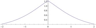
(a)

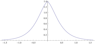
(b)

Figure 1. p=3 NLS with $\delta$ potential. $\alpha=1$; $\omega=1$ and $\omega=9$

Proposition 8.2.

For every $\alpha>0$ and for every $\omega>\alpha^{2}/4$ there exist exactly two solutions to (8.5), given by $\pm u_{\alpha,p,\omega}$, where the function $u_{\alpha,p,\omega}$ was defined in (2.10), (2.11).

Proof. According to Theorem 8.1 and by the continuity condition on $u$ (indeed we assume $u(x)\in H^{1}({\mathbb{R}})$) we deduce that either $u(x)>0$ or $u(x)<0$ for every $x\in{\mathbb{R}}$. We assume that $u(x)>0$ (the case $u(x)<0$ is similar).

Again by Theorem 8.1 there exist $x_{\pm}\in{\mathbb{R}}$ such that

$$u(x)=\varphi_{p,\omega}(x+x_{\pm}),\qquad x\in{\mathbb{R}}^{\pm},$$

where $\varphi_{p,\omega}$ was defined in (8.4).

By imposing the continuity condition at the the origin we deduce (due to the shape of the function $\varphi_{p,\omega}$), that $x_{+}=\pm x_{-}$. In the case $x_{+}=x_{-}=\tilde{x}$ we get $u(x)=\varphi_{p,\omega}(x+\tilde{x})$, that can be excluded since the derivative at the origin has no jump, so, as $\alpha>0$, the boundary condition in (8.5) is not satisfied. Hence we have $x_{+}=-x_{-}$. By the boundary condition imposed by (8.5) on the derivative of $u$, we deduce that, denoting $\tilde{x}=-x_{+}$,

$$\varphi_{p,\omega}^{\prime}(\tilde{x})-\varphi_{p,\omega}^{\prime}(-\tilde{x})=-\alpha\varphi_{p,\omega}(\tilde{x}),$$

namely

$$-2\sqrt{\omega}\Big{(}\frac{1}{\cosh^{2}(\frac{p-1}{2}\sqrt{\omega}\tilde{x})}\Big{)}^{\frac{1}{p-1}}\tanh(\frac{p-1}{2}\sqrt{\omega}\tilde{x})=-\alpha\Big{(}\frac{1}{\cosh^{2}(\frac{p-1}{2}\sqrt{\omega}\tilde{x})}\Big{)}^{\frac{1}{p-1}}$$

(where we used the even character of the function $\varphi_{\omega}$), i.e. $\tanh(\frac{p-1}{2}\sqrt{\omega}\tilde{x})=\frac{\alpha}{2\sqrt{\omega}}$. The proof is complete.

$\Box$

The stationary states for a $\delta$ interaction are represented in Figure 1.

We immediately have the following result (see [23])

Corollary 8.1.

The function

$$(\alpha^{2}/4,\infty)\ni\omega\rightarrow\|u_{\alpha,p,\omega}\|_{L^{2}({\mathbb{R}})}\in(0,\infty)$$

is continuous, increasing and surjective.

Proof.

Using (2.11), by direct computation one gets

$$\|u_{\alpha,p,\omega}\|_{L^{2}({\mathbb{R}})}^{2}\ =\ C(p)\omega^{\frac{5-p}{2p-2}}\int_{\frac{\alpha}{2\sqrt{\omega}}}^{1}(1-t^{2})^{\frac{3-p}{p-1}},$$

where $C(p)>0$ is independent of $\omega$, that is obviously a monotonically increasing function of $\omega$, approaching zero as $\omega$ vanishes, and going to infinity as $\omega$ goes to infinity. ∎

8.3. Stationary states for the $\delta^{\prime}$ interaction

We study the problem

$$\left\{\begin{array}[]{c}-u^{\prime\prime}+\omega u=u|u|^{p-1}\hbox{ on }{\mathbb{R}}\setminus\{0\},\ u(x)\in{\mathbb{R}},\ \omega\in{\mathbb{R}}\\ u\in H^{2}({\mathbb{R}}^{+})\oplus H^{2}({\mathbb{R}}^{-})\\ u(0-)-u(0+)=\beta u^{\prime}(0),u^{\prime}(0+)=u^{\prime}(0-)\\ u(0+)\cdot u(0-)<0\end{array}\right.$$ (8.6)

First, we prove a nonexistence result.

Proposition 8.3.

If $\omega\leq\beta^{2}/4$, then the problem to (8.6) admits the trivial solution $u\equiv 0$ only.

Proof. First notice that by Theorem 8.1 any solution $u$ to (8.6) consists of two pieces of solitons suitably matched at the origin. Moreover, by the boundary condition they have opposite sign on the real half-lines ${\mathbb{R}}^{\pm}$, so we can assume $u(x)>0$ on ${\mathbb{R}}^{+}$, being the case $u(x)<0$ equivalent. After multiplication of (8.6) by the function $\varphi_{\beta}(x)=\sqrt{\frac{2}{\beta}}({\mbox{sign}}x)e^{-\frac{2}{\beta}|x|}$ (that is a normalized eigenvector of the attractive $\delta^{\prime}$ interaction and was defined in the proof of Corollary 2.2), and integrating by parts twice, we get

$$-\frac{4}{\beta^{2}}\int v\cdot\varphi_{\beta}dx+\omega\int\varphi_{\beta}\cdot v\,dx\ =\ \int\varphi_{\beta}\cdot v|v|^{p-1}dx>0$$

where we have used the fact that $v\varphi_{\beta}$ has constant sign, and hence necessarily $\omega>\frac{\beta^{2}}{4}$.

$\Box$

Proposition 8.4.

Let $\beta>0$. Then, under the extra assumption

$$u(0+)=-u(0-)>0,$$ (8.7)

there exists a solution to (8.6) if and only if $\omega>\frac{4}{\beta^{2}}$. Moreover this solution is unique and equals $u_{odd,\beta,p,\omega}={\rm sign}(x)\varphi_{p,\omega}(x+\bar{x})$, where ${\rm sign}(x)$ is the sign function, $\varphi_{p,\omega}$ was defined in (8.4), and $\bar{x}=\bar{x}(\beta,p,\omega)>0$ solves the equation

$$\beta\sqrt{\omega}\tanh\left(\frac{p-1}{2}\sqrt{\omega}\bar{x}\right)=2,\ \bar{x}>0\ .$$

Proof. By Theorem 8.1 any solution $u$ that satisfies (8.6) plus the extra assumption $u(0+)>0$ has necessarily the following structure

$$\pm\varphi_{p,\omega}(x+\bar{x}),\qquad x\in{\mathbb{R}}^{\pm},$$

where $x_{\pm}$ are to be chosen in order to satisfy the boundary conditions in (8.6). Due to (8.7) and to the continuity of the derivative, we conclude $x_{+}=-x_{-}$. By introducing $x_{+}=\bar{x}$, the condition on the jump of $u$ at zero (see (7.8)) prescribes

$$\varphi_{p,\omega}(\bar{x})+\varphi_{p,\omega}(-\bar{x})=-\beta\varphi_{p,\omega}^{\prime}(\bar{x}),$$

or, more explicitly,

$$\frac{1}{\cosh^{\frac{2}{p-1}}(\frac{p-1}{2}\sqrt{\omega}\bar{x})}+\frac{1}{\cosh^{\frac{2}{p-1}}(\frac{p-1}{2}\sqrt{\omega}(-\bar{x}))}=\beta\sqrt{\omega}\frac{\tanh(\frac{p-1}{2}\sqrt{\omega}\bar{x})}{\cosh^{\frac{2}{p-1}}(\frac{p-1}{2}\sqrt{\omega}\bar{x})},$$

which implies $\bar{x}>0$.

The proof is complete. $\Box$

Proposition 8.5.

Let $\beta>0$. Then there exists a solution to (8.6) under the extra assumption

$$u(0+)>0\hbox{ and }u(0+)>|u(0-)|$$ (8.8)

if and only if $\omega>\frac{4}{\beta^{2}}\frac{p+1}{p-1}$. Moreover the solution to (8.6) that satisfies the extra assumptions (8.8) is unique and equals $u_{as,\beta,p,\omega}=\pm\varphi_{p,\omega}(x+x_{\pm}),x\in{\mathbb{R}}^{\pm}$, where the function $\varphi_{p,\omega}$ was defined in (8.4) and $x_{\pm}$ are the only solutions to the system

$$\left\{\begin{array}[]{c}\frac{\tanh(\frac{p-1}{2}\sqrt{\omega}x_{+})}{\cosh^{\frac{2}{p-1}}(\frac{p-1}{2}\sqrt{\omega}x_{+})}+\frac{\tanh(\frac{p-1}{2}\sqrt{\omega}x_{-})}{\cosh^{\frac{2}{p-1}}(\frac{p-1}{2}\sqrt{\omega}x_{-})}=0\\ \frac{1}{\cosh^{\frac{2}{p-1}}(\frac{p-1}{2}\sqrt{\omega}x_{+})}+\frac{1}{\cosh^{\frac{2}{p-1}}(\frac{p-1}{2}\sqrt{\omega}x_{-})}=\beta\sqrt{\omega}\frac{\tanh(\frac{p-1}{2}\sqrt{\omega}x_{+})}{\cosh^{\frac{2}{p-1}}(\frac{p-1}{2}\sqrt{\omega}x_{+})}\end{array}\right.$$ (8.9)

that satisfy the condition $x_{-}<0<x_{+}<|x_{-}|$.

Proof. By Theorem 8.1 any solution $u$ that satisfies (8.6) plus the extra assumption $u(0+)>0$ is necessarily of the type $\pm\varphi_{p,\omega}(\cdot+x_{\pm}),x\in{\mathbb{R}}^{\pm}$, where $x_{\pm}$ are to be chosen in order to satisfy the boundary conditions. It is also easy to check that under our assumptions necessarily $u^{\prime}(0)<0$ and hence $x_{+}>0$ and $x_{-}<0$. Moreover, since we are assuming $|u(0+)|>|u(0-)|$, then $x_{+}<|x_{-}|$. In fact, the boundary conditions are equivalent to

$$\varphi_{p,\omega}^{\prime}(x_{+})+\varphi_{p,\omega}^{\prime}(x_{-})=0$$

$$\varphi_{p,\omega}(x_{+})+\varphi_{p,\omega}(x_{-})=-\beta\varphi_{p,\omega}^{\prime}(x_{+}),$$

and system above rephrases as

$$\frac{\tanh(\frac{p-1}{2}\sqrt{\omega}x_{+})}{\cosh^{\frac{2}{p-1}}(\frac{p-1}{2}\sqrt{\omega}x_{+})}+\frac{\tanh(\frac{p-1}{2}\sqrt{\omega}x_{-})}{\cosh^{\frac{2}{p-1}}(\frac{p-1}{2}\sqrt{\omega}x_{-})}=0$$

$$\frac{1}{\cosh^{\frac{2}{p-1}}(\frac{p-1}{2}\sqrt{\omega}x_{+})}+\frac{1}{\cosh^{\frac{2}{p-1}}(\frac{p-1}{2}\sqrt{\omega}x_{-})}=\beta\sqrt{\omega}\frac{\tanh(\frac{p-1}{2}\sqrt{\omega}x_{+})}{\cosh^{\frac{2}{p-1}}(\frac{p-1}{2}\sqrt{\omega}x_{+})}$$

with the extra conditions

$$x_{-}<0<x_{+}<|x_{-}|.$$

According to Proposition 5.1, Lemma 5.2, and Theorem 5.3 in [4], to which we refer for details, the above system has a unique solution $(x_{+},x_{-})$. $\Box$

The situation is depicted in Figure 2, where the odd and asymmetric stationary states for a cubic NLS plus a $\delta^{\prime}$ interaction with $\beta=1$ and $\omega=64$ are represented.

Next, we collect some properties of the elements $u_{odd,\beta,p,\omega}$ and $u_{as,\beta,p,\omega}$ of the two families of standing waves of NLS with $\delta^{\prime}$ interaction.

Proposition 8.6.

The following properties hold:

• the function

  $$(4/\beta^{2},\infty)\ni\omega\rightarrow\|u_{odd,\beta,p,\omega}\|_{L^{2}({\mathbb{R}})}\in(0,\infty)$$

  is continuous, increasing and surjective;

• the function

  $$\left[\frac{4(p+1)}{\beta^{2}(p-1)},\infty\right)\ni\omega\rightarrow\|u_{as,\beta,p,\omega}\|_{L^{2}({\mathbb{R}})}\in[\|u_{odd,\beta,p,\frac{4(p+1)}{\beta^{2}(p-1)}}\|_{L^{2}({\mathbb{R}})},\infty)$$

  is continuous, increasing and surjective.

Proof. The result immediately follows from Proposition 6.5 in [4].

$\Box$

Next result is useful to compare energy and mass of stationary states $u_{odd,\beta,p,\omega}$ and $u_{as,\beta,p,\omega}$.

Proposition 8.7.

We have the following identities

$$\|u_{odd,\beta,p,\omega}\|_{L^{2}({\mathbb{R}})}^{2}=\Big{(}\frac{\omega(p+1)}{2}\Big{)}^{\frac{2}{p-1}}\frac{2}{(p-1)\sqrt{\omega}}\times$$

$$\left(\int^{1}_{-1}(1-t^{2})^{\frac{3-p}{p-1}}dt-\int_{-\frac{2}{\beta\sqrt{\omega}}}^{\frac{2}{\beta\sqrt{\omega}}}(1-t^{2})^{\frac{3-p}{p-1}}dt\right)$$

and

$$\|u_{as,\beta,p,\omega}\|_{L^{2}({\mathbb{R}})}^{2}=\Big{(}\frac{\omega(p+1)}{2}\Big{)}^{\frac{2}{p-1}}\frac{2}{(p-1)\sqrt{\omega}}\times$$

$$\left(\int^{1}_{-1}(1-t^{2})^{\frac{3-p}{p-1}}dt-\int_{\tanh(\frac{p-1}{2}\sqrt{\omega}x_{-})}^{\tanh(\frac{p-1}{2}\sqrt{\omega}x_{+})}(1-t^{2})^{\frac{3-p}{p-1}}dt\right)$$

Moreover, we have

$$\|u_{odd,\beta,p,\omega}\|_{L^{p+1}({\mathbb{R}})}^{p+1}=$$

$$\Big{(}\frac{\omega(p+1)}{2}\Big{)}^{\frac{(p+1)}{p-1}}\frac{2}{(p-1)\sqrt{\omega}}\left(\int^{1}_{-1}(1-t^{2})^{\frac{2}{p-1}}dt-\int_{-\frac{2}{\beta\sqrt{\omega}}}^{\frac{2}{\beta\sqrt{\omega}}}(1-t^{2})^{\frac{2}{p-1}}dt\right)$$

and

$$\|u_{as,\beta,p,\omega}\|_{L^{p+1}({\mathbb{R}})}^{p+1}=$$

$$\Big{(}\frac{\omega(p+1)}{2}\Big{)}^{\frac{(p+1)}{p-1}}\frac{2}{(p-1)\sqrt{\omega}}\left(\int^{1}_{-1}(1-t^{2})^{\frac{2}{p-1}}dt-\int_{-\tanh(\frac{p-1}{2}\sqrt{\omega}x_{-})}^{\tanh(\frac{p-1}{2}\sqrt{\omega}x_{+})}(1-t^{2})^{\frac{2}{p-1}}dt\right)$$

Proof. By looking at the expression of $u_{odd,\beta,p,\omega}(x)$ we get:

$$\|u_{odd,\beta,p,\omega}(x)\|_{L^{2}({\mathbb{R}})}^{2}=$$

$$\Big{(}\frac{\omega(p+1)}{2}\Big{)}^{\frac{2}{p-1}}\Big{(}\int_{\bar{x}}^{\infty}\frac{1}{\cosh^{\frac{4}{p-1}}(\frac{p-1}{2}\sqrt{\omega}x)}dx+\int^{-\bar{x}}_{-\infty}\frac{1}{\cosh^{\frac{4}{p-1}}(\frac{p-1}{2}\sqrt{\omega}x)}dx\Big{)}$$

$$=\Big{(}\frac{\omega(p+1)}{2}\Big{)}^{\frac{2}{p-1}}\frac{2}{(p-1)\sqrt{\omega}}\Big{(}\int_{\frac{p-1}{2}\sqrt{\omega}\bar{x}}^{\infty}\frac{1}{\cosh^{\frac{4}{p-1}}(x)}dx+\int^{-\frac{p-1}{2}\sqrt{\omega}\bar{x}}_{-\infty}\frac{1}{\cosh^{\frac{4}{p-1}}(x)}dx\Big{)}$$

and after the change of variable $t=\tanh x$ we get

$$\|u_{odd,\beta,p,\omega}(x)\|_{L^{2}({\mathbb{R}})}^{2}=\Big{(}\frac{\omega(p+1)}{2}\Big{)}^{\frac{2}{p-1}}\frac{2}{(p-1)\sqrt{\omega}}\times$$

$$\left(\int^{1}_{\tanh(\frac{p-1}{2}\sqrt{\omega}\bar{x})}(1-t^{2})^{\frac{3-p}{p-1}}dt+\int_{-1}^{-\tanh(\frac{p-1}{2}\sqrt{\omega}\bar{x})}(1-t^{2})^{\frac{3-p}{p-1}}dt\right)$$

The other identities can be proved in the same way.

$\Box$

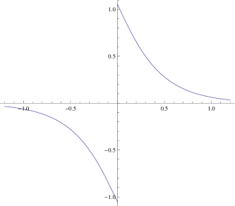
(a)

(b)

Figure 2. p=3 NLS with $\delta^{\prime}$: $u_{odd}$ and $u_{as}$ for $\beta=1$, $\omega=64.$

8.4. Stationary states for the dipole interaction

We study

$$\left\{\begin{array}[]{c}-u^{\prime\prime}+\omega u=u|u|^{p-1}\hbox{ on }{\mathbb{R}}\setminus\{0\},u(x)\in{\mathbb{R}},\omega>0\\ u\in H^{2}({\mathbb{R}}^{-})\oplus H^{2}({\mathbb{R}}^{+})\\ u(0+)=\tau u(0-),\tau u^{\prime}(0+)=u^{\prime}(0-)\end{array}\right.$$ (8.10)

Proposition 8.8.

For every $\tau>0$ and $\omega>0$ there exist exactly two solutions to (8.10) under the extra assumption

$$u(0+)>0$$

Moreover, the solutions have the following structure

$$\chi_{\tau,p,\omega}^{+}(x)=\left(\frac{\omega(p+1)}{2\cosh^{2}(\frac{p-1}{2}\sqrt{\omega}(x+\xi_{\pm}))}\right)^{\frac{1}{p-1}}\hbox{ for }x\in{\mathbb{R}}^{\pm}$$

$$\chi_{\tau,p,\omega}^{-}(x)=\left(\frac{\omega(p+1)}{2\cosh^{2}(\frac{p-1}{2}\sqrt{\omega}(x-\xi_{\pm}))}\right)^{\frac{1}{p-1}}\hbox{ for }x\in{\mathbb{R}}^{\pm}$$

where $\xi_{\pm}=\xi_{\pm}(\tau,p,\omega)\in{\mathbb{R}}$ are defined by the following conditions:

$$\tanh\left(\frac{p-1}{2}\sqrt{\omega}\xi_{+}\right)=\sqrt{\frac{1-\tau^{p-1}}{1-\tau^{p+3}}}$$

$$\tanh\left(\frac{p-1}{2}\sqrt{\omega}\xi_{-}\right)=\tau^{2}\sqrt{\frac{1-\tau^{p-1}}{1-\tau^{p+3}}}$$

Proof. By Theorem 8.1 any solution $u(x)$ that satisfies (8.10) plus the extra assumption $u(0+)>0$ has necessarily the following structure

$$u(x)=\left(\frac{\omega(p+1)}{2\cosh^{2}(\frac{p-1}{2}\sqrt{\omega}(x+y_{\pm})}\right)^{\frac{1}{p-1}}\hbox{ for }x\in{\mathbb{R}}^{\pm}$$

where $y_{\pm}$ have to be chosen in order to satisfy the boundary conditions.

$$\tau\varphi_{p,\omega}^{\prime}(y_{+})-\varphi_{p,\omega}^{\prime}(y_{-})=0$$

$$\varphi_{p,\omega}(y_{+})-\tau\varphi_{p,\omega}(y_{-})=0$$

where $\varphi_{p,\omega}$ is given in (8.4). The above system is equivalent to:

$$\tau\frac{\tanh(\frac{p-1}{2}\sqrt{\omega}y_{+})}{\cosh^{\frac{2}{p-1}}(\frac{p-1}{2}\sqrt{\omega}y_{+})}-\frac{\tanh(\frac{p-1}{2}\sqrt{\omega}y_{-})}{\cosh^{\frac{2}{p-1}}(\frac{p-1}{2}\sqrt{\omega}y_{-})}=0$$

$$\frac{1}{\cosh^{\frac{2}{p-1}}(\frac{p-1}{2}\sqrt{\omega}y_{+})}-\tau\frac{1}{\cosh^{\frac{2}{p-1}}(\frac{p-1}{2}\sqrt{\omega}y_{-})}=0$$

By introducing $t_{\pm}=\tanh(\frac{p-1}{2}\sqrt{\omega}y_{\pm})$ and by the well-known identity $\frac{1}{\cosh^{2}x}=1-\tanh^{2}x$ the system above is equivalent to

$$\left\{\begin{array}[]{c}\tau^{2}t_{+}=t_{-}\\ (1-t_{+}^{2})=\tau^{p-1}(1-t_{-}^{2})\end{array}\right.$$ (8.11)

and hence the conclusion easily follows.

$\Box$

The ground states of a dipole interaction with various values of $\tau$ and $\omega=1$ are represented in Figure 3.

(a)

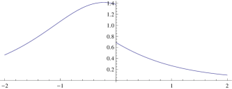
(b)

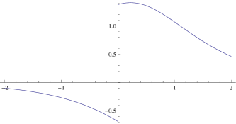
(c)

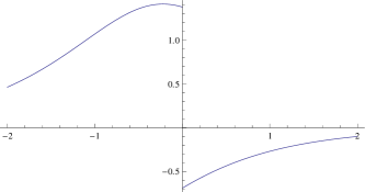
(d)

Figure 3. Ground states for the $p=3$ NLS with dipole.

The following property allows to compare energy and mass of stationary states the of $H_{tau}^{dip}$.

Proposition 8.9.

Assume $\tau>1$ and $\chi^{\pm}_{\tau,p,\omega}$ as in Proposition 8.8, then we have the following identities:

$$\|\chi^{\pm}_{\tau,p,\omega}\|_{L^{2}({\mathbb{R}})}^{2}=$$ (8.12)

$$\Big{(}\frac{\omega(p+1)}{2}\Big{)}^{\frac{2}{p-1}}\frac{2}{(p-1)\sqrt{\omega}}\left(\int_{-1}^{1}(1-t^{2})^{\frac{3-p}{p-1}}\pm\int^{\tau^{2}\sqrt{\frac{1-\tau^{p-1}}{1-\tau^{p+3}}}}_{\sqrt{\frac{1-\tau^{p-1}}{1-\tau^{p+3}}}}(1-t^{2})^{\frac{3-p}{p-1}}dt\right)$$

$$\|\chi^{\pm}_{\tau,p,\omega}\|_{L^{p+1}({\mathbb{R}})}^{p+1}=$$ (8.13)

$$\Big{(}\frac{\omega(p+1)}{2}\Big{)}^{\frac{(p+1)}{p-1}}\frac{2}{(p-1)\sqrt{\omega}}\left(\int^{1}_{-1}(1-t^{2})^{\frac{2}{p-1}}dt\pm\int_{\sqrt{\frac{1-\tau^{p-1}}{1-\tau^{p+3}}}}^{\tau^{2}\sqrt{\frac{1-\tau^{p-1}}{1-\tau^{p+3}}}}(1-t^{2})^{\frac{2}{p-1}}dt\right)$$

Proof. We prove (8.12). By looking at the explicit expression of $\chi^{+}_{\tau,p,\omega}$ we get

$$\|\chi^{+}_{\tau,p,\omega}\|_{L^{2}({\mathbb{R}})}^{2}=$$

$$\Big{(}\frac{\omega(p+1)}{2}\Big{)}^{\frac{2}{p-1}}\Big{(}\int_{\xi_{+}}^{\infty}\frac{1}{\cosh^{\frac{4}{p-1}}(\frac{p-1}{2}\sqrt{\omega}x)}dx+\int^{\xi_{-}}_{-\infty}\frac{1}{\cosh^{\frac{4}{p-1}}(\frac{p-1}{2}\sqrt{\omega}x)}dx\Big{)}$$

$$=\Big{(}\frac{\omega(p+1)}{2}\Big{)}^{\frac{2}{p-1}}\frac{2}{(p-1)\sqrt{\omega}}\Big{(}\int_{\frac{p-1}{2}\sqrt{\omega}\xi_{+}}^{\infty}\frac{1}{\cosh^{\frac{4}{p-1}}(x)}dx+\int^{\frac{p-1}{2}\sqrt{\omega}\xi_{-}}_{-\infty}\frac{1}{\cosh^{\frac{4}{p-1}}(x)}dx\Big{)}$$

and after the change of variable $t=\tanh x$ we get

$$\|\chi^{+}_{\tau,p,\omega}\|_{L^{2}({\mathbb{R}})}^{2}=\Big{(}\frac{\omega(p+1)}{2}\Big{)}^{\frac{2}{p-1}}\frac{2}{(p-1)\sqrt{\omega}}\times$$

$$\left(\int^{1}_{\sqrt{\frac{1-\tau^{p-1}}{1-\tau^{p+3}}}}(1-t^{2})^{\frac{3-p}{p-1}}dt+\int_{-1}^{\tau^{2}\sqrt{\frac{1-\tau^{p-1}}{1-\tau^{p+3}}}}(1-t^{2})^{\frac{3-p}{p-1}}dt\right)$$

By a similar argument we can treat $\|\chi^{-}_{\tau,p,\omega}\|_{L^{2}({\mathbb{R}})}^{2}$ and we can also deduce (8.13).

$\Box$

References

- [1] Adami R., Cacciapuoti C., Finco D., Noja D.: Fast solitons on star graphs, Rev. Math. Phys, 23, 4, 409–451 (2011).
- [2] Adami R., Cacciapuoti C., Finco D., Noja D.: Stationary states of NLS on star graphs, arXiv:1104.3839, submitted (2011).
- [3] Adami R., Noja D.: Existence of dynamics for a 1-d NLS equation perturbed with a generalized point defect, J. Phys. A Math. Theor. 42, 49, 495302, 19pp (2009).
- [4] Adami R., Noja D.: Stability and symmetry breaking bifurcation for the ground states of a NLS equation with a interaction, arXiv:1112.1318, Comm. Math. Phys., in print (2012).
- [5] Adami R., Noja D., Sacchetti A.: On the mathematical description of the effective behaviour of one-dimensional Bose-Einstein condensates with defects, in Bose-Einstein Condensates: Theory, Characteristics, and Current Research, Nova Publishing, New York (2010).
- [6] Akhiezer N., Glazman I.: Theory of linear operators in Hilbert spaces, New York, Ungar (1963).
- [7] Albeverio S., Brzeźniak Z., Dabrowski L.: Fundamental solutions of the Heat and Schrödinger Equations with point interaction, J. Func. An., 130, 220-254 (1995).
- [8] Albeverio S., Gesztesy F., Høgh-Krohn R., Holden H.: Solvable Models in Quantum Mechanics, ed., with an appendix of P. Exner, AMS, Providence (2005).
- [9] Albeverio S., Kurasov P.: Singular Perturbations of Differential Operators, Cambridge University Press (2000).
- [10] Bellazzini J., Visciglia N.: On the orbital stability for a class of nonautonmous NLS, Indiana Univ. Math. J., 59, 1211-1230 (2010).
- [11] Berestycki H., Lions P.-L.: Nonlinear scalar field equations, I - Existence of a ground state., Arch. Rat. Mech. Anal., 82, 313–345 (1983).
- [12] Blank J., Exner P., Havlicek M.: Hilbert spaces operators in Quantum Physics, Springer, New York (2008).
- [13] Brezis H., Lieb E. H.: A relation between pointwise convergence of functions and convergence of functionals, Proc. Amer. Math. Soc., 88, 486–490 (1983).
- [14] Cao Xiang D., Malomed A. B.: Soliton defect collisions in the nonlinear Schrödinger equation, Phys. Lett. A, 206, 177–182 (1995).
- [15] Cazenave T.: Semilinear Schrödinger Equations, vol. 10 Courant Lecture Notes in Mathematics, AMS, Providence (2003).
- [16] Cazenave T., Lions P.-L.: Orbital stability of standing waves for some nonlinear Schrödinger equations, Comm. Math. Phys., 85, 549–561 (1982).
- [17] Cheon T., Shigehara T.: Realizing discontinuous wave functions with renormalized short-range potentials, Phys. Lett. A 243, 111–116 (1998).
- [18] Datchev K., Holmer J.: Fast soliton scattering by attractive delta impurities, Comm. Part. Diff. Eq. 34, 1074–1113 (2009).
- [19] Deift P., Park J.: Long-Time Asymptotics for Solutions of the NLS Equation with a Delta Potential and Even Initial Data, Int. Math. Res. Notices, 24, 5505–5624 (2011).
- [20] Exner P., Grosse P.: Some properties of the one-dimensional generalized point interactions (a torso), mp-arc 99-390, math-ph/9910029 (1999).
- [21] Exner P., Neidhardt H., Zagrebnov V.A.: Potential approximations to a : an inverse Klauder phenomenon with norm-resolvent convergence, Comm. Math. Phys., 224, 593–612 (2001).
- [22] Fukuizumi R., Jeanjean L.: Stability of standing waves for a nonlinear Schrödinger equation with a repulsive Dirac delta potential, Disc. Cont. Dyn. Syst. (A), 21, 129–144 (2008).
- [23] Fukuizumi R., Ohta M., Ozawa T.: Nonlinear Schrödinger equation with a point defect, Ann. Inst. H. Poincaré, Anal. Non Linéaire, 25, 837–845 (2008).
- [24] Furuhashi Y., Hirokawa M., Nakahara K., Shikano Y.: Role of a phase factor in the boundary condition of a one-dimensional junction, J. Phys. A Math. Theor., 43, 354010, 17 pp, (2010).
- [25] Golovaty Yu. D., Hryniv R. O.: On norm resolvent convergence of Schrödinger operators with -like potentials, J. Phys. A Math. Theor., 44, 049802 (2011); Corrigendum J. Phys. A Math. Theor. 44, 049802 (2011).
- [26] Goodman R. H., Holmes P. J., Weinstein M.I.: Strong NLS soliton-defect interactions, Physica D, 192, 215–248 (2004).
- [27] Grillakis M., Shatah J., Strauss W.: Stability theory of solitary waves in the presence of symmetry - I, J. Func. An., 74, 160–197 (1987).
- [28] Grillakis M., Shatah J., Strauss W.: Stability theory of solitary waves in the presence of symmetry - II, J. Func. An., 94, 308–348 (1990).
- [29] Holmer J., Marzuola J., Zworski M.: Fast soliton scattering by delta impurities, Comm. Math. Phys, 274, 187–216 (2007).
- [30] Holmer J., Zworski M.: Breathing patterns in nonlinear relaxation, Nonlinearity, 22, 1259–1301, (2009).
- [31] Le Coz S., Fukuizumi R., Fibich G., Ksherim Y., Sivan Y.: Instability of bound states of a nonlinear Schrödinger equation with a Dirac potential, Physica D, 237, 1103–1128 (2008).
- [32] Linzon Y., Morandotti R., Aimez V., Ares V., Bar-Ad S.: Nonlinear scattering and trapping by local photonic potentials, Phys. Rev. Lett. 99, 133901 (2007).
- [33] Reed M., Simon B.: Methods of modern Mathematical Physics, Vol I, Academic Press. (1980).
- [34] Weinstein M.: Modulational stability of ground states of nonlinear Schroedinger equations, SIAM J. Math. Anal., 16, 472–491 (1985).
- [35] Weinstein M.: Lyapunov stability of ground states of nonlinear dispersive evolution equations, Comm. Pure Appl. Math., 39, 51–68 (1986).
- [36] Witthaut D., Mossmann S., Korsch H. J.: Bound and resonance states of the nonlinear Schrödinger equation in simple model systems, J. Phys. A Math. Gen., 38, 1777–1702 (2005).
- [37] Zolotaryuk A. V., Christiansen P.L., Iermakova S. V.: Scattering properties of point dipole interactions, J. Phys. A Math. Gen. 39, 9329–9338 (2006).
- [38] Zolotaryuk A. V.: Boundary conditions for the states with resonant tunnelling across the -potential: Phys. Lett. A 374, 1636–1641 (2010).