A framework for solvation in quantum Monte Carlo

Abstract

Employing a classical density-functional description of liquid environments, we introduce a rigorous method for the diffusion quantum Monte Carlo calculation of free energies and thermodynamic averages of solvated systems that requires neither thermodynamic sampling nor explicit solvent electrons. We find that this method yields promising results and small convergence errors for a set of test molecules. It is implemented readily and is applicable to a range of challenges in condensed matter, including the study of transition states of molecular and surface reactions in liquid environments.

The physics of solvation, though poorly understood, plays a critical role in a wide range of systems from the biological to the technological. For example, the pathways in protein folding Lazaridis:1997p502 ; Rhee:2004p503 ; FernandezEscamilla:2004p501 and transition states of ionic reactions Kim:2009p515 ; Regan:2002p516 are known to be highly solvent dependent. Development of a fundamental understanding of the kinetics which underlie such processes requires an accurate description of the quantum mechanical processes involved in bond breaking and formation in solution.

Unlike less rigorous electronic structure methods, quantum Monte Carlo methods Foulkes:2001p332 do provide the required accuracy for transition states, reactants, and products needed to give reliable information on reaction pathways. However, a full quantum Monte Carlo treatment, in principle, requires solving Schrödinger’s equation for all of the involved solvent molecules, a difficulty radically compounded by the need to sample the phase-space of all thermodynamically relevant configurations of the solvent. This Communication introduces a framework for the treatment of solvation in diffusion Monte Carlo which completely eliminates the need for explicit solvent electrons and such phase-space sampling, while remaining completely ab initio and exact in principle — in the same sense in which density-functional theory meets these criteria.

Previous attempts to model the effects of solvation in quantum Monte Carlo fall into two categories: (i) simulation of the environment through molecular dynamics Cho:2010p492 ; Grossman:2005p498 , and (ii) introduction of a polarizable continuum Amovilli:2006p491 ; Amovilli:2008p495 . The former approach, in principle, captures molecular-scale effects such as solvation shells and non-local dielectric response. However, molecular dynamics with empirical potentials Cho:2010p492 , though benefiting from a simplified description of the solvent, depends on a highly parameterized potential to describe the interactions between molecules. Additionally, such calculations require phase-space sampling, which makes the calculations costly — especially if individual electronic structure calculations for the solute are needed for each fluid configuration. Approaches have been proposed to mitigate this expense within ab initio molecular dynamics calculations Grossman:2005p498 , but this approach also is extremely expensive due to the need to include of all of the solvent electrons and nuclei.

In contrast, the polarizable continuum model (PCM) is a computationally inexpensive tool for approximating solvation energies without phase-space sampling. Unfortunately, this model lacks theoretical justification for the treatment of water as a continuum on molecular length scales, and so does not constitute a truly ab initio method. Indeed, the pioneering work on solvation studies within diffusion Monte Carlo electronic structure methods Amovilli:2008p495 rested on the ad hoc introduction of a polarizable medium and required a set of spheres with radii determined empirically. A further, practical disadvantage of the aforementioned PCM approach is that it requires potentially costly statistical evaluation of solvent potentials, and so it has yet to yield meaningful comparisons between predicted solvation energies and experiment.

Joint density-functional theory Petrosyan:2005p493 circumvents both the inaccuracies inherent in the polarizable continuum model and empirical molecular dynamics and the expense associated with ab initio molecular dynamics. This work presents an integrated approach to quantum Monte Carlo calculations within this new, rigorous statistical treatment of the solvent, and introduces a variational theorem which abrogates much of the computational complexity associated with achieving full self-consistency between the solute and the solvent. While our approach in theory requires no adjustable parameters, we employ a simplified, approximate version of the theory in this first demonstration that does require a single empirically adjusted parameter.

This Communication begins with a brief review of joint density-functional theory and then describes a quantum Monte Carlo formulation of that theory, compares predictions to solvation data, and shows that self-consistency to within chemical accuracy is achievable with the computational cost of a single quantum Monte Carlo calculation.

Joint density-functional theory and quantum Monte Carlo. Joint density-functional theory Petrosyan:2005p493 ; Petrosyan:2007 states that, in principle, the exact quantum and thermodynamically averaged electronic and nuclear densities and the exact free energy of a solvated system can be obtained by minimization of a universal free-energy functional, without the need to sample explicitly the phase space of all possible configurations of solvent molecules. This minimization is carried out over all realizable average solute electron densities $n(r)$ and average solvent site densities $N_{\alpha}(r)$. (In the present work, $N_{\alpha}(r)$ refers to the single-particle densities of the oxygen nuclei and protons comprising the solvent, water.) Note that $n(r)$ here refers only to the electron density of the solute because the electron density of the solvent need not be considered explicitly. Naturally, the underlying indistinguishability of electrons implies that there is no unique decomposition of the total electron density into solute and solvent contributions. Consequently, the solution to the minimization problem is highly degenerate with many choices for $n(r)$ leading to the same, exact free energy. This complication notwithstanding, the free energy and $N_{\alpha}(r)$ obtained at the minimum are meaningful and represent the exact free energy and solvent site distribution of the combined system at equilibrium. (See Ref. Petrosyan:2007 for a fuller discussion.) Finally, we note that the exact universal functional conveniently decomposes into a sum of three terms,

$$A[n,\{N_{\alpha}\}]=A_{\textrm{HK}}[n]+\Phi_{\textrm{lq}}[\{N_{\alpha}\}]+\Delta A[n,\{N_{\alpha}\}],$$ (1)

where $A_{\textrm{HK}}[n]$ is the electronic Hohenberg-Kohn free-energy functional for the explicit system in isolation, $\Phi_{\textrm{lq}}$ is the free-energy functional for the liquid when in isolation, and $\Delta A$ represents the coupling between the explicit system and the solvent. Note that, essentially being the definition of $\Delta A[n,\{N_{\alpha}\}]$, Eq. (1) is exact.

Although Eq. (1) is exact in principle, the forms of these three functionals on the right-hand side are unknown and need to be approximated in practice. Generally, such approximations will break the aforementioned degeneracy and select a specific $n(r)$ at the minimum of the approximated functional. In this Communication, we use diffusion Monte Carlo to describe the term $A_{\textrm{HK}}[n]$, and, for our quantum Monte Carlo implementation of joint density-functional theory, we write the terms related to the environment as

$$A_{\textrm{env}}[n]\equiv\min_{\{N_{\alpha}\}}{\left(\Phi_{\textrm{lq}}[\{N_{\alpha}\}]+\Delta A[n,\{N_{\alpha}\}]\right)}.$$ (2)

The variational derivative of Eq. (1) with respect to the exact electron density then yields the Euler-Lagrange equation $0=\delta A/\delta n=\delta(A_{HK}+A_{\textrm{env}})/\delta n$, which is precisely the equation for the isolated solute system in an external potential $V_{\textrm{env}}\equiv\delta A_{\textrm{env}}[n]/\delta n$. When an external potential is found for which the electron density $n(r)$ apportioned to the solute yields back the same potential through this definition, the self-consistent, exact thermodynamic state of the system will have been found. In principle, this exact solution can be obtained through multiple self-consistent iterations. The main difficulty of a quantum Monte Carlo implementation of $A_{\textrm{HK}}$ in this process is the presence of statistical noise in the resulting electron densities, particularly in regions of low electron density, a problem which also plagues the approach of Ref. Amovilli:2008p495 . There has been recent progress in reducing this noise Assaraf:2007p518 , but the results are not yet sufficiently clean for use in self-consistent calculations. We therefore now introduce a method to estimate the self-consistent solution of our solvation theory without evaluation of the electron density within quantum Monte Carlo.

First-order estimator of self-consistency. A natural starting point for a joint density-functional theory quantum Monte Carlo calculation is a fully self-consistent joint density-functional theory calculation within the local density (LDA) or generalized gradient (GGA) approximation for $A_{\textrm{HK}}$. Such calculations provide trial wavefunctions for quantum Monte Carlo calculations, and the resulting densities $n_{\textrm{DFT}}$ give estimates for the environment potential $\tilde{V}_{\textrm{env}}=\delta A_{\textrm{env}}[n_{\textrm{DFT}}]/\delta n$. One can then perform a single quantum Monte Carlo calculation of the solute within this estimated potential, yielding both an initial quantum Monte Carlo density $n_{\textrm{QMC}}$ and energy $A_{\textrm{QMC}}[n_{\textrm{QMC}}]$. Note that the latter quantity is defined as the quantum Monte Carlo estimate of the functional $A_{HK}$; i.e., the energy of the solute without the energy associated with $\tilde{V}_{\textrm{env}}$.

The two calculations described in the above paragraph could then be combined to give a zeroth-order estimate of the free energy of the solvated system as $A_{\textrm{QMC}}[n_{\textrm{QMC}}]+A_{\textrm{env}}[n_{\textrm{DFT}}]$. This, however, loses the benefits of the variational principle because the two terms are not self-consistent in that they are evaluated at different electron densities, and so the resulting estimate is not necessarily an upper bound for the final, converged result. Also, the resulting error is first-order in the errors in the density, rather than second-order, as is usually associated with variational calculations. We can correct for this by evaluating, with errors only in the second-order, $A_{env}[n_{\textrm{QMC}}]=A_{env}[n_{\textrm{DFT}}]+\int d^{3}r\,\tilde{V}_{env}\,(n_{\textrm{QMC}}-n_{\textrm{DFT}})$ because, by definition, $\tilde{V}_{\textrm{env}}=\delta A_{\textrm{env}}[n_{\textrm{DFT}}]/\delta n$. The final result equals

$$A= A_{\textrm{QMC}}[n_{\textrm{QMC}}]+A_{\textrm{env}}[n_{\textrm{DFT}}]+$$ (3)

$$\int d^{3}r\tilde{V}_{\textrm{env}}(r)\left(n_{\textrm{QMC}}(r)-n_{\textrm{DFT}}(r)\right)+{\cal O}(\delta n^{2}),$$

with errors that are second-order in both the difference between the exact converged density and the density-functional theory density $n_{\textrm{DFT}}$ and the difference between the exact converged density and the first-iteration density $n_{\textrm{QMC}}$. Below, we show that this new approach is operationally nearly as good as full self-consistency, but with the effort of only a single quantum Monte Carlo calculation.

Implementation. In this work we demonstrate our solvation technique with a simplified description of the environment, but we stress that it may be employed just as readily with whatever functionals for the liquid become available. We note that the quality of our results now depend on our approximation for $A_{env}$, which we hope to improve in the future. Specifically, we here employ the isodensity model of Petrosyan et al. Petrosyan:2005p493 , which is similar to the dielectric model by Fattebert and Gygi Fattebert:2003p497 . These models take the dielectric constant to be a local function of the electron density that switches smoothly from the value for vacuum at high solute electron densities to the dielectric constant of the bulk liquid for low electron densities. This simplified joint density-functional is similar in spirit to the smoothly transitioning nonlinear polarizable continuum model described in Ref. Amovilli:2006p491 , but here we work in a rigorous framework and also effectively achieve solute-solvent self-consistency. We have implemented our method in the open source code JDFTx jdftx , interfaced with CASINO Needs:2008p339 . In anticipation of applying our method to large solvated surfaces, we use for our starting point the computationally inexpensive local-density approximation at full solute-solvent self-consistency. Fig. 1(a) illustrates the cavity formation for acetone, a small molecule chosen for its well-known experimental solvation energy. Our reported solvation energies include, in addition to the electrostatic components from our simplified electrostatic functional, the cavitation energy shown in Table 1, estimated from classical density functional theory following the procedure in Ref. 2011arXiv1112.1442S as included in the JDFTx package jdftx and employing a functional based on Ref. jefferyAustin .

The density-functional theory and Hartree-Fock calculations employ pseudopotentials from Burkatzki et al. Burkatzki:2007p451 and expand the wave functions in a plane-wave basis with a cutoff energy of 30 H (hartree). The local density approximation is employed for the density functional theory calculations, performed using JDFTx jdftx , and a simulation box of 40 ${\mathrm{bohr}^{3}}$. The quantum Monte Carlo calculations are performed using CASINO Needs:2008p339 and employ a trial wavefunction of a product of a single Slater determinant of density functional orbitals and a Jastrow correlation factor composed of electron-nucleus and electron-electron terms with expansion order eight, and electron-electron-nucleus terms with expansion order three, as described in Ref. jastrow . The orbitals and external potential $V_{\mathrm{env}}$ are represented by B-splines. The parameters of the Jastrow factor are optimized by variance minimization VarMin . The diffusion Monte Carlo time step is 0.01 H^-1. (Going from 0.01 to 0.001 H^-1, we found the time-step error to be within the statistical uncertainty we report for the solvation energy for acetone in Figure 1, with the solvation parameter $\mathrm{n_{c}}=7$ x $10^{-4}~{}\mathrm{bohr}^{-3}$.) Molecular geometries are from the Computational Chemistry Comparison and Benchmark Database: either from experimental data if available, or density-functional optimization using the B3LYP functional and the cc-pVTZ basis set NIST .

(a)

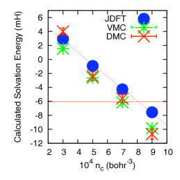
(b)

Figure 1: (Color Online) (a) Joint density-functional theory description of acetone in aqueous solution: electron density contours as green (gray) surfaces, solvent as solid purple (dark gray). (b) Solvation energies for acetone: diffusion Monte Carlo (DMC) as red (gray) x’s, variational Monte Carlo (VMC) as green (gray) strikethrough x’s, Joint Density Functional Theory (JDFT) as blue (gray) circles, Joint Density Functional Theory best fit as a dashed black line, and experiment as a horizontal red (gray) line.

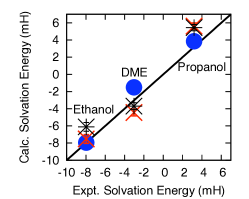
Figure 2: (Color Online) Theoretical versus experimental solvation energies for ethanol, dimethyl ether (DME), propane (left to right): Joint Density Functional Theory as blue (gray) circles, zeroth-order diffusion Monte Carlo as black strikethrough x’s, first-order corrected diffusion Monte Carlo as red (gray) x’s. Experimental values from Barone:1997p507 .

$10^{4}$ $\mathrm{n_{c}}$ ($\mathrm{bohr}^{-3}$)	3.0	5.0	7.0	8.1	9.0
dimethyl ether	9.0	7.8	7.0	6.7	6.5
ethanol	8.9	7.7	7.0	6.7	6.4
propane	10.3	8.9	8.0	7.7	7.5
acetone	10.6	9.2	8.3	8.0	7.7

Table 1: Formation energies (mH) for cavities at various values of the electron isodensity-contour parameter $n_{c}$ from the model of Ref. Petrosyan:2005p493 , based on the cavitation energy method of Ref. 2011arXiv1112.1442S .

For the continuum description of water, we use the local dielectric function $\epsilon(n(r))=1+(\epsilon_{\textrm{b}}-1)\,\textrm{erfc}\left(\textrm{ln}(\frac{n(r)}{n_{c}})/(\sqrt{2}\sigma)\right)/2$, where $\epsilon_{\textrm{b}}$ is the bulk dielectric constant of the fluid, $n_{c}$ specifies the value of the solute electron density at which the dielectric cavity forms, and $\sigma$ controls the transition width Petrosyan:2005p493 . This description of water leads to the expression $A_{env}[n_{\textrm{DFT}}]=\frac{1}{2}\int dr^{3}(n_{\textrm{DFT}}-N)(-4\pi(\nabla\cdot\epsilon(n_{\textrm{DFT}})\nabla)^{-1}+4\pi(\nabla^{2})^{-1})(n_{\textrm{DFT}}-N)$, where $N$ represents the nuclei of the solute.

Results. Figure 1(b) shows the resulting solvation energies for acetone as a function of $n_{c}$. The results are not sensitive to $\sigma$, so we leave this value fixed at 0.6 and optimize the values of $n_{c}$ for use in diffusion Monte Carlo. All of the variational Monte Carlo results and nearly all the diffusion Monte Carlo results lie below the density-functional theory data. The variational Monte Carlo results with no Jastrow factor (and thus no correlation, but exact exchange energy) and the diffusion Monte Carlo results lie very near to each other, indicating that the primary corrections in solvation energy to the density-functional results come from the exact treatment of the exchange and that corrections to correlation beyond the local-density approximation largely cancel for the solvation energies, at least for acetone.

A least squares fit of the data shown in Fig. 1b yields $n_{c}=7.0\times 10^{-4}$ $\mathrm{bohr}^{-3}$ as optimal for diffusion Monte Carlo and $n_{c}=8.1\times 10^{-4}$ $\mathrm{bohr}^{-3}$ as optimal for use with density-functional theory. Figure 2 shows the resulting solvation energies of three molecules for both the zeroth-order expression and the first-order corrected version from Eq. (3). The agreement between the quantum Monte Carlo results and experiment is encouraging given the particularly simple model employed here for the fluid. The figure also demonstrates the importance of using Eq. (3) to include the effects of self-consistency, particularly for ethanol.

To estimate the remaining error between the corrected formula (Eq. (3)) and full self-consistency, we employ two different electronic structure methods for which achievement of full self-consistency is feasible and whose difference in densities we expect to be similar to the density difference between density-functional theory and quantum Monte Carlo. We begin with an environment potential $V_{env}$ from a solvated density-functional theory (Hartree-Fock) calculation, and include it in a Hartree Fock (density-functional theory) calculation, attempting to predict the final self-consistent energy using our proposed methods. Fig. 3 compares the zeroth and first-order corrected approximations with the fully self-consistent results when working this procedure in both directions.

The data exhibit a number of behaviors which we expect to be general trends. First, the first-order corrected data lie above the fully self-consistent result, regardless of the starting point. Second, the remaining (second-order and higher) errors are all quite small (0.2 mH or less) and on the order of about one-third the size of the first-order correction. Third, the remaining errors in the corrected results for a given molecule when going in either direction between density-functional theory and Hartree Fock are nearly identical. The difference between these remaining errors gives an estimate of the correction at odd orders (third and higher), indicating that the errors remaining are dominated by the second-order term. In aqueous solution, electrostatic screening, a negative-definite quantity, dominates this second-order term, thus explaining why the corrected results generally lie above the self-consistent solution.

These observations strongly suggest that the self-consistency error in our corrected diffusion Monte Carlo results is less than one mH for ethanol, and even less for the other molecules. Our procedure thus likely gives an upper bound well within chemical accuracy of the results of full self-consistency, with the need for only a single quantum Monte Carlo calculation.

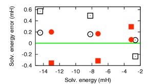
Figure 3: (Color Online) Zeroth order approximation errors (squares) and first order approximation errors from Eq. (3) (circles) relative to the exact self-consistent fluid-electronic structure minimization for Hartree-Fock calculations with LDA potentials in black (unfilled) and LDA calculations with Hartree-Fock potentials in red (gray) (filled), for the electrostatic solvation energies of ethanol, dimethyl ether, and propane (from left to right).

Conclusion. The framework of joint density-functional theory provides a rigorous and efficient method for solvation in quantum Monte Carlo, without the need for phase-space sampling of the fluid. Moreover, a special procedure allows self-consistency of the joint calculation to be obtained (along with an estimate of the remaining errors) to within chemical accuracy, all at the cost of only a single quantum Monte Carlo total-energy calculation carried out in a fixed external potential. This solvation method applies just as readily to molecular and surface calculations. The procedure is general and may be used not only with quantum Monte Carlo but other correlated total-energy methods as well.

K.A.S. and K.L.W were supported by National Science Foundation Graduate Research Fellowships, K.A.S. and R.G.H. by Contract No. CAREER DMR-1056587, and K.A.S. and T.A.A. by DE-FG02-07ER46432. R. S. and K.L.W. were supported under Award Number DE-SC0001086. Computational support was provided by the Computation Center for Nanotechnology Innovation at Rensselaer Polytechnic Institute.

References

- (1) T. Lazaridis, Science 278, 1928 (Dec 1997)
- (2) Y. Rhee, E. Sorin, G. Jayachandran, E. Lindahl, and V. Pande, P Natl Acad Sci Usa 101, 6456 (Jan 2004)
- (3) A. Fernandez-Escamilla, M. Cheung, M. Vega, M. Wilmanns, J. Onuchic, and L. Serrano, P Natl Acad Sci Usa 101, 2834 (Jan 2004)
- (4) Y. Kim, C. J. Cramer, and D. G. Truhlar, Journal of Physical Chemistry A 113, 9109 (Jan 2009)
- (5) C. K. Regan, Science 295, 2245 (Mar 2002)
- (6) W. Foulkes, L. Mitas, R. Needs, and G. Rajagopal, Rev Mod Phys 73, 33 (Jan 2001)
- (7) H. M. Cho and W. A. Lester, J. Phys. Chem. Lett. 1, 3376 (Dec 2010)
- (8) J.C. Grossman and L. Mitas, Phys. Rev. Lett. 94, 056403 (Feb 2005)
- (9) C. Amovilli, C. Filippi, and F. M. Floris, J Phys Chem B 110, 26225 (Jan 2006)
- (10) C. Amovilli, C. Filippi, and F. M. Floris, J. Chem. Phys. 129, 244106 (Jan 2008)
- (11) S. Petrosyan, A. Rigos, and T. Arias, J Phys Chem B 109, 15436 (Jan 2005)
- (12) S. A. Petrosyan, J.-F. Briere, D. Roundy, and T. A. Arias, Phys. Rev. B 75, 205105 (May 2007)
- (13) R. Assaraf, M. Caffarel, and A. Scemama, Phys. Rev. E 75, 035701 (Mar 2007)
- (14) J.-L. Fattebert and F. Gygi, Int J Quantum Chem 93, 139 (Jan 2003)
- (15) R. Sundararaman, K. Letchworth-Weaver, and T.A. Arias, ArXiv e-prints, http://arxiv.org/abs/1112.1442 (Dec. 2011)
- (16) M. Burkatzki, C. Filippi, and M. Dolg, J. Chem. Phys. 126 (Jan 2007)
- (17) R. Sundararaman, K. Letchworth-Weaver, T. A. Arias, JDFTx http://jdftx.sourceforge.net (2012)
- (18) C. Jeffery, P. Austin, J. Chem. Phys. 110 (Jan 1999)
- (19) R. Needs, M. Towler, N. Drummond, and P. Rios, CASINO(Jul 2008)
- (20) N. D. Drummond, M. D. Towler, and R. J. Needs, Phys. Rev. B 70, 235119 (2004)
- (21) C. J. Umrigar, and C. Filippi, Phys. Rev. Lett 94, 150201 (2005)
- (22) NIST Computational Chemistry Comparison and Benchmark Database, NIST Standard Reference Database Number 101 Release 15b August 2011, Ed. Russell D. Johnson III, http://cccbdb.nist.gov (2011)
- (23) V. Barone, M. Cossi, and J. Tomasi, J Chem Phys 107, 3210 (Jan 1997)