Closing the Loop: A Self-Consistent Model of Optical, X-ray, and SZ Scaling Relations for Clusters of Galaxies

Abstract

We demonstrate that optical data from SDSS, X-ray data from ROSAT and Chandra, and SZ data from Planck, can be modeled in a fully self-consistent manner. After accounting for systematic errors and allowing for property covariance, we find that scaling relations derived from optical and X-ray selected cluster samples are consistent with one another. Moreover, these clusters scaling relations satisfy several non-trivial spatial abundance constraints and closure relations. Given the good agreement between optical and X-ray samples, we combine the two and derive a joint set of $L_{\rm X}$–$M$ and $Y_{\rm SZ}$–$M$ relations. Our best fit $Y_{\rm SZ}$–$M$ relation is in good agreement with the observed amplitude of the thermal SZ power spectrum for a WMAP7 cosmology, and is consistent with the masses for the two CLASH galaxy clusters published thus far. We predict the halo masses of the remaining $z\leq 0.4$ CLASH clusters, and use our scaling relations to compare our results with a variety of X-ray and weak lensing cluster masses from the literature.

1. Introduction

Cluster scaling relations are of fundamental importance in both cosmological and astrophysical contexts. From the cosmological point of view, galaxy clusters are potentially the most precise probe of structure growth available today (e.g. Cunha et al. 2009; Oguri & Takada 2010; Weinberg et al. 2012). Given a cosmological model, robust theoretical predictions for the spatial abundance of massive halos as a function of mass (e.g. Jenkins et al. 2001; Sheth & Tormen 2002; Warren et al. 2006; Tinker et al. 2008; Bhattacharya et al. 2011) are combined with cluster scaling relations to model the space-time abundance of galaxy clusters as a function of their observable properties (e.g., X-ray luminosity, $L_{\rm X}$, Sunyaev-Zel’dovich (SZ) signal, $Y_{\rm SZ}$, optical richness, $N_{200}$). Such an approach has enabled recent cosmological constraints from cluster survey counts at a variety of wavelengths (e.g. Henry et al. 2009; Vikhlinin et al. 2009; Mantz et al. 2010a; Rozo et al. 2010; Benson et al. 2011; Sehgal et al. 2011).

From an astrophysical perspective, the self-similar model of Kaiser (1986) makes concrete predictions for how cluster scaling relations should behave in the absence of non-gravitational physical processes. The specific predictions of this model were quickly shown to be a poor match to the local X-ray cluster luminosity function (Evrard & Henry 1991; Kaiser 1991), but the underlying notion that massive halos are nearly self-similar remains well supported by current data and numerical simulations (Allen et al. 2011, and references therein.).

The intrinsic scaling behavior of massive halos across space-time is formally a theoretical construct, independent of observations. That is, given two quantities $\psi$ and $\chi$, the conditional probability distribution $P(\ln\psi|\chi,z)$ is independent of cluster selection by definition. Of course, in practice, the distribution of clusters in the $\psi$–$\chi$ plane of any given cluster sample must necessarily reflect not only the intrinsic probability distribution $P(\ln\psi|\chi,z)$, but also how the clusters were selected in the first place. For instance, if a $\chi$-selected sample is complete above some threshold $\chi_{min}$, the for any $\chi$-bin with $\chi\geq\chi_{min}$, the sample mean of $\ln\psi$ is an unbiased estimator of $\left\langle\ln\psi|\chi\right\rangle$. By contrast, the sample mean of $\ln\chi$ for galaxy clusters in a given $\psi$-bin is not an unbiased estimator of $\left\langle\ln\chi|\psi\right\rangle$; relative to a complete sample of $\psi$ selected clusters, the $\chi_{min}$ limit removes systems with $\chi\leq\chi_{min}$. Consequently, this selection effects must be explicitly accounted for when estimating $\left\langle\ln\psi|\chi\right\rangle$. The job of observers is to model these selection effects, relating the observed distribution back to selection-independent quantities like $P(\ln\psi|\chi,z)$. In so doing, one can fairly compare the results from different cluster samples, regardless of how they are selected.

Here, we will define the $\psi$–$\chi$ scaling relation to be the proability distribution $P(\ln\psi|\chi,z)$. This choice of definition implies that, in the absence of systematics, the scaling relations estimated from optical, X-ray, and SZ cluster samples must necessarily be consistent with one another. Any tension them must necessarily reflect either systematic errors in the data itself, or in the theoretical models used to relate the intrinsic probability distribution $P(\ln\psi|\chi,z)$ to the observed cluster population. In this context, we aim to resolve the tension generated by the results of Planck Collaboration (2011c) — henceforth referred to as P11-opt — on the SZ signal of maxBCG galaxy clusters (Koester et al. 2007).

P11-opt predicted the $Y_{\rm SZ}$–$N_{200}$ scaling relation for the maxBCG systems using an X-ray model from Arnaud et al. (2010) and the scaling relations from Rozo et al. (2009a), henceforth referred to as R09. They found that their predicted $Y_{\rm SZ}$–$N_{200}$ relation was much higher than the observed signal. We provide an explanation for the P11-opt results that involves both types of errors noted above: unaccounted systematic errors in the optical data, the X-ray data, and the SZ data, and an incorrect model employed by P11-opt to derive $Y_{\rm SZ}$ expectations under $N_{200}$ selection.

Here, we construct a self-consistent model of cluster scaling relations that can adequately explain the P11-opt data. Because the model used to predict the $Y_{\rm SZ}$–$N_{200}$ scaling relation also involves X-ray data, we consider not just the $Y_{\rm SZ}$–$N_{200}$ scaling relation, but all SZ, $L_{\rm X}$, and optical scaling relations that have been directly measured. We explicitly test whether cluster scaling relations derived from optical, X-ray, and SZ catalogs are consistent with each other, and we demand that our scaling relations be consistent with cosmological expectations for the currently favored flat $\Lambda$CDM cosmological model from WMAP7 (Komatsu et al. 2011). We further demand that the spatial abundance functions in each of the observables be consistent with each other.

This set of tests and self-consistency checks is necessary to resolve the problem posed by the P11-opt data. For instance, consider a basic interpretation of the P11-opt result as indicating that the mass scale of either optical galaxy clusters or X-ray clusters (or both) is incorrect. Any changes to the mass scales of these objects necessarily alters the predicted spatial abundances within a WMAP7 cosmology, so there is a very real risk that “fixing” the $Y_{\rm SZ}$–$N_{200}$ relation this way could “break” the predicted cosmological counts. Similarly, such a fix would affect other scalings, e.g., $L_{\rm X}$–$N_{200}$, $L_{\rm X}$–$M$, etc., and the true multivariate model must be internally consistent. Broadly speaking, we must be able to close all possible loops in this multi-dimensional parameter space. The fact that scaling relations and cluster counts are so interconnected offers the potential to obtain precise constraints on multivariate scalings and cosmology from joint sample analysis (Cunha 2009).

This is the third and final paper of a series that intends to explain the tension originally pointed out by P11-opt. In Rozo et al. (2012c, hereafter paper I), we use pairs of clusters common to independent X-ray samples to measure systematic uncertainties in derived X-ray properties and inferred halo masses. In Rozo et al. (2012b, paper II), we use the results of paper I to characterize the impact of these systematic errors on X-ray cluster scaling relations. Combined, papers I and II develop the necessary foundations for our treatment of the $Y_{\rm SZ}$–$N_{200}$ scaling relation, the main aim of this paper.

The paper is organized as follows. In §2, we briefly summarize the various data sets we employ. In section 3 we consider the $Y_{\rm SZ}$–$N_{200}$ relation, and discuss what is necessary to “fix” it. The remainder of the paper is focused on checking whether our fix of the $Y_{\rm SZ}$–$N_{200}$ relation is consistent with all other data connected to it. In §4 we consider whether our modified scaling relations and mass calibrations are consistent with cosmological expectations, and whether the optical and X-ray cluster spatial abundances are consistent with one another. Section 5 compares the $L_{\rm X}$–$M$ and $Y_{\rm SZ}$–$M$ scaling relations derived from optical and X-ray selected cluster catalogs. In addition, we also compare the amplitude of the thermal SZ power spectrum predicted from our best fit $Y_{\rm SZ}$–$M$ scaling relation to measurements from the South Pole Telescope (Reichardt et al. 2011). In §6 we test the self-consistency of our scaling relations, testing whether we can combine the $Y_{\rm SZ}$–$N_{200}$ and $L_{\rm X}$–$N_{200}$ scaling relation to derive the observed $Y_{\rm SZ}$–$L_{\rm X}$ scaling relation. In §7 we take a closer look at the maxBCG mass calibration, derive our set of preferred scaling relations by combining maxBCG and V09 scaling relations, and then use these to predict masses for each of the CLASH systems with $z\leq 0.4$. We also compare our predicted masses with a broad range of works from the literature, and predict the amplitude of the thermal Sunyaev–Zeldovich power spectrum, and compare it with observations. Section 8 presents a summary and discussion of our results.

When considering cosmological predictions for cluster spatial abundances, we adopt the best fit WMAP7+BAO+$H_{0}$ flat $\Lambda$CDM cosmology from Komatsu et al. (2011): $\sigma_{8}=0.816$, $H_{0}=70.2\ \mbox{km/s/Mpc}$, $\Omega_{m}=0.274$, and $n_{s}=0.968$. Cluster scaling relations were estimated using flat $\Lambda$CDM models with $h=0.7$, though there is some variance in the value of $\Omega_{m}$ between various works, with $\Omega_{m}\in[0.27,0.3]$ depending on the work. The impact of this level of variation in the recovered cluster scaling relations is $\lesssim 5\%$. The measurement conventions we employ are given in §2.2

2. Data Sets and Conventions

The data employed in this work is collated from a variety of papers cited in Papers I and II, and we direct the reader to these papers for details. We provide a brief summary in this section.

A note regarding mass is in order. Throughout, we take halo mass, $M$, to be $M_{500c}$, the mass defined within an overdensity of 500 with respect to the critical density at the redshift of the cluster. While the true mass is not strictly observable, it can be inferred from observable properties in a model-dependent manner. The published X-ray samples we employ calibrate scaling relations using a subset of clusters with hydrostatic mass measurements, then derive mass estimates for the entire sample based on the implied scaling relation. Thus, our use of mass, $M$, should generally be interpreted as an observable rescaled to provide an estimate of $M_{500c}$ (see Paper I). Statistical inferences are unaffected by this complication, as the $M_{500c}$ estimates so derived are, by definition, statistically consistent with pure hydrostatic masses.

2.1. Data Sets

Our work with optically selected galaxy clusters is based on the Sloan Digital Sky Survey (SDSS) maxBCG cluster catalog (Koester et al. 2007). The optical observable is the red-sequence count of galaxies, also known as optical richness, $N_{200}$. The $L_{\rm X}$–$N_{200}$ and $M$–$N_{200}$ scaling relations are those from Rozo et al. (2009a, R09), who applied various corrections to the original set of scaling relations reported in Rykoff et al. (2008) and Johnston et al. (2007). The $Y_{\rm SZ}$–$N_{200}$ scaling relation is that from the P11-opt (Planck Collaboration 2011c), corrected for the effects of cluster miscentering, as as per the results of Biesiadzinski et al. (2012), and for the expected level of aperture-induced measurement bias in the data (see §3). These corrections are applied on the binned $Y_{\rm SZ}$ data and scaling relations quoted in P11-opt, and do not employ the raw Planck data in any way.

Turning now to X-ray selected systems, most of our work is based on the data presented in Vikhlinin et al. (2009), henceforth referred to simply as V09. The V09 galaxy clusters are X-ray selected, and the cluster masses are estimated based on the $M$–$Y_{X}$ scaling relation, which is itself calibrated using hydrostatic mass estimates as described in Vikhlinin et al. (2006). These cluster masses are used to estimate the $L_{\rm X}$–$M$ scaling relation, while the $Y_{\rm SZ}$–$M$ scaling relations is derived from the $M$–$Y_{X}$ relation above with the $Y_{\rm SZ}$–$Y_{X}$ for the V09 clusters as quoted in Rozo et al. (2012a). The derivation of the $Y_{\rm SZ}$–$M$ and $Y_{\rm SZ}$–$L_{\rm X}$ scaling relation for the V09 data set is presented in paper II.

In section 3, we also consider the X-ray data from Mantz et al. (2010b), as well as that of Planck Collaboration (2011b) (henceforth P11), Arnaud et al. (2010), and Pratt et al. (2009). In all cases, mass calibration is obtained using hydrostatic mass estimates (e.g. Pointecouteau et al. 2005; Arnaud et al. 2007; Allen et al. 2008). Concerning the P11 data, P11 distinguish between A and B systems on the basis of the apparent angular size of the cluster in the sky. All of the galaxy clusters in the redshift range of interest ($z\approx 0.2$ to match the maxBCG catalog) are A clusters. In paper I, we noted the X-ray data of clusters A and B are systematically different. Since we are interested in the comparison to maxBCG galaxy clusters, we follow our work on papers I and II, and focus exclusively on the P11 data for systems in the redshift slice $z\in[0.12,0.3]$, and use P11(z=0.23) to denote this cluster subsample. We refer the reader to papers I and II for further details.

Turning to the $Y_{\rm SZ}$–$L_{\rm X}$ scaling relation, we consider data derived both from the P11(z=0.23) data set, as well as the measurement reported in Planck Collaboration (2011a), which we denote P11-X. P11-X estimates the $Y_{\rm SZ}$–$L_{\rm X}$ scaling relation by stacking X-ray selected clusters from the compilation MCXC catalog (Piffaretti et al. 2011).

2.2. Conventions

The optical richness, $N_{200}$, measures the number of galaxies within a $g-r$ color-cut around the color of the galaxy designated as the brightest cluster galaxy, and within a scaled radial aperture. X-ray luminosity, $L_{\rm X}$, is defined as the rest-frame $[0.1,2.4]\ \mbox{keV}$ band luminosity within a cylindrical aperture of $R_{500}$. V09 has a somewhat different definition, as does R09, but we correct for these differences (Paper I). We quote luminosity in units of $10^{44}\ \mbox{ergs/s}$. Finally, $Y_{\rm SZ}$ is defined as the integrated SZ signal within the cluster radius $R_{500}$. In some cases, such as the analysis in P11-opt, the aperture $R_{500}$ used to estimate $Y_{\rm SZ}$ explicitly depends on the richness $N_{200}$, which results in modest aperture-induced corrections. This is discussed in more detail in Section 3, and is also relevant to the discussion in section 6. Because the scaling relation $Y_{\rm SZ}$–$N_{200}$ explicitly depends on the angular diameter distance, we always quote scaling relations with respect to $D_{A}^{2}Y_{\rm SZ}$ rather than $Y_{\rm SZ}$ alone. For instance, we quote the amplitudes for the scaling relations $D_{A}^{2}Y_{\rm SZ}$–$N$ and $D_{A}^{2}Y_{\rm SZ}$–$L_{\rm X}$ rather than $Y_{\rm SZ}$–$N_{200}$ or $Y_{\rm SZ}$–$L_{\rm X}$. However, for brevity, we will refer to these $D_{A}^{2}$ weighted relations as the $Y_{\rm SZ}$–$N_{200}$ and $Y_{\rm SZ}$–$L_{\rm X}$ scaling relations: the $D_{A}^{2}$ factor will often be implied. In all cases, we measure $D_{A}^{2}Y_{\rm SZ}$ in units of the $10^{-5}\ \mbox{Mpc}^{2}$.

Turning to scaling relations, given two arbitrary cluster observables $\psi$ and $\chi$, we assume the probability distribution $P(\psi|\chi)$ is a log-normal distribution. As in paper II, we model the mean of this distribution as a linear relation in log-space, so that

$$\left\langle\ln\psi|\chi\right\rangle=a_{\psi|\chi}+\alpha_{\psi|\chi}\ln(\chi/\chi_{0})$$ (1)

where $a_{\psi|\chi}$ is the amplitude parameter, and $\alpha_{\psi|\chi}$ is the slope. The parameter $\chi_{0}$ is the pivot point of the relation, which we always select so as to decorrelate the amplitude and slope parameters. The variance in $\ln\psi$ at fixed $\chi$ is assumed to be constant, and is denoted as

$$\mbox{Var}(\ln\psi|\chi)\equiv\sigma_{\psi|\chi}^{2}.$$ (2)

We note that binned data naturally measures the moment $\left\langle\psi|\chi\right\rangle$ rather than $\left\langle\ln\psi|\chi\right\rangle$. The two are related via

$$\ln\left(\left\langle\psi|\chi\right\rangle\right)=\left\langle\ln\psi|\chi\right\rangle+\frac{1}{2}\sigma_{\psi|\chi}^{2}.$$ (3)

We define $\tilde{a}_{\psi|\chi}$ as the value of $\ln\left\langle\psi|\chi\right\rangle$ at the pivot of the scaling relation, so that

$$\tilde{a}_{\psi|\chi}=a_{\psi|\chi}+\frac{1}{2}\sigma_{\psi|\chi}^{2}.$$ (4)

We note that if the scatter, $\sigma_{\psi|\chi}$, is correlated with either the amplitude, $a_{\psi|\chi}$, or slope, $\alpha_{\psi|\chi}$, of the scaling relation, as it often is, then a pivot point that decorrelates $a_{\psi|\chi}$ and $\alpha_{\psi|\chi}$ need not decorrelate the mean linear amplitude, $\tilde{a}_{\psi|\chi}$, and slope, $\alpha_{\psi|\chi}$. We explicitly take into account the difference between $a_{\psi|\chi}$ and $\tilde{a}_{\psi|\chi}$ in all of the comparisons performed in this paper.

To avoid any possible confusion, the subscripts we employ in this work are as follows: $m$ for mass, $n$ for $N_{200}$, $x$ for $L_{\rm X}$, and $sz$ for $D_{A}^{2}Y_{\rm SZ}$. So, for instance, $a_{sz|m}$ is the amplitude of the $D_{A}^{2}Y_{\rm SZ}$–$M$ relation.

3. The $Y_{\rm SZ}$–$N_{200}$ Scaling Relation

3.1. Data and Model Predictions

We begin our investigation by exploring the $Y_{\rm SZ}$–$N_{200}$ scaling relation measured by P11-opt. The data is taken directly from that work, and is corrected for the effects of cluster miscentering as per the results of Biesiadzinski et al. (2012) (see also Angulo et al. 2012). The centering correction applied is summarized in Table 1, along with the corrected data points. We have also added in quadrature the uncertainty associated with the miscentering corrections to the error budget of P11-opt. We note that the errors in P11-opt are in fact asymmetrical, but we have opted to symmetrize them to simplify our analysis. Finally, we also reduce the observed amplitude by $0.05$ to account for the Malmquist bias caused by aperture-induced covariance in the $Y_{\rm SZ}$ measurements (see below).

Table 1$Y_{\rm SZ}$–$N_{200}$ Data

$N_{200}$	$D_{A}^{2}Y_{\rm SZ}/(10^{-5}\ \mbox{Mpc}^{-2})$	Centering Correction
10– 13	0.058$\pm$ 0.012	0.74$\pm$ 0.13
14– 17	0.107$\pm$ 0.020	0.77$\pm$ 0.11
18– 24	0.222$\pm$ 0.028	0.80$\pm$ 0.08
25– 32	0.394$\pm$ 0.044	0.82$\pm$ 0.08
33– 43	0.692$\pm$ 0.074	0.84$\pm$ 0.07
44– 58	1.205$\pm$ 0.130	0.86$\pm$ 0.07
59– 77	1.876$\pm$ 0.241	0.87$\pm$ 0.07
78– 104	4.594$\pm$ 1.009	0.89$\pm$ 0.09

Table 2Input ($Y_{\rm SZ}$–$M$ and $M$–$N_{200}$) and Derived ($Y_{\rm SZ}$–$N_{200}$) Scaling Relations at $z=0.23$

Relation	$\chi_{0}$	$\beta$	$a_{sz|m}$, $\tilde{a}_{m|n}$, or $a_{sz|n}$	$\alpha$	$\sigma_{\ln\psi|\chi}$	Sample
$D_{A}^{2}Y_{\rm SZ}$–$M$	4.8	$2.75$	$1.34\pm 0.07$a	$1.61\pm 0.11$	$0.12\pm 0.03$	V09
$D_{A}^{2}Y_{\rm SZ}$–$M$	5.5	$2.93$	$1.97\pm 0.06$	$1.48\pm 0.12$	$0.20\pm 0.04$	P11(z=0.23)
$D_{A}^{2}Y_{\rm SZ}$–$M$	10.0	$3.95$	$2.54\pm 0.20$	$1.48\pm 0.09$	$0.15\pm 0.03$	M10
$M$–$N_{200}$	40	—	$0.95\pm 0.07$	$1.06\pm 0.08\ (stat)\ \pm 0.08\ (sys)$	$0.45\pm 0.1$	maxBCG
$D_{A}^{2}Y_{\rm SZ}$–$N_{200}$	70.0	—	$1.13\pm 0.17$	$1.70\pm 0.18$	$0.78\pm 0.19$	V09
$D_{A}^{2}Y_{\rm SZ}$–$N_{200}$b	70.0	—	$1.57\pm 0.16$	$1.57\pm 0.18$	$0.74\pm 0.18$	P11(z=0.23)
$D_{A}^{2}Y_{\rm SZ}$–$N_{200}$b	70.0	—	$1.26\pm 0.26$	$1.57\pm 0.16$	$0.73\pm 0.17$	M10

We compare the P11-opt data to the predicted $Y_{\rm SZ}$–$N_{200}$ relation obtained from combining the $M$–$N_{200}$ scaling relation from R09, and the $Y_{\rm SZ}$–$M$ relations for the V09, M10, and P11(z=0.23) data sets derived in paper II. These input scaling relations are summarized in Table 2, along with the predicted $Y_{\rm SZ}$–$N_{200}$ relations. We note that R09 report not the amplitude parameter $a_{m|n}$, but rather the parameter $\tilde{a}_{m|n}$ that characterizes the mean $\left\langle M|N_{200}\right\rangle$. A similar caveat holds for $Y_{\rm SZ}$–$N_{200}$, as Planck Collaboration (2011c) compute $\left\langle Y_{\rm SZ}|N_{200}\right\rangle$ rather than $\left\langle\ln Y_{\rm SZ}|N_{200}\right\rangle$. In this section, we will only consider the statistical uncertainty in the amplitude of the $M$–$N_{200}$ relation; the systematic error will be considered independently below.

We use the formalism from Paper II to predict the $Y_{\rm SZ}$–$N_{200}$ scaling relation from these input scaling relations. The amplitude and slope are given by

$$a_{sz|n} = \left[a_{sz|m}+\alpha_{sz|m}a_{m|n}\right]+r\beta\alpha_{sz|m}\sigma_{m|sz}\sigma_{m|n},$$ (5)

$$\alpha_{sz|n} = \alpha_{sz|m}\alpha_{m|n},$$ (6)

where $r\equiv r_{sz,n|m}$ is the correlation coefficient of $Y_{\rm SZ}$ and $N_{200}$ at fixed halo mass, and $-\beta$ is the local logarithmic slope of the cosmic mass function. The scatter in the mass–richness relation $\sigma_{m|n}$ is large ($0.45\pm 0.1$), primarily reflecting a poor choice of richness estimator rather than a large intrinsic cluster variance (Rozo et al. 2009b; Rykoff et al. 2012). Consequently, we do not expect the richness and SZ scatter to be strongly correlated at fixed mass. For $r_{sz,n|m}=0.1$, $\beta=3$, $\sigma_{m|sz}=0.45$ and $\sigma_{m|sz}=0.1$, we find that the amplitude correlation term above is $\approx 2\%$, much too small to be of relevance for this study.

On the other hand, in a recent work, Angulo et al. (2012) used the Millenium-XXL simulation to estimate the correlation coefficient between $Y_{\rm SZ}$ and $N_{200}$, finding a value of $r=0.47$. We expect the large correlation coefficient of Angulo et al. (2012) reflects aperture effects. Specifically, we wish to predict $Y_{\rm SZ}$–$N_{200}$ when $Y_{\rm SZ}$ is measured within $R_{500}$, whereas Angulo et al. (2012) explicitly measure $Y_{\rm SZ}$ within the radius $\left\langle R_{500}|N_{200}\right\rangle$. We can estimate the correlation coefficient quoted in Angulo et al. (2012) by noting that the scatter of the $Y_{\rm SZ}$–$M$ scaling relation from V09 is $\sigma_{sz|m}=0.12$. We also know from paper I that a bias $b_{m}$ in the observed mass induces a bias of $\sim\!0.3\ln b_{m}$ in $\ln Y_{\rm SZ}$ due to aperture effects. Since the optical scatter in mass is $\sigma_{m|n}\approx 0.4$, the induced scatter in $Y_{\rm SZ}$ via aperture effects is $\left\langle\delta_{sz,induced}^{2}\right\rangle^{1/2}\approx 0.3\times 0.4\approx 0.1$. This scatter is perfectly correlated with richness, while the total scatter is the intrinsic scatter plus the induced scatter added in quadrature. The resulting, aperture-induced correlation coefficient is

$$r = \frac{\left\langle(\delta_{sz,int}+\delta_{sz,induced})\delta_{n}\right\rangle}{\sigma_{sz|m}\sigma_{n|m}}$$ (7)

$$\approx \frac{0.1\times 0.4}{(0.1^{2}+0.12^{2})^{1/2}\times 0.4}\approx 0.6,$$

in reasonable agreement with $r=0.47$ quoted in Angulo et al. (2012). The total scatter (intrinsic + induced) is $\approx 0.16$, also in reasonable agreement with Angulo et al. (2012) who find $\sigma_{sz|m}=0.18$.

So which correlation coefficient should one adopt? If one wishes to predict $Y_{\rm SZ}$–$N_{200}$ where $Y_{\rm SZ}$ is measured within $R_{500}$, as we do, then one should set $r_{sz,n|m}=0$, since $Y_{\rm SZ}$ within $R_{500}$ is not subject to aperture effects. That said, when we compare our predictions to the P11-opt data, we need to correct the P11-opt data for the aperture-induced effect estimated above. Thus, even though we set $r_{sz,n|m}=0$ in our analysis, our comparison to data explicitly takes into account the impact of aperture-induced covariance. We note, however, that the fact that the P11-opt measurements are template-amplitude fits rather than cylindrically integrated $Y_{\rm SZ}$ measurements will reduce the impact of said biases, as inner radii acquire higher statistical weight than in the case of a cylindrical integration. The naive bias estimate of $r\beta\alpha_{sz|m}\sigma_{m|sz}\sigma_{m|n}$ is $\approx 0.1$ for $r=0.5$, which sets an upper limit to the correction appropriate in the case of template amplitude fits. For our purposes, when comparing the P11-opt data to our predictions, we will decrease the P11-opt data by half of this amount, and note that this correction has a $\pm 5\%$ systematic uncertainty in the amplitude of the $Y_{\rm SZ}$–$M$ relation.

The scatter of the $Y_{\rm SZ}$–$N_{200}$ relation is given by

$$\sigma_{sz|n}^{2}=\alpha_{sz|m}^{2}\left[\sigma_{m|n}^{2}+\sigma_{m|sz}^{2}-2r_{sz,n|m}\sigma_{m|n}\sigma_{m|sz}\right].$$ (8)

We follow the same procedure as in paper II to estimate the $68\%$ confidence region of the $Y_{\rm SZ}$–$N_{200}$ scaling relation parameters: we randomly sample the $M$–$N_{200}$ and $Y_{\rm SZ}$–$N_{200}$ parameters from the appropriate priors, and use the above equations to compute the distribution of the corresponding $Y_{\rm SZ}$–$N_{200}$ parameters. The predicted scaling relations for each of the three data sets under consideration — V09, M10, and P11(z=0.23) — are summarized in Table 2.

As this work was being completed, Noh & Cohn (2012) published another study on observable covariance. From their table 2, we compute a correlation coefficient $r_{sz,n|m}\approx 0.4$ in reasonable agreement with the Angulo et al. (2012) value, and possibly at odds with our interpretation of the latter value as due primarily to aperture-induced covariance. If the covariance in the cluster observables if fully dominated by the local cluster triaxiality and/or local filamentary structure (see e.g. White et al. 2010; Noh & Cohn 2011), then the good agreement between the Angulo et al. (2012) and Noh & Cohn (2012) would be expected. Regardless of the origin of the covariance, we emphasize that our comparison to the maxBCG data explicitly incorporates the impact of such covariance as described above.

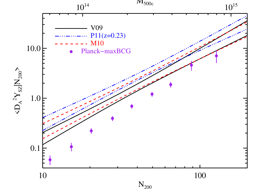
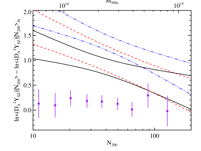
Figure 1.— Top panel: Comparison of the predicted $\left\langle Y_{\rm SZ}|N_{200}\right\rangle$ relation for each of the data sets considered in this work (V09, M10, P11) to the Planck Collaboration (P11-opt, 2011c) data, as labelled. All bands cover the 68% confidence regions for each individual scaling relation. The miscentering corrections of Biesiadzinski et al. (2012) have been applied on the data drawn from P11-opt. We have also applied the aperture-induced Malmquist bias corrections (see text). Bottom Panel: As top panel, but after subtracting the $\left\langle Y_{\rm SZ}|N_{200}\right\rangle$ fit from P11-opt. The data points do not scatter about zero because of the corrections applied. We emphasize that the uncertainty in the model predictions are strongly correlated, so $\chi^{2}$-by-eye is grossly misleading. For instance, lowering the predicted amplitude for the V09 model by $\approx 3\sigma$ results in good agreement with the data, reflecting the fact that the tension between the P11-opt data and the V09 model is only $2.8\sigma$.

3.2. Results

The top panel in Figure 1 compares the $Y_{\rm SZ}$–$N_{200}$ relation predicted using the V09, M10, and P11(z=0.23) scaling relations to the P11-opt data. Note in Figure 1 we plot $\ln\left\langle D_{A}^{2}Y_{\rm SZ}|N_{200}\right\rangle$ rather than $\left\langle\ln D_{A}^{2}Y_{\rm SZ}|N_{200}\right\rangle$ to match the P11-opt data. The bottom panel shows this same data after subtracting the $\left\langle Y_{\rm SZ}|N_{200}\right\rangle$ fit reported in P11-opt (the points do not scatter about zero because of the miscentering and aperture-induced bias corrections applied). There is reasonable agreement between the Planck–maxBCG data and the V09 and M10 models at high masses ($M\gtrsim 5\times 10^{14}\ M_{\odot}$), but all scaling relation predictions fail at low masses. Note that because the pivot point of the predicted scaling relations is $N_{200}=70$, the offset shown in Figure 1 is not simply a difference in slope: there is a significant difference in amplitude as well.

We emphasize that the uncertainty in our model predictions are comparable to or larger than the errors in the P11-opt data. Moreover, these theoretical uncertainties are very strongly correlated, so $\chi^{2}$-by-eye is grossly misleading. For instance, reducing the amplitude of our V09 model prediction by $3\sigma$ results in good agreement between the P11-opt data and our model prediction. Indeed, the tension between the V09+R09 prediction and the P11-opt data is just under $3\sigma$.

We make this quantitative by computing $\chi^{2}$, adding in quadrature the observational errors from P11-opt to the covariance matrix for the V09 predictions. We evaluate goodness of fit by generating $10^{5}$ Monte Carlo realizations of the data using the full covariance matrix, and empirically compute $P(\chi^{2}\geq\chi^{2}_{obs})$. The corresponding probabilities for each of the three models we consider are $P=0.005$ ($2.8\sigma$, V09), $P\leq 10^{-5}$ ($\gtrsim 4.4\sigma$,P11(z=0.23)), and $P=0.06$ ($1.9\sigma$, M10). Evidently, the tension is not anywhere nearly as strong as it appears by eye, though the P11(z=0.23) model is ruled out at high significance. If we used only the diagonal terms in the full covariance matrix, we find $\chi^{2}_{diag}=71$, which demonstrates how grossly misleading “$\chi^{2}$-by-eye” estimates can be.

Reconciling the $Y_{\rm SZ}$–$N_{200}$ data with our predictions requires that at least one of the input scaling relations that were used in our predictions be incorrect. R09 allows for a $10\%$ systematic error offset in the weak lensing masses used to construct the $M$–$N_{200}$ relation, but lowering the cluster masses by said amount is not sufficient to remove the tension from the data. If R09 have not underestimated their systematic uncertainty, the remaining discrepancy would have to be in the X-ray mass estimates. Because all X-ray works relied on hydrostatic mass calibration, the most obvious source of bias is non-thermal pressure support in galaxy clusters. We consider a fiducial model in which there is $15\%$ hydrostatic bias, meaning hydrostatic masses are $15\%$ lower than the true cluster masses when compared at a fixed aperture. This value is typical of what is predicted from numerical simulations ($\approx 10\%-25\%$, e.g. Nagai et al. 2007; Lau et al. 2009; Battaglia et al. 2011; Nelson et al. 2011; Rasia et al. 2012).

Because cluster masses are defined using a constant overdensity criteria, the bias between the true and reported $M_{500}$ values is larger than the mass bias at fixed aperture. For an NFW (Navarro et al. 1996) profile with $R_{500}/R_{s}=3$ (e.g. Vikhlinin et al. 2006), we find $M(R)\propto R^{0.88}$ at $R=R_{500}$. Assuming $M_{obs}(R)=bM_{true}(R)$, and expanding in a power-law around $R_{500}$, we find that the bias in the reported $M_{500}$ mass is $M_{500}^{obs}/M_{500}^{true}=b^{1.4}$, or 21% in our case. This, then, is the total mass bias we ascribe to the X-ray masses.

The top-left panel in Figure 2 compares the predicted scaling relations with the P11-opt data after including these two corrections, i.e. lowering the masses of R09 by 10% while raising X-ray masses by 21%. Possible origins of the 10% downwards shift of the maxBCG masses relative to R09 will be discussed in section 8. For the time being, we just wish to investigate whether the scaling relations modified in this way provide a good description of the data. As shown in Figure 2, the V09 and M10 models result in excellent fits to the data, with $P(\chi^{2}\geq\chi^{2}_{obs})=0.83$ and $0.52$ respectively. The P11(z=0.23) model has $P(\chi^{2}\geq\chi^{2}_{obs})=0.01$, and remains in tension with the data at the $2.5\sigma$ level.

We have also considered what happens if we increase the bias in either the weak lensing masses or the X-ray masses. In either case, increasing the mass bias by up to $\approx 20\%$ results in good agreement between the predicted and observed $Y_{\rm SZ}$–$N_{200}$ relations. Note, however, that the absence of any is ruled out. Consequently, we can think of the P11-opt as placing a lower limit to the hydrostatic and weak lensing bias in the data, while placing only a very weak upper limit on these biases.

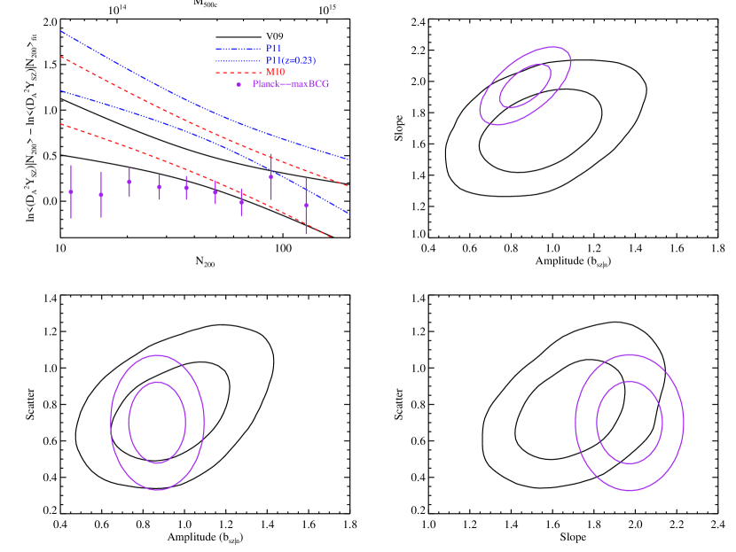
Figure 2.— Top Left: Comparison of the predicted $\left\langle Y_{\rm SZ}|N_{200}\right\rangle$ relations to the P11-opt data (corrected for miscentering and aperture–induced Malmquist bias). The prediction assumes a $15\%$ hydrostatic bias (at fixed aperture, $21\%$ total bias) in X-ray masses, and reduced the Rozo et al. (2009a) mass normalization by its allotted systematic uncertainty (10%). With these corrections, the V09 and M10 models are in good agreement with the data. Remaining panels: 68% and 95% confidence contours for the observed (purple curves) and predicted (solid curves) $Y_{\rm SZ}$–$N_{200}$ scaling relation parameters. The $Y_{\rm SZ}$–$N_{200}$ prediction focuses on the V09 model only.

We again emphasize that $\chi^{2}$-by-eye can be very misleading, and that a better sense of the agreement or tension between the P11-opt data and our predictions can be obtained by comparing the observed amplitude, slope, and scatter of the $Y_{\rm SZ}$–$N_{200}$ relation to our predictions. This comparison is shown in the remaining panels of Figure 2. We focus on the V09 measurements alone to avoid overcrowding the figure. We take $\sigma_{sz|n}=0.7\pm 0.15$ as the scatter value from P11-opt, which is broadly consistent with their Figure 4 across a large richness range. For this comparison, we have refitted the P11-opt data after miscentering corrections. We note that the amplitude parameter plotted is $\tilde{a}_{sz|n}$ rather than $a_{sz|n}$, so as to match the P11-opt data. There is good agreement between the predicted amplitude, slope, and scatter of the $Y_{\rm SZ}$–$N_{200}$ relation, with significant overlap between the two distributions. Because there is covariance between the amplitude and slope of our predicted relation, $\tilde{a}_{sz|n}$ and $\alpha_{sz|n}$ are correlated despite the fact that we chose our pivot point to decorrelate $a_{sz|n}$ and $\alpha_{sz|n}$.

3.3. The MCXC sub-sample of maxBCG Clusters

One question that we have not yet addressed is that of the SZ signal of the MCXC subsample of maxBCG galaxy clusters. P11-opt find that when they stack the sub-sample of maxBCG galaxy clusters that are also in the MCXC catalog (Piffaretti et al. 2011) — a heterogeneous compilation of X-ray selected cluster catalogs — then the observed $Y_{\rm SZ}$ signal is boosted by a large amount, and appears to be in reasonable agreement with the P11-opt predicted scaling relation. The fact that the SZ signal for the maxBCG–MCXC cluster subsample is higher than that of the full maxBCG sample has already been quantitatively addressed by Biesiadzinski et al. (2012) and Angulo et al. (2012). Consequently, we do not see a need for us to repeat their calculations here.

We would like, however, to present a simple qualitative argument that addresses these results. As noted in Rozo et al. (2009a), the scatter in mass and $L_{\rm X}$ at fixed richness are very strongly correlated ($r\geq 0.85$ at 95% CL). This reflects that fact that the maxBCG richness estimator is very noisy, much noisier than $L_{\rm X}$. Consequently, at fixed richness, a brighter cluster is always more massive. By the same token, a brighter X-ray cluster will also have a higher $Y_{\rm SZ}$ signal. Given a richness bin, a selection of the X-ray brightest clusters in the bin necessarily “peels off” the high SZ tail of the clusters in the bin. Hence, the SZ signal of the X-ray bright maxBCG sub-sample is higher than that of the full sample, as observed. Moreover, as one goes lower and lower in richness, a given luminosity cut will peel off systems that are further out in the tail of the mass distribution. That is, the lower the richness bin, the stronger the impact that the X-ray selection has on the recovered signal, in agreement with the P11-opt data.

Thus, we believe the apparent agreement between the prediction in P11-opt and the MCXC–maxBCG sub-sample of galaxy clusters is entirely fortuitous. It is clear that the strong covariance in $L_{\rm X}$ and $Y_{\rm SZ}$ at fixed richness predicts an increase in the SZ amplitude, and a flattening of the slope for the X-ray bright subsample. Since the full sample starts below the P11-opt prediction, the X-ray selection necessarily improves agreement with the model. This, however, is a selection effect that happens to move us towards the model prediction, rather than the result of a self-consistent model of cluster scaling relations. Indeed, the P11-opt prediction is explicitly a prediction for the full maxBCG sample, not for an X-ray bright sub-sample. Once one accounts for selection effects, the model curve for the MCXC–maxBCG cluster sub-sample in P11-opt would move upwards by the same amount that the P11-opt data did, preserving the original tension.

In short, the big puzzle presented by the P11-opt data is not the apparent agreement between the P11-opt model and the MCXC–maxBCG cluster sample — that is simply a fortuitous coincidence— the question is why did the model fail in the first place.

3.4. The Bigger Picture

From Figure 2, we see that the V09 model comes closest to the P11-obs data. In the interest of brevity, we will henceforth focus exclusively on the V09 model. The results from papers I and II allow us to quickly infer how the M10 and P11(z=0.23) models will behave: M10 generically agrees with V09 at high masses, but extrapolates poorly to low masses due to the constant $f_{gas}$ assumption, while the P11(z=0.23) masses are biased low by $\approx 20\%$ relative to V09 across the observed range.

Having restricted ourselves to the V09 model, we have shown that a 10% overestimate of the optical masses, and a 15% hydrostatic bias (at fixed aperture, 21% total bias) results in excellent agreement with the data. To take this solution seriously, however, these mass calibration offsets need not only explain the $Y_{\rm SZ}$–$N_{200}$ data, they must also be able to fit all multi-wavelength data available.

For the remainder of this work, we consider whether these bias-corrected V09 and R09 scaling relations can satisfy this requirement. More specifically, for our model to be successful it must satisfy the following conditions:

1. Both optical and X-ray cluster spatial abundances must be consistent with cosmological expectations in a WMAP7 cosmology.

2. Optical and X-ray spatial abundances must be consistent with each other.

3. The model must fit all scaling relation data, from both optical, X-ray, and SZ selected cluster catalogs.

4. We must be able to self-consistently use two observed scaling relations to predict a third, and the predictions must agree with observations.

We now turn to address each of these points in turn.

4. spatial abundance Constraints

In paper II, we considered the cosmological consistency of the V09 $L_{\rm X}$–$M$ scaling relation. Specifically, we showed that by convolving the $L_{\rm X}$–$M$ relation of V09 with the halo mass function (Tinker et al. 2008) in a WMAP7+BAO+$H_{0}$ (Komatsu et al. 2011) or a WMAP7+BOSS (Sanchez et al. 2012) cosmology, we can succesfully reproduce the observed REFLEX luminosity function (Böhringer et al. 2002). An obvious question that arises is whether the bias-corrected V09 scaling relation is still consistent with cosmological expectations. Moreover, one must also demand that the spatial abundance of X-ray galaxy clusters be consistent with the spatial abundance of optical galaxy clusters. That is, convolving $n(N_{200})$ with $P(L_{X}|N_{200})$ one should recover the X-ray luminosity function. We now test both of these conditions.

To estimate the X-ray luminosity function from maxBCG data, we randomly sample the $L_{\rm X}$–$N_{200}$ relation parameters (including scatter) from Rozo et al. (2009a), and use these to randomly assign an X-ray luminosity to every cluster. We then construct the cumulative luminosity function $n(L_{\rm X})$ by dividing the recovered spatial abundance by the volume sampled by the maxBCG catalog. The whole procedure is iterated $10^{4}$ times, and we compute the average cumulative luminosity function along with the corresponding uncertainty, defined as the standard deviation of our Monte Carlo analysis. We also correct the luminosity function for the expected evolution between $z=0.08$, the median redshift of the REFLEX sample, and $z=0.23$, the median redshift of the maxBCG sample, though we find this evolution is negligible for our purposes.

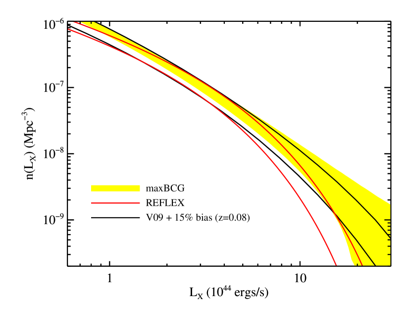
Figure 3.— Comparison of the X-ray luminosity function predicted from the maxBCG data (yellow band) to the REFLEX luminosity function (red band) (Böhringer et al. 2002), and the prediction obtained by convolving the Tinker et al. (2008) mass function and the bias-corrected V09 $L_{\rm X}$–$M$ scaling relation (black band). That is, we assume hydrostatic X-ray masses suffer from a 15% bias at fixed aperture (21% total bias). The cosmological model for the V09 prediction is a flat $\Lambda$CDM cosmology as constrained by WMAP7+BOSS (Sanchez et al. 2012). We emphasize that the yellow band from maxBCG data is completely independent of mass calibration uncertainties, and relies only on the maxBCG abundance and the $L_{X}$–$N_{200}$ scaling relation.

Figure 3 shows the maxBCG luminosity function as a yellow band. Also shown are the REFLEX luminosity function (red lines) and the V09 prediction (black solid lines) for $z=0.08$ using the bias-corrected scaling relation and the WMAP7+BOSS cosmological constraint $\sigma_{8}\Omega_{m}^{1/2}=0.441\pm 0.013$ (Sanchez, private communication, based on Sanchez et al. 2012). All three luminosity functions are in excellent agreement, with all relative offsets being significant at less than $0.3\sigma$. In principle, we should sample all cosmological parameters, but because the full covariance matrix of the cosmological parameters in Sanchez et al. (2012) is not yet publicly available, we limited ourselves to sampling only the combination $\sigma_{8}\Omega_{m}^{1/2}$. We note, however, that when using the WMAP7+BAO+$H_{0}$ chains of Komatsu et al. (2011), we find that varying all cosmological parameters or only $\sigma_{8}\Omega_{m}^{1/2}$ yields very similar results, as expected (see e.g. the discussions in Weinberg et al. 2012).

We can also directly test whether the maxBCG function and the $M$–$N_{200}$ relation from R09 are consistent with cosmological expectations. We randomly draw the parameters of the $M$–$N_{200}$ relations from Table 2, and use the resulting $P(M|N_{200})$ distribution to randomly assign masses to each maxBCG galaxy cluster. Knowing the volume sampled by the maxBCG systems ($z\in[0.1,0.3]$, $7398\ \deg^{2}$), we compute the corresponding cumulative mass function, and compare it to predictions from the Tinker et al. (2008) mass function, sampled over the cosmological constraints from Sanchez et al. (2012). As above, we sample only $\sigma_{8}\Omega_{M}^{1/2}$, holding the remaining cosmological parameters fixed. The whole procedure is iterated $10^{3}$ times, and the mean and variance of the difference between the two mass functions is stored along a grid of masses. The 68% confidence band is estimated using the $\pm\sigma$ region where $\sigma$ is the measured standard deviation.

Figure 4.— Comparison of the mass function predicted from the maxBCG data to the Tinker et al. (2008) mass function for a flat $\Lambda$CDM cosmology as constrained by WMAP+BOSS (Sanchez et al. 2012). Lowering the maxBCG masses by 10% is consistent with cosmological expectations. A 20% shift, however, starts to be in mild ($2\sigma$) tension with the data. Thus, we take this as roughly the maximum correction compatible with the Sanchez et al. (2012) results.

Figure 4 shows the difference between the cluster and halo mass functions, in units of the Poisson error. The statistical error in the spatial abundance is super-Poisson (Hu & Kravtsov 2003), but the uncertainty in the difference is actually dominated by uncertainties in cluster masses rather than cluster statistics (e.g Weinberg et al. 2012). The yellow band in Figure 4 shows the $68\%$ confidence contours for our fiducial case. The fact that this band covers the line $y=0$ demonstrates that the fiducial Rozo et al. (2009a) $M$–$N_{200}$ relation and the maxBCG spatial abundance function are consistent with cosmological expectations. The up-turn at low masses marks the scale at which the maxBCG catalog becomes incomplete.

The red dashed lines in Figure 4 shows the 68% confidence contours for the difference between the cluster and halo mass functions after reducing the amplitude of the Rozo et al. (2009a) $M$–$N_{200}$ relation by 10%. The difference between the resulting maxBCG data and the theoretical mass functions is $\approx 1.4\sigma$, so this shift in cluster masses is statistically allowed. Lowering the amplitude by 20% — shown as the green dashed–dotted curves — results in a marginally unacceptable fit, with $2.2\sigma$ tension. Thus, a $20\%$ bias on the weak lensing mass scale from R09 is roughly the maximum level of bias allowed from a cosmological perspective.

By the same token, one may ask what level of hydrostatic bias does the X-ray data allow, in the sense that the predicted and observed X-ray luminosity functions must be consistent with each other. We find that up to a $\approx 30\%$ hydrostatic bias at fixed aperture ($\approx 40\%$ total) is acceptable ($\lesssim 2\sigma$) when using WMAP7+BOSS priors. These results are entirely consistent with the biases required to explain the $Y_{\rm SZ}$–$N_{200}$ relation, i.e. 10% bias in the maxBCG masses, and a $15\%$ hydrostatic bias in X-ray masses. Interestingly, this also demonstrates that cosmological considerations can place an upper limit for the hydrostatic and weak lensing biases in the data. In conjunction with the lower limit placed by the $Y_{\rm SZ}$–$N_{200}$ relation, these limits nicely bracket our proposed solution.

5. Optical and X-ray Consistency

V09 calibrated the $L_{\rm X}$–$M$ scaling relation, as well as the $M$–$Y_{X}$ scaling relations. Using the $Y_{\rm SZ}$–$Y_{X}$ scaling relation from Rozo et al. (2012a), in paper II we used this data to also produce a V09 $Y_{\rm SZ}$–$M$ scaling relation. We now derive the $L_{\rm X}$–$M$ and $Y_{\rm SZ}$–$M$ relations from maxBCG data, and compare them to the V09 results.

5.1. Method

We rely on a Monte Carlo method to compute the scaling relations predicted from maxBCG. Specifically, we use the $M$–$N_{200}$, $L_{\rm X}$–$N_{200}$, $Y_{\rm SZ}$–$N_{200}$ scaling relations to randomly assign masses, X-ray luminosities, and SZ signals to each maxBCG galaxy cluster. We then select a mass-limited cluster sub-sample with $M\geq 2\times 10^{14}\ M_{\odot}$ — comfortably above the completeness limit of the sample, see Figure 4 — and we fit for the resulting scaling relation parameters. The whole procedure is iterated $10^{4}$ times. Each scaling relation is then evaluated along a grid in mass, and the mean and standard deviation at each point computed. The 68% confidence intervals are estimated as the $\pm\sigma$ regions where $\sigma$ is the standard deviation.

There is one additional key consideration when predicting the scaling relations from the maxBCG data: the cluster variables $L_{\rm X}$, $Y_{\rm SZ}$, and $M$, are all tightly correlated with each other at fixed richness (R09; Stanek et al. 2010; White et al. 2010; Angulo et al. 2012; Noh & Cohn 2012). This reflects the fact that $N_{200}$ is a very poor mass tracer with very large scatter: a cluster that is brighter in X-rays will also be more massive and have a higher SZ signal. We set the correlation coefficient between the various observables using the local power-law multi-variate scaling relations model detailed in Appendix A of paper II. Specifically, the covariance between a quantity $\psi$ and $m$ at fixed richness (subscript $n$) is given by

$$r_{\psi,m|n}=\frac{\sigma_{m|n}/\sigma_{m|\psi}-r}{\left[1-r^{2}+(\sigma_{m|n}/\sigma_{m|\psi}-r)^{2}\right]^{1/2}}$$ (9)

where $r$ is the correlation coefficient between $x$ and $n$ at fixed $m$. We take the simplifying assumption that this intrinsic covariance is zero ($r=0$), which implies $r_{x,m|n}=0.90$ and $r_{sz,m|n}=0.98$. Since the mass scatter at fixed optical richness ($\sigma_{m|n}$) is significantly larger its counterpart at fixed X-ray luminosity ($\sigma_{m|x}$), the precise value of $r$ has only a mild impact; varying $r\in[-0.5,0.5]$ varies $r_{x,m|n}$ over the range $r_{x,m|n}\in[0.86,0.93]$, with even a smaller range of variation for $r_{sz,m|n}$.

Equation (9) specifies the correlation coefficient we employ when assigning cluster properties to the maxBCG galaxy clusters. When evaluating the correlation coefficient, we hold the scatter $\sigma_{m|x}$ fixed to its central value. This is because the main source of scatter in $r_{x,m|n}$ is the uncertainty in $\sigma_{m|n}$. In addition, it avoids introducing covariance between fluctuations in the scaling relation predicted from maxBCG data and the V09 predictions. Because $\sigma_{m|n}$ is drawn for each Monte Carlo realization, each realization has an independent $r_{x,m|n}$ and $r_{sz,m|n}$ estimate.

To compute the 68% confidence regions for the V09 scaling relations, we rely instead on the method used in paper II: the scaling relations parameters are randomly sampled $10^{5}$ times from the priors in Tables 2 and 3. These are used to compute the scaling relation parameters using Appendix A in paper II, which we in turn us to evaluate the mean and standard deviation of the scaling relations along a grid of masses. The 68% confidence intervals are estimated as above. In all cases, the biased-corrected scaling relations are computed by modifying the amplitude of the bias-free scaling relations involving mass by the appropriate amounts (10% for R09, 21% for V09). We also rescale cluster observables defined within $R_{500}$ as in papers I and II to account for the change in aperture due to mass rescaling, though we note these corrections are typically small relative to the impact of the mass offset.

Table 3Input Scaling Relations at $z=0.23$

Relation	$\chi_{0}$	$a_{\psi|\chi}$	$\alpha$	$\sigma_{\ln\psi|\chi}$	Sample
$L_{\rm X}$–$M$	4.8	$1.16\pm 0.09$	$1.61\pm 0.14$	$0.40\pm 0.04$	V09
$D_{A}^{2}Y_{\rm SZ}$–$N_{200}$	40.0	$-0.20\pm 0.13$	$1.95\pm 0.07$	$0.70\pm 0.15$	maxBCG
$L_{\rm X}$–$N_{200}$	40.0	$0.04\pm 0.04\ (ran)$	$1.63\pm 0.06\ (ran)$	$0.83\pm 0.03\ (ran)$	maxBCG
		$~{}~{}~{}~{}~{}~{}\pm 0.09\ (sys)$	$~{}~{}~{}~{}~{}~{}\pm 0.05\ (sys)$	$~{}~{}~{}~{}~{}~{}\pm 0.10\ (sys)$

5.2. Results

Figure 5.— Top-left panel: 68% confidence interval for the $L_{\rm X}$–$M$ scaling relation at $z=0.23$ as estimated from the maxBCG catalog and V09 data sets. Both sets of scaling relations are bias-corrected, assuming a 10% overestimate of the maxBCG masses, and a 15% hydrostatic bias (at fixed aperture, 21% total bias) on the X-ray masses. Remaining panels: 68% and 95% confidence regions of the $L_{\rm X}$–$M$ parameter for the bias-corrected maxBCG (filled contours) and V09 (solid black curves) data sets. The amplitude parameter is defined at the pivot point $M=3\times 10^{14}\ M_{\odot}$, which is appropriate for the bias-corrected maxBCG data set.

The top-left panel in Figure 5 shows the 68% confidence contours for the V09 and maxBCG $L_{\rm X}$–$M$ scaling relation. Both sets of relations are bias-corrected, and are in excellent agreement with each other. The scatter, too, is in good agreement, with $\sigma_{\ln L_{\rm X}|M}=0.38^{+0.10}_{-0.05}$ for the maxBCG prediction, and $\sigma_{\ln L_{\rm X}|M}=0.40\pm 0.04$ for the V09 scaling relation. This agreement is better illustrated in the remaining panels, where we explicitly compare the predicted amplitude, slope, and scatter of the $L_{\rm X}$–$M$ relation from the two works. In all cases, the filled contours correspond to the maxBCG bias-corrected scaling relations, while the solid curves demarcate the bias-corrected V09 scaling relation.

Figure 6 mirrors Figure 5, only there we are considering the $Y_{\rm SZ}$–$M$ scaling relations. The top-left panel shows the 68% confidence interval in the $Y_{\rm SZ}$–$M$ plane, while the remaining panels show the 68% and 95% confidence contours for the scaling relation parameters. In all cases, we consider only the bias-corrected scaling relations. Even though the agreement is less good than in the case of the $L_{\rm X}$–$M$ relation, the agreement between the two data sets is still adequate.

Despite the two data sets being in statistical agreement, it is worth asking what would be required to improve upon the current status, particularly in the case of $Y_{\rm SZ}$–$M$, where the agreement is less good. Because the maxBCG band falls below the V09 data in the $Y_{\rm SZ}$–$M$ plane, but above the V09 data in the $L_{\rm X}$–$M$ plane, shifting the cluster masses will increase tension in one relation while alleviating the other, and is therefore not a good avenue for improving things. In addition, the X-ray luminosities are tied down by the spatial abundance constraints from the previous section. Consequently, any improvement to the current scenario would have to come from $\approx 10\%-20\%$ changes in the $Y_{\rm SZ}$ measurements: either the V09 $Y_{\rm SZ}$ measurements would have to go down (e.g. due to Malmquist bias due to SZ cluster selection), or the P11-opt measurements would have to go up. Since the V09 $Y_{\rm SZ}/Y_{X}$ ratio is already on the low end of what is expected, an increase of the $Y_{\rm SZ}$ signal of maxBCG clusters is the most promising avenue.

If we repeat this analysis using the original maxBCG and V09 scaling relations, we find that while the two data sets are in modest agreement with regards to the $L_{\rm X}$–$M$ relation, the $Y_{\rm SZ}$–$M$ relation of the two works are clearly discrepant. This disagreement reflects the original tension in the $Y_{\rm SZ}$–$N_{200}$ relation, so it is not surprising that fixing the $Y_{\rm SZ}$–$N_{200}$ relation also results in consistent estimates for the $Y_{\rm SZ}$–$M$ relation. That said, it is far from trivial that this same solution is consistent with the $L_{\rm X}$–$M$ relation, and with the spatial abundance constraints discussed in the previous section.

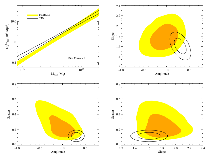
Figure 6.— Top-left panel: 68% confidence interval for the $Y_{\rm SZ}$–$M$ scaling relation at $z=0.23$ as estimated from the maxBCG catalog and V09 data sets. Both sets of scaling relations are bias-corrected, assuming a 10% overestimate of the maxBCG masses, and a 15% hydrostatic bias (at fixed aperture, 21% total bias) on the X-ray masses. Remaining panels: 68% and 95% confidence regions of the $Y_{\rm SZ}$–$M$ parameter for the bias-corrected maxBCG (filled contours) and V09 (solid black curves) data sets. The amplitude parameter is defined at the pivot point $M=3\times 10^{14}\ M_{\odot}$, which is appropriate for the bias-corrected maxBCG data set.

6. Closure Test: the $Y_{\rm SZ}$–$L_{\rm X}$ Relation

We have seen that the bias-corrected $L_{\rm X}$–$M$ and $Y_{\rm SZ}$–$M$ maxBCG and V09 scaling relations are in good agreement with each other, and are also consistent with cosmological expectations. We now test whether the direct observable scaling relations are self-consistent. Specifically, we test whether the $Y_{\rm SZ}$–$L_{\rm X}$ relation predicted from the $Y_{\rm SZ}$–$N_{200}$ and $L_{\rm X}$–$N_{200}$ relations is consistent with measurements from X-ray cluster catalogs. Further, we will also compare the predicted $Y_{\rm SZ}$–$L_{\rm X}$ scaling relations to the bias-corrected prediction from the V09 model.

The maxBCG predictions are computed as before: we randomly assigned $L_{\rm X}$ and $Y_{\rm SZ}$ values to clusters in the catalog, including the effect of the correlation coefficient. The correlation coefficient between $Y_{\rm SZ}$ and $L_{\rm X}$ at fixed richness is estimated following an argument similar to the previous section. Specifically, we assume $r_{n,x|sz}=0$, and estimate $r_{x,sz|n}$ using the formulae in Appendix A of paper II. Typical values for $r_{x,sz|n}$ lie in the range $[0.8,1]$, as expected. We then cut the resulting cluster catalog at $L_{\rm X}\geq 8\times 10^{43}\ \mbox{ergs/z}$, which is sufficiently high to not be affected by completeness issues, and fit the data to arrive at our model amplitude, slope, and scatter about the mean. The V09 predictions are performed exactly as in paper II, where we also considered the $Y_{\rm SZ}$–$L_{\rm X}$ relation for the V09, M10, and P11 data sets, only we now consider the bias-corrected V09 scaling relations only.

Figure 7.— Top-left panel: 68% confidence interval for the $Y_{\rm SZ}$–$M$ scaling relation at $z=0.23$ as estimated from the maxBCG catalog (yellow band) and V09 (black lines) data sets. Both sets of scaling relations are bias-corrected, assuming a 10% overestimate of the maxBCG masses, and a 15% hydrostatic bias (at fixed aperture, 21% total bias) on the X-ray masses. Also shown as a purple band is the 68% confidence interval quoted in Planck Collaboration (2011a) from stacking X-ray selected clusters from the MCXC catalog (Piffaretti et al. 2011). We have corrected these fits for Malmquist bias due to correlated scatter, and aperture corrections due to the mass bias relative to V09 (see text). The green line is our own fit to the P11(z=0.23) data, modified for selection effects as described in P11. The data points with error bars are clusters with $z\in[0.13,0.3]$ in P11. Blue points are cool-core systems, while red points are not. The green line is the best fit relation to the P11(z=0.23) data. Remaining panels: 68% and 95% confidence regions of the $Y_{\rm SZ}$–$M$ parameter for the bias-corrected maxBCG (yellow contours) and V09 (solid black curves) data sets. The amplitude parameter is defined at a pivot point $L_{\rm X}=2\times 10^{44}\ \mbox{ergs/s}$, which is a compromise between the V09 and maxBCG predictions. The green contours corresponds to our fit of the P11 data, while the purple contours are those obtained from the MCXC catalog.

We will be comparing the maxBCG and V09 predictions for the $Y_{\rm SZ}$–$L_{\rm X}$ scaling relation to those derived from the P11(z=0.23) data, and that obtained by stacking X-ray galaxy clusters from the MCXC cluster catalog (Piffaretti et al. 2011) as described in Planck Collaboration (2011a), hencerforth referred to as P11-X. For the P11(z=0.23) data, we fit the clusters in P11 in the redshift range $z\in[0.13,0.3]$, and modify the recovered amplitude as described in P11. We do not attempt to measure the scatter because of selection effects. Rather, our fits assume an intrinsic scatter in $Y_{\rm SZ}$–$L_{\rm X}$ of $0.4$, which is consistent with all data.

As for the P11-X fits to the $Y_{\rm SZ}$–$L_{\rm X}$ scaling relation, we perform three independent corrections: 1) Malmquist bias corrections due two covariance between $Y_{\rm SZ}$ and $L_{\rm X}$. 2) Aperture induced corrections due to the difference in mass calibration between P11 and the bias-corrected V09 model. 3) A correction to account for the fact that P11-X measure $\left\langle Y_{\rm SZ}|L_{\rm X}\right\rangle$ rather than $\left\langle\ln Y_{\rm SZ}|L_{\rm X}\right\rangle$.

The first of these corrections — the Malmquist bias due to correlated scatter — works exactly as per our discussion of the $Y_{\rm SZ}$–$N_{200}$ scaling relation, with an additional important consideration: in addition to aperture-induced covariance, $Y_{\rm SZ}$ and $L_{\rm X}$ are expected to be correlated because they probe the same intra-cluster medium. The correlation coefficients predicted in Stanek et al. (2010) and Angulo et al. (2012) are $r\approx 0.8$ and $r\approx 0.5$ respectively. We set $r_{sz,x|m}=0.65\pm 0.2$, where the uncertainty in $r$ is propagated into the uncertainty of the amplitude of the $Y_{\rm SZ}$–$L_{\rm X}$ relation. We also use the scatter estimates for $\sigma_{sz|m}$ and $\sigma_{x|m}$ from the V09 model, and propagate the associated uncertainty. The net effect of this correction is to lower the $Y_{\rm SZ}$ amplitude by $\approx 7\%\pm 2.5\%$.

The aperture correction to the P11-X data has to do with the dependence of $Y_{\rm SZ}$ on the integration aperture $R_{500}$. From paper 1, we know that a bias $b_{m}$ in the mass induces an amplitude shift $\Delta a=0.27\ln b_{m}$ on $Y_{\rm SZ}$. The P11(z=0.23) masses are biased by $\Delta\ln M\approx 0.2$ relative to V09, which itself suffers from a $15\%$ hydrostatic bias in our bias-corrected model. All told, this increases the $Y_{\rm SZ}$ amplitude by $\approx 10\%\pm 3\%$.

Finally, the cluster stacks in P11-X measure $\left\langle Y_{\rm SZ}|L_{\rm X}\right\rangle$ rather than $\left\langle\ln Y_{\rm SZ}|L_{\rm X}\right\rangle$, so their reported amplitude must be lowered accordingly, by $\approx 8\%\pm 2\%$. Put together, these three corrections result in an amplitude shift of $\Delta a_{sz|x}=-0.050\pm 0.044$. We apply this systematic correction to the P11-X data, and add the associated uncertainty in quadrature to their quoted errors.

The top-left panel in Figure 7 compares the predicted $Y_{\rm SZ}$–$L_{\rm X}$ scaling relation derived from the V09 data set (black solid lines) with that of the maxBCG catalog (yellow band). Note for both of these, we only consider the bias-corrected scaling relations (mass enters via the aperture corrections to $Y_{\rm SZ}$). The purple band is the observed relation in the MCXC cluster catalog from P11-X. The best fit line to the P11(z=0.23) data set is shown as a solid green line. The points with error bars are individual clusters in the P11(z=0.23) data set, blue for cool-core systems, and red for non cool-core systems.

The agreement between the various data sets is best judged using the remaining panels of Figure 7, where we show the corresponding 68% and 95% confidence contours for the scaling relation parameters. Focusing on the top-right plot, which shows the amplitude and slope parameters, we see that the P11(z=0.23) data is in some tension with the other data sets: the amplitude is too high. The simplest explanation for this offset would be an underestimate of the SZ selection effects in P11.

There is, however, reasonable agreement between the maxBCG, V09, and P11-X data sets: the $1\sigma$ P11-X data curve in the top-right panel overlaps the $1\sigma$ contours for both the maxBCG and V09 data sets. All three data sets are in excellent agreement on the intrinsic scatter in the $Y_{\rm SZ}$–$L_{\rm X}$ relation. To achieve better agreement, the $Y_{\rm SZ}$ signal of the maxBCG galaxy clusters would need to increase by $\approx 10\%-20\%$, especially at low masses; a decrease of the V09 $Y_{\rm SZ}$ signal would be difficult to reconcile with X-ray expectations for the $Y_{\rm SZ}/Y_{X}$ ratio, while shifts of the X-ray luminosity are limited by spatial abundance constraints.

7. The Mass Scale of Galaxy Clusters

7.1. The Mass Scale of maxBCG Galaxy Clusters

We have already argued that the origin of the bias in X-ray masses proposed in this paper is simple hydrostatic bias. One interesting question that remains open, however, is where did the bias in the stacked weak lensing mass calibration in R09 come from? At least part of this answer has to do with the impact of covariance between mass and weak lensing mass at fixed richness. Covariance between $M_{wl}$ and $N_{200}$ introduces corrections in mass calibration that were ignored in Johnston et al. (2007) and R09. Specifically, from Appendix A in paper II we have

$$\left\langle\ln M_{wl}|N_{200}\right\rangle = a_{wl|m}+\alpha_{wl|m}\left\langle\ln M|N_{200}\right\rangle$$ (10)

$$\hskip 14.45377pt+r_{wl,n|m}\beta\alpha_{wl|m}\sigma_{m|wl}\sigma_{m|n}$$

where we have assumed

$$\left\langle\ln M_{wl}|M\right\rangle=a_{wl|m}+\alpha_{wl|m}\ln M.$$ (11)

Assuming the weak lensing mass estimates are unbiased in the sense that $\left\langle\ln M_{wl}|M\right\rangle=\ln M$, we can set $a_{wl|m}=0$ and $\alpha_{wl|m}=1$. Inserting this into our expression for $\left\langle\ln M_{wl}|N_{200}\right\rangle$, and solving for $\left\langle\ln M|N_{200}\right\rangle$ we find

$$\left\langle\ln M|N_{200}\right\rangle=\left\langle\ln M_{wl}|N_{200}\right\rangle-r_{wl,n|m}\beta\sigma_{m|wl}\sigma_{m|n}$$ (12)

Table 4Preferred Set of Scaling Relations

Relation	$\chi_{0}$	Amplitude ($a_{\psi|\chi}$)	$\alpha_{\psi|\chi}$	$\sigma_{\ln\psi|\chi}$	Sample
$L_{\rm X}$–$M$	4.4	$0.72\pm 0.07\ (ran)\pm 0.16\ (sys)$	$1.55\pm 0.09$	$0.39\pm 0.03$	V09+maxBCG
$D_{A}^{2}Y_{\rm SZ}$–$M$	4.4	$0.87\pm 0.06\ (ran)\pm 0.17\ (sys)$	$1.71\pm 0.08$	$0.15\pm 0.02$	V09+maxBCG
$M$–$N_{200}$	40	$0.75\pm 0.10$	$1.06\pm 0.11$	$0.45\pm 0.10$	maxBCG
$L_{\rm X}$–$N_{200}$	40	$0.04\pm 0.10$	$1.63\pm 0.08$	$0.83\pm 0.10$	maxBCG
$Y_{\rm SZ}$–$N_{200}$	40	$-0.24\pm 0.20$	$1.97\pm 0.10$	$0.70\pm 0.15$	maxBCG
$Y_{\rm SZ}$–$L_{\rm X}$	1.0	$-0.29\pm 0.06$	$1.10\pm 0.03$	$0.40\pm 0.05$	P11-X

We see then that any covariance between $M_{wl}$ and $N_{200}$ at fixed mass implies that the weak lensing masses must be corrected downwards. This is exactly the same type of Malmquist-bias correction that we applied on the $Y_{\rm SZ}$–$N_{200}$ and $Y_{\rm SZ}$–$L_{\rm X}$ scaling relations, though this covariance is not aperture-induced. In Angulo et al. (2012), the correlation coefficient $r_{wl,n|m}$ is estimated to be $r\approx 0.4$, in good agreement with the value from Noh & Cohn (2012). Assuming $\sigma_{wl|m}\approx 0.2$ as per Becker & Kravtsov (2011), $\sigma_{n|m}\approx 0.4$, and $\beta\approx 3$, and setting $r$ to the Angulo et al. (2012) value, we find that the mass calibration from R09 should be corrected downwards by $10\%$. This correction is in excellent agreement with the conclusions from our study. As in the case of the $Y_{\rm SZ}$–$N_{200}$ relation, the covariance between $M_{wl}$ and $N_{200}$ may be somewhat overestimated. For instance, Angulo et al. (2012) measured $M_{wl}$ within $\left\langle R_{500}|N_{200}\right\rangle$, whereas $M_{wl}$ in R09 comes from directly fitting a halo model to the shear data. Consequently, the Angulo et al. (2012) value likely needs to be reduced for the impact of aperture-induced covariance. However, orientation effects due to optical cluster selection does appear to induce some covariance that can lead to $\approx 6\%$ overestimates of cluster masses if this affects is unaccounted for (Jörg Dietrich, private communication), and the Noh & Cohn (2012) value for the correlation coefficient is not affected by aperture-induced covariance. Overall, it seems clear that a $\approx 10\%$ downwards correction to the R09 masses due to covariance between $M_{wl}$ and $N_{200}$ is a plausible explanation for the shift in the mass-scale of maxBCG galaxy clusters needed by our self-consistent model of multi-variate cluster scaling relations. We note, however, that such a shift is also within the systematic error allotted due to cluster miscentering and source photometric redshift errors.

In this context, it is also worth emphasizing that while much of the work addressing the P11-opt data has focused on the Johnston et al. (2007) scaling relation, this is not well justified. As was first pointed out by Mandelbaum et al. (2008b), one expects significant photometric redshift corrections relative to the raw data from Johnston et al. (2007). These correction arise because the lens and source populations in the SDSS are overlapping, which tends to dilute the weak lensing signal. Moreover, the inverse critical surface density varies quickly with source redshift when $z_{source}\approx z_{lens}$, making weak lensing masses more sensitive to photometric errors. R09 applied these corrections, and combined the corrected Sheldon et al. (2009) and Johnston et al. (2007) analysis with that of Mandelbaum et al. (2008a) to place priors on the $M$–$N_{200}$ relation of maxBCG galaxy clusters, including this effect. These corrections should be applied. Moreover, there are now several independent stacked weak lensing mass calibrations of the maxBCG galaxy clusters (Mandelbaum et al. 2008a; Simet et al. 2012; Bauer et al. 2012), all of which are consistent with the R09 scaling relation. Importantly, all these studies are also subject to the covariance-induced Malmquist bias noted above.

7.2. Preferred Set of Scaling Relations

We have demonstrated that the bias-corrected R09 and V09 cluster scaling relations are fully self-consistent; not only are the observable–mass relations derived from optical and X-ray selected cluster catalogs consistent with one another, the optical and X-ray spatial abundance functions are consistent with each other and with cosmological expectations. Because the $L_{\rm X}$–$M$ and $Y_{\rm SZ}$–$M$ scaling relations predicted from the bias-corrected maxBCG and V09 scaling relations are in good agreement with each other, we combine them to arrive at our preferred estimates for these relations. These are summarized in Table 4, along with our preferred set of scaling relations for $M$–$N_{200}$, $L_{X}$–$N_{200}$, $Y_{\rm SZ}$–$N_{200}$, and $Y_{\rm SZ}$–$L_{X}$. For this last set of scaling relations we do not attempt to combine the maxBCG and V09 bias corrected results: rather, we rely on the measurement that most directly probes each scaling relation. We emphasize, however, that this set of scaling relations is still fully self-consistent with the quoted uncertainties. The pivot point for $L_{X}$–$M$ and $Y_{\rm SZ}$–$M$ is set to $4.4\times 10^{14}\ M_{\odot}$ has been chosen so as to decorrelate the amplitude and slope of the joint scaling relations. We expect a conservative estimate of the systematic uncertainty due to the hydrostatic bias and weak lensing bias corrections is $10\%$ in mass, which we expect is best modeled as a top-hat distribution rather than a Gaussian. This error corresponds to a $\pm 0.16$ error in the amplitude for $L_{\rm X}$–$M$, and a $\pm 0.17$ uncertainty in the amplitude for $Y_{\rm SZ}$–$M$. We now employ our preferred set of scaling relations to predict the cluster masses for each of the CLASH systems, and to compare the masses recovered from these scaling relations to those from various works in the literature.

7.3. CLASH Predictions

Our final set of scaling relations in Table 4 fits an extra-ordinary amount of data, and satisfies a large variety of highly non-trivial internal consistency constraints. As such, we believe it can provide a critical low-redshift foundation for the study of cluster scaling relations and their evolution. In addition, these relations provide a clear target for the CLASH (Postman et al. 2012) experiment, which seeks to provide very high precision masses for a small subset of X-ray and lensing selected galaxy clusters. In Table 5, we have provided predictions for the cluster masses for each of the $z\leq 0.4$ CLASH galaxy clusters based on their X-ray luminosity, as quoted in M10. We have limited ourselves to $z\leq 0.4$ clusters to minimize the impact of redshift evolution in our scaling relations, for which we assume self-similar evolution, $L_{X}\propto E^{2}(z)$, as appropriate for soft X-ray band cluster luminosities. For the few CLASH systems not in M10, Mantz shared with us X-ray luminosities derived using the same data analysis pipeline as in M10 (Mantz, private communication). Note that to make these predictions, we utilize the distribution $P(M|L_{\rm X})$ rather than $P(L_{\rm X}|M)$. The two are related as described in Appendix A of paper II, and we have assumed a slope of the halo mass function of $\beta=4$, as appropriate for $\approx 10^{15}\ M_{\odot}$ galaxy clusters.

Unfortunately, the large scatter in the $L_{\rm X}$–$M$ relation implies that our predicted masses are highly uncertain, as there is an irreducible $\pm 25\%$ intrinsic scatter. Predictions using the SZ signal are significantly more precise, but there is only one $z\leq 0.4$ CLASH system with SZ measurements in the P11 sample, Abell 2261, which we discuss more fully below. $Y_{\rm SZ}$ estimates for these galaxy clusters is very desirable for the purposes of tightening our theoretical predictions. We also note that all of our mass predictions have an overall systematic floor of $\pm 10\%$. As emphasized in paper II, it is worth remembering that the mass estimates from scaling relations are only as good as the input data used to estimate the cluster masses. For instance, in the MCXC cluster catalog (Piffaretti et al. 2011), clusters A 383, A 209, A 1423, A 611, and MACS J1532, all have luminosities that differ from the ones quoted above by $30\%$ or more. Should these luminosities be correct, then our mass predictions would necessarily be biased by the corresponding amount.

At this time, there are only two clusters with published masses from a full-lensing analysis of CLASH data: Abell 2261 and MACS J1205-08. Our prediction for Abell 2261 is $M_{500c}=1.07\pm 0.28\ (stat)\times 10^{15}\ M_{\odot}$ based on its X-ray luminosity, and $M_{500c}=1.16\pm 0.14\ \times 10^{15}\ M_{\odot}$ based on its SZ signal (both have an additional $\pm 10\%$ top-hat systematic uncertainty). For the latter, we again assume self-similar evolution, with $Y_{\rm SZ}\propto E(z)^{2/3}$, and we have applied the expected aperture correction due to the shift in mass calibration between our work and that of P11. Coe et al. (2012) quote virial masses and concentrations rather than $M_{500c}$, so we use their best fit model to convert their numbers to $M_{500c}$. They find $M_{500c}=1.34\pm 0.13\times 10^{15}\ M_{\odot}$, in excellent agreement with either of our predictions. By comparison, the mass of A2261 in P11— which P11 obtains based on their $Y_{X}$ measurements — is $M_{500c}=0.64\pm 0.04$, is in tension with the Coe et al. (2012) value at $5\sigma$.

Turning to MACS J1205-08, our predicted masses from $L_{X}$ and $Y_{\rm SZ}$ are $M_{500c}=1.26\pm 0.34\times 10^{15}\ M_{\odot}$ and $M_{500c}=1.36\pm 0.20\times 10^{15}\ M_{\odot}$ respectively. For the $L_{X}$-based mass, we relied on the X-ray luminosity from P11. The reported mass in Umetsu et al. (2012) corresponds to $M_{500c}=1.01\pm 0.15\times 10^{15}\ M_{\odot}$, in excellent agreement with both our X-ray and SZ derived cluster mass estimates. The corresponding mass in P11 is $M_{500c}=1.08\pm 0.24$, also in good agreement with the CLASH measurement. We emphasize that the predicted uncertainties in our SZ masses are $12\%$ and $15\%$ respectively, so the agreement between our predicted masses and those from the CLASH collaboration is non-trivial. It should also be noted that Umetsu et al. (2012) find good agreement between their lensing mass estimates and direct hydrostatic mass estimates from a joint analysis of Chandra and XMM data and an independent analysis of SZ data as per Mroczkowski (2011).

Table 5$M_{500c}$ Predicted Masses for $z\leq 0.4$ CLASH Clusters

Cluster	$z$	$L_{\rm X}\ (10^{44}\ \mbox{ergs/s})$	$M_{500c}\ (10^{15}\ M_{\odot})$
A 383	0.187	5.9 $\pm$ 0.2	0.69 $\pm$ 0.18
A 209	0.206	8.6 $\pm$ 0.3	0.87 $\pm$ 0.23
A 1423	0.213	6.2 $\pm$ 0.4	0.70 $\pm$ 0.19
A 2261	0.224	12.0 $\pm$ 0.4	1.07 $\pm$ 0.28
RX J2129	0.234	9.9 $\pm$ 0.5	0.94 $\pm$ 0.25
A 611	0.288	7.5 $\pm$ 0.4	0.75 $\pm$ 0.20
MS 2137	0.313	12.3 $\pm$ 0.4	1.02 $\pm$ 0.27
MACS J1532	0.345	19.8 $\pm$ 0.7	1.36 $\pm$ 0.36
RX J2248	0.348	30.8 $\pm$ 1.6	1.80 $\pm$ 0.49
MACS J1931	0.352	19.7 $\pm$ 1.0	1.36 $\pm$ 0.36
MACS J1115	0.352	14.5 $\pm$ 0.5	1.10 $\pm$ 0.29
MACS J1720	0.391	10.2 $\pm$ 0.4	0.86 $\pm$ 0.23
MACS J0429	0.399	10.9 $\pm$ 0.6	0.89 $\pm$ 0.24

7.4. Predicted Masses for V09, M10, and P11

Just as we predicted the cluster masses for the CLASH cluster sample, we can use our best fit $L_{X}$–$M$ relation to derive cluster masses for each of the galaxy clusters in V09, M10, and P11. Our results are summarized in Figure 8, where we plot $\ln\left\langle M|L_{X}\right\rangle-\ln M_{lit}$ versus cluster redshift for each of the three cluster samples: V09 (black points), M10 (red points), and P11 (blue points). To evolve the scaling relation away from $z=0.23$, we assume a self-similar evolution $L_{X}\propto E^{2}(z)$. In deriving these masses, we use the X-ray luminosity quoted in each work.

As expected, our recovered masses are higher than those from V09: $11\%\pm 4\%$ for the low redshift sample, and $22\%\pm 5\%$ for the high redshift cluster sample. Note that our putative bias-corrected V09 scaling relation assumed a $15\%$ hydrostatic bias, which would naturally result in a $\approx 20\%$ offset. However, upon combining this scaling relation with maxBCG one, the mass scale decreases slightly, leading to the smaller low redshift bias estimated above. Turning to M10, we find that our predicted masses are in excellent agreement with theirs: the mass offset is $\Delta\ln M=2\%\pm 3\%$, and there is no evidence of evolution in the mass offset. M10 notes that a Chandra calibration update that appeared as the work was being published lowers their masses relative to the published values by $\approx 11\%$, which would result in a net offset $\Delta\ln M=13\%\pm 3\%$.

Turning to the P11 data set, for the low redshift sample ($z\leq 0.13$) we see a clear redshift trend in the data, with the mass offset increasing with increasing redshift. Whether this trend will remain as deeper data comes out remains to be seen. If we ignore this evolution and simply compute the mean mass offset, we find $\Delta\ln M=9\%\pm 6\%$. For the high redshift cluster sample ($z>0.13$), we no longer see systematic evolution in the mass offset, finding $\Delta\ln M=21\%\pm 4\%$. We warn, however, that because these clusters were also SZ-selected, the SZ selection may pick up the more massive clusters at fixed X-ray luminosity. Such a selection would tend to increase the X-ray masses from P11, thereby reducing the apparent offset relative to our mass calibration. To test for this possibility, we also computed the mass offset relative to the X-ray masses in Pratt et al. (2009), for which we find $\Delta\ln M=28\%\pm 0.05\%$.

The mass offset between our predicted masses and those of M10 and P11 are very surprising. Naively, we would have expected the sum of the offsets between our masses and those in M10 and P11 to be consistent with the M10–P11 offset, but this is not the case. That is, despite the fact that at at $z\approx 0.3$ we find that the M10 masses are higher than those in P11 by $\approx 45\%\pm 6\%$, when we look at the full M10 and P11 cluster samples, our masses are only $\approx 20\%$ higher than those in P11, and consistent with M10. The difference is due to the particular cluster sub-sample on which we based the M10–P11 comparison: for this sub-sample, our predicted masses are $18\%\pm 6\%$ lower than those in M10, and $29\%\pm 4\%$ higher than those in P11. Evidently, exactly which clusters are used for these type of comparisons can dramatically impact the conclusions we draw. One possible explanation for this difference is that the SZ selection of the P11 cluster sample implies that high-$L_{X}$, low $M_{gas}$ systems are under-represented in the P11 sample. For instance, the P11 sample may be picking out the tail of high $M_{gas}$ clusters in M10 at fixed $L_{X}$. Qualitatively, this is exactly analogous to the problem of the MCXC sub-sample of maxBCG galaxy clusters: starting from a sample selected on a noisy estimator ($L_{X}$), the interpretation of sub-samples selected using higher-quality mass proxies can be subject to important selection effects due to observable covariance. Quantitatively addressing this question, however, would require extensive simulations with covariant scatter between $L_{X}$, $Y_{\rm SZ}$, and $M_{gas}$, which is beyond the scope of this work. This does, however, illustrate that the type of naive comparisons that we are performing in this section and the next can in principle be subject to significant selection effects due to covariance between cluster observables.

Figure 8.— The mass offset $\ln\left\langle M|L_{X}\right\rangle-\ln M_{lit}$ between the expectation value of the cluster mass as per our scaling relations, and the mass quoted in V09 (black points), M10 (red points), and P11 (blue points). The lines show the mean mass for each of the various cluster sub-samples, including a low/high redshift partition of the V09 and P11 cluster samples. The length of each of the lines shows the redshift range used to define each cluster subsample. We plot a power-law model in $1+z$ whenever the best fit power-law has a non-zero slope at more than $2\sigma$ significance. Otherwise, we plot the inverse-variance weighted mean. The square with error bars in the lower left hand corner is to illustrate the typical uncertainty in the offsets, which is entirely driven by the intrinsic scatter of the $M$–$L_{X}$ relation.

7.5. Comparison to Other Weak Lensing Masses

We now perform a similar exercise to the one above, but focusing on masses derived from weak lensing analyses instead. The LoCuSS collaboration have set out to accurately calibrate cluster scaling relations by providing detailed weak lensing masses of a sample of $\approx 100$ X-ray selected galaxy clusters. Their largest compilation of weak lensing masses to date is that from Okabe et al. (2010). In a recent work, the Planck collaboration compared their X-ray derived masses to those from Okabe et al. (2010), finding that the latter are $\approx 20\%$ lower than the X-ray masses derived by the Planck team (Planck Collaboration 2012). This measurement stands in stark contrast to the solution advocated here, as we have argued that the P11 masses are too low by $\approx 20\%$.

In Figure 9, we compare our predicted masses from $L_{X}$ to those quoted in Okabe et al. (2010, red points). There is a very large offset between our predictions and their masses, $\Delta\ln M=0.53\pm 0.07$, nearly a factor of two. This value is somewhat higher than the expected offset of $\approx 0.4$ derived from the naive sum of the P11 offset relative to our predictions, and the offset quoted in Planck Collaboration (2012).

As was demonstrated in paper II, the mass calibration used by P11 results in strong ($>4\sigma$) tension between the observed X-ray luminosity function, and the cosmological expectations for a WMAP7 cosmology. Further lowering the cluster masses can only increase this tension. Should the Okabe et al. (2010) masses be correct, the X-ray luminosity function in Böhringer et al. (2004) would need to be corrected upwards by a factor of 3 to 4, implying the REFLEX catalog is $\approx 70\%$ incomplete. We find this level of incompleteness much too high to be plausible, so we expect there remains an unknown source of systematic bias in the weak lensing measurements of Okabe et al. (2010). Interestingly, Okabe et al. (2010) measured the CLASH cluster A 2261 as part of their Subaru weak lensing campaign. For this cluster, they find $M_{500c}=8.14\pm 1.17\times 10^{14}\ M_{\odot}$. This mass is indeed biased low relative to the CLASH value, with the net mass offset being $\Delta\ln M=0.50\pm 0.18$.

Figure 9.— The mass offset $\ln\left\langle M|L_{X}\right\rangle-\ln M_{lit}$ between the expectation value of the cluster mass as per our scaling relations, and the weak lensing mass quoted in Okabe et al. (2010, red points) and Mahdavi et al. (2008, black points). The lines show the inverse-variance weighted mean for each sample. The squares with error bars in the upper right hand corner illustrate the typical uncertainties in the offsets, which can be dominated by the weak lensing uncertainties.

We also compare our overall mass calibration to that of Mahdavi et al. (2008), relying on luminosity estimates from M10 to perform the comparison. This cluster sample is identical to that of Hoekstra (2007), but updated with improved photometric redshifts for source galaxies. Our results are shown in Figure 9 using black points. The mean mass offset is $\Delta\ln M=0.22\pm 0.12$, with our predicted masses being larger than those of Hoekstra (2007). Given the large uncertainties in the weak lensing masses, however, the two data sets are statistically consistent with each other.

For completeness, we have also searched for clusters in common to Mahdavi et al. (2008) and Okabe et al. (2010), finding 6 such systems. One cluster, Abell 209, might be an outlier, but it is difficult to tell with such a small sample size. The mean mass offsets with and without Abell 209 are $-0.27\pm 0.29$ and $-0.37\pm 0.18$ respectively. Note that despite the large offsets between the two works, the scatter is such that based on these 6 systems we cannot conclude that the two data sets are inconsistent with each other.

Hoekstra et al. (2011) have extended the cluster sample from Mahdavi et al. (2008) to include low mass, high redshift systems. We assume a concentration parameter $c_{500}=R_{500c}/R_{2500c}=3$ to convert their reported $M_{2500c}$ masses to $M_{500c}$, but note that our conclusions are sensitive to the assumed value of $c_{500}$. The value we adopt here is consistent with X-ray observations (e.g. Vikhlinin et al. 2006) and numerical simulations (e.g. Bhattacharya et al. 2011). A reasonable estimate for the systematic uncertainty in the mass corrections is $\pm 10\%$. With our fiducial correction, we find that the mean mass offset between the two works is $\Delta\ln M=13\%\pm 13\%$. Thus, our predicted masses are fully consistent with those in Hoekstra et al. (2011). We caution, however, that there is very large scatter in this comparison, reflecting the large errors in the weak lensing masses: 12% of the systems in that work have a reported mass that is within $1\sigma$ of zero, and a full $68\%$ of the systems are within $2\sigma$ of zero.

The final work we consider here is that of Umetsu et al. (2011), who combined magnification and shear measurements to derive constraints on five galaxy clusters: A 1689, A 1703, A 370, CL0024+17, and RXJ1347-11. The inverse variance weighted mean offset relative to our predictions (using luminosities in M10 or provided by Adam Mantz, private communication) is $\Delta\ln M=-0.42\pm 0.14$, with our predicted masses being lower. This offset reflects the fact that there are two systems with fairly large offsets: A370, with $\Delta\ln M=-0.85\pm 0.29$, and CL0024+17, with $\Delta\ln M=-1.26\pm 0.30$. The offset for CL0024+17 ($L_{X}=2.3\pm 0.1$) is so large that it is the only system we have encountered where our predicted mass was more than $3\sigma$ away from the reported mass. Both A370 and CL0024+17 are truly exceptional systems. A370 was one of the first cluster lenses ever identified (Soucail et al. 1987a, b), and may be the most massive lensing cluster in the Universe (Broadhurst et al. 2008; Umetsu et al. 2011). It also exhibits bimodality in its mass distribution, both in X-rays and lensing (Richard et al. 2010), with the two components separated in redshift by $\approx 3,000\ \mbox{km/s}$ (de Filippis et al. 2005). CL0024+17 is also known as an exceptional lensing system (Zitrin et al. 2009), and appears to be a recent cluster merger along the line of sight, leading to high weak lensing mass and a highly diffuse gas distribution (Umetsu et al. 2010). Given that these two clusters are known to be some of the most effective lenses in the Universe, and the small sample size of the cluster sample, we are loathe to derive any conclusions from this comparison.

A final large compilation of homogeneously analyzed weak lensing masses of galaxy clusters is that of Oguri et al. (2012). Unfortunately, these systems are typically not very X-ray bright: they were all first identified in the optical. Consequently, X-ray luminosities for these systems are not easily available in the literature, preventing us from performing a comparison with that work. A summary of the mass offsets for both X-ray and weak lensing samples is presented in Table 6. As noted in the previous section, however, we emphasize that a more meaningful comparison would require a careful treatment of selection effects to avoid reaching biased conclusions because of intrinsic observable covariance.

Table 6Mass Offset Between our Predicted Masses and Values from the Literature

Work	$\ln\left\langle M|L_{X}\right\rangle-\ln M_{lit}$	No. of Clusters
		in Sample
V09 ($z\leq 0.3$)	$0.11\pm 0.04$	49
V09 ($z>0.3$)	$0.22\pm 0.05$	36
M10	$0.02\pm 0.03$	95
P11 ($z\leq 0.13$)	$0.09\pm 0.05$	24
P11 ($z>0.13$)	$0.21\pm 0.04$	38
Okabe et al. (2010)	$0.53\pm 0.07$	21
Mahdavi et al. (2008)	$0.22\pm 0.12$	11
Hoekstra et al. (2011)	$0.13\pm 0.13$	25
Umetsu et al. (2011)	$-0.42\pm 0.14$	5

7.6. The Thermal SZ Power Spectrum

As final check on our preferred set of scaling relations, we consider the implications of our $Y_{\rm SZ}$–$M$ relation on the thermal SZ (tSZ) spectrum. Specifically, we compare the predicted amplitude of the tSZ power spectrum derived from our preferred scaling relation to observations from the South Pole Telescope (SPT, Reichardt et al. 2011). Following their convention, we characterize the amplitude of the thermal power spectrum in terms of its value relative to the fiducial model of Shaw et al. (2010). That is, by definition, the Shaw et al. (2010) model corresponds to $A_{tSZ}=1$. The value of the best fit amplitude $A_{tSZ}$ to the SPT data depends on whether or not one allows for possible covariance with the Cosmic Infra-red Background (CIB). The best fit values are $A_{tSZ}=0.70\pm 0.21$ when assuming no covariance, and $A_{tSZ}=0.60\pm 0.24$ when marginalizing over any possible covariance.

These values are to be compared with those predicted from our best fit $Y_{\rm SZ}$–$M$ relation assuming self-similar evolution. Shaw et al. (2010) found that the tSZ amplitude for the Arnaud et al. (2010) $Y_{\rm SZ}$–$M$ model is $A_{tSZ,Arnaud}=1.27$, in moderate tension with the data. The principal difference between our joint best fit $Y_{\rm SZ}$–$M$ relation and that of Arnaud et al. (2010) is the normalization, which differ in amplitude by $\Delta a_{sz|m}=0.465$. Since $A_{tSZ}\propto Y_{\rm SZ}^{2}$, the predicted amplitude $A_{tSZ}$ from our joint $Y_{\rm SZ}$–$M$ scaling relation is $A_{tSZ}=0.50\pm 0.10$, in excellent agreement with the data. The offsets relative to the data with and without CIB covariance are $0.4\sigma$ and $0.9\sigma$ respectively.

8. Summary and Discussion

We have demonstrated that the bias-corrected R09 and V09 cluster scaling relations are fully self-consistent; not only are the observable–mass relations derived from optical and X-ray selected cluster catalogs consistent with one another, the optical and X-ray spatial abundance functions are consistent with each other and with cosmological expectations.

Table 4 summarizes our preferred set of scaling relations. As usual, the scaling relations with mass are dominated by systematic uncertainties, which we estimate at the $\pm 10\%$ level on the cluster mass. Note that other than the joint V09+maxBCG $L_{\rm X}$–$M$ and $Y_{\rm SZ}$–$M$ scaling relations, we have not attempted to combine all of our data sets: we have simply selected the cluster sample that probes each cluster scaling relation most directly. In principle, one could use the model from Appendix A in paper II to perform a full likelihood analysis on the full collection of data sets. Such an analysis would recover not only constraints on the individual scaling relations, but also on the various correlation coefficients. Such an analysis, however, is beyond the scope of this work. In fact, we think of our work as a necessary precursor to such an analysis: given the surprising results presented in P11-opt concerning the $Y_{\rm SZ}$–$N_{200}$ relation, it was necessary to investigate whether there even existed a model that could give a good fit to all of the data currently available. Otherwise, it would make little sense to attempt to combine these various cluster samples.

Concerning the $Y_{\rm SZ}$–$N_{200}$ relation, there are several differences between our analysis and that of P11-opt. First, all of our scaling relations are self-consistently propagated using the probabilistic model described in Appendix A of paper II (see also Appenidx C in White et al. 2010), or through explicit Monte Carlo methods. In addition, P11-opt used the Arnaud et al. (2010) model for the $Y_{\rm SZ}$–$M$ scaling relation when predicting the $Y_{\rm SZ}$–$N_{200}$ relation, whereas we explicitly constrained the $Y_{\rm SZ}$–$M$ relation for each of the three X-ray data sets we considered, and used this as the basis of our analysis. It is worth noting that because the $Y_{\rm SZ}$/$Y_{X}$ ratio in P11 at $z=0.23$ is higher than that derived in Arnaud et al. (2010), the tension between our P11(z=0.23) prediction and the P11-opt data is even stronger than that in the original P11-opt paper.

The tension between our own prediction for the P11(z=0.23) $Y_{\rm SZ}$–$N_{200}$ relation and the P11-opt data has three important contributions, all involving mass. First, the P11 masses appear to be biased low relative to those from other X-ray works, particularly V09 and M10. In addition, we expect the masses in these two works should be further corrected due to hydrostatic bias, at the $\approx 5\%-15\%$ level (see below). Finally, we had to lower the maxBCG weak lensing masses by $10\%$, a correction that is at least partly sourced by intrinsic covariance between weak lensing mass and cluster richness at fixed mass. We note, however, that this systematic shift is also within the expected systematic error due to photometric redshift uncertainties and cluster miscentering. Shifting these values around by up to $\pm 10\%$ is acceptable, but larger shifts start to introduce tension in various places: either the observable–mass relations from optical and X-ray catalogs will fail to be consistent with one another, or the spatial abundance of galaxy clusters become inconsistent with cosmological expectations.

Throughout this work, we adopted a 15% hydrostatic bias (at fixed aperture, 21% total bias) when modeling the V09 bias-corrected scaling relations. This value is well supported by simulation results spanning more than twenty years (e.g. Evrard 1990; Evrard et al. 1996; Cen 1997; Rasia et al. 2006; Nagai et al. 2007; Lau et al. 2009; Battaglia et al. 2011; Rasia et al. 2012). Curiously, when we directly compare the cluster masses derived from our preferred scaling relation to those quoted in V09, the net offset at low and high redshifts was only $\approx 10\%$ and $20\%$ respectively, suggesting an overall total hydrostatic bias close to $\approx 10\%$ at fixed aperture, also well within the range found in numerical simulations.

If hydrostatic bias were in fact significantly higher, say $\approx 30\%$ or higher as seen in some simulations, then the agreement between the V09 and maxBCG data sets would be a fortuitous coincidence; such a large hydrostatic bias would have to be cancelled by some other unknown bias in the V09 data that tends to increase cluster masses. In such a scenario, the P11(z=0.23) data would in fact be consistent or close to consistent with maxBCG observations. Note, however, that the puzzle of the high $Y_{\rm SZ}/Y_{X}$ ratio from the P11(z=0.23) data noted in paper I would remain. Since this latter scenario requires a conspiracy of errors, and still leaves an open question unanswered, we much prefer our proposed solution. As for the weak lensing optical masses, the bias in the R09 scaling relation may be explained as a combination of Malmquist bias due to covariance between weak lensing masses and $N_{200}$.

In summary, we believe we have been able to present a solution to the puzzle posed in P11-opt: that is, we have constructed a set of cluster scaling relations that satisfies all the internal requirements for self-consistency. These conditions are numerous and non-trivial. In fact, we have seen these conditions tightly constrain deviations from our proposed solution: neither the mass scale of the maxBCG or V09 galaxy clusters can be altered by much more than $\approx 10\%$ without introducing tension in either some cluster scaling relation, or with cosmological expectations for the cluster spatial abundance. We note too that our recovered $Y_{\rm SZ}$–$M$ scaling relation is fully consistent with the amplitude of the thermal SZ effects as measured in the SPT data (Reichardt et al. 2011).

Having derived our preferred $L_{X}$–$M$ and $Y_{\rm SZ}$–$M$ relations from these arguments, we have used them to estimate cluster masses for several cluster samples in the literature, and to predict cluster masses for each of the $z\leq 0.4$ CLASH systems. Despite the large statistical uncertainty in our predicted cluster masses — which are dominated by the intrinsic scatter in the $M$–$L_{X}$ relation — we can average over many clusters to test the overall level of systematic mass offset between that of our favored $L_{X}$–$M$ relation, and the masses reported in the literature. These mass offsets are summarized in Table 6. We caution, however, that these mass offsets can be subject to important selection effects due to intrinsic covariance between cluster observables. Importantly, we were able to also derive masses from the SZ observations in P11 for the two galaxy clusters that have been published so far by the CLASH collaboration, Abell 2261 (Coe et al. 2012) and MACS J1205-08 (Umetsu et al. 2012). In both cases, we find excellent agreement between our predicted masses and the CLASH results. We emphasize that this agreement if highly non-trivial: both our predicted masses and the results from the CLASH collaboration quote statistical uncertainties of order $\approx 10\%-15\%$.

At this time, the largest difference between the V09 and maxBCG catalogs involves the amplitude of the SZ signal, see for instance Figures 2, 6 and 7: in all cases, boosting the P11-opt $Y_{\rm SZ}$ measurement by $\approx 20\%$ — particularly for low mass objects — would result in better agreement with the V09 data set and the P11-X measurements. We emphasize, however, that such a boost is not necessary at this point; the current data set is self-consistent in a statistical sense. Interestingly, a $20\%$ boost of the $Y_{\rm SZ}$–$N_{200}$ amplitude corresponds to less than a $2\sigma$ (statistical only) shift in the $Y_{\rm SZ}$–$N_{200}$ relation recovered from the P11-opt data. With deeper Planck data, the statistical error in the $Y_{\rm SZ}$–$N_{200}$ relation will shrink significantly; should the amplitude not shift upwards as the statistical precision of the measurements improves, this new data could very well rule out our proposed solution for $\sim 10^{14}\ M_{\odot}$ galaxy clusters.

References

- Allen et al. (2011) Allen, S. W., Evrard, A. E., & Mantz, A. B. 2011, ArXiv:1103.4829
- Allen et al. (2008) Allen, S. W. et al. 2008, MNRAS, 383, 879
- Angulo et al. (2012) Angulo, R. E. et al. 2012, ArXiv:1203.3216
- Arnaud et al. (2007) Arnaud, M., Pointecouteau, E., & Pratt, G. W. 2007, A&A, 474, L37
- Arnaud et al. (2010) Arnaud, M. et al. 2010, A&A, 517, A92+
- Battaglia et al. (2011) Battaglia, N. et al. 2011, ArXiv: 1109.3709
- Bauer et al. (2012) Bauer, A. H. et al. 2012, ApJ, 749, 56
- Becker & Kravtsov (2011) Becker, M. R. & Kravtsov, A. V. 2011, ApJ, 740, 25
- Becker et al. (2007) Becker, M. R. et al. 2007, ApJ, 669, 905
- Benson et al. (2011) Benson, B. A. et al. 2011, ArXiv:1112.5435
- Bhattacharya et al. (2011) Bhattacharya, S. et al. 2011, ApJ, 732, 122
- Biesiadzinski et al. (2012) Biesiadzinski, T. et al. 2012, ArXiv:1201.1282B
- Böhringer et al. (2002) Böhringer, H. et al. 2002, ApJ, 566, 93
- Böhringer et al. (2004) —. 2004, A&A, 425, 367
- Broadhurst et al. (2008) Broadhurst, T. et al. 2008, ApJ, 685, L9
- Cen (1997) Cen, R. 1997, ApJ, 485, 39
- Coe et al. (2012) Coe, D. et al. 2012, ArXiv:1201.1616
- Cunha (2009) Cunha, C. 2009, Phys. Rev. D, 79, 063009
- Cunha et al. (2009) Cunha, C., Huterer, D., & Frieman, J. A. 2009, Phys. Rev. D, 80, 063532
- de Filippis et al. (2005) de Filippis, E., Sereno, M., & Bautz, M. W. 2005, Advances in Space Research, 36, 715
- Evrard (1990) Evrard, A. E. 1990, ApJ, 363, 349
- Evrard & Henry (1991) Evrard, A. E. & Henry, J. P. 1991, ApJ, 383, 95
- Evrard et al. (1996) Evrard, A. E., Metzler, C. A., & Navarro, J. F. 1996, ApJ, 469, 494
- Henry et al. (2009) Henry, J. P. et al. 2009, ApJ, 691, 1307
- Hoekstra (2007) Hoekstra, H. 2007, MNRAS, 379, 317
- Hoekstra et al. (2011) Hoekstra, H. et al. 2011, ApJ, 726, 48
- Hu & Kravtsov (2003) Hu, W. & Kravtsov, A. V. 2003, ApJ, 584, 702
- Jenkins et al. (2001) Jenkins, A. et al. 2001, MNRAS, 321, 372
- Johnston et al. (2007) Johnston, D. E. et al. 2007, ArXiv:0709.1159
- Kaiser (1986) Kaiser, N. 1986, MNRAS, 222, 323
- Kaiser (1991) —. 1991, ApJ, 383, 104
- Koester et al. (2007) Koester, B. et al. 2007, ApJ, 660, 239
- Komatsu et al. (2011) Komatsu, E. et al. 2011, ApJS, 192, 18
- Lau et al. (2009) Lau, E. T., Kravtsov, A. V., & Nagai, D. 2009, ApJ, 705, 1129
- Mahdavi et al. (2008) Mahdavi, A. et al. 2008, MNRAS, 384, 1567
- Mandelbaum et al. (2008a) Mandelbaum, R., Seljak, U., & Hirata, C. M. 2008a, JCAP, 8, 6
- Mandelbaum et al. (2008b) Mandelbaum, R. et al. 2008b, MNRAS, 386, 781
- Mantz et al. (2010a) Mantz, A. et al. 2010a, MNRAS, 406, 1759
- Mantz et al. (2010b) —. 2010b, MNRAS, 406, 1773
- Mroczkowski (2011) Mroczkowski, T. 2011, ApJ, 728, L35
- Nagai et al. (2007) Nagai, D., Vikhlinin, A., & Kravtsov, A. V. 2007, ApJ, 655, 98
- Navarro et al. (1996) Navarro, J. F., Frenk, C. S., & White, S. D. M. 1996, ApJ, 462, 563
- Nelson et al. (2011) Nelson, K. et al. 2011, ArXiv: 1112.3659
- Noh & Cohn (2011) Noh, Y. & Cohn, J. D. 2011, MNRAS, 158
- Noh & Cohn (2012) —. 2012, ArXiv:1204.1577
- Oguri & Takada (2010) Oguri, M. & Takada, M. 2010, ArXiv:1010.0744
- Oguri et al. (2012) Oguri, M. et al. 2012, MNRAS, 420, 3213
- Okabe et al. (2010) Okabe, N. et al. 2010, PASJ, 62, 811
- Piffaretti et al. (2011) Piffaretti, R. et al. 2011, A&A, 534, A109
- Planck Collaboration (2011a) Planck Collaboration. 2011a, A&A, 536, A10
- Planck Collaboration (2011b) —. 2011b, A&A, 536, A11
- Planck Collaboration (2011c) —. 2011c, A&A, 536, A12
- Planck Collaboration (2012) —. 2012, ArXiv:1204.2743
- Pointecouteau et al. (2005) Pointecouteau, E., Arnaud, M., & Pratt, G. W. 2005, A&A, 435, 1
- Postman et al. (2012) Postman, M. et al. 2012, ApJS, 199, 25
- Pratt et al. (2009) Pratt, G. W. et al. 2009, A&A, 498, 361
- Rasia et al. (2006) Rasia, E. et al. 2006, MNRAS, 369, 2013
- Rasia et al. (2012) —. 2012, ArXiv:1201.1569
- Reichardt et al. (2011) Reichardt, C. L. et al. 2011, ArXiv:1111.0932
- Richard et al. (2010) Richard, J. et al. 2010, MNRAS, 402, L44
- Rozo et al. (2012a) Rozo, E., Vikhlinin, A., & More, S. 2012a, ArXiv:1202.2150
- Rozo et al. (2009a) Rozo, E. et al. 2009a, ApJ, 699, 768
- Rozo et al. (2009b) —. 2009b, ApJ, 703, 601
- Rozo et al. (2010) —. 2010, ApJ, 708, 645
- Rozo et al. (2012b) —. 2012b, In preparation
- Rozo et al. (2012c) —. 2012c, In preparation
- Rykoff et al. (2008) Rykoff, E. S. et al. 2008, ApJ, 675, 1106
- Rykoff et al. (2012) —. 2012, ApJ, 746, 178
- Sanchez et al. (2012) Sanchez, A. G. et al. 2012, ArXiv:1203.6616
- Sehgal et al. (2011) Sehgal, N. et al. 2011, ApJ, 732, 44
- Shaw et al. (2010) Shaw, L. D. et al. 2010, ApJ, 725, 1452
- Sheldon et al. (2009) Sheldon, E. S. et al. 2009, ApJ, 703, 2217
- Sheth & Tormen (2002) Sheth, R. K. & Tormen, G. 2002, MNRAS, 329, 61
- Simet et al. (2012) Simet, M. et al. 2012, ApJ, 748, 128
- Soucail et al. (1987a) Soucail, G. et al. 1987a, A&A, 172, L14
- Soucail et al. (1987b) —. 1987b, A&A, 184, L7
- Stanek et al. (2010) Stanek, R. et al. 2010, ApJ, 715, 1508
- Tinker et al. (2008) Tinker, J. et al. 2008, ApJ, 688, 709
- Umetsu et al. (2010) Umetsu, K. et al. 2010, ApJ, 714, 1470
- Umetsu et al. (2011) —. 2011, ApJ, 729, 127
- Umetsu et al. (2012) —. 2012, ArXiv:1204.3630
- Vikhlinin et al. (2006) Vikhlinin, A. et al. 2006, ApJ, 640, 691
- Vikhlinin et al. (2009) —. 2009, ApJ, 692, 1033
- Warren et al. (2006) Warren, M. S. et al. 2006, ApJ, 646, 881
- Weinberg et al. (2012) Weinberg, D. H. et al. 2012, ArXiv:1201.2434
- White et al. (2010) White, M., Cohn, J. D., & Smit, R. 2010, MNRAS, 408, 1818
- Zitrin et al. (2009) Zitrin, A. et al. 2009, MNRAS, 396, 1985