Glassy dynamics of partially pinned fluids: an alternative mode-coupling approach

Abstract

We use a simple mode-coupling approach to investigate glassy dynamics of partially pinned fluid systems. Our approach is different from the mode-coupling theory developed by Krakoviack [Phys. Rev. Lett. 94, 065703 (2005), Phys. Rev. E 84, 050501(R) (2011)]. In contrast to Krakoviack’s theory, our approach predicts a random pinning glass transition scenario that is qualitatively the same as the scenario obtained using a mean-field analysis of the spherical $p$-spin model and a mean-field version of the random first-order transition theory. We use our approach to calculate quantities which are often considered to be indicators of growing dynamic correlations and static point-to-set correlations. We find that the so-called static overlap is dominated by the simple, low pinning fraction contribution. Thus, at least for randomly pinned fluid systems, only a careful quantitative analysis of simulation results can reveal genuine, many-body point-to-set correlations.

Recently there have been several theoretical and simulational studies of glassy dynamics of fluid systems in which some particles, randomly selected out of an equilibrium configuration, have been frozen or pinned KimEPL ; KMSJPCM ; CBPNAS ; KrakPRE2011 ; BKPRE2012 ; KLPPhysica ; CBEPL . Originally these so-called partially pinned systems were considered to be just one special example of a broad class of model porous systems known as quenched-annealed binary mixtures MG ; KrakPRE2010 ; KCKPRE2010 . However, it has now been realized that glassy partially pinned systems can be used to reveal still unresolved aspects of the glass transition.

First, it was proposed that by analyzing systems in which some particles, taken out of an equilibrium configuration, have been frozen, one can study a growing “amorphous order” that is supposed to develop in glassy fluids BBJCP2004 . In early studies this idea was implemented using the so-called cavity geometry: all particles except those within a spherical cavity were frozen and the local overlap of the original equilibrium configuration with configurations equilibrated in the presence of pinned particles was monitored BBCGVNatureP . It was argued that the dependence of this overlap on the cavity diameter reveals a length characterizing the so-called static point-to-set correlations, i.e. correlations between the density at the center of the cavity (point) and the positions of the frozen particles (set). It was shown MSJSP that, at least in simple models, these point-to-set correlations grow with increasing relaxation time. Subsequently, other geometries were introduced: one in which all particles except ones in a layer are frozen (the sandwich geometry), one in which all particles in a semi-infinite space are frozen (the wall geometry) KRVBNatureP or one in which a randomly chosen subset of particles, distributed uniformly throughout the system is frozen. It has been argued BKPRE2012 that the last geometry, i.e. the partially pinned system, is the best candidate to study growing static correlations.

The second motivation for the recent interest in partially pinned systems comes from the realization that pinned particles, while maintaining the equilibrium structure of the fluid SKBJPC ; KrakPRE2010 , may induce an ideal glass transition at temperatures or densities that are more accessible to computer simulation studies CBPNAS . Thus, the analysis of this so-called random pinning glass transition CBEPL could both shed light on the glass transition itself and provide a new way to test diverse theoretical descriptions used to describe it. In particular, Krakoviack KrakPRE2011 recently argued that two different approaches, the mode-coupling theory Goetze and the random first order theory (RFOT) RFOT make strikingly different predictions for the glassy behavior of partially pinned systems. Thus, a simulational study of glassy behavior of a partially pinned system could easily disprove one of these approaches.

The conclusion reached in Ref. KrakPRE2011 was surprising for two reasons. First, it is usually assumed that mode-coupling and RFOT theories are related. In particular, the former theory is supposed to describe rather well the onset of glassy behavior while the RFOT approach is supposed to replace the mode-coupling transition with a crossover and to describe properties of deeply supercooled fluids. It has to be admitted that recent theoretical analyzes of these theories in higher dimensions revealed some rather disturbing discrepancies Schilling ; IMPRL ; CIPZPRL . In spite of this fact, qualitative disagreement between them in three dimensions was not expected. Second, Cammarota and Biroli CBEPL showed that a mean-field analysis of the $p$-spin model with partially pinned spins predicts qualitatively the same random pinning glass transition scenario as the mean-field version of the RFOT theory. Thus, we are now faced with a rather unpleasant qualitative disagreement between two mean-field-like calculations, mode-coupling theory and the mean-field $p$-spin model. This disagreement is even more striking if we recall that (in the case of an un-pinned system) the so-called schematic model of mode-coupling theory is identical to the $p$-spin model (for $p=3$ used in Ref. CBEPL ).

Faced with the above described conundrum, we shall recall that there is some freedom in the formulation of the mode-coupling approach, especially for more complex systems like mixtures and partially pinned systems. Our goal in this Letter is to propose a simple, alternative mode-coupling approach that results in the random pinning glass transition scenario which is qualitatively consistent with the mean-field analysis of both the $p$-spin model CBEPL and the RFOT theory CBPNAS . In addition, we will use our approach to calculate quantities that have been used in earlier simulational studies to monitor the growth of dynamic correlations and static point-to-set correlations. We will show that a careful analysis of these quantities is required to reveal genuine many-body effects.

A mode-coupling theory for a partially pinned system can be derived in different ways. Here, we will outline a projection operator derivation which is easily compared with Krakoviack’s theory KrakPRE2011 ; Krakder . Also, following Refs. KrakPRE2011 ; Krakder we will refer to the mobile (un-pinned) particles as the fluid particles and to the pinned ones as the matrix particles. The fundamental dynamical variable used in our theory is the Fourier transform of the microscopic fluid density, $n^{f}(\mathbf{q})=\sum_{j=1}^{N_{f}}e^{-i\mathbf{q}\cdot\mathbf{r}_{j}}$, where $\mathbf{r}_{j}$ denotes the position of the $j$th fluid particle and $N_{f}$ is the number of fluid particles. To describe the dynamics of the system, we use the fluid intermediate scattering function, $F(q;t)=\frac{1}{N_{f}}\left<n^{f}(\mathbf{q})\exp(\Omega t)n^{f}(-\mathbf{q})\right>$, with $\Omega$ being the system’s evolution operator and $\left<...\right>$ denoting the average over all (fluid and matrix) particles of the system. For simplicity, we assume here that the microscopic dynamics is Brownian, thus $\Omega$ is the many-body Smoluchowski operator. To derive an equation of motion for $F(q;t)$ we follow the standard procedure Goetze ; SL and arrive at an exact but formal memory function representation for $F(q;t)$ caveat . We project the so-called fluctuating force on the space spanned by the products of the fluid densities, $n^{f}(\mathbf{k})n^{f}(\mathbf{q}-\mathbf{k})$, and the products of the fluid and matrix densities, $n^{f}(\mathbf{k})n^{m}(\mathbf{q}-\mathbf{k})$, where $n^{m}(\mathbf{q})=\sum_{j=1}^{N_{m}}e^{-i\mathbf{q}\cdot\mathbf{s}_{j}}$ is the density of the matrix (pinned) particles, with $\mathbf{s}_{j}$ being the position of the $j$th matrix particle and $N_{m}$ being the number of the matrix particles. Finally, we factorize the resulting four-point correlation functions der .

We obtain the following equation of motion for $F(q;t)$,

$$\int_{0}^{t}du\left(\delta(t-u)+M^{\text{irr}}(q;t-u)\right)\partial_{u}F(q;u)=$$ (1)

$$Dq^{2}n_{f}n_{m}c(q)h(q)-Dq^{2}(1-n_{f}c(q))F(q;t).$$

Here $D$ is the diffusion coefficient of an isolated fluid particle, $n_{f}$ and $n_{m}$ are the densities of the fluid and matrix particles, respectively. $h(q)$ and $c(q)$ are the Fourier transforms of the complete system’s correlation function and direct correlation function, respectively corrpinned . Finally, $M^{\text{irr}}(q;t)$ is the irreducible memory function,

$$M^{\text{irr}}(q;t) = \int\frac{d\mathbf{k}}{(2\pi)^{3}}\left[V^{(2)}(\mathbf{q},\mathbf{k})F(k;t)F(|\mathbf{q}-\mathbf{k}|;t)\right.$$ (2)

$$\left.+V^{(1)}(\mathbf{q},\mathbf{k})F(k;t)+V^{(0)}(\mathbf{q},\mathbf{k})\right]$$

where

$$V^{(2)}(\mathbf{q},\mathbf{k})=\frac{n_{f}D}{2}\left[\hat{\mathbf{q}}\cdot\mathbf{k}c(k)+\hat{\mathbf{q}}\cdot(\mathbf{q}-\mathbf{k})c(|\mathbf{q}-\mathbf{k}|)\right]^{2}$$ (3)

$$V^{(1)}(\mathbf{q},\mathbf{k})=n_{m}D\left[\hat{\mathbf{q}}\cdot(\mathbf{q}-\mathbf{k})c(|\mathbf{q}-\mathbf{k}|)\right]^{2}$$

$$\times\left[1+n_{m}h(|\mathbf{q}-\mathbf{k}|)\right]+2n_{f}n_{m}D\hat{\mathbf{q}}\cdot(\mathbf{q}-\mathbf{k})c(|\mathbf{q}-\mathbf{k}|)$$

$$\times\left[\hat{\mathbf{q}}\cdot\mathbf{k}c(k)+\hat{\mathbf{q}}\cdot(\mathbf{q}-\mathbf{k})c(|\mathbf{q}-\mathbf{k}|)\right]h(|\mathbf{q}-\mathbf{k}|)$$ (4)

$$V^{(0)}(\mathbf{q},\mathbf{k}) = Dn_{m}^{2}\hat{\mathbf{q}}\cdot\mathbf{k}c(k)\hat{\mathbf{q}}\cdot(\mathbf{q}-\mathbf{k})c(|\mathbf{q}-\mathbf{k}|)$$ (5)

$$\times(1-x)h(k)h(|\mathbf{q}-\mathbf{k}|)$$

In Eq. (5), $x$ is the fraction of particles that are pinned, $x=n_{m}/n$, with $n=n_{f}+n_{m}$ being the total density of the system (in Refs. CBPNAS ; BKPRE2012 ; CBEPL the pinning fraction is denoted by $c$; we changed the notation to avoid confusing the pinning fraction and the direct correlation function).

It should be noted that there is a time-independent term at the right-hand-side of Eq. (1) and there is also a time-independent contribution to $M^{\text{irr}}$ originating from $V^{(0)}$, Eq. (5). These two terms make the long-time limit of $F(q;t)$ non-zero even below the glass transition.

Before turning to the results obtained from Eqs. (1-5) we compare our present approach to Krakoviack’s KrakPRE2011 ; Krakder . Krakoviack also follows the projection operator procedure detailed in Ref. Goetze . However, he takes as the fundamental dynamical variable the so-called relaxing part of the fluid density, $\delta n^{f}(\mathbf{q})=n^{f}(\mathbf{q})-\left<n(\mathbf{q})\right>^{f}$ where $\left<...\right>^{f}$ denotes the equilibrium average over the positions of the fluid particles only, with the matrix (pinned) particles treated as a set of fixed obstacles. Furthermore, he projects the fluctuating force on the space spanned by the products of the relaxing fluid densities, $\delta n^{f}(\mathbf{k})\delta n^{f}(\mathbf{q}-\mathbf{k})$, the products of the relaxing fluid density and the matrix density, $\delta n^{f}(\mathbf{k})n^{m}(\mathbf{q}-\mathbf{k})$, and the products of the relaxing fluid density and the average fluid density for a given set of positions of the matrix particles, $\delta n^{f}(\mathbf{k})\left<n(\mathbf{q}-\mathbf{k})\right>^{f}$. It should be noted that, while the all the variables that we use are either one-particle additive or pairwise-additive, the average fluid density $\left<n(\mathbf{q})\right>^{f}$ used in Ref. Krakder is not one-particle or pairwise additive in terms of the matrix particles; instead, it includes terms involving arbitrarily many matrix particles.

The main difference between our approach and that of Refs. KrakPRE2011 ; Krakder is that we use the mode-coupling approach to find both the time evolution of the relaxing density fluctuations and the average non-relaxing density fluctuations. In our language the latter quantity is the long-time limit of the fluid intermediate scattering function, $F(q)\equiv\lim_{t\to\infty}F(q;t)$. In contrast, Krakoviack uses the mode-coupling approach only to find the time evolution of the relaxing density fluctuations and resorts to a separate static approach, replica OZ integral equation theory MG ; KrakPRE2010 , to calculate the properties of the non-relaxing density fluctuations. In his language the latter fluctuations are characterized by the so-called disconnected or blocked fluid structure factor, $S^{b}(q)=\frac{1}{N_{f}}\overline{\left<n(\mathbf{q})\right>^{f}\left<n(-\mathbf{q})\right>^{f}}$ where $\overline{\cdots}$ denotes the average over the positions of the pinned particles.

Two arguments were put forward for the approach used in Ref. Krakder . First, it was argued that since the calculation of the properties of non-relaxing fluid density fluctuations is a static problem, it is appropriate to use the mode-coupling approach for the dynamics of the relaxing part only. Second, in the formulation of Ref. Krakder the so-called connected fluid structure factor, $S^{c}(q)=\frac{1}{N_{f}}\left<\delta n^{f}(\mathbf{q})\delta n^{f}(-\mathbf{q})\right>$, appears naturally in the expression for the so-called characteristic frequency Krakder which, for a Brownian system, is given by $\omega^{2}(q)=Dq^{2}/S^{c}(q)$.

To answer these arguments we note that the mode-coupling calculation of the non-decaying part of the fluid intermediate scattering function $F(q;t)$ can be given a static interpretation GSEPL . Thus, our approach can be considered to be a combination of a specific static calculation that is consistent with the mode-coupling prediction for the non-decaying part of $F(q;t)$ and the mode-coupling calculation of the decaying part of $F(q;t)$. Moreover, if the equation of motion is re-written in terms of the decaying part only, the characteristic frequency acquires the form $\omega^{2}(q)=Dq^{2}/(S^{f}(q)-F(q))$, where $S^{f}(q)=F(q;t=0)=1+n_{f}h(q)$ is the fluid static structure factor. This form, upon identification of $F(q;\infty)$ and $S^{b}(q)$, is identical to that obtained in Ref. Krakder .

Eqs. (1-5) allow us to calculate both $F(q)$, i.e. the non-decaying long time limit of $F(q;t)$, and the time dependence of $F(q;t)$. In fact, for the fluid states the small $x$ limit of $F(q)$ can be easily obtained from Eq. (1),

$$F(q)=xn^{2}h^{2}(q)+O(x^{2}).$$ (6)

It can be showed that this result coincides with the exact small $x$ limit of the blocking structure factor, $S^{b}(q)$.

To solve Eqs. (1-5) numerically we disctretized the wave-vector space using 500 wave-vectors with the smallest one equal to $0.05$ and a spacing of $0.1$. The resulting set of coupled integro-differential equations was solved using the procedure outlined in Ref. FSmctsol . We used the hard sphere interaction potential and the Percus-Yevick approximation for the static correlations, $h(q)$ and $c(q)$. The results below are presented using reduced units: distance is measured in terms of the hard sphere diameter $\sigma$ and time in terms of $\sigma^{2}/D$.

The random pinning glass transition scenario is presented in Figs. 1 and 2. The standard mode-coupling transition present at $x=0$ extends into the $x>0$ plane. However, the discontinuity of $F(q)$ at this transition decreases with increasing $x$ and the transition disappears at $x_{c}\approx 0.1395$. Beyond $x_{c}$, the intermediate scattering function changes continuously with the volume fraction $\varphi=n\pi/6$. This scenario is qualitatively consistent with the $p$-spin model results presented in Ref. CBEPL and with the mean-filed RFOT analysis presented in CBPNAS . Thus, it agrees with the striking prediction of Cammarota and Biroli that it is possible to enter the glass phase without ever encountering a divergence of the relaxation time.

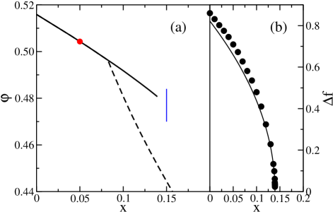
Figure 1: (a) dynamic phase diagram of a partially pinned hard sphere system. $x$ and $\varphi$ denote, respectively, the fraction of particles that are pinned and the volume fraction of all (mobile and pinned) particles. Solid line: discontinuous mode-coupling transition. Dashed line: localization transition (i.e. vanishing self-diffusion coefficient) sd . The filled circle and the thin vertical line indicate states for which the time dependence of the intermediate scattering function is shown in Fig. 2. (b) Circles: $x$ dependence of the discontinuity of the long-time limit of the normalized intermediate scattering function, $f(q)=F(q)/F(q;t=0)$, along the mode-coupling transition line shown in (a); thin solid line shows the square root singularity, $\Delta f\propto(x-x_{c})^{1/2}$.

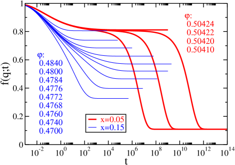
Figure 2: Time dependence of the normalized intermediate scattering function, $f(q;t)=F(q;t)/F(q;t=0)$. Thick solid lines: $x=0.05$ and $\varphi$ near the mode-coupling transition, solid circle in the left panel of Fig. 1. Thin solid lines: $x=0.15$ and $\varphi$ along the thin vertical line in Fig. 1a.

We used the numerical solution of Eqs. (1-5) to calculate the so-called collective and single-particle overlap functions. To define these functions we followed Berthier and Kob BKPRE2012 . Specifically, $Q(t)$ is proportional to the the probability that a spherical cell of radius $a$ is occupied at both $t=0$ and $t\to\infty$,

$$Q(t)\!\!\! = \!\!\!\frac{3}{4\pi a^{3}}\int d\mathbf{r}_{1}\int d\mathbf{r}_{2}F(|\mathbf{r}_{1}-\mathbf{r}_{2}|;t)\theta(a-r_{1})\theta(a-r_{2})$$ (7)

$$+Q_{\text{rand}}$$

where $F(r;t)$ is the inverse Fourier transform of $F(q;t)$ and $Q_{\text{rand}}=4\pi na^{3}/3$. In the definition of the single-particle overlap $Q_{\text{self}}(t)$, $F(r;t)$ is replaced by the inverse Fourier transform of of the self-intermediate scattering function $F^{s}(q;t)$ sd and $Q_{\text{rand}}$ is absent. To make connection with Ref. BKPRE2012 we chose $a=0.3$.

In Fig. 3 we show the time-dependence of the collective and single-particle overlaps for $\varphi=0.51$. For smaller $x$ our predictions are qualitatively similar to computer simulation results showed in Fig. 2(c) of Ref. BKPRE2012 . However, upon approaching the mode-coupling transition $Q(t)$ predicted by the theory shows a classic mode-coupling-like two step decay whereas the simulation results exhibit a continuous increase of both the intermediate-time plateau and the long-time plateau.

In Fig. 4a we show the length dependence of the so-called static overlap, i.e. the nontrivial part of the long time plateau of the collective overlap, $Q_{\infty}-Q_{\text{rand}}$, where $Q_{\infty}=\lim_{t\to\infty}Q(t)$. The length, $l=0.5x^{-1/3}$, is the so-called confining length BKPRE2012 . Perhaps fortuitously, for the range of lengths corresponding to non-glassy states, the values of $Q_{\infty}-Q_{\text{rand}}$ are quite close to those obtained from computer simulations. However, according to our mode-coupling approach an increase of $Q_{\infty}-Q_{\text{rand}}$ is followed by a discontinuity at the mode-coupling transition line whereas the values obtained from simulations increase continuously with decreasing $l$. Importantly, growing values of $Q_{\infty}-Q_{\text{rand}}$ are often associated with growing amorphous order and more specifically growing static point-to-set correlations. As indicated in Fig. 4a (and also noted in Ref. BKPRE2012 ), for the range of lengths corresponding to non-glassy states, $Q_{\infty}-Q_{\text{rand}}$ is dominated by the small $x$ contribution that originates from expression (6). This contribution has a rather trivial origin and it should not be associated with any many-body correlations CCT . It would be interesting to investigate whether there is a similar simple “baseline” contribution for other geometries considered in Ref. BKPRE2012 . Finally, in Fig. 4b we show the length dependence of the relaxation time $\tau$ defined through the single particle overlap, $Q_{\text{self}}(\tau)=e^{-1}$. We find that our mode-coupling approach overestimates the influence of the pinning on the relaxation time: the values of $\ln(\tau/\tau_{\infty})$, where $\tau_{\infty}$ is the relaxation time of the $l=\infty$ (i.e. un-pinned, $x=0$) system, are consistently above those obtained from computer simulations. We note that at large $l$, the length of the relaxation time seems to become consistent with the value of the dynamic correlation length obtained from the so-called inhomogeneous mode-coupling theory (IMCT) BBMRPRL2006 ; SFPRE2010 .

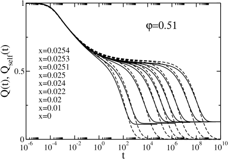
Figure 3: Time dependence of the collective overlap $Q(t)$ (solid lines) and the single particle overlap $Q_{\text{self}}(t)$ (dashed lines) for $\varphi=0.51$ and values of $x$ indicated in the figure.

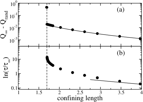
Figure 4: (a) Dependence of the overlap $Q_{\infty}$ on the confining length $l=0.5x^{-1/3}$ for $\varphi=0.51$. Solid line indicates the overlap originating from the small $x$ limit of $F(q)$, Eq. (6). (b) Dependence of the single-particle overlap relaxation time on the confining length $l=0.5x^{-1/3}$. Solid line shows the exponential dependence $\ln(\tau/\tau_{\infty})\propto\exp(-l/\xi_{\text{IMCT}})$ with $\xi_{\text{IMCT}}=1.66$ for $\varphi=0.51$ SFPRE2010 . Dashed vertical line through (a) and (b) indicates the mode-coupling transition.

In summary, we proposed an alternative mode-coupling approach for partially pinned systems. Our approach agrees qualitatively with the mean-field analysis of the $p$ spin model and with the results obtained from the RFOT theory. We showed that the contribution to the long-time limit of the collective overlap originating from the presence of pinning is dominated by the trivial small $x$ limit. This small $x$ contribution is not related to any growing point-to-set correlations.

We gratefully acknowledge the support of NSF Grant CHE 0909676. GS thanks G. Biroli and C. Cammarota for a discussion that inspired this work. We thank G. Biroli, L. Berthier, C. Cammarota and V. Krakoviack for comments on the manuscript.

References

- (1) K. Kim, Europhys. Lett. 61, 790 (2003).
- (2) K. Kim, K. Miyazaki and S. Saito, J. Phys.: Condens. Matter, 23 (2011) 234123.
- (3) C. Cammarota and G. Biroli, arXiv:1106.5513v2 (accepted for publication in PNAS).
- (4) V. Krakoviack, Phys. Rev. E 84, 050501(R) (2011).
- (5) L. Berthier and W. Kob, Phys. Rev. 85, 011102 (2012).
- (6) S. Karmakar, E. Lerner, and I. Procaccia, Physica A 391, 1001 (2012).
- (7) B. Charbonneau, P. Charbonneau and G. Tarjus, Phys. Rev. Lett. 108, 035701 (2012).
- (8) C. Cammarota and G. Biroli, Europhys. Lett. 98, 16011 (2012).
- (9) W.G. Madden and E. Glandt, J. Stat. Phys. 51, 537 (1988).
- (10) For a recent review and a comparison of quenched-annealed and partially pinned systems see V. Krakoviack, Phys. Rev. E 82, 061501 (2010).
- (11) See also a recent simulational study, J. Kurzidim, D. Coslovich, and G. Kahl, Phys. Rev. E 82, 041505 (2010).
- (12) J.-P. Bouchaud and G. Biroli, J. Chem. Phys. 121, 7347 (2004).
- (13) G. Biroli, J.-P. Bouchaud, A. Cavagna and P. Verrocchio, Nature Physics 4, 771 (2008).
- (14) A. Montanari and G. Semerjian, J. Stat. Phys. 125, 22 (2006).
- (15) W. Kob, S. Roldan-Vargas and L. Berthier, Nature Physics 8, 164 (2012).
- (16) P. Scheidler, W. Kob, and K. Binder, J. Phys. Chem. B 108, 6673 (2004).
- (17) W. Götze, Complex dynamics of glass-forming liquids: A mode-coupling theory (Oxford University Press, Oxford, 2008).
- (18) T. R. Kirkpatrick, D. Thirumalai, and P. G. Wolynes, Phys. Rev. A 40, 1045 (1989); V. Lubchenko and P. G. Wolynes, Annu. Rev. Phys. Chem. 58, 235 (2007).
- (19) B. Schmid and R. Schilling, Phys. Rev. E 81, 041502 (2010).
- (20) A. Ikeda and K. Miyazaki, Phys. Rev. Lett. 104, 255704 (2010).
- (21) P. Charbonneau, A. Ikeda, G. Parisi, and F. Zamponi, Phys. Rev. Lett. 107, 185702 (2011).
- (22) The derivation of the theory used in Ref. KrakPRE2011 was presented in V. Krakoviack, Phys. Rev. E 75, 031503 (2007); for an earlier, shorter account see also V. Krakoviack, Phys. Rev. Lett. 94, 065703 (2005).
- (23) For a derivation of mode-coupling equations for a Brownian systems see G. Szamel and H. Löwen, Phys. Rev. A 44, 8215 (1991).
- (24) While following the procedure of Refs. Goetze ; SL it is important to remember that the fluid density has non-vanishing correlations with the matrix density.
- (25) The details of the derivation will be presented elsewhere.
- (26) It should be emphasized that in the derivation of Eq. (1) we used an important simplification concerning static correlation functions of a partially pinned system KrakPRE2010 ; der .
- (27) G. Szamel, Europhys. Lett. 91, 56004 (2010).
- (28) E. Flenner and G. Szamel, Phys. Rev. E 72, 031508 (2005).
- (29) The theory for the self-intermediate scattering function will be presented elsewhere. This theory reproduces re-entrance in the tagged particle dynamics that was first predicted by Krakoviack [V. Krakoviack, Phys. Rev. E 79, 061501 (2009)].
- (30) A similar conclusion was reached in Ref. CCTPRL .
- (31) G. Biroli, J.-P. Bouchaud, K. Miyazaki, and D.R. Reichman, Phys. Rev. Lett. 97, 195701 (2006).
- (32) G. Szamel and E. Flenner, Phys. Rev. E 81, 031507 (2010).