Variance of the Galactic nuclei cosmic ray flux

Abstract

Context. Measurements of cosmic ray fluxes by the PAMELA and CREAM experiments show unexpected spectral features between 200 GeV and 100 TeV. They could be due to the presence of nearby and young cosmic ray sources. This can be studied in the myriad model, in which cosmic rays diffuse from point-like instantaneous sources located randomly throughout the Galaxy.

Aims. To test this hypothesis, one must compute the flux due to a catalog of local sources, but also the error bars associated to this quantity. This turns out not to be as straightforward as it seems, as the standard deviation is infinite when computed for the most general statistical ensemble. The goals of this paper are to provide a method to associate error bars to the flux measurements which has a clear statistical meaning, and to explore the relation between the myriad model and the more usual source model based on a continuous distribution.

Methods. To this end, we show that the quantiles of the flux distribution are well-defined, even though the standard deviation is infinite. They can be used to compute 68 % confidence levels, for instance. We also use the fact that local sources have known positions and ages to reduce the statistical ensemble from which random sources are drawn in the myriad model.

Results. We present a method to evaluate meaningful error bars for the flux obtained in the myriad model. In this context, we also discuss the status of the spectral features observed in the proton flux by CREAM and PAMELA.

1 Introduction

In the 1 GeV to 100 TeV energy range, cosmic ray (CR) nuclei that reach the Earth have a Galactic origin. They were accelerated in sources, the nature of which is still a subject of discussion and research, supernova driven shock waves being a good candidate. They subsequently reach the Earth, after diffusing in the Galactic magnetic field. The exact locations and ages of the supernova explosions are not known, and properties of Galactic cosmic rays are often studied under the assumption that sources form a distribution which is continuous, in space as in time. In the standard model of CR propagation, sources are modelled as a jelly which extends inside the Galactic disk and steadily injects particles in the interstellar medium (ISM). This picture has proven to be quite successfull so far. The CR spectra are actually dominated by sources which are distant from Earth (for instance see Fig. 8 in (Taillet et al. 2004)) and the continuous hypothesis is expected to be valid. On the other hand, this approach may fail, when one considers the high-energy end of the CR spectra, mainly produced by young sources. The flux at high energy could well be dominated by a handful of individual sources, the positions and ages of which have a strong influence on the spectrum. This is of tremendous importance as the latest measurements, such as those of CREAM (Yoon et al. 2011) or PAMELA (Adriani et al. 2011), exhibit spectral features which are difficult to understand in a continuous and steady-state modelling of CR sources.

In this article, we study the relation between the mean-field approach and the so-called “myriad model” ((Higdon et al. 2003)) where CR primary species, such as protons or helium nuclei, diffuse from point-like sources distributed randomly in space and time. In the myriad model, the flux of cosmic rays is a random variable. When averaged over many realisations of the possible positions and ages of the sources, the myriad model gives the same results as the continuous model, as expected.

However, we expect fluctuations from the average flux, from one realization to the other. If these fluctuations are small, then the myriad model predictions of the flux are robust and similar to that of the continuous model. In that case, the spectral features seen by CREAM and PAMELA should be explained within the continuous model. Invoking a distorted spectral injection spectrum at the sources (see for instance Yuan et al. (2011)) or a non-standard behaviour of the Galactic diffusion coefficient with energy are two possible, although unlikely, solutions. On the other hand, if the statistical fluctuations of the myriad model are large, it could be easier, and to some extent more natural, to explain the CREAM and PAMELA anomalies in terms of the particular history and morphology of the population of sources within which we live. If so, there is little reason to trust anymore the continuous model, on which most of CR studies are nevertheless based. The “real” sources could generate CR fluxes at the Earth quite different from those predicted in the conventional approach. Unfortunately, we do not know where and when the “real” supernova explosions took place. We are reduced to rely on statistics in order to gauge how probable are CR fluxes far from the values predicted by the continuous model.

The amplitudes of the statistical fluctuations of the myriad model have actually been recently studied through the standard deviation of the random variable associated to the CR proton flux (see e.g. (Blasi & Amato 2011)). This quantity turns out te be infinite, when computed without precautions. This unexpected result is, a priori, a severe blow against the mean-field approach on which most of the public codes of CR Galactic transport, such as galprop, dragon or usine, are based. These codes would have to be entirely modified. Abandoning the conventional CR model would have also drastic consequences on the problem of the astronomical dark matter (DM). The nature of this component, which contributes substantially to the mass budget of the universe, is still an unresolved issue. Weakly interacting massive particles (WIMP) have been invoked as a plausible solution. These putative DM species are expected to annihilate inside the Galactic DM halo, producing in particular rare antimatter cosmic rays such as positrons and antiprotons. Distortions in the spectra of these particles would be an indirect probe of the presence of WIMPs inside the Milky Way. Theoretical predictions have been based so far on the continuous CR model. They need to be entirely revisited should the myriad model replace the conventional scheme.

This article is devoted to the myriad model and to the issue arising from the infinite variance of the primary CR flux. We suggest two ways to solve this problem. First, we show that the statistical distribution of the flux is such that the confidence intervals are finite and well-defined, even though the variance is infinite. We study how the width of these intervals depends on the CR propagation model. Second, we notice that the divergence of the variance is due to the sources that are very close to the Earth and very young. In our Galaxy, theses objects are known actually, and the region in which we have catalogs of the sources should be excluded from the statistical ensemble of the myriad model, and rather treated as known sources. This paper explores the consequences of this approach.

2 Propagator for diffusive propagation from discrete sources

After their acceleration by supernova driven shock waves, primary cosmic ray (CR) nuclei subsequently propagate through the Galactic magnetic fields and bounce off their irregularities – the Alfvén waves. The resulting particle transport is well described by space diffusion with a coefficient

$$D(E)=D_{0}\;\beta\;\mathscr{R}^{\delta}\;\;,$$ (1)

which increases as a power law with the rigidity ${\mathscr{R}}\equiv{p}/{Z}$ of the particle. In addition, since these scattering centers move with a velocity $V_{a}\sim$ 20 to 100 km s^-1, a second order Fermi mechanism is responsible for some diffusive re-acceleration which turns out to be mostly relevant at low energy, below a few GeV. Since we are interested here in the excess in CR protons and helium nuclei measured by CREAM, and more recently by PAMELA, we will disregard diffusive re-acceleration as well as energy losses which are also negligible at high energy. In addition to space diffusion, Galactic convection wipes cosmic rays away from the Galactic disk with a velocity $V_{C}\sim$ 5 to 15 km s^-1. The master equation for the space and energy number density $\psi\equiv{dn_{p}}/{dT_{p}}$ of, say, CR protons with kinetic energy $T_{p}$ takes into account space diffusion and Galactic convection

$${\displaystyle\frac{\partial\psi}{\partial t}}\,+\,\partial_{z}\!\left(V_{C}\,\psi\right)\,-\,D\,\triangle\psi\,=\,q_{\rm eff}=q_{\rm acc}\,-\,q_{\rm col}\;\;.$$ (2)

This equation applies to any nuclear species – protons and helium nuclei in particular – as long as the effective rate of production $q_{\rm eff}$ is properly accounted for. This general framework, summarized in Eq. (2), is generally implemented within an axisymmetric two-zone model which is extensively discussed in Maurin et al. (2001) or Donato et al. (2001), and whose salient features are briefly recalled here.

The CR diffusive halo (DH) is pictured as a thick wheel which matches the circular structure of the Milky Way. The Galactic disk of stars and gas – where primary CR protons and helium nuclei are accelerated – lies in the middle. It extends radially 20 kpc from the center and has a half-thickness $h$ of 100 pc. Confinement layers, where cosmic rays are trapped by diffusion, lie above and beneath that disk. The interGalactic medium starts at the vertical boundaries $z=\pm L$ as well as beyond a radius of $r=R_{\rm gal}=$ 20 kpc. Notice that the half-thickness $L$ of the DH is not known and possible values range from 1 to 15 kpc. The diffusion coefficient $D$ is taken to be the same everywhere while the convective velocity is exclusively vertical, with component

$$V_{C}(z)=V_{C}\,{\rm sign}(z)\;\;.$$ (3)

The Galactic wind – produced by the bulk of the disk stars like the Sun – drifts away from them along the vertical directions, hence the particular form assumed here for $V_{C}$. The effective production term $q_{\rm eff}$ takes into account the release of primary CR nuclei described by the positive term $q_{\rm acc}$ as well as a negative contribution that accounts for their interactions with the interstellar gas of the disk with rate $q_{\rm col}$. In most propagation codes, the injection of cosmic rays is described by a smooth function of space and is constant in time. In this article, we treat supernova explosions as point-like events. The production rate of CR nuclei through acceleration is given by

$$q_{\rm acc}(\mathbf{x}_{S},t_{S})={\displaystyle\sum_{n\in\mathscr{P}}}\,\,q_{n}\,\,\delta^{3}(\mathbf{x}_{S}-\mathbf{x}_{n})\,\delta(t_{S}-t_{n})\;\;,$$ (4)

where each source $i$ belonging to the population $\mathscr{P}$ of supernovae contributes a factor $q_{i}$ at position $\mathbf{x}_{i}$ and time $t_{i}$. The collisions of CR nuclei on the hydrogen and helium atoms of the interstellar medium (ISM) tend to deplete the high energy regions of their spectra. In the case of CR protons, which we will use throughout this section as an illustration, they act as a negative source term for the energy bin located at $T_{p}$, with amplitude

$$q_{\rm col}(\mathbf{x}_{S},t_{S})=2\,h\,\delta(z_{S})\;\Gamma_{p}\;\psi(\mathbf{x}_{S},t_{S})\;\;.$$ (5)

The ISM is distributed within an infinitely thin disk, hence the presence of a $\delta(z_{S})$ function in the previous expression. The collision rate may be expressed as

$$\Gamma_{p}=v_{p}\;\left(\sigma_{p{\rm H}}\,n_{\rm H}\;+\;\sigma_{p{\rm He}}\,n_{\rm He}\right)\;\;,$$ (6)

where the densities $n_{\rm H}$ and $n_{\rm He}$ have been respectively averaged to $0.9$ and $0.1$ cm^-3. The total proton-proton cross section $\sigma_{p{\rm H}}$ has been parameterized according to Nakamura et al. (2010) while $\sigma_{p{\rm He}}$ is related to $\sigma_{p{\rm H}}$ by the Norbury & Townsend (2007) scaling factor $4^{2.2/3}$. Similar scaling factors have been used in order to derive the CR helium nuclei collision cross sections from the proton case.

2.1 Solution of the diffusion equation

Our description of the propagation of CR protons through the DH, and of any other CR nucleus for that matter, relies on the existence of the propagator $\mathscr{G}_{\!p}$. This Green function translates the probability for a CR proton injected at position $\mathbf{x}_{S}\equiv(x_{S},y_{S},z_{S})$ and time $t_{S}$ to travel through the Galactic magnetic field until it reaches, at time $t$, an observer located at $\mathbf{x}\equiv(x,y,z)$. The CR proton density at the Earth may be expressed as the convolution over space and time of the Green function $\mathscr{G}_{\!p}$ with $q_{\rm acc}$

$$\psi(\mathbf{x},t)={\displaystyle\int_{-\infty}^{\,t}}dt_{S}\,{\displaystyle\int_{\rm DH}}d^{3}\mathbf{x}_{S}\;\mathscr{G}_{\!p}\left(\mathbf{x},t\,\leftarrow\,\mathbf{x}_{S},t_{S}\right)\;q_{\rm acc}(\mathbf{x}_{S},t_{S})\;\;,$$ (7)

where $q_{\rm acc}(\mathbf{x}_{S},t_{S})$ is the CR proton injection rate at the source located at $\mathbf{x}_{S}$ and at time $t_{S}$. Notice that for a population $\mathscr{P}$ of point-like sources, the injection rate $q_{\rm acc}$ is given by Eq. (4) which, once plugged in the previous expression for $\psi$, leads to the proton flux at the Earth

$$\Phi={\displaystyle\frac{v_{p}}{4\pi}}\times\left\{\psi\equiv{\displaystyle\sum_{n\in\mathscr{P}}}\;\mathscr{G}_{\!p}\left(\mathbf{x}_{\odot},t=0\,\leftarrow\,\mathbf{x}_{n},t=t_{n}\right)\times q_{n}\right\}\;\;.$$ (8)

The Green function $\mathscr{G}_{\!p}$ plays a crucial role in our analysis and is the ideal tool to study the effect of the discreteness of the sources. It is a solution of the CR transport equation

$${\displaystyle\frac{\partial\,\mathscr{G}_{\!p}}{\partial\,t}}\,+\,\partial_{z}\left(V_{C}\,\mathscr{G}_{\!p}\right)\,-\,D\,\triangle\,\mathscr{G}_{\!p}\,+\,2\,h\,\delta(z)\,\Gamma_{p}\,\mathscr{G}_{\!p}=\delta^{3}(\mathbf{x}-\mathbf{x}_{S})\,\delta(t-t_{S})\;\;.$$ (9)

The resolution of this equation is presented in Appendix A.

2.2 Diffusion parameters

The computed flux depends on the diffusion parameters. The results will be presented for three benchmark sets of diffusion parameters, consistent with the energy dependance of the B/C ratio (Maurin et al. 2001). They are labelled “min”, “med” and “max”, according to the value of $L$. The values are indicated in Table 1.

Table 1: Diffusion parameters for the three benchmark models

model	$D_{0}\;(\text{kpc}\cdot\text{My}^{-1})$	$\delta$	$L\;(\text{kpc})$	$V_{c}\;(\text{km}\cdot\text{s}^{-1})$
min	0.0016	0.85	1	13.5
med	0.0112	0.7	4	12
max	0.0765	0.46	15	5

3 Mean flux

The flux at Solar position is obtained by summing the contributions of all the point sources. The mean value can be computed, once the distribution of sources is known. We first provide the result for a homogeneous distribution of sources, as an analytic expression can be found in this case. We then turn to a more realistic distribution.

3.1 Homogeneous distribution of sources

The average flux from one point source, drawn from a statistical ensemble with distances ranging from $R_{\text{min}}$ to $R_{\text{max}}$ and ages from $t_{\text{min}}$ to $t_{\text{max}}$, is given by averaging $\mathscr{G}_{1}\equiv\mathscr{G}_{p}$ over distances and times. To get an order of magnitude estimate, we first consider that the sources are distributed evenly in space and time in the Galactic disk, which is assumed to be infinitely thin and to extend to $R_{\text{max}}\to\infty$. We obtain

$$\langle\mathscr{G}_{1}\rangle=\frac{1}{\pi R_{\text{max}}^{2}t_{\text{max}}}\int_{0}^{R_{\text{max}}}2\pi r\,dr\int_{t_{\text{min}}}^{t_{\text{max}}}\frac{d\tau}{4\pi DL\tau}e^{-r^{2}/4D\tau}\sum_{n}e^{-k_{n}^{2}D\tau}$$

Considering $\nu$ sources per unit time and unit area in the disk, the average flux from $N=\nu\pi R_{\text{max}}^{2}t_{\text{max}}$ sources is given by

$$\langle\mathscr{G}_{N}\rangle=N\langle\mathscr{G}_{1}\rangle=\frac{\nu}{4\pi DL}\int_{0}^{R_{\text{max}}}2\pi r\,dr\int_{0}^{t_{\text{max}}}\frac{d\tau}{\tau}e^{-r^{2}/4D\tau}\sum_{n}e^{-k_{n}^{2}D\tau}$$

By integrating over time ($t_{\text{max}}\to\infty$) and using (Gradshteyn et al. (2007) 3.471.9)

$${\displaystyle\int_{0}^{\infty}}\,x^{\nu-1}\,e^{-\beta/x-\gamma x}\;dx=2\left(\frac{\beta}{\gamma}\right)^{\nu/2}K_{\nu}\left(2\sqrt{\beta\gamma}\right)\;\;,$$ (10)

where $K_{\nu}$ is the $\nu$-th order modified Bessel function of the second kind, leads to

$$\langle\mathscr{G}_{N}\rangle=\nu\int_{0}^{R_{\text{max}}}2\pi r\mathscr{G}_{\text{steady}}(r)\,dr$$

where $\mathscr{G}_{\text{steady}}$ stands for the one source steady-state propagator, given by

$$\mathscr{G}_{\text{steady}}\left(\mathbf{x}\,\leftarrow\,\mathbf{x}_{S}\right)=\frac{1}{2\pi DL}\sum_{n=1}^{\infty}K_{0}\left(\rho\sqrt{\alpha_{n}/D}\right).$$ (11)

Finally, using $\int x\,K_{0}(x)\,dx=-x\,K_{1}(x)$, we have

$$\begin{split}\langle\mathscr{G}_{N}\rangle=\frac{\nu}{D}\sum_{n=0}^{\infty}\frac{2}{(2n+1)\pi}&\left\{R_{\text{min}}K_{1}\left(\frac{2n+1}{2}\frac{\pi R_{\text{min}}}{L}\right)\right.\\ &\left.-R_{\text{max}}K_{1}\left(\frac{2n+1}{2}\frac{\pi R_{\text{max}}}{L}\right)\right\}\end{split}$$ (12)

For an infinite disk, $R_{\text{min}}=0$ and $R_{\text{max}}\to\infty$, so that, using $xK_{1}(x)\to 1$ when $x\to 0$,

$$\langle\mathscr{G}_{N}\rangle=\frac{\nu L}{D}\sum_{n=0}^{\infty}\left(\frac{2}{(2n+1)\pi}\right)^{2}$$

It can be shown that $\sum_{n}1/(n+1/2)^{2}=\pi^{2}/2$, and finally for the infinite disk,

$$\langle\mathscr{G}_{N}\rangle=\frac{\nu L}{2D}$$

which is what is also obtained by directly solving the diffusion equation in steady state. The mean value of the flux from randomly distributed point sources is equal to the steady-state flux obtained with a continuous source distribution. This is also true in more general cases, thick disk, finite radius, with wind and spallation.

3.2 Realistic distribution of sources

We now consider the case of a general distribution of sources, with a radial distribution in the Galactic disk, as well as a distribution across the thickness of the disk. It is quite well accepted that up to energies corresponding to the knee, cosmic rays accelerators are supernova remnants (SNR). Unfortunately, supernovae are pretty rare events and their spatial distribution is difficult to measure accurately. However, as pulsars are created in SNR and are easier to detect, it is a fair asumption that the cosmic ray sources follow the pulsar distribution. In this work we suppose that the radial profile of sources follows the pulsar distribution given in Yusifov & Küçük (2004),

$$f_{r}(r_{s})=\left(\frac{r_{s}+0.55}{8.5+0.55}\right)^{1.64}\exp\left\{-4.01\left(\frac{r_{s}-8.5}{8.5+0.55}\right)\right\}$$

where distances are expressed in kpc. The distribution along the $z$ axis is given by

$$f_{s}(z_{s})=\exp{\left(-\frac{|z_{s}|}{z_{0}}\right)}$$

where $z_{0}$ is set to the half-thickness of the Galactic disk, $z_{0}=h$. In this section, $z_{s}$, $r_{s}$, $\theta_{s}$ and $t_{s}$ refer to the position and age of sources. The solar system is located at $r_{\odot}=8.5\;\text{kpc}$, $\theta=0$ and $z=0$. Moreover we define $\rho(r_{s},\theta_{s})$ as the distance from a source to the Solar System:

$$\rho(r_{s},\theta_{s})=\sqrt{(r_{\odot}-r_{s}\cos\theta_{s})^{2}+r_{s}^{2}\sin^{2}\theta_{s}}$$

We evaluate the scatter of the flux that arises when we consider point-like sources with positions and ages following a given probability distribution. The sources are supposed to be independent, so the mean value of the propagator coming from all the $N$ sources is just given by :

$$\begin{split}\langle\mathscr{G}_{N}\rangle=&N\times\langle\mathscr{G}_{1}\rangle=NA\int 2\pi\,r_{s}dr_{s}\int d\theta_{s}\int dz_{s}\int dt_{s}\\ &f_{\theta}(\theta)\,f_{r}(r_{s})\,f_{z}(z_{s})\,f_{t}(t_{s})\mathscr{G}_{N}\left(r_{s},\theta_{s},t_{s}\right)\end{split}$$ (13)

Assuming cylindrical symmetry and a uniform age distribution, up to a maximum age $T_{\text{max}}$, the normalization factor $A$ is given by,

$$\frac{1}{A}=2\pi\,T_{\text{max}}\int_{Galaxy}rf_{r}(r)\,f_{z}(z)drdz$$

We find (the antisymmetric part of the propagator vanishes at $z=0$)

$$\begin{split}\langle\mathscr{G}_{N}\rangle&=N\int r_{s}dr_{s}dz_{s}dt_{s}d\theta_{s}Af_{r}(r_{s})\exp\left(-\frac{|z_{s}|}{z_{0}}\right)\\ &\times\frac{1}{4\pi Dt_{s}}\exp\left(\frac{-V_{c}|z_{s}|}{2D}\right)\exp(-\frac{\rho^{2}(r_{s},\theta_{s})}{4Dt_{s}})\\ &\times\sum_{n=1}^{\infty}\frac{\exp\left(-(\alpha_{n})t_{s}\right)}{C_{n}}\sin(k_{n}L)\sin(k_{n}(L-|z_{s}|))\end{split}$$

We separate the integration and define

$$\langle J_{z}\rangle_{n}=\frac{\sin(k_{n}L)}{C_{n}}\int_{-L}^{L}\exp\left(-\frac{|z_{s}|}{z_{0}}\right)\exp\left(-\frac{V_{c}|z_{s}|}{2D}\right)\sin(k_{n}(L-|z_{s}|))$$ (14)

The integration is easy using the exponential form of sinus and leads to

$$\begin{split}\langle J_{z}\rangle_{n}&=\frac{\sin(k_{n}L)}{C_{n}}\frac{2}{(V_{c}/2D+1/h)^{2}+k_{n}^{2}}\\ &\times\left(\left(\frac{V_{c}}{2D}+\frac{1}{h}\right)\sin(k_{n}L)-kn\left(\cos(k_{n}L)-e^{-L\left(\frac{V_{c}}{2D}+\frac{1}{h}\right)}\right)\right)\end{split}$$ (15)

The integration over time ($t_{\text{max}}\to\infty$) is made using Eq. 10 :

$$\begin{split}\int_{0}^{\infty}\frac{1}{4\pi Dt_{s}}&\exp\left(-\frac{\rho^{2}(r_{s},\theta_{s})}{4Dt_{s}}\right)\exp(-\alpha_{n}t_{s})dt_{s}\\ &=\frac{1}{2D\pi}K_{0}\left(\rho(r_{s},\theta_{s})\sqrt{\frac{\alpha_{n}}{D}}\right)\end{split}$$ (16)

Then we can write the mean value as :

$$\langle\mathscr{G}_{N}\rangle=N\frac{A}{2D\pi}\int dr_{s}d\theta_{s}r_{s}f_{r}(r_{s})f_{\theta}(\theta_{s})\sum_{n}K_{0}\left(\rho(r_{s},t_{s})\sqrt{\frac{\alpha_{n}}{D}}\right)\langle J_{z}\rangle_{n}$$ (17)

This result is integrated numerically over the two coordinates $r_{s}$ and $\theta_{s}$. The mean flux is then given by

$$\langle\Phi\rangle=\langle\mathscr{G}_{N}\rangle\frac{\rm v}{4\pi}g(E)$$

Where $g(E)$ is the source energy injection term. We checked that this calculation gives the same result as the steady state model. In the next section, we perfom the calculation of the variance associated to the flux.

4 Statistical analysis : variance of the flux

The flux obtained in the myriad model depends on the exact positions and ages of all the sources. It is bound to be different from the mean values computed above, at some level. How different from the mean value are likely to be the typical fluxes in the myriad model? In order to address this question, the usual method is to compute the standard deviation associated to the flux, considered as a random variable.

4.1 Realistic distribution of sources

The variance of the propagator for one source is defined as

$$\sigma_{1}^{2}=\langle\mathscr{G}_{1}^{2}\rangle-\langle\mathscr{G}_{1}\rangle^{2}$$

The variance for $N$ independent sources is given by

$$\sigma_{N}^{2}=N\sigma_{1}^{2}$$

We must compute the average value of $\mathscr{G}_{1}^{2}$, given by

$$\begin{split}\langle\mathscr{G}_{1}^{2}\rangle&=\int dr_{s}dz_{s}dt_{s}d\theta_{s}Ar_{s}f_{r}(r_{s})\exp\left(-\frac{|z_{s}|}{z_{0}}\right)\\ &\times\left(\frac{1}{4\pi Dt_{s}}\right)^{2}\exp\left(-\frac{V_{c}|z_{s}|}{D}\right)\exp\left(-\frac{\rho^{2}(r_{s},\theta_{s})}{2Dt_{s}}\right)\\ &\times\sum_{n=1}^{\infty}\sum_{m=1}^{\infty}\frac{\exp\left(-(\alpha_{n}+\alpha_{m})t_{s}\right)}{C_{n}C_{m}}\\ &\sin(k_{n}L)\sin(k_{m}L)\sin(k_{n}(L-|z_{s}|))\sin(k_{m}(L-|z_{s}|))\end{split}$$ (18)

At fixed $m$ and $n$, we define

$$\begin{split}\langle\mathscr{G}_{z}^{2}\rangle_{n,m}\equiv\frac{\sin(k_{n}L)\sin(k_{m}L)}{C_{n}C_{m}}\int_{-L}^{L}&dz_{s}\exp\left(-|z_{s}|\left(\frac{V_{c}}{D}+\frac{1}{h}\right)\right)\\ &\sin(k_{n}(L-|z_{s}|))\sin(k_{m}(L-|z_{s}|))\end{split}$$ (19)

This is easily computed, and we can integrate the time distribution to get the variance from sources of all ages :

$$\begin{split}\langle\mathscr{G}_{1}^{2}\rangle=A\sum_{n,m}\langle\mathscr{G}_{z}^{2}\rangle_{n,m}\int&dt_{s}dr_{s}d\theta_{s}r_{s}f_{r}(r_{s})\exp(-(\alpha_{n}+\alpha_{m})t_{s})\\ &\times\frac{1}{16\pi^{2}D^{2}t_{s}^{2}}\exp\left(-\frac{2\rho^{2}(r_{s},\theta_{s})}{4Dt_{s}}\right)\end{split}$$ (20)

Using Eq. 10 and considering $t_{\text{max}}\to\infty$

$$\begin{split}\int_{0}^{\infty}&dt_{s}\left(\frac{1}{4\pi Dt_{s}}\right)^{2}\exp\left(-\frac{\rho^{2}}{2Dt_{s}}\right)\exp(-(\alpha_{n}+\alpha_{m})t_{s})\\ &=\sqrt{2(\alpha_{n}+\alpha_{m})D}\frac{1}{8\pi^{2}D^{2}}\frac{1}{\rho}K_{1}\left(\rho\sqrt{\frac{2(\alpha_{n}+\alpha_{m})}{D}}\right)\end{split}$$ (21)

we find

$$\begin{split}\langle\mathscr{G}_{1}^{2}\rangle=&A\sum_{n,m}\langle\mathscr{G}_{z}^{2}\rangle_{n,m}\frac{1}{8\pi^{2}D^{2}}\sqrt{2\left(\alpha_{m}+\alpha_{n}\right)D}\int_{0}^{R_{\text{max}}}r_{s}dr_{s}\\ &\times\int_{0}^{2\pi}d\theta_{s}\frac{1}{\rho(r_{s},\theta_{s})}K_{1}\left(\rho(r_{s},\theta_{s})\sqrt{2\frac{\alpha_{m}+\alpha_{n}}{D}}\right)f_{r}(r_{s})\end{split}$$ (22)

We are interested in the behaviour of this quantity at the lower bound in $r$. When $r\sqrt{2(\alpha_{m}+\alpha_{n})/D}\ll 1$, the property $K_{1}(x)\to 1/x$ as $x\to 0$ can be used to show that the above integral diverges as $\ln(R_{\text{min}})$ as the lower bound $R_{\text{min}}$ of the spatial integral goes to zero. The spatial distribution probability is $f_{r}\sim 1$ when $r\to 0$, so that

$$\langle\mathscr{G}_{1}^{2}\rangle\sim\frac{A}{4\pi D}\ \sum_{n,m}\langle\mathscr{G}_{z}^{2}\rangle_{n,m}\ln R_{\text{min}}$$ (23)

4.2 Divergence of the variance: how bad is it?

The mean value, computed considering $r_{s}$ from $r_{s}=0$ to $r_{s}=20$ kpc and $t_{s}$ from $t_{s}=0$ to $t_{s}=\infty$ is equal to the flux obtained in the steady-state model, as commonly obtained in propagation theories. But as we have just seen, the calculation related to the standard deviation of this quantity diverges, when we allow the possibility of sources that are close ($r_{s}\to 0$) and young ($t_{s}\to 0$), as already noticed before ((Blasi & Amato 2011)).

The standard deviation is usually interpreted as the typical spread of the random values around the mean, and a large standard deviation could be interpreted as if the actual value of the flux had a disturbingly large probability to be very far from the mean value.

One could argue that the problem we considered is physically irrelevant, as we know for sure that there is no supernova remnant with zero age and null distance to the Earth. One can impose a lower cut-off in ages and distances, based on observations. However, even with reasonable values for the cut-off, the variance can be finite but large (see section 4.3). One can also adjust the cut-off in order to eliminate the very rare events that make the standard deviation very large, without contributing significantly to the the mean value. This is the approach adopted by Blasi & Amato (2011). These authors use a cut-off given by $t_{\text{min}}=R_{\text{max}}/\sqrt{4\nu D(E)}$. This condition gives a fair order of magnitude of the spread of the values around the mean. It is difficult though to interpret it in rigourous statistical terms. Actually, the value of the variance depends quite strongly on the exact position of the cut-off, as featured in Fig. 1 where the evolution of the mean and the standard deviation of the total proton flux derived with the max model at 10 TeV is presented. Choosing $t_{\text{min}}/2$ or $2\times t_{\text{min}}$ rather than $t_{\text{min}}$, for instance, has a small effect on the mean but has a drastic effect on the standard deviation. The value chosen by Blasi & Amato (2011) is indicated by an arrow on the figure. The mean obtained with this cut-off is about 10 % smaller than the true mean. A lower cut-off would give a more precise mean value, but a much larger variance.

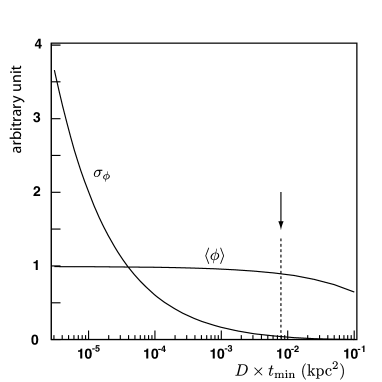
Figure 1: Evolution of the mean value and of the standard deviation of the flux with the age cut-off $t_{\text{min}}$. The cut-off obtained with the prescription $t_{\text{min}}=R_{\text{max}}/\sqrt{4\nu D(E)}$ (see text) is indicated with an arrow. This is for the max model, at an energy of 10 TeV.

This confusing situation, where some rare events have a very small contribution to the mean, but give rise to a very large standard deviation, is not uncommon in physics (Levy flights, Cauchy distribution). The total flux $\phi$ is the sum of a myriad of $N$ individual contributions $\varphi_{i}$ from single sources. Assuming that these contributions are not correlated with each other allows to relate simply the means and variances of the total and single source fluxes through

$$\langle\phi\rangle=N\times\langle\varphi\rangle\;\;\;{\rm and}\;\;\;\sigma_{\phi}^{2}=N\times\sigma_{\varphi}^{2}=N\langle\varphi^{2}\rangle\,-\,\frac{\langle\phi\rangle^{2}}{N}.$$ (24)

We show in the appendix that the probability $p(\varphi)$ of measuring a single source flux $\varphi$ is given by $p(\varphi)\propto\varphi^{-8/3}$ for objects located in a thick disk and $p(\varphi)\propto\varphi^{-7/3}$ for sources located in a thin disk, in the limit where $\varphi\to\infty$. The standard deviation $\sigma_{\phi}$ of the total flux is related to the integral $\langle\varphi^{2}\rangle=\int\varphi^{2}\,p(\varphi)\,d\varphi$, which diverges as $\varphi\to\infty$. For such a distribution with an infinite second moment, the central limit theorem does not hold, at least in its usual form. In this case, the standard deviation is not a good estimator of the typical spread of the values around the mean (in particular the probability distribution function $p(\phi)$ is no longer Gaussian), and there is no use trying to regularize this quantity by applying cut-offs. Notice that the average value $\langle\phi\rangle$ is still well-defined, as $\langle\varphi\rangle=\int\varphi\,p(\varphi)\,d\phi$ is convergent, and more to the point, the confidence intervals of the global probability distribution $p(\phi)$ are well-defined too, since the integral of $p(\varphi)$ is well-behaved. The spread of the random values of the total flux around its mean $\langle\phi\rangle$ can then be studied by computing the quantiles associated to the probability distribution $p(\phi)$, rather than using the standard deviation which has no clear statistical relevance in this case.

All this discussion arises from the fact that, in the myriad model, there is a non-vanishing probability to find sources which are arbitrarily close and young. Although the variance $\sigma_{\phi}$ cannot be defined in this case, we can still infer the global distribution function $p(\phi)$ and delineate intervals inside which the total fux $\phi$ is mostly expected. Another possibility is to take advantage of the solid information which has been collected on these young and nearby sources, whose statistical properties are disconcerting. We can actually remove a space-time region around the Earth containing the very close and very young sources of our Galaxy, and replace them by a catalog, built from observations.

In what follows, we investigate these points in further details. First we study how the standard deviation $\sigma_{\phi}$ can be regularized by applying some cut-offs related to astronomical information about the sources. We then focus on the confidence intervals of $p(\phi)$ and we show that they are well-defined, with no need of a particular cut-off. Finally, we take into account the astronomical knowledge about the local sources of cosmic rays and explore in greater detail how introducing such a catalog improves our statistical analysis.

4.3 Regularisation by cutting off the ages

From observations of the Solar neighbourhood, we have a good idea of the distribution of sources which are young and close. Given the age $t_{\text{min}}$ of the youngest local supernova remnant, one can compute the mean value and standard deviation of the total flux $\phi$, by applying that cut-off $t_{\text{min}}$ to the age distribution.

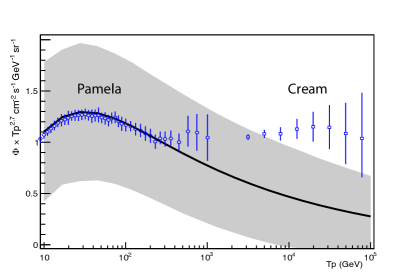
Figure 2: Proton flux obtained for the min diffusion model (see below) and a source frequency $\mu=3\;\text{century}^{-1}$. The band displays the standard deviation $\sigma_{\phi}$ obtained analytically, with a lower cut-off on the ages of the sources $t_{\text{min}}=100\;\text{years}$. The blue symbols indicate the flux measured by CREAM (Yoon et al. 2011) and PAMELA (Adriani et al. 2011).

For the sake of illustration, Fig. 2 features the mean value $\langle\phi\rangle$ and the standard deviation $\sigma_{\phi}$ of the total proton flux using a lower cut-off of $t_{\text{min}}=100\;\text{yr}$ in the source distribution, for the min set of propagation parameters. On the same figure we have also plotted the data points from the CREAM and PAMELA experiments. With the chosen value for the cut-off, the standard deviation at high energies remains of the same order of magnitude as the flux. The relative value of the standard deviation, ${\sigma_{\phi}}/{\langle\phi\rangle}$, is fairly independent of the energy. This trend can be shown analytically to hold for sources located in a thin disk. In the framework of a purely diffusive model (no wind/spallation), the relative dispersion can be actually approximated by

$$\frac{\sigma_{\phi}}{\langle\phi\rangle}\sim\frac{R}{4L\sqrt{2\nu t_{\text{min}}}}\;\;.$$ (25)

This ratio does not depend on the diffusion coefficient $D$, hence it does not depend on energy. It is of order or unity for $t_{\text{min}}\sim 100\;\text{yr}$.

For sources distributed in a disk having a finite thickness $h$, one gets the same result as before as long as $h\ll\sqrt{Dt_{\text{min}}}$. In the opposite limit, one finds

$$\frac{\sigma_{\phi}}{\langle\phi\rangle}\propto D^{1/4}\;\;.$$ (26)

In both cases, the relative standard deviation does not vary much with energy.

The value of $\sigma_{\phi}/\langle\phi\rangle$ depends sensitively on the chosen cut-off $t_{\text{min}}$. For a very low value of $t_{\text{min}}$, the standard deviation is very large. Conversely, for larger values of $t_{\text{min}}$, the standard deviation decreases, and the average value $\langle\phi\rangle$ starts to be affected by the cut-off, as shown in Fig. 1.

4.4 The variance is infinite but the confidence levels are finite

The variance of the flux being infinite does not necessarily imply that the random values are typically very different from the mean. To illustrate this affirmation, consider the case of a unique point-like steady-state source located in the Galactic disk, with cosmic ray diffusion taking place in a boundless space. The solution of the diffusion equation is given by $\varphi=a/r$ where $a$ is a constant. Assuming that this source is uniformly distributed inside a disk of radius $R$ leads to the probability distribution function

$$dp=\frac{2\pi r\,dr}{\pi R^{2}}=\frac{2r\,dr}{R^{2}}\;\;.$$ (27)

We can readily infer the mean flux

$$\langle\varphi\rangle=\int_{0}^{R}\,\frac{a}{r}\,\frac{2r\,dr}{R^{2}}=\frac{2a}{R}\;\;,$$ (28)

and the average value of the flux squared

$$\langle\varphi^{2}\rangle=\int_{\epsilon}^{R}\,\frac{a^{2}}{r^{2}}\,\frac{2r\,dr}{R^{2}}=\frac{a^{2}}{R^{2}}\ln\left(\frac{R}{\epsilon}\right)\;\;,$$ (29)

where we have introduced a cut-off value $\epsilon$ at the lower end of the radial distribution, to exhibit the divergence of $\langle\varphi^{2}\rangle$. The variance of $\varphi$ goes to infinity as $\epsilon\to 0$.

However, the distribution of $\varphi$ (which is what we are really interested in) is well-behaved. From the relation between $r$ and $\varphi$, we can write $dr={a\,d\varphi}/{\varphi^{2}}$ so that

$$dp(\varphi)=\frac{2r\,dr}{R^{2}}=\frac{2a^{2}\,d\varphi}{R^{2}\,\varphi^{3}}\;\;.$$ (30)

The probability that the flux is smaller than a given value $\Phi$ may be expressed as

$$P(<\Phi)=\int_{\varphi(r)}^{\varphi(R)}dp(\varphi)=1\,-\,\frac{a^{2}}{R^{2}\Phi^{2}}\;\;,$$ (31)

provided that $\Phi>\Phi_{0}\equiv a/R$. Introducing the Heavyside distribution $\Theta$ leads to

$$P(>\Phi)=\frac{a^{2}}{R^{2}\Phi^{2}}\,\Theta\left(\Phi-\frac{a}{R}\right)=\frac{\langle\varphi\rangle^{2}}{4\,\Phi^{2}}\,\Theta\left(\Phi-\frac{\langle\varphi\rangle}{2}\right)\;\;.$$ (32)

The probability that $\Phi>10\,\langle\varphi\rangle$ is only 1/400, even though the variance is infinite. Actually, the flux is more likely to be lower than the mean value, whereas one might have guessed the opposite, considering the divergence of the variance.

When $N$ sources are considered, the mean flux value and the variance are both just multiplied by $N$. The probability distribution $p_{N}(\phi)$ for the flux can be obtained by recurrence from

$$p_{N}(\phi)=\int p(\varphi)\,p_{N-1}(\phi-\varphi)\,d\varphi\;\;.$$ (33)

These are displayed in Fig. 4. The variance still diverges. In the high-$\phi$ region, the flux is dominated by the contribution of a single source and the probability distribution is given by

$$\frac{dp_{N}}{d\phi}=N\,\frac{dp}{d\varphi}=\frac{2Na^{2}}{R^{2}\phi^{3}}\;\;.$$ (34)

For $N=100$ sources, the probability that $\phi>2\,\langle\phi\rangle$ is $2.5\times 10^{-3}$ and $P(\phi>10\,\langle\phi\rangle)$ is vanishingly small.

Figure 3: Probability that the flux $\varphi=a/r$ is greater than $\phi$, for a unique point source drawn randomly in the disk, within a distance $R$.

Figure 4: Probability distribution of $\phi/N$ for $N=1$, 10 and 100 sources.

If we now consider time-dependent sources spread homogeneously inside an infinite DH with pure diffusion, the variance is given by the integral

$$\sigma_{\varphi}^{2}\propto\int dt\int 4\pi r^{2}\,dr\,\frac{1}{(4\pi Dt)^{3/2}}\,e^{-r^{2}/2Dt}\;\;,$$ (35)

which diverges with the lower cut-off in ages as ${1}/{\sqrt{t_{\text{min}}}}$. For a 3D homogeneous distribution of steady-state sources, $\sigma_{\varphi}$ does not diverge (see Table 2). For the sake of illustration, Fig. 5 presents histograms for the flux obtained with the propagator discussed in Sec. 2, at several energies.

Table 2: Divergence of the variance

	2D	3D
steady-state	$\langle\varphi\rangle$ finite $\langle\varphi^{2}\rangle\to\infty$	$\langle\varphi\rangle$ finite $\langle\varphi^{2}\rangle$ finite
time-dependent	$\langle\varphi\rangle$ finite $\langle\varphi^{2}\rangle\to\infty$	$\langle\varphi\rangle$ finite $\langle\varphi^{2}\rangle\to\infty$

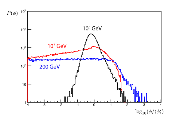
Figure 5: Examples of histograms of fluxes for the “min” cosmic ray propagation model.

4.5 Quantiles of the total flux

From now on, we show the quantiles associated to the fluxes. These are defined as regions with a given probability to find the flux. In Fig. 6, we present “deciles” (10 % quantiles), as well as 68 % confidence intervals (CI), which are more familiar, as they correspond to 1-$\sigma$ intervals for gaussian distributions.

In order to compute these figures, we ran a Monte Carlo simulation over $\sim$ 3000 populations. We also adjusted the injection rate so that the mean flux follows the PAMELA data below 200 GeV :

$$3.53\times 10^{-3}\times\left(1-e^{-(T_{p}/2.5)^{0.9}}\right)\left(\frac{T_{p}}{10}\right)^{-2.5}\left(\frac{1+T_{p}}{16}\right)^{-0.42}$$ (36)

in $\text{cm}^{-2}\text{s}^{-1}\text{sr}^{-1}\text{GeV}^{-1}$.

The spread of the fluxes around the mean is not sensitive to this choice. In spite of its infinite variance, the flux has a well-defined probability distribution as featured in Fig. 6. The possible flux lies on a band whose thickness depends sensitively on the propagation model. In particular, the width increases when the thickness $L$ of the diffusive halo decreases.

At high energy, the CREAM and PAMELA data cannot be explained in the med and max cases. For the min case, taking $\nu=1\;\text{century}^{-1}$ would enlarge the uncertainty band, so that the explanation in terms of sources becomes more probable.

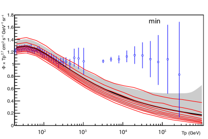
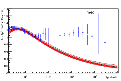
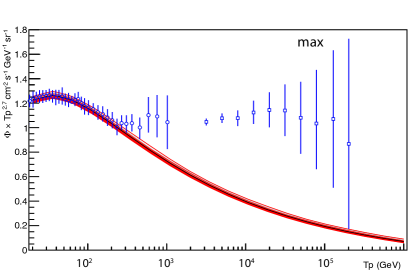
Figure 6: Confidence intervals for the flux from all the sources : the red curves show the 10 $\%$ quantiles, the black curves show the mean value and the grey band show the 68% confidence interval for the flux, for $\nu=3\;\text{century}^{-1}$.

5 Known local sources – The catalog

5.1 Regularization using a catalog

The situation described above occurs as long as we know nothing of the positions and ages of the CR sources. The young and nearby objects are responsible for the divergence of the flux variance and potentially lead to the problems encountered above in the statistical analysis. However, we actually have data concerning the distribution of nearby sources, for which catalogs are available. A natural way then to regularize the variance is to separate the sources in two lots. The first set contains the young and local sources, which can be extracted from the catalogs. The second group, on which little information is known, comprises the old or distant sources and will be treated according to the statistical analysis of Sec. 4. This procedure allows to regularize the variance of the flux in the most natural way while reducing its uncertainties. Following Delahaye et al. (2010), we have used two catalogs.

(i) The Green survey (Green 2009) compiles various informations on supernova remnants, but fails to systematically provide their ages or the precision with which their distances from the Earth have been determined. A quite thorough bibliographic work has been summarised in the appendix of Delahaye et al. (2010), which we have borrowed as a complement of the Green catalog. In total, we have collected 27 local SNR with their ages, distances from the Sun and, when possible, the corresponding observational uncertainties.

(ii) Pulsars are not expected to be sources of primary CR nuclei. As residues of supernova explosions, they are nevertheless a good tracer of old SNR too old to be detected directly in radio waves. Moreover, being point-like objects, their distances from the Sun is way easier to measure. Their ages can also be estimated precisely through spin-down. After removing millisecond pulsars from the ATNF catalog (Manchester et al. 2005) (by selecting $\dot{P}>5\times 10^{-18}$) and objects associated with known SNR, we are left with 157 objects with their ages and distances.

It is fair to ask whether these 27+157 sources are representative of the local environment. As featured in Fig. 7, the number of objects found in the catalogs is in good agreement with what can be inferred from various Galactic distributions found in the literature, provided that the supernova explosion rate is, on average, approximately equal to 3 per century. At least, this is true within the 2 kpc nearby the Sun, for sources younger than 30,000 years. At later ages, SNR become too dim to be detected and the Green survey cannot be trusted anymore. However, the catalogs are in rather good agreement with theoretical expectations and do not suffer from major biases, at least not more than the theoretical models. In this work, we define the “local” region as the domain extending 2 kpc around the Sun, with sources younger than 50,000 years. A rate of 1 supernova explosion per century in our Galaxy is also quoted in the literature (Delahaye et al. 2010). If so, we would be in a locally high-density region of sources. We have plotted the flux considering this low rate, but will discuss the validity of this assumption in a forthcoming letter.

The CR proton flux produced by the SNR and pulsars of our catalog is presented in Fig. 8, for the “min” CR propagation benchmark model. In the PAMELA energy region, the flux is dominated by pulsars whereas SNR come into play at the energies of CREAM.

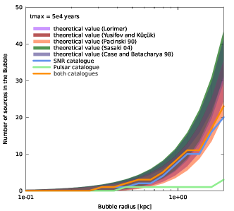
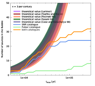
Figure 7: The bands indicate the theoretical expected number of sources within distance $r$ and for a given age (left), or with ages less than $t$ within a given distance (right), for a supernova rate of 3 explosions per century in the Galaxy. The width of the bands gauges the uncertainty in the number of local sources due to the shot-noise effect. The curves feature the cumulated number of sources in our catalog. This one appears to be complete for $t<5\times 10^{4}\;\text{y}$ and $r<2\;\text{kpc}$.

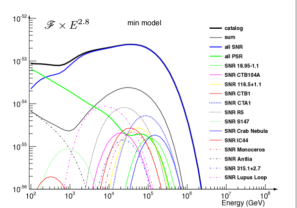
Figure 8: The CR proton flux is plotted as a function of energy for the SNR and pulsars which dominate over the other objects of our catalog.

5.2 Is the Catalog probable?

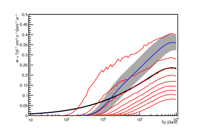
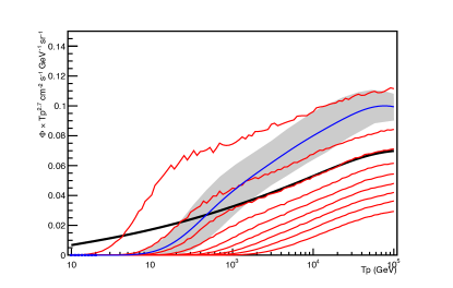
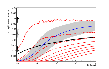
Figure 9: In each panel, the red lines correspond to the 10$\%$ quantiles of the CR proton flux generated by random sources drawn in the local region. The mean value is indicated by the black curve. The flux produced by the sources belonging to our catalog is represented in blue. The systematic errors associated to the uncertainties on the distances and ages of these objects span the grey band (standard deviation). All curves are derived with a supernova explosion rate of $\nu=3\;\text{century}^{-1}$. The min, med and max propagation benchmark models are considered.

In order to check the plausibility of our catalog, we compare in Fig. 9 the flux $\phi_{\rm cat}$ yielded by the sources which it contains (blue curve) to the flux $\phi_{\rm loc}$ from a set of populations drawn randomly inside the local region (black curve). As explained above, we did not compute the variance of these random populations, but derived through Monte-Carlo simulation the confidence intervals. Assuming an explosion rate of 3 events per century in the Galaxy, we find that the flux $\phi_{\rm cat}$ yielded by the objects of our catalog lies within the 1-$\sigma$ confidence interval surrounding the mean value $\phi_{\rm loc}$. This is true for the min, med and max benchmark sets of CR propagation parameters. We conclude that the theoretical source distribution and explosion rate, which we have chosen here, are in rather good agreement with local realistic sources. They are not necessarily representative of the entire Galaxy though. How potential differences would impact the relative importance of $\phi_{\rm cat}$ with respect to the total flux will be detailed in a forthcoming letter.

5.3 Systematic errors from the catalog

We have also plotted the uncertainty on $\phi_{\rm cat}$ that arises from the ages and positions of the SNR of our catalog. These have been varied within the ranges allowed by observations. We did not consider the uncertainties on the ages and positions of pulsars. The former are well determined. The rotation periods $P$ and drifts in time $\dot{P}$ of pulsars are actually measured with good accuracy. The uncertainty on $\phi_{\text{cat}}$ corresponds to the grey bands of Fig. 9 and Fig. 11. The shape of these curves is explained by the fact that when $L$ is lower (“min” model), the effective range of diffusion in the plane of the disk is reduced and the contribution of remote sources is smaller. The relative contribution of the catalog is then larger for smaller values of $L$.

6 A mixed approach

The cosmic ray flux from the Galactic sources and the associated uncertainties can be computed as

$$\phi_{\text{tot}}(E)=\phi_{\text{cat}}(E)+\phi_{\text{ext}}(E)$$

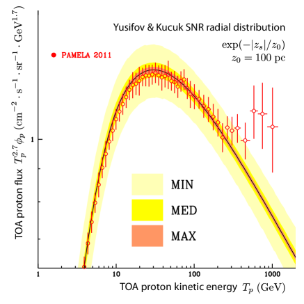
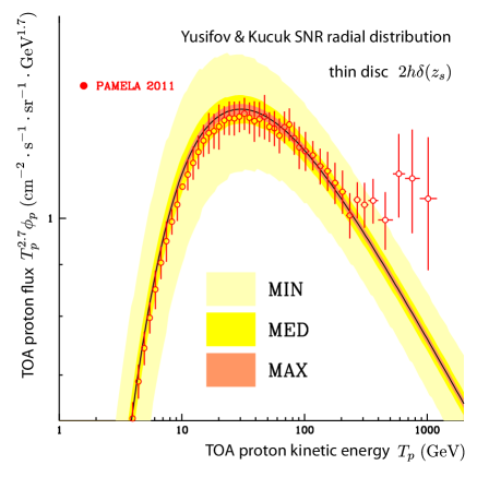
Figure 10: Mean flux (black curves) and envelopes representing the standard deviation of the flux, for the min, med and max propagation model and for an exponential distribution of sources along $z$ (left) and for a thin disk (right), for $\nu=3\;\text{century}^{-1}$.

where $\phi_{\text{cat}}$ is the flux coming from the sources belonging to the catalog (closer than 2 kpc and younger than $3\times 10^{5}$ yr) and $\phi_{\text{ext}}(E)$ is the flux coming from sources which are more distant than 2 kpc or older than $3\times 10^{5}$ yr. The uncertainties on $\phi_{\text{cat}}(E)$ are obtained by considering the observational errors on the source parameters (see Fig. 11). The uncertainty on $\phi_{\text{ext}}(E)$ can be evaluated by computing the confidence intervals, as above. In some conditions, this is equivalent to computing the usual the standard deviation of the flux, as the variance of the flux located outside of the region covered by the catalog is finite. This is shown in Fig. 10.

7 Conclusions

In the conventional model of Galactic CR propagation, the sources of primary nuclei are described as a jelly which spans the disk of the Milky Way and continuously injects particles inside the ISM. The actual distribution is lacunary and consists of point-like objects which release cosmic rays in a very short time. Because measurements have become very accurate, taking into account the discreteness of the sources in our description of CR propagation has become timely. In particular, the PAMELA (Adriani et al. 2011) and CREAM (Yoon et al. 2011) observations point towards an excess in the CR proton and helium fluxes with respect to the pure power-laws predicted with the continuous model. Very few analyses have been devoted so far to the myriad model. A challenging problem lies in the divergence of the variance of the CR primary flux. As shown recently by Blasi & Amato (2011), the second moment of the flux probability distribution function (PDF) is infinite. Although the variance can always be regularized in some way or another, this intriguing result threatens the conventional model of CR propagation, so far extremely successful. That is why we have thoroughly reinvestigated here how the discreteness of the sources may modify our vision of Galactic CR propagation.

To commence, the CR flux of primary cosmic rays obtained in the myriad model has a well-defined mean, identical to what is derived in the conventional approach by averaging the source distribution over space and time. This good point gives credit to the continuous model. We have then concentrated on the issue of the flux variance which diverges in the myriad model. Although the central limit theorem cannot be used in that case, at least in its ordinary form, the PDF of the flux is well defined everywhere inside the Galactic magnetic halo. We have run Monte Carlo simulations with several thousands of different populations of point-like sources. For the first time, we have derived the quantiles of the CR proton flux as a function of proton energy. The quantiles turn out to be well-defined and can be used to compute 68% confidence intervals. In spite of an infinite variance, meaningful error bars for the fluxes of primary CR nuclei can be defined. These depend on the propagation parameters and tend to decrease with the number of sources implied in the signal. That is why the uncertainty bands of Fig. 6 widen with the vertical extension $L$ of the CR diffusive halo.

We have so far focused on the flux at the Earth, but the same procedure can be applied throughout the Galaxy. It is however extremely time consuming and we defer to a subsequent publication the analytical derivation of the flux PDF. Such an investigation is crucial insofar as secondary species are produced by the interactions of primary CR nuclei on the ISM and the actual distribution of the latter matters. It would be interesting to examine the effect of the myriad hypothesis on the fluxes of antiprotons or positrons at the Earth as well as on the Galactic gamma ray diffuse emission. This emission has been so far calculated in the framework of the continuous model. An essential prediction is a gamma ray power law spectrum which traces the CR proton and helium energy distributions. According to the continuous hypothesis, we expect a gamma ray spectral index of $\sim-2.8\pm 0.1$ everywhere. Measurements by the H.E.S.S. collaboration (Aharonian et al. 2006) of the diffuse emission from the Galactic centre indicate a photon index of $2.29\pm 0.07\pm 0.02$, significantly below the prediction of the continuous model. Fluctuations of the CR proton and helium spectra around their mean values have thus already been observed.

As regards the primary CR fluxes at the Earth, another important result is the use of a catalog for the nearby and young sources which span the so-called local region. These objects have been extracted from the Green and ATNF surveys and are based on the latest astronomical observations. The catalog yields a contribution $\phi_{\rm cat}$ to the total flux $\phi$, whereas the sources extending beyond the local region contribute the complement $\phi_{\rm ext}$. This procedure provides a natural regularization of the flux variance since it is based on observations. We have found that below a few hundreds of GeV, $\phi_{\rm cat}$ is always negligible with respect to $\phi_{\rm ext}$, whatever the CR propagation parameters. Since the flux is dominated by distant or old sources, the continuous hypothesis applies and the use of the conventional CR propagation model is fully justified. We have succeeded in reconciling the myriad model with the continuous approach. Both should give identical results fo the low energy CR fluxes at the Earth. At the TeV scale and beyond, the situation becomes more complicated. If the total number of objects that source the flux is large with respect to the catalog, the contribution $\phi_{\rm ext}$ dominates and the continuous hypothesis is still valid at high energies. On the contrary, if the supernova explosion rate $\nu$ becomes smaller than the canonical value of 3 events per century, or if the half-thickness $L$ of the DH decreases, the catalog becomes relatively important and may even dominate the flux above a few TeV. This is actually the case for the black curve of Fig. 11 which corresponds to the min model and $\nu=1\;\text{century}^{-1}$. The CREAM data points lie inside the catalog 68% error band. Notice how well the CR proton excess is naturally explained by local and young sources which have actually been detected. There is no need for a break in the injection spectrum, nor for a peculiar behaviour of the diffusion coefficient $D$ with energy. It should even be possible to find a particuliar set of CR propagation parameters that would make the catalog a natural explanation of both PAMELA and CREAM data. Since the local region alone is implied, these parameters ought not to be the same as for the bulk of the Galactic magnetic halo.

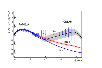
Figure 11: The blue, red and black curves feature the total flux $\phi$ computed as the sum of the mean external flux $\langle\phi_{\rm ext}\rangle$ and the contribution $\phi_{\rm cat}$ from the catalog. They respectively correspond to the max, med and min CR propagation benchmark models. The bands which extend around the curves have the same meaning as in Fig. 9. They indicate the standard deviation of the flux associated to the observational errors on the ages and distances of the SNR of the catalog.

Appendix A Computation of the Green function

In order to solve analytically Eq. (9), we need to simplify our description of the Milky Way DH and replace it by an infinite slab of half-thickness $L$ with a gaseous disk in the middle at $z=0$. Radial boundary conditions at $r=R_{\rm gal}$ are no longer implemented in the propagator. This simplification of the setup for CR propagation could be a problem if we were interested in the CR densities $\psi$ close to the radial boundaries, at a distance of 20 kpc from the Galactic center. But our aim is to calculate these densities at the Earth, at a galactocentric distance of $r_{\odot}=$ 8.5 kpc, i.e. far from the radial boundaries. Furthermore, even though the propagator $\mathscr{G}_{\!p}$ is derived within the framework of an infinite diffusive slab, integrals on the sources of cosmic rays, such as relation (7), are still performed up to the radial boundaries at $r=R_{\rm gal}$. We have checked that such a procedure does not introduce any significant error on the CR fluxes at the Earth. In the case of a source term $q_{\rm acc}$ that is continuous in space and time, this approach yields results very close to those obtained with a method based on radial Bessel functions. With this simplified setup, the propagation of CR species becomes invariant under a translation along the horizontal axes $x$ and $y$. The master equation (9) still needs to be solved along the vertical direction $z$, with the condition that $\mathscr{G}_{\!p}$ vanishes at the boundaries $z=\pm L$. The construction of the Green function for CR nuclei is inspired from the solution to the heat diffusion problem and has been given by many authors. The horizontal and vertical dependencies in $\mathscr{G}_{\!p}$ can be factored out by setting

$$\mathscr{G}_{\!p}\left(\mathbf{x},t\,\leftarrow\,\mathbf{x}_{S},t_{S}\right)={\displaystyle\frac{1}{4\pi D\tau}}\;\exp\left(-\,{\displaystyle\frac{\rho^{2}}{4D\tau}}\right)\;\mathscr{V}_{\!p}\left(z,t\,\leftarrow\,z_{S},t_{S}\right)\;\;,$$ (37)

where $\tau=t-t_{S}$ and $\rho^{2}=(x-x_{S})^{2}\,+\,(y-y_{S})^{2}$. The vertical function $\mathscr{V}_{\!p}$ is given by the expansion

$$\begin{split}\mathscr{V}_{p}&(z,t\,\leftarrow z_{S},t_{S})=\exp\left\{\frac{V_{C}\left(|z|-|z_{S}|\right)}{2D}\right\}\times\theta(\tau)\\ &\times\sum_{n=1}^{\infty}\left\{\frac{1}{C_{n}}\,e^{-\alpha_{n}\tau}\,\mathscr{E}_{n}(z)\,\mathscr{E}_{n}(z_{S})+\frac{1}{C^{\prime}_{n}}\,e^{-\alpha^{\prime}_{n}\tau}\,\mathscr{E}^{\prime}_{n}(z)\,\mathscr{E}^{\prime}_{n}(z_{S})\right\},\end{split}$$ (38)

where $\theta(\tau)$ is the Heaviside function. The sum runs over even and odd eigenfunctions. The former can be expressed as

$$\mathscr{E}_{n}(z)=\sin\left\{k_{n}(L-|z|)\right\}\;\;.$$ (39)

The corresponding even eigenwavevectors $k_{n}$ are solutions of the equation

$$-\,\tan(k_{n}L)={\displaystyle\frac{k_{n}}{k_{w}+k_{s}}}\;\;,$$ (40)

where $k_{w}\equiv{V_{C}}/{2D}$ and $k_{s}\equiv{h\Gamma_{p}}/{D}$ are typical wavevectors which account for the effects of Galactic convection and proton collisions on the ISM. Notice that at high energy, the dimensionless parameters $k_{w}L$ and $k_{s}L$ become very small as $D$ increases. We then expect convection and spallations to have little effect with respect to space diffusion at high energy, as illustrated in Fig. 12. The odd eigenfunctions are given by

$$\mathscr{E}^{\prime}_{n}(z)=\sin\left\{k^{\prime}_{n}(L-z)\right\}\;\;,$$ (41)

where the odd eigenwavevectors $k^{\prime}_{n}$ are such that $k^{\prime}_{n}L=n\pi$. This condition ensures that $\mathscr{E}^{\prime}_{n}(z)$ vanishes at $z=0$ and is an odd function of the height $z$. The decay rates $\alpha_{n}$ and $\alpha^{\prime}_{n}$ are respectively related to the eigenwavevectors $k_{n}$ and $k^{\prime}_{n}$ through

$$\alpha_{n}\,=\,Dk_{n}^{2}\,+\,{\displaystyle\frac{V_{C}^{2}}{4D}}\;\;.$$ (42)

$$\alpha_{n^{\prime}}\,=\,Dk_{n^{\prime}}^{2}\,+\,{\displaystyle\frac{V_{C}^{2}}{4D}}\;\;.$$

The eigenfunctions $\mathscr{E}_{n}(z)$ and $\mathscr{E}^{\prime}_{n}(z)$ may be understood as orthogonal vectors of a basis over which any vertical function that vanishes at $z=\pm L$ can be expanded. They are normalized in such a way that

$$\langle\mathscr{E}_{p}\,|\,\mathscr{E}_{n}\rangle\equiv{\displaystyle\int_{-L}^{+L}}\,dz\;\mathscr{E}^{\star}_{p}(z)\;\mathscr{E}_{n}(z)=\delta_{pn}\,C_{n}$$ (43)

and

$$\langle\mathscr{E}^{\prime}_{p}\,|\,\mathscr{E}^{\prime}_{n}\rangle=\delta_{pn}\,C^{\prime}_{n}\equiv\delta_{pn}\,L\;\;,$$ (44)

where the normalization factors $C_{n}$ and $C^{\prime}_{n}$ are

$$C_{n}=L\,\left\{1\,+\,{\displaystyle\frac{{\rm sinc}^{2}(k_{n}L)}{p}}\right\}\;\;\;{\rm and}\;\;\;C^{\prime}_{n}=L\;\;.$$ (45)

The dimensionless parameter $p$ is defined by ${1}/{p}=(k_{w}+k_{s})L$. It becomes infinite in the absence of Galactic convection and collisions on the ISM. In that limit, the eigenwavevectors $k_{n}$ are equal to ${(n-1/2)\,\pi}/{L}$.

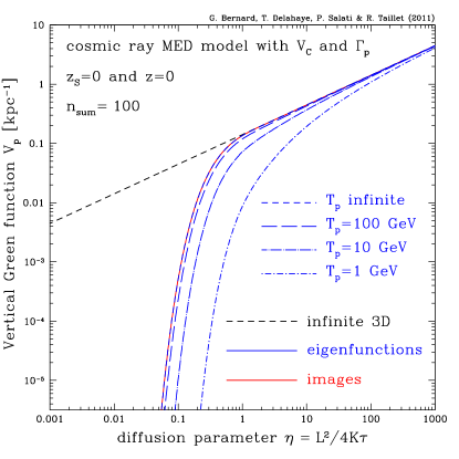
Figure 12: The effects of Galactic wind and spallations on the vertical propagator $\mathscr{V}_{\!p}$ are presented in this figure where the MED model of CR propagation, which best fits the B/C ratio, has been selected. At very high proton energy, diffusion dominates over the other processes and we recover the results obtained by setting $k_{w}$ and $k_{s}$ equal to 0. Because $n_{\rm sum}=100$ terms have been taken into account in the expansions (38) and (49), the blue short dashed curve matches exactly the red solid line. As the proton kinetic energy $T_{p}$ is decreased down to 1 GeV, Galactic convection and proton interactions on the ISM become more and more important and the blue curves departe from their infinite energy limit.

We still need to address a technical problem related to the behaviour of the vertical propagator (38) when $t$ is close to $t_{S}$. We shall find that the variance of the CR proton flux is dominated by local and recent supernova explosions. In that case, the period of time $\tau$ that separates the injection of protons from their detection at the Earth becomes small. The expansion (38) needs to be pushed a long way up in terms of the number of eigenfunctions involved. When $\tau$ is small, the exponentially decreasing functions $\exp(-\alpha_{n}\tau)$ and $\exp(-\alpha^{\prime}_{n}\tau)$ are still close to unity unless $n$ becomes very large. The numerical convergence of $\mathscr{V}_{\!p}$ requires then to sum expression (38) over an exceedingly large number of terms, hence a potential problem of CPU time. Because in that regime, most of the expansion (38) is provided by high order terms, Galactic convection and CR spallations become negligible with respect to diffusion. For these terms, the even eigenwavevectors $k_{n}$ are actually very close to their pure diffusion values of ${(n-1/2)\,\pi}/{L}$, even in the case where $p$ is not very large. In this regime of basically pure diffusion, another solution to CR propagation is provided by the method of electrical images. To commence, if the half-thickness $L$ of the slab is made infinite, we recover pure diffusion in infinite 3D space. In that case, the propagator is well-known, with a vertical contribution expressed as

$$\begin{split}\mathscr{V}_{\!p}\left(z,t\,\leftarrow\,z_{S},t_{S}\right)&\equiv\mathscr{V}_{\rm 1D}\left(z,t\,\leftarrow\,z_{S},t_{S}\right)\\ &=\frac{\theta(\tau)}{\sqrt{4\pi D\tau}}\,\exp\left\{-\frac{\left(z-z_{S}\right)^{2}}{4D\tau}\right\}\;\;.\end{split}$$ (46)

As already discussed by Baltz & Edsjö (1999), the vertical boundaries of the DH can now be implemented by associating to each point-like source lying at height $z_{S}$ the infinite series of its multiple images through the planes $z=\pm L$. The boundaries act as mirrors and give from the source an infinite series of images. The n-th image is located at

$$z_{n}\,=\,2L\,n\,+\,\left(-1\right)^{n}z_{S}\;\;,$$ (47)

and has a positive or negative contribution depending on whether $n$ is an even or odd number. When the diffusion time $\tau=t-t_{S}$ is small, the 1D solution (46) is a quite good approximation. The relevant parameter is actually

$$\eta\,=\,{\displaystyle\frac{L^{2}}{4D\tau}}\;\;,$$ (48)

and, in the regime where it is much larger than 1, i.e., for small values of $\tau$, the propagation is insensitive to the vertical boundaries. When the diffusion parameter $\eta$ decreases and the diffusion length $\lambda_{\rm D}\equiv\sqrt{4D\tau}$ becomes comparable to the half-thickness $L$ of the DH, images of the point-like source need to be taken into account in the sum

$$\mathscr{V}_{\!p}\left(z,t\,\leftarrow\,z_{S},t_{S}\right)\,=\,{\displaystyle\sum_{n\,=\,-\infty}^{+\infty}}\,\left(-1\right)^{n}\;\mathscr{V}_{\rm 1D}\left(z,t\,\leftarrow\,z_{n},t_{S}\right)\;\;.$$ (49)

When $\eta$ is much smaller than 1, many terms must be taken into account in the previous sum. However, this regime corresponds to large values of the diffusion time $\tau$ for which expansion (38) converges very rapidly.

We have devised two complementary methods to calculate the propagator $\mathscr{G}_{\!p}$. Depending on the value of the diffusion parameter $\eta$, we can use the relation (49) of electrical images ($\eta\geq 1$) or the expansion (38) ($\eta\leq 1$). Since the CR sources and the Earth are located inside the Galactic disk, we have set $z_{S}$ and $z$ equal to 0 in Fig. 12. The vertical part of the Green function depends only on the time delay $\tau=t-t_{S}$ with $\mathscr{V}_{\!p}(\tau)\equiv\mathscr{V}_{\!p}(0,t\,\leftarrow\,0,t_{S})=\mathscr{V}_{\!p}(0,\tau\,\leftarrow\,0,0)$. At low energy, Galactic convection and CR collisions on the ISM become important with respect to space diffusion. The method of electrical images is reliable only for small values of the diffusion time $\tau$. Expansion (49) can still be used to calculate $\mathscr{V}_{\!p}$ in the regime where $\eta$ becomes large. How large depends on the relative strength of the various CR propagation mechanisms. To get a flavor of the range of validity over which electrical images can be used even in the case where $k_{s}$ and $k_{w}$ are larger than ${1}/{L}$, we have borrowed the MED set of CR propagation parameters from Donato et al. (2004). This benchmark configuration provides the best fit to the B/C measurements (see Table 1). The black short dashed line of Fig. 12 corresponds to pure diffusion in infinite 3D space. The method of electrical images can only be used for pure CR diffusion and yields the red solid line. Expansion (49) has been calculated with $n_{\rm sum}=100$ images and is valid down to the small value of $\eta\sim 0.016$. Expansion (38) has also been pushed up to the 100-th term and converges even for $\eta$ as large as $10^{3}$. It leads to the blue curves which correspond each to a different proton kinetic energy $T_{p}$. Because diffusion takes over the other processes at very high energy, the blue short dashed curve is completely superimposed on the red solid line. In that regime, expansions (38) and (49) yield the same result. As $T_{p}$ decreases, convection and spallations come into play and the blue curves depart from their high energy limit. Notice that the 100 GeV configuration is still fairly close to the high energy case. At 10 GeV, the blue dotted-long dashed curve differs noticeably from the red solid line. The pure diffusive regime is nevertheless obtained for $\eta\geq 100$. Finally, the 1 GeV blue dotted-short dashed curve is significantly shifted towards higher values of $\eta$ with respect to the pure diffusive case. In order to reliably calculate the proton propagator below $\sim$ 1 GeV, many terms need to be taken into account in expansion (38). This sum should be used up to large values of $\eta$ before the electrical images provide an accurate result.

Appendix B Probability distribution for the flux

In this section, we compute the high-$\phi$ behaviour of the probability density $P(\phi)$ for the flux due to a point source drawn from a uniform spatial and temporal distribution. This high-$\phi$ tail of the distribution is the part leading to the divergence of the variance. It is due to the sources which are very close and very young, for which the effects of Galactic wind, escape and reacceleration are very small. We can neglect these effects, as long as we are only interested in the asymptotic behaviour of $P(\phi)$ at high $\phi$.

The flux at distance $r$ and at time $t$ from a point source emitting instantly all its particles at $r=0$ and $t=0$ is given by

$$\phi=\frac{a}{t^{3/2}}e^{-r^{2}/4Kt}\quad\text{where}\quad a=\frac{q}{(4\pi K)^{3/2}}$$

Case of a 2D distribution of sources (thin disk)

Let us first consider sources having a given age $t$. The probability density that a source lies at a distance $r$ is given by

$$p(r)\equiv\frac{dP(r)}{dr}=\frac{2r}{R^{2}}$$

where $R$ stands for the radius of the region containing the sources. We have

$$d\phi=-\frac{2r\,dr}{4Kt}\,\phi$$

so that

$$p(\phi|t)=\frac{dP(\phi,t)}{d\phi}=\frac{4Kt}{R^{2}}\,\frac{1}{\phi}$$

For an age $t$, fluxes are in the interval

$$\frac{a}{t^{3/2}}e^{-R^{2}/4Kt}\leq\phi\leq\frac{a}{t^{3/2}}$$

which can be written as

$$p(\phi|t)=\frac{4Kt}{R^{2}}\,\frac{1}{\phi}W\left(\frac{a}{t^{3/2}}e^{-R^{2}/4Kt},\frac{a}{t^{3/2}}\right)$$

Where $W$ stands for the window function, being equal to 1 in the interval and 0 outside. It is easily checked that

$$\int p(\phi|t)d\phi=\frac{4Kt}{R^{2}}\ln\frac{\phi_{\text{max}}}{\phi_{\text{min}}}=1$$

The probability distribution for $\phi$ is obtained by

$$p(\phi)=\int p(\phi|t)\,p(t)\,dt$$

where the upper bound is

$$t_{\text{max}}=a^{2/3}\phi^{-2/3}$$

the lower bound $t_{\text{min}}(\phi)$ is a solution of

$$\phi=\frac{a}{t_{\text{min}}^{3/2}}e^{-R^{2}/4Kt_{\text{min}}}$$

If the age distribution $p(t)$ is uniform between $0$ and $T$, we have $p(t)=1/T$ so that

$$p(\phi)=\frac{4K}{R^{2}T\phi}\int_{t_{\text{min}}}^{a^{2/3}\phi^{-2/3}}\,t\,dt$$

$$p(\phi)=\frac{2K}{R^{2}T\phi}\left[a^{4/3}\phi^{-4/3}-t_{\text{min}}^{2}(\phi)\right]$$

$$p(\phi)=\frac{2Ka^{4/3}}{R^{2}T}\left[\phi^{-7/3}-\frac{t_{\text{min}}^{2}(\phi)}{\phi a^{4/3}}\right]$$

This can be written as

$$p(\phi)=\frac{2Ka^{4/3}}{R^{2}T}\phi^{-7/3}\left[1-e^{-R^{2}/4Kt_{\text{min}}(\phi)}\right]$$

At high $\phi$, we have

$$p(\phi)\propto\phi^{-7/3}$$

Case of a 3D distribution of sources (thick disk)

If the sources are distributed in a volume instead of a surface, we still have

$$d\phi=-\frac{r\,dr}{2Kt}\,\phi$$

but

$$p(r)\equiv\frac{dP(r)}{dr}=\frac{3r^{2}}{R^{3}}$$

$$dP=\frac{3r^{2}dr}{R^{3}}=\frac{6rKt}{R^{3}}\frac{d\phi}{\phi}$$

As

$$r=\sqrt{-4Kt\ln(\phi t^{3/2}/a)}$$

we have

$$p(\phi|t)=\frac{12(Kt)^{3/2}}{R^{3}}\frac{\sqrt{-\ln(\phi t^{3/2}/a)}}{\phi}$$

As before, we can check that the total probability is 1. Let us compute

$$\int p(\phi|t)\,d\phi=\frac{12(Kt)^{3/2}}{R^{3}}\int\frac{\sqrt{-\ln(\phi t^{3/2}/a)}}{\phi}\,d\phi$$

We set $x=\phi t^{3/2}/a$,

$$\int p(\phi|t)\,d\phi=\frac{12(Kt)^{3/2}}{R^{3}}\int_{\phi_{\text{min}}t^{3/2}/a}^{\phi_{\text{max}}t^{3/2}/a}\frac{\sqrt{-\ln x}}{x}\,dx$$

The integral is given by

$$\int\frac{\sqrt{-\ln x}}{x}\,dx=\frac{2}{3}\left(-\ln x\right)^{3/2}+\text{cte}$$

so that

$$\int p(\phi|t)\,d\phi=\frac{8(Kt)^{3/2}}{R^{3}}\left[\left(-\ln x\right)^{3/2}\right]_{\phi_{\text{min}}t^{3/2}/a}^{\phi_{\text{max}}t^{3/2}/a}$$

Finally, as $\phi_{\text{max}}t^{3/2}=a$ and $\phi_{\text{min}}t^{3/2}=ae^{-R^{2}/4Kt}$,

$$\int p(\phi|t)\,d\phi=\frac{8(Kt)^{3/2}}{R^{3}}\left(\frac{R^{2}}{4Kt}\right)^{3/2}=1$$

The probability distribution is obtained by

$$p(\phi)=\int p(\phi|t)\,p(t)\,dt$$

As before, $p(t)=1/T$,

$$p(\phi)=\int\frac{12(Kt)^{3/2}}{TR^{3}}\frac{\sqrt{-\ln(\phi t^{3/2}/a)}}{\phi}dt$$

where the bounds $t_{\text{min}}$ and $t_{\text{max}}$ are the same as before. We define $y=t\phi^{2/3}/a^{2/3}$,

$$p(\phi)=\int\frac{12a^{5/3}(Ky)^{3/2}}{TR^{3}\phi}\frac{\sqrt{-\ln y^{3/2}}}{\phi}\frac{dy}{\phi^{2/3}}$$

$$p(\phi)=\frac{12a^{5/3}K^{3/2}}{TR^{3}\phi^{8/3}}\sqrt{\frac{3}{2}}\int y^{3/2}\sqrt{-\ln y}\,dy$$

with $y_{\text{max}}=1$ and $y_{\text{min}}(\phi)$ solution of $y=\exp(-R^{2}a\phi^{2/3}/6Ky)$. For high values of $\phi$, the lower bound vanishes and the integral does not depend on $\phi$, which yields the final result

$$p(\phi)\propto\phi^{-8/3}$$