IPMU12-0074

Enhancement of Proton Decay Rates
in Supersymmetric SU(5) Grand Unified Models

Junji Hisano^a,b, Daiki Kobayashi^a, and Natsumi Nagata^a,c

^aDepartment of Physics, Nagoya University, Nagoya 464-8602, Japan
^bIPMU, TODIAS, University of Tokyo, Kashiwa 277-8568, Japan
^cDepartment of Physics, University of Tokyo, Tokyo 113-0033, Japan

In the supersymmetric grand unified theories (SUSY GUTs), gauge bosons associated with the unified gauge group induce proton decay. We investigate the proton decay rate via the gauge bosons in the SUSY GUTs under the two situations; one is with extra vector-like multiplets, and the other is with heavy sfermions. It is found that the proton lifetime is significantly reduced in the former case, while in the latter case it is slightly prolonged. Determination of the particle contents and their mass spectrum below the GUT scale is important to predict the proton lifetime. The proton decay searches have started to access to the $10^{16}$ GeV scale.

1 Introduction

The grand unified theories (GUTs), which embed the Standard Model (SM) gauge group into a large single gauge group, are quite attractive, and so a variety of models of the theories are proposed since the earliest work based on the SU(5) symmetry group was presented by Georgi and Glashow in 1974 [1]. Among them, the supersymmetric grand unified theories (SUSY GUTs) are considered to be promising candidates since they realize the gauge coupling unification with great accuracy [2] as well as solving the hierarchy problem in the GUTs [3, 4]. The supersymmetric version of the Georgi-Glashow SU(5) GUT, which is the simplest among the SUSY GUTs, is called the Minimal SUSY SU(5) GUT [4].

One of the most distinctive features which GUTs predict is the existence of baryon-number violating interactions, such as proton decay. In the SUSY GUTs with $R$ parity, for example, proton decay is induced by two different processes: the colored-Higgs and the $X$-boson exchanging processes. The colored Higgs triplets are introduced for the Higgs doublets in the Minimal Supersymmetric Standard Model (MSSM) to be incorporated into the SU(5) multiplets. The colored-Higgs exchange yields baryon-number violating dimension-five operators, which give rise to the dominant contribution to proton decay in the Minimal SUSY SU(5) GUTs [5]. On the other hand, $X$ bosons are the gauge bosons in the unified SU(5) gauge group, and they induce proton decay through the dimension-six operators. Since there has been no experimental signal of proton decay so far, strong limits are imposed on these interactions, especially on the former one. Super-Kamiokande gives the bounds on the proton lifetime: $\tau(p\to e^{+}\pi^{0})>1.29\times 10^{34}$ yrs with 219.7 kt-yr of data [6] and $\tau(p\to K^{+}\bar{\nu})>3.3\times 10^{33}$ yrs with 172.8 kt-yr of data at 90% confidence level [7]. These bounds are so stringent that the Minimal SU(5) SUSY GUT is excluded since the colored-Higgs-boson exchange process yields too short lifetime in the $p\to K^{+}\bar{\nu}$ channel [8]. This prediction is, however, quite model-dependent. In fact, many models are proposed in order to allow them to evade the experimental constraints. Such attempts [9] are accomplished by pushing the mass of the colored Higgs much heavier than the GUT scale and/or suppressing the dimension-five operators by a certain symmetry, e.g., the Peccei-Quinn (PQ) symmetry [10] in the four-dimensional GUTs. In the extra-dimensional models, the $R$ symmetry is introduced to suppress the dimension-five proton decay [11]. With the extensions, the $X$-boson exchanging interactions become dominant and the proton lifetime turns out to be long enough to avoid the current limit. In this work, we assume such mechanism works and concentrate on the proton decay via the $X$-boson exchange.

Nowadays, the weak-scale supersymmetry itself is severely constrained by the experiments at the Large Hadron Collider (LHC). Since there has been no signal of SUSY particles, the ATLAS and the CMS collaborations give severe limits on their masses, especially those of colored particles [12]. Moreover, the collaborations have recently announced that they detected signatures of Higgs boson for the first time [13]. According to their results, the mass of Higgs boson is about 125 GeV. The result is welcome to the MSSM, which predicts the light Higgs boson, while the substantial radiative corrections are required in order to raise the mass of Higgs boson up to 125 GeV. Since the corrections are increased as the SUSY particles become heavy, this situation implies that the SUSY scale might be higher than the electroweak scale [14], and challenges natural solutions to the hierarchy problem. These results give constraints on models of the SUSY-breaking mediation. The low-energy gauge mediation model may be required to introduce several messenger multiplets so that the SUSY particles are heavy enough [15]. On the other hand, there have been several alternatives to explain the 125 GeV Higgs boson in an extension of the MSSM. Introducing vector-like supermultiplets to the MSSM is one of the simplest way to accomplish the purpose [16]. In this case, the quantum effects by the extra multiplets help to increase the Higgs-boson mass. With the multiplets being a representation of the grand unified group, the perturbative gauge coupling unification is still preserved with great accuracy.

The MSSM with vector-like multiplets and high-scale SUSY models modifies the proton decay rates. In this work, we examine it in detail. We will find that vector-like matters enhance the proton decay rate, while heavy sfermions extend its lifetime. This investigation indicates that the proton-decay experiments might provide a hint for the low-energy structure of the SUSY GUTs.

We assume that the SUSY GUTs are realized in the four-dimensional spacetime, and not consider the extra-dimensional SUSY GUTs in which the gauge symmetry is broken by the boundary conditions. In the latter models, the main decay modes of proton depend on configuration of quarks and leptons in the extra-dimensional space [17]. However, the decrease/enhancement of the proton lifetime we show are almost universal even in those models.

This paper is organized as follows. We begin by reviewing the SUSY SU(5) GUTs in Sec. 2, and discuss the proton decay via the $X$-boson exchange in the subsequent section. Then, we evaluate the lifetime of proton decay in the case of the MSSM with vector-like matters and heavy sfermions in Sec. 4 and Sec. 5, respectively. Section 6 is devoted to conclusion. In Appendix, we present formulae for evaluating the long-distance part of the renormalization factors.

2 SUSY SU(5) GUTs

First, we review the SUSY SU(5) GUTs in order to illustrate the notation and conventions which we use in this article. Just like the Georgi-Glashow SU(5) model [1], we assume that the SM fermions, as well as their superpartners, are embedded in a $\bar{\bf 5}\oplus{\bf 10}$ representation. The multiplets $\Phi$ and $\Psi$, which are the matter fields of $\bar{\bf 5}$ and ${\bf 10}$ representations, respectively, are identified as

$$\Phi =\begin{pmatrix}\bar{D}_{1}^{\prime}\\ \bar{D}_{2}^{\prime}\\ \bar{D}_{3}^{\prime}\\ E^{\prime}\\ -N^{\prime}\end{pmatrix}~{},~{}~{}~{}~{}~{}~{}\Psi=\frac{1}{\sqrt{2}}\begin{pmatrix}0&\bar{U}_{3}^{\prime}&-\bar{U}_{2}^{\prime}&U^{\prime 1}&D^{\prime 1}\\ -\bar{U}_{3}^{\prime}&0&\bar{U}_{1}^{\prime}&U^{\prime 2}&D^{\prime 2}\\ \bar{U}_{2}^{\prime}&-\bar{U}_{1}^{\prime}&0&U^{\prime 3}&D^{\prime 3}\\ -U^{\prime 1}&-U^{\prime 2}&-U^{\prime 3}&0&\bar{E}^{\prime}\\ -D^{\prime 1}&-D^{\prime 2}&-D^{\prime 3}&-\bar{E}^{\prime}&0\end{pmatrix}~{},$$ (1)

where all of the component fields are expressed in terms of the left-handed chiral superfields, and primes show that the above fields are the gauge eigenstates. The super/sub scripts of $U^{\prime\alpha}$, $D^{\prime\alpha}$, $\bar{U}_{\alpha}^{\prime}$, and $\bar{D}_{\alpha}^{\prime}$ denote a color index with $\alpha=1,2,3$. The chiral superfields $E^{\prime}$ and $N^{\prime}$ in $\Phi$ as well as $U^{\prime\alpha}$ and $D^{\prime\alpha}$ in $\Psi$ form the SU(2)_L doublets, respectively,

$$L^{\prime}=\begin{pmatrix}N^{\prime}\\ E^{\prime}\end{pmatrix}~{},~{}~{}~{}~{}~{}~{}Q^{\prime\alpha}=\begin{pmatrix}U^{\prime\alpha}\\ D^{\prime\alpha}\end{pmatrix}~{},$$ (2)

while $\bar{U}_{\alpha}^{\prime}$, $\bar{D}_{\alpha}^{\prime}$, and $\bar{E}^{\prime}$ are the SU(2)_L singlets.

The SU(5) gauge theory contains the 24 gauge bosons and each of them corresponds to a component of a vector superfield, ${\cal V}^{A}$, with $A=1,\dots,24$ indicating the gauge index. By exploiting the fundamental representation of the SU(5) generators, $T^{A}$, we define a $5\times 5$ matrix of the vector superfields: ${\cal V}\equiv{\cal V}^{A}T^{A}$. The components of the matrix are written as

$${\cal V}=\frac{1}{\sqrt{2}}\begin{pmatrix}\begin{matrix}G-\frac{2}{\sqrt{30}}B\end{matrix}&\begin{matrix}X^{\dagger 1}\\ X^{\dagger 2}\\ X^{\dagger 3}\end{matrix}&\begin{matrix}Y^{\dagger 1}\\ Y^{\dagger 2}\\ Y^{\dagger 3}\end{matrix}\\ \begin{matrix}X_{1}&X_{2}&X_{3}\\ Y_{1}&Y_{2}&Y_{3}\end{matrix}&\begin{matrix}\frac{1}{\sqrt{2}}W^{3}+\frac{3}{\sqrt{30}}B\\ W^{-}\end{matrix}&\begin{matrix}W^{+}\\ -\frac{1}{\sqrt{2}}W^{3}+\frac{3}{\sqrt{30}}B\end{matrix}\end{pmatrix}~{},$$ (3)

where each component is expressed by the same symbol as that used for the corresponding gauge field. We collectively refer to $X_{\alpha}$, $Y_{\alpha}$, and their Hermitian conjugates as $X$ and $Y$ bosons, and use the following notation for them:

$$(X)^{r}_{\alpha}=\begin{pmatrix}X^{1}_{\alpha}\\ X^{2}_{\alpha}\end{pmatrix}\equiv\begin{pmatrix}X_{\alpha}\\ Y_{\alpha}\end{pmatrix}~{}.$$ (4)

Here $r,s,\dots$ denote the isospin indices.

The Higgs superfields in the MSSM, on the other hand, are incorporated into a pair of fundamental and anti-fundamental fields as

$$H=\begin{pmatrix}H^{1}_{C}\\ H^{2}_{C}\\ H^{3}_{C}\\ H^{+}_{u}\\ H^{0}_{u}\end{pmatrix},~{}~{}~{}~{}~{}~{}\bar{H}=\begin{pmatrix}\bar{H}_{C1}\\ \bar{H}_{C2}\\ \bar{H}_{C3}\\ H^{-}_{d}\\ -H^{0}_{d}\end{pmatrix}~{},$$ (5)

where the last two components are corresponding to the MSSM Higgs superfields,

$$H_{u}=\begin{pmatrix}H^{+}_{u}\\ H^{0}_{u}\end{pmatrix},~{}~{}~{}~{}~{}~{}H_{d}=\begin{pmatrix}H^{0}_{d}\\ H^{-}_{d}\end{pmatrix}~{},$$ (6)

and the new Higgs superfields $H^{\alpha}_{C}$ and $\bar{H}_{C\alpha}$ are called the Higgs color triplet superfields. The superpotential for the Yukawa couplings of quarks and leptons is given as

$$W =\frac{1}{4}h^{ij}\epsilon_{abcde}\Psi_{i}^{ab}\Psi_{j}^{cd}H^{e}+\sqrt{2}f^{ij}\Psi_{i}^{ab}\Phi_{ja}\bar{H}_{b}~{},$$ (7)

where $i,j=1,2,3$ indicate the generations and $a,b,c,\dots$ represent the SU(5) indices. The Yukawa couplings $h^{ij}$ and $f^{ij}$ in Eq. (7) have redundant components and much of the degree of freedom is eliminated through the field re-definition of $\Psi$ and $\Phi$ [18]. We parametrize the couplings according to Ref. [19] as

$$h^{ij} =f_{u_{i}}e^{i\varphi_{i}}\delta_{ij}~{},$$ (8)

$$f^{ij} =V^{*}_{ij}f_{d_{j}}~{},$$ (9)

with $V_{ij}$ the Kobayashi-Maskawa matrix. The phase factors $\varphi_{i}$ are subject to a condition:

$$\varphi_{1}+\varphi_{2}+\varphi_{3}=0~{}.$$ (10)

With the parameters, we express the matter fields in terms of the mass eigenstates as follows:

$$Q^{\prime}_{i} =\begin{pmatrix}U_{i}\\ V_{ij}D_{j}\end{pmatrix},~{}~{}~{}~{}~{}~{}L_{i}^{\prime}=\begin{pmatrix}N_{i}\\ E_{i}\end{pmatrix},$$ (11)

$$\bar{U}_{i}^{\prime}=e^{-i\varphi_{i}}\bar{U}_{i},~{}~{}~{}~{}~{}~{}\bar{D}_{i}^{\prime}=\bar{D}_{i},~{}~{}~{}~{}~{}~{}\bar{E}_{i}^{\prime}=V_{ij}\bar{E}_{j}~{}.$$ (12)

In the following discussion, we express interactions in the basis of mass eigenstates unless otherwise noted.

Here, we do not take specific assumptions for symmetry breaking of SU(5) and the mass generation of the colored Higgs. They are related to suppression of the proton decay induced by dimension-five operators.

3 Proton decay via the $X$ and $Y$ boson exchange

Next we discuss the proton decay rate induced by the $X$ and $Y$ boson exchange. The couplings between the gauge bosons and the SM fermions are given as

$${\cal L}_{\rm int}=\frac{1}{\sqrt{2}}g_{5}\bigl{[}-\epsilon_{rs}(\overline{L^{\cal C}_{i}})^{r}{\ooalign{\hfil/\hfil\crcr$X$}}^{s}_{\alpha}P_{R}d^{\alpha}_{i} +\epsilon_{rs}V^{*}_{ij}\overline{e^{\cal C}_{j}}{\ooalign{\hfil/\hfil\crcr$X$}}^{r}_{\alpha}P_{L}Q^{\prime\alpha s}$$ (17)

$$+e^{-i\varphi_{i}}\epsilon^{\alpha\beta\gamma}(\overline{Q_{i}})_{\alpha r}{\ooalign{\hfil/\hfil\crcr$X$}}^{r}_{\beta}P_{L}(u^{\cal C}_{i})_{\gamma}+h.c.\bigr{]}~{},$$ (20)

where $g_{5}$ is the SU(5) gauge coupling constant and ${\cal C}$ indicates the charge conjugation. $\epsilon_{rs}$ and $\epsilon^{\alpha\beta\gamma}$ denote the second and third rank totally antisymmetric tensors, respectively. This interaction Lagrangian causes proton decay. In the present case, the dominant decay mode is $p\to\pi^{0}e^{+}$, and this decay process is induced by the following effective Lagrangian:

$${\cal L}_{\rm eff} =-\frac{g_{5}^{2}}{M_{X}^{2}}e^{i\varphi_{1}}\epsilon_{\alpha\beta\gamma}\bigl{[}A_{R}^{(1)}(\overline{u^{c}})^{\alpha}P_{R}d^{\beta}\overline{e^{+}}P_{L}u^{\gamma}+A^{(2)}_{R}(1+|V_{ud}|^{2})(\overline{u^{c}})^{\alpha}P_{L}d^{\beta}\overline{e^{+}}P_{R}u^{\gamma}\bigr{]}~{}.$$ (21)

where $M_{X}$ is the mass of $X$ and $Y$ bosons and $P_{L/R}\equiv\frac{1}{2}(1\mp\gamma_{5})$. The renormalization effects resulting from the anomalous dimensions of the operators are represented by $A_{R}^{(1)}$ and $A_{R}^{(2)}$, which we will evaluate below. The hadron matrix elements of the operators are evaluated by using the ordinary chiral Lagrangian method [22]:

$$\langle\pi^{0}|\epsilon_{\alpha\beta\gamma}[(\overline{u^{c}})^{\alpha}P_{R}d^{\beta}]P_{L}u^{\gamma}|p(\bm{p},s)\rangle=\frac{\alpha_{\rm H}}{\sqrt{2}f_{\pi}}(1+D+F)P_{L}u_{p}(\bm{p},s)~{},$$ (22)

and

$$\langle\pi^{0}|\epsilon_{\alpha\beta\gamma}[(\overline{u^{c}})^{\alpha}P_{L}d^{\beta}]P_{R}u^{\gamma}|p(\bm{p},s)\rangle=\frac{\alpha_{\rm H}}{\sqrt{2}f_{\pi}}(1+D+F)P_{R}u_{p}(\bm{p},s)~{},$$ (23)

where $f_{\pi}$ is the pion decay constant, and $\alpha_{\rm H}$ is defined by the equation

$$\langle 0|\epsilon_{\alpha\beta\gamma}[u^{\alpha}CP_{R}d^{\beta}]P_{L}u^{\gamma}|p(\bm{p},s)\rangle=\alpha_{\rm H}P_{L}u_{p}(\bm{p},s)~{},$$ (24)

with $C$ the charge conjugation matrix. The value of $\alpha_{\rm H}$ is computed in Ref. [23] as

$$\alpha_{\rm H}(2~{}{\rm GeV})=-0.0112\pm 0.0012_{(\rm stat)}\pm 0.0022_{(\rm syst)}~{}{\rm GeV}^{3},$$ (25)

at the renormalization scale $\mu=2$ GeV. By using the matrix elements, we obtain the partial decay width $\Gamma(p\rightarrow\pi^{0}e^{+})$ induced by the effective Lagrangian in Eq. (21):

$$\Gamma(p\rightarrow\pi^{0}e^{+})=\frac{\pi}{4}\frac{\alpha_{5}^{2}}{M_{X}^{4}}\frac{m_{p}}{f_{\pi}^{2}}\alpha_{\rm H}^{2}|1+D+F|^{2}\biggl{(}1-\frac{m_{\pi}^{2}}{m_{p}^{2}}\biggr{)}^{2}\bigl{[}\bigl{(}A^{(1)}_{R}\bigr{)}^{2}+\bigl{(}A^{(2)}_{R}\bigr{)}^{2}(1+|V_{ud}|^{2})^{2}\bigr{]}~{},$$ (26)

where $m_{p}$ and $m_{\pi}$ are the masses of proton and the neutral pion, respectively, and $\alpha_{5}\equiv g_{5}^{2}/4\pi$ . In the following calculation, we take $f_{\pi}=130~{}{\rm MeV}$, $D=0.80$, and $F=0.47$ as in Ref. [23].

Now, in order to evaluate the proton decay rate, all we have to do is to determine the unified gauge coupling constant $\alpha_{5}$, the $X$ boson mass $M_{X}$, and the renormalization factors $A^{(1)}_{R}$ and $A^{(2)}_{R}$. They are dependent on each GUT model.

The unified gauge coupling constant $\alpha_{5}$ is computed by solving the renormalization group equations (RGEs) for the gauge coupling constants $g_{a}$ ($a=1,2,3$) in the SM gauge interactions. In this article, we consider the gauge coupling running up to the two-loop level, and exploit the $\overline{\rm DR}$ renormalization scheme in order to respect the supersymmetry [24]. Furthermore, we adopt the definition of $\alpha_{5}$ as $\alpha_{5}\equiv g_{3}^{2}(M_{\rm GUT})/4\pi$ with $M_{\rm GUT}=1.5\times 10^{16}$ GeV.

In the MSSM, the two-loop renormalization group equations (RGEs) for the gauge coupling constants are given as [25]

$$\mu\frac{\partial g_{a}}{\partial\mu}=\frac{1}{16\pi^{2}}b_{a}^{(1)}g^{3}_{a}+\frac{g_{a}^{3}}{(16\pi^{2})^{2}}\biggl{[}\sum_{b=1}^{3}b_{ab}^{(2)}g_{b}^{2}-\sum_{i=t,b,\tau}c_{ai}~{}y^{2}_{i}\biggr{]}~{},$$ (27)

where

$$b^{(1)}_{a}=\begin{pmatrix}33/5\\ 1\\ -3\end{pmatrix}~{},~{}~{}~{}~{}b_{ab}^{(2)}=\begin{pmatrix}199/25&27/5&88/5\\ 9/5&25&24\\ 11/5&9&14\end{pmatrix}~{},~{}~{}~{}~{}~{}(a,b=1,2,3)$$ (28)

and

$$c_{ai}=\begin{pmatrix}26/5&14/5&18/5\\ 6&6&2\\ 4&4&0\end{pmatrix}~{},~{}~{}~{}~{}~{}~{}(i=t,b,\tau)$$ (29)

with $y_{i}$ the Yukawa couplings. Here, we use the SU(5) normalization for the U(1) hypercharge. Since the Yukawa couplings enter into the two-loop level contributions to the gauge coupling RGEs, it is sufficient to consider the RGEs for the Yukawa couplings at one-loop level. They are given as

$$\mu\frac{\partial}{\partial\mu}y_{t} =\frac{1}{16\pi^{2}}y_{t}\biggl{[}6y_{t}^{2}+y^{2}_{b}-\frac{13}{15}g^{2}_{1}-3g_{2}^{2}-\frac{16}{3}g_{3}^{2}\biggr{]},$$

$$\mu\frac{\partial}{\partial\mu}y_{b} =\frac{1}{16\pi^{2}}y_{b}\biggl{[}6y_{b}^{2}+y_{t}^{2}+y_{\tau}^{2}-\frac{7}{15}g^{2}_{1}-3g_{2}^{2}-\frac{16}{3}g_{3}^{2}\biggr{]},$$

$$\mu\frac{\partial}{\partial\mu}y_{\tau} =\frac{1}{16\pi^{2}}y_{\tau}\biggl{[}3y_{b}^{2}+4y_{\tau}^{2}-\frac{9}{5}g^{2}_{1}-3g_{2}^{2}\biggr{]}.$$ (30)

In the SM, on the other hand, the coefficients for the gauge coupling beta functions are [26]

$$b_{a}^{(1)}=\begin{pmatrix}41/10\\ -19/6\\ -7\end{pmatrix},~{}~{}~{}~{}~{}~{}b^{(2)}_{ab}=\begin{pmatrix}199/50&27/10&44/5\\ 9/10&35/6&12\\ 11/10&9/2&-26\end{pmatrix}~{},$$ (31)

and

$$c_{ai}=\begin{pmatrix}17/10&1/2&3/2\\ 3/2&3/2&1/2\\ 2&2&0\end{pmatrix}~{}.$$ (32)

The running of the Yukawa couplings in this case is given as follows:

$$\mu\frac{\partial}{\partial\mu}y_{t} =\frac{1}{16\pi^{2}}y_{t}\biggl{[}\frac{9}{2}y_{t}^{2}+\frac{3}{2}y_{b}^{2}+y_{\tau}^{2}-\frac{17}{20}g^{2}_{1}-\frac{9}{4}g_{2}^{2}-8g_{3}^{2}\biggr{]},$$

$$\mu\frac{\partial}{\partial\mu}y_{b} =\frac{1}{16\pi^{2}}y_{b}\biggl{[}\frac{3}{2}y_{t}^{2}+\frac{9}{2}y_{b}^{2}+y_{\tau}^{2}-\frac{1}{4}g^{2}_{1}-\frac{9}{4}g_{2}^{2}-8g_{3}^{2}\biggr{]},$$

$$\mu\frac{\partial}{\partial\mu}y_{\tau} =\frac{1}{16\pi^{2}}y_{\tau}\biggl{[}3y_{t}^{2}+3y_{b}^{2}+\frac{5}{2}y_{\tau}^{2}-\frac{9}{4}g^{2}_{1}-\frac{9}{4}g_{2}^{2}\biggr{]}.$$ (33)

Modifications in the coefficients in particular models are mentioned to in the following sections.

Now we deal with the renormalization factors, $A^{(1)}_{R}$ and $A^{(2)}_{R}$. The factors are expressed as the product of the long- and short-distance factors, i.e.,

$$A^{(i)}_{R}=A_{L}\cdot A_{S}^{(i)},~{}~{}~{}~{}~{}~{}(i=1,2)$$ (34)

where $A_{L}$ and $A_{S}^{(i)}$ represent the long- and short-distance factors, respectively. The long-distance contribution $A_{L}$ is common to $A_{R}^{(1)}$ and $A_{R}^{(2)}$, and independent of the high-energy physics. Its value is evaluated as

$$A_{L}=1.25~{},$$ (35)

at two-loop level. Details of the calculation are given in Appendix.

The short-distance factors are, on the other hand, model-dependent quantities. For instance, if there is no threshold between the electroweak and the GUT scales they are evaluated at one-loop level in Refs. [27, 28] as follows:

$$A_{S}^{(1)} =\biggl{[}\frac{\alpha_{3}(m_{Z})}{\alpha_{3}(M_{\rm GUT})}\biggr{]}^{-\frac{\gamma_{3}}{b_{3}^{(1)}}}\biggl{[}\frac{\alpha_{2}(m_{Z})}{\alpha_{2}(M_{\rm GUT})}\biggr{]}^{-\frac{\gamma_{2}}{b_{2}^{(1)}}}\biggl{[}\frac{\alpha_{1}(m_{Z})}{\alpha_{1}(M_{\rm GUT})}\biggr{]}^{-\frac{\gamma_{1}^{(1)}}{b_{1}^{(1)}}}~{},$$

$$A_{S}^{(2)} =\biggl{[}\frac{\alpha_{3}(m_{Z})}{\alpha_{3}(M_{\rm GUT})}\biggr{]}^{-\frac{\gamma_{3}}{b_{3}^{(1)}}}\biggl{[}\frac{\alpha_{2}(m_{Z})}{\alpha_{2}(M_{\rm GUT})}\biggr{]}^{-\frac{\gamma_{2}}{b_{2}^{(1)}}}\biggl{[}\frac{\alpha_{1}(m_{Z})}{\alpha_{1}(M_{\rm GUT})}\biggr{]}^{-\frac{\gamma_{1}^{(2)}}{b_{1}^{(1)}}}~{},$$ (36)

where, in the MSSM,

$$\gamma_{3}=\frac{4}{3},~{}~{}~{}~{}\gamma_{2}=\frac{3}{2},~{}~{}~{}~{}\gamma_{1}^{(1)}=\frac{11}{30},~{}~{}~{}~{}\gamma_{1}^{(2)}=\frac{23}{30}~{},$$ (37)

while in the SM,

$$\gamma_{3}=2,~{}~{}~{}~{}\gamma_{2}=\frac{9}{4},~{}~{}~{}~{}\gamma_{1}^{(1)}=\frac{11}{20},~{}~{}~{}~{}\gamma_{1}^{(2)}=\frac{23}{20}~{}.$$ (38)

The extension of the result to each case is referred to in the subsequent sections.

For reference, we evaluate the proton-decay lifetime assuming the SUSY scale to be 1 TeV, i.e., all the superparticles are assumed to have masses of ${\cal O}(1)$ TeV. The result is

$$\tau(p\to e^{+}\pi^{0})=1.16\times 10^{35}\times\biggl{(}\frac{M_{X}}{1.0\times 10^{16}~{}{\rm GeV}}\biggr{)}^{4}~{}~{}~{}~{}~{}{\rm years}~{}.$$ (39)

Here we neglect the possible effects of the threshold corrections from particles whose masses are around the GUT scale. We also neglect them in the following calculations, since the effects are completely model-dependent.

4 Proton decay with vector-like matters

In this section, we discuss the grand unified models in which extra vector-like matters are added into the SUSY SU(5) GUTs. We assume that there exist $n_{5}$ and $n_{10}$ pairs of chiral supermultiplets which transform as ${\bf 5}+\overline{\bf 5}$ and ${\bf 10}+\overline{\bf 10}$ representations, respectively, and evaluate the proton decay rate for the cases. For brevity, all of the multiplets are assumed to have the same mass, $M$. As mentioned to in the Introduction, such models are motivated by the symptoms of Higgs boson with its relatively heavy mass, $m_{h}\approx 125$ GeV, reported recently at the LHC [13]; if the additional multiplets with mass around weak scale couple to the MSSM Higgs bosons, the Higgs mass $m_{h}$ can be raised on account of the quantum corrections [16]. The gauge mediation requires the vector-like matters as the SUSY-breaking messenger. Thus, we take a wide parameter range for $M$.

The existence of the extra vector-like multiplets modifies the RGEs for the gauge coupling constants, as well as the short-distance renormalization factors. The beta functions of the gauge coupling constants in the MSSM receive additional contributions [29]:

$$\delta b^{(1)}_{a} =\begin{pmatrix}n_{5}+3n_{10}\\ n_{5}+3n_{10}\\ n_{5}+3n_{10}\end{pmatrix},$$

$$\delta b^{(2)}_{ab} =\begin{pmatrix}\frac{7}{15}n_{5}+\frac{23}{5}n_{10}&\frac{9}{5}n_{5}+\frac{3}{5}n_{10}&\frac{32}{15}n_{5}+\frac{48}{5}n_{10}\\ \\ \frac{3}{5}n_{5}+\frac{1}{5}n_{10}&7n_{5}+21n_{10}&16n_{10}\\ \\ \frac{4}{15}n_{5}+\frac{6}{5}n_{10}&6n_{10}&\frac{34}{3}n_{5}+34n_{10}\end{pmatrix}.$$ (40)

Here $\delta b^{(1)}_{a}$ and $\delta b^{(2)}_{ab}$ are the corrections to the leading and the next-to-leading order contributions for the beta functions of the gauge coupling constants, $b^{(1)}_{a}$ and $b^{(2)}_{ab}$, which are defined in Eq. (28). Here, we ignore the contribution from the Yukawa couplings of the vector-like matters at two-loop level for simplicity. From the one-loop contribution in Eq. (40), it is found that addition of vector-like matters equally changes the running of the gauge couplings, and thus maintains the gauge coupling unification.

The corrections to the one-loop contribution, $\delta b^{(1)}_{a}$, also modify $A_{S}^{(1)}$ and $A_{S}^{(2)}$. To be concrete, the renormalization effects of the energy scale above $M$ are given as

$$A_{S}^{(1)} =\biggl{[}\frac{\alpha_{3}(M)}{\alpha_{3}(M_{\rm GUT})}\biggr{]}^{-\frac{4}{3[b_{3}^{(1)}+\delta b_{3}^{(1)}]}}\biggl{[}\frac{\alpha_{2}(M)}{\alpha_{2}(M_{\rm GUT})}\biggr{]}^{-\frac{3}{2[b_{2}^{(1)}+\delta b_{2}^{(1)}]}}\biggl{[}\frac{\alpha_{1}(M)}{\alpha_{1}(M_{\rm GUT})}\biggr{]}^{-\frac{11}{30[b_{1}^{(1)}+\delta b_{1}^{(1)}]}}~{},$$

$$A_{S}^{(2)} =\biggl{[}\frac{\alpha_{3}(M)}{\alpha_{3}(M_{\rm GUT})}\biggr{]}^{-\frac{4}{3[b_{3}^{(1)}+\delta b_{3}^{(1)}]}}\biggl{[}\frac{\alpha_{2}(M)}{\alpha_{2}(M_{\rm GUT})}\biggr{]}^{-\frac{3}{2[b_{2}^{(1)}+\delta b_{2}^{(1)}]}}\biggl{[}\frac{\alpha_{1}(M)}{\alpha_{1}(M_{\rm GUT})}\biggr{]}^{-\frac{23}{30[b_{1}^{(1)}+\delta b_{1}^{(1)}]}}~{}.$$ (41)

These modifications result in alternations of the proton-decay lifetime. In order to parametrize the alternations, we define the following ratio:

$$R\equiv\frac{\tau(p\to e^{+}\pi^{0})|_{\rm w/}}{\tau(p\to e^{+}\pi^{0})|_{\rm w/o}}~{},$$ (42)

where $\tau(p\to e^{+}\pi^{0})|_{\rm w/(w/o)}$ represents the proton-decay lifetime with (without) vector-like matters. As seen form Eq. (26), this ratio does not depend on the $X$-boson mass but only on $\alpha_{5}$, $A_{S}^{(1)}$ and $A_{S}^{(2)}$:

$$R=\frac{\alpha_{5}^{2}\bigl{[}\bigl{(}A^{(1)}_{R}\bigr{)}^{2}+\bigl{(}A^{(2)}_{R}\bigr{)}^{2}(1+|V_{ud}|^{2})^{2}\bigr{]}_{\rm w/o}}{\alpha_{5}^{2}\bigl{[}\bigl{(}A^{(1)}_{R}\bigr{)}^{2}+\bigl{(}A^{(2)}_{R}\bigr{)}^{2}(1+|V_{ud}|^{2})^{2}\bigr{]}_{\rm w/}}~{}.$$ (43)

Here, w/ (w/o) again implies that the factor is for the case with (without) vector-like matters.

Figure 1: Ratio $R$ as functions of vector-like matter mass. Left and right graphs show $n_{5}=1,\dots,5$ and $n_{10}=1,\dots 3$ in solid lines from top to bottom, respectively. Light (dark) shaded region is excluded by the current experimental limit, $\tau(p\to e^{+}\pi^{0})>1.29\times 10^{34}$ years at 90% confidence level [6], in the case of $M_{X}=1.0\times 10^{16}$ GeV ($2.0\times 10^{16}$ GeV). SUSY scale is set to be 1 TeV.

In Fig. 1, we plot the ratio $R$ as functions of the masses of the vector-like multiplets. In the analysis, the SUSY scale is set to be $1$ TeV. Each solid line in the left graph corresponds to the number of ${\bf 5}+\overline{\bf 5}$ multiplets $n_{5}=1,2,\dots,5$ from top to bottom without ${\bf 10}+\overline{\bf 10}$ multiplets. In the right graph, on the other hand, the solid lines represent the cases with ${\bf 10}+\overline{\bf 10}$ multiplets ($n_{10}=1,2,3$, from top to bottom) and $n_{5}=0$. The light (dark) shaded region is excluded by the current experimental limit, $\tau(p\to e^{+}\pi^{0})>1.29\times 10^{34}$ years at 90% confidence level [6] in the case of $M_{X}=1.0\times 10^{16}$ GeV ($2.0\times 10^{16}$ GeV). On the whole parameter region in this figure, the unified gauge coupling constant, $\alpha_{5}$, is less than $0.6$, thus, perturbativity is maintained. In order to clarify the effects of the renormalization factors on the enhancement of proton decay rate, we also plot the ratio of the factors, $[(A^{(1)}_{R})^{2}+(A^{(2)}_{R})^{2}(1+|V_{ud}|^{2})^{2}]_{\rm w/}/[(A^{(1)}_{R})^{2}+(A^{(2)}_{R})^{2}(1+|V_{ud}|^{2})^{2}]_{\rm w/o}$, as functions of the masses of the vector-like multiplets in Fig. 2. Here we set $n_{5}=1,\dots,5$ from bottom to top and the SUSY scale to be 1 TeV. The renormalization factor in the absence of the vector-like multiplets is calculated as $[(A^{(1)}_{R})^{2}+(A^{(2)}_{R})^{2}(1+|V_{ud}|^{2})^{2}]_{\rm w/o}=40$ . These results indicate that the MSSM with vector-like matters might cause proton decay fast enough to be detected by the current or future experiments. In particular, if there are three ${\bf 5}+\overline{\bf 5}$ vector-like matters or is a ${\bf 10}+\overline{\bf 10}$ multiplet at the TeV scale, the SUSY SU(5) GUTs are excluded even by the present limit for $M_{X}=1.0\times 10^{16}$ GeV.

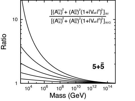
Figure 2: Enhancement of renormalization factors as functions of vector-like matter mass. We take $n_{5}=1,\dots,5$ from bottom to top. SUSY scale is set to be 1 TeV.

Figure 3: Ratio $R$ as functions of the masses of the multiplets. Solid lines represent $n_{g}=1,2$ multiplets of ${\bf 5}+\overline{\bf 5}+{\bf 10}+\overline{\bf 10}$ representations from top to bottom. Light (dark) shaded region is excluded by the current experimental limit, $\tau(p\to e^{+}\pi^{0})>1.29\times 10^{34}$ years at 90% confidence level [6] in the case of $M_{X}=1.0\times 10^{16}$ GeV ($2.0\times 10^{16}$ GeV). SUSY scale is set to be 1 TeV.

In addition, we calculate the ratio in the case where $n_{g}$ pairs of ${\bf 5}+\overline{\bf 5}+{\bf 10}+\overline{\bf 10}$ multiplets are introduced. This set of representations is the same as those of one generation of chiral matter fields and their corresponding complex representations. In this case, the beta functions are equal to those of $n_{5}=n_{10}=n_{g}$ in Eq. (40). After carrying out a similar calculation, we plot the ratio $R$ against the masses of the multiplets in Fig. 3. Here, solid lines represent $n_{g}=1,2$ multiplets of ${\bf 5}+\overline{\bf 5}+{\bf 10}+\overline{\bf 10}$ from top to bottom. We again set the SUSY scale to be 1 TeV. From this figure, it is found that a pair of extra generations which have masses below $10^{7}$ GeV yield too large proton decay rate to be excluded by the current experimental limit in the case of $M_{X}=1.0\times 10^{16}$ GeV. Although the threshold corrections around the GUT scale might alter the predicted values of proton lifetime, a growing tendency in the proton decay rate is independent of particular models. Therefore, the proton-decay experiments are extremely promising for constraining such scenario.

5 Proton decay with heavy SUSY particles

In turn, we discuss the SUSY GUT with sfermions having masses much larger than the TeV scale. Such a mass spectrum might be realized when the supersymmetry is broken via the anomaly-mediation mechanism [30], and there have been a lot of works which examine the scenario [31]. In this scenario, although a high degree of fine-tuning is inevitable, the SUSY flavor and CP problems are relaxed owing to heavy masses of sfermions [32]. The thermal relic scenario of dark matter in the Universe is still achieved [33], and the dark matter is to be directly detected in the future experiments [34]. In addition, this heavy scale SUSY scenario is also suggested by the recent LHC results since there has been no signal of superparticles and the ATLAS and CMS collaborations provide stringent limits on the masses of colored particles [12]. Moreover, in this case the SM-like Higgs boson mass easily reaches $\sim 125$ GeV as the radiative corrections are enhanced due to the heavy colored particles.

In the following discussion, we assume that the masses of squarks and sleptons are around the scale of $M_{\rm SF}$, which is much higher then the electroweak scale, while the masses of gauginos, higgsinos, and Higgs bosons except the lightest one are ${\cal O}(1)$ TeV, which is denoted by $M_{\rm GH}$ hereafter. Therefore, between $M_{\rm GH}$ and $M_{\rm SF}$, the latter fields are to be added to the RGE analysis. Furthermore, we assume that their contributions to the gauge-coupling running through the Yukawa couplings, as well as those with sfermions running in the loops, are negligible. Hence, the beta functions of the gauge couplings in this region are given as

$$b_{a}^{(1)}=\begin{pmatrix}23/5\\ -1\\ -5\end{pmatrix},~{}~{}~{}~{}~{}~{}b^{(2)}_{ab}=\begin{pmatrix}104/25&18/5&44/5\\ 6/5&32&12\\ 11/10&9/2&22\end{pmatrix}~{},$$ (44)

with $c_{ai}$ the same as the SM ones. Since each one-loop contribution $b^{(1)}_{a}$ in the above equation differ from that in Eq. (28) by the same number (2 in this case), the perturbative gauge coupling unification is again preserved in the present case.

Figure 4: Proton lifetime against $M_{\rm SF}$. Solid, dashed, and dotted lines correspond to the cases where $M_{\rm GH}$ is set to be 1, 3, and 10 TeV, respectively. $X$-boson mass is taken to be $1.0\times 10^{16}$ GeV.

In Fig. 4, we plot the lifetime of proton against $M_{\rm SF}$. Solid, dashed, and dotted lines correspond to the cases where $M_{\rm GH}$ is set to be 1, 3, and 10 TeV, respectively. The $X$-boson mass is taken to be $1.0\times 10^{16}$ GeV in this figure. It is found that the proton-decay lifetime is slightly extended , although the enhancement factor is less than two. The contribution of the renormalization factors to the alternation of the proton lifetime is less significant in this case than that in the case discussed in Sec. 4; It is at most a few % on the whole parameter region in this figure. Compared with the case discussed in the previous section, the present situation does not so much change the proton decay rate. Hence, searching for the proton decay is still stimulating even for the heavy SUSY scenario.

6 Conclusion

We have studied the proton decay rate under the two situations; one is the MSSM with vector-like multiplets, and the other is the MSSM with heavy sfermions. It is found that the proton lifetime is significantly reduced in the former case, while in the latter case it is slightly prolonged. In any case, the proton-decay experiments are, together with the LHC experiment and other precision measurements, expected to shed light on the supersymmetric grand unified models, as well as the supersymmetry itself.

Appendix: Long-distance part of the renormalization factors

In this Appendix, we demonstrate the evaluation of the long-distance contribution to the renormalization factors, e.g., $A_{L}$ in Eq. (34). First, we write down the two-loop renormalization group equations for the strong coupling constant below the electroweak scale:

$$\mu\frac{\partial g_{s}}{\partial\mu}=\frac{1}{16\pi^{2}}b_{1}g_{s}^{3}+\frac{1}{(16\pi^{2})^{2}}b_{2}g_{s}^{5}~{},$$ (45)

with $g_{s}$ the strong coupling constant and

$$b_{1}=-\biggl{(}11-\frac{2}{3}N_{f}\biggr{)},~{}~{}~{}~{}~{}b_{2}=-\biggl{(}102-\frac{38}{3}N_{f}\biggr{)}~{},$$ (46)

where $N_{f}$ denotes the number of quark flavors in an effective theory.

The long-distance factor, $A_{L}$, is determined by the ratio of the coefficients for the effective operators at the scale of $m_{Z}$ and 2 GeV:

$$A_{L}\equiv\frac{C(2~{}{\rm GeV})}{C(m_{Z})}~{},$$ (47)

with the coefficient $C(\mu)$ satisfying the following RGE at two-loop level [35]:

$$\mu\frac{\partial}{\partial\mu}C(\mu)=-\biggl{[}4\frac{\alpha_{s}}{4\pi}+\biggl{(}\frac{4}{3}+\frac{4}{9}N_{f}\biggr{)}\frac{\alpha_{s}^{2}}{(4\pi)^{2}}\biggr{]}C(\mu)~{}.$$ (48)

The solution of the equation is

$$\frac{C(\mu)}{C(\mu_{0})}=\biggl{[}\frac{\alpha_{s}(\mu)}{\alpha_{s}(\mu_{0})}\biggr{]}^{-\frac{2}{b_{1}}}\biggl{[}\frac{4\pi b_{1}+b_{2}\alpha_{s}(\mu)}{4\pi b_{1}+b_{2}\alpha_{s}(\mu_{0})}\biggr{]}^{\bigl{(}\frac{2}{b_{1}}-\frac{6+2N_{f}}{9b_{2}}\bigr{)}}~{},$$ (49)

with $b_{1}$ and $b_{2}$ given in Eq. (46). Thus, $A_{L}$ is given as

$$A_{L}=\biggl{[}\frac{\alpha_{s}(2~{}{\rm GeV})}{\alpha_{s}(m_{b})}\biggr{]}^{\frac{6}{25}}\biggl{[}\frac{\alpha_{s}(m_{b})}{\alpha_{s}(m_{Z})}\biggr{]}^{\frac{6}{23}}\biggl{[}\frac{\alpha_{s}(2~{}{\rm GeV})+\frac{50\pi}{77}}{\alpha_{s}(m_{b})+\frac{50\pi}{77}}\biggr{]}^{-\frac{173}{825}}\biggl{[}\frac{\alpha_{s}(m_{b})+\frac{23\pi}{29}}{\alpha_{s}(m_{Z})+\frac{23\pi}{29}}\biggr{]}^{-\frac{430}{2001}}~{},$$ (50)

and numerically it turns out to be

$$A_{L}=1.25~{}.$$ (51)

References

• [1] H. Georgi and S. L. Glashow, Phys. Rev. Lett.  32, 438 (1974).
• [2] S. Dimopoulos, S. Raby and F. Wilczek, Phys. Rev. D 24, 1681 (1981);
W. Marciano and G. Senjanović, Phys. Rev. D 25, 3092 (1982);
M.B. Einhorn and D.R. Jones, Nucl. Phys. B 196, 475 (1982);
U. Amaldi, W. de Boer and H. Furstenau, Phys. Lett. B 260, 447 (1991);
P. Langacker and M. -x. Luo, Phys. Rev. D 44, 817 (1991).
• [3] H. Georgi, H. R. Quinn and S. Weinberg, Phys. Rev. Lett.  33, 451 (1974);
S. Dimopoulos and S. Raby, Nucl. Phys. B 192, 353 (1981);
E. Witten, Nucl. Phys. B 188, 513 (1981).
• [4] S. Dimopoulos and H. Georgi, Nucl. Phys. B 193, 150 (1981);
N. Sakai, Z. Phys. C 11, 153 (1981).
• [5] N. Sakai and T. Yanagida, Nucl. Phys. B 197, 533 (1982);
S. Weinberg, Phys. Rev. D 26, 287 (1982).
• [6] H. Nishino, K. Abe, Y. Hayato, T. Iida, M. Ikeda, J. Kameda, Y. Koshio and M. Miura et al., arXiv:1203.4030 [hep-ex].
• [7] M. Miura, PoS ICHEP 2010, 408 (2010).
• [8] T. Goto and T. Nihei, Phys. Rev. D 59, 115009 (1999);
H. Murayama and A. Pierce, Phys. Rev. D 65, 055009 (2002) .
• [9] J. Hisano, H. Murayama and T. Yanagida, Phys. Lett. B 291, 263 (1992);
K. S. Babu and S. M. Barr, Phys. Rev. D 48, 5354 (1993);
J. Hisano, T. Moroi, K. Tobe and T. Yanagida, Phys. Lett. B 342, 138 (1995);
B. Bajc, P. Fileviez Perez and G. Senjanovic, Phys. Rev. D 66, 075005 (2002);
B. Bajc, P. Fileviez Perez and G. Senjanovic, hep-ph/0210374.
• [10] R. D. Peccei and H. R. Quinn, Phys. Rev. Lett.  38, 1440 (1977).
• [11] L. J. Hall and Y. Nomura, Phys. Rev. D 64, 055003 (2001) .
• [12] G. Aad et al. [ATLAS Collaboration], arXiv:1109.6572 [hep-ex];
S. Chatrchyan et al. [ CMS Collaboration ], [arXiv:1109.2352 [hep-ex]].
• [13] [ATLAS Collaboration], arXiv:1202.1408 [hep-ex];
S. Chatrchyan et al. [CMS Collaboration], arXiv:1202.1488 [hep-ex].
• [14] M. Ibe and T. T. Yanagida, Phys. Lett. B 709, 374 (2012);
M. Ibe, S. Matsumoto and T. T. Yanagida, Phys. Rev. D 85, 095011 (2012) .
• [15] M. A. Ajaib, I. Gogoladze, F. Nasir and Q. Shafi, arXiv:1204.2856 [hep-ph].
• [16] T. Moroi and Y. Okada, Phys. Lett. B 295, 73 (1992);
K. S. Babu, I. Gogoladze, M. U. Rehman and Q. Shafi, Phys. Rev. D 78, 055017 (2008);
S. P. Martin, Phys. Rev. D 81, 035004 (2010);
M. Asano, T. Moroi, R. Sato and T. T. Yanagida, Phys. Lett. B 705, 337 (2011);
M. Endo, K. Hamaguchi, S. Iwamoto and N. Yokozaki, Phys. Rev. D 84, 075017 (2011);
J. L. Evans, M. Ibe and T. T. Yanagida, arXiv:1108.3437 [hep-ph].
• [17] A. Hebecker and J. March-Russell, Phys. Lett. B 539, 119 (2002); L. J. Hall and Y. Nomura, Phys. Rev. D 66, 075004 (2002).
• [18] J. R. Ellis, M. K. Gaillard and D. V. Nanopoulos, Phys. Lett. B 80, 360 (1979) [Erratum-ibid.  82B, 464 (1979)] .
• [19] J. Hisano, H. Murayama and T. Yanagida, Nucl. Phys. B 402, 46 (1993) .
• [20] Y. Aoki, C. Dawson, J. Noaki and A. Soni, Phys. Rev. D 75, 014507 (2007) .
• [21] Y. Aoki, Talk at GUT2012, 16 March, 2012.
• [22] M. Claudson, M. B. Wise and L. J. Hall, Nucl. Phys. B 195, 297 (1982).
• [23] Y. Aoki et al. [RBC-UKQCD Collaboration], Phys. Rev. D 78, 054505 (2008) .
• [24] W. Siegel, Phys. Lett. B 84, 193 (1979).
• [25] J. E. Bjorkman and D. R. T. Jones, Nucl. Phys. B 259, 533 (1985).
• [26] M. E. Machacek and M. T. Vaughn, Nucl. Phys. B 222, 83 (1983).
• [27] L. F. Abbott and M. B. Wise, Phys. Rev. D 22, 2208 (1980).
• [28] C. Munoz, Phys. Lett. B 177, 55 (1986).
• [29] D. Ghilencea, M. Lanzagorta and G. G. Ross, Nucl. Phys. B 511, 3 (1998) .
• [30] L. Randall and R. Sundrum, Nucl. Phys. B 557, 79 (1999);
G. F. Giudice, M. A. Luty, H. Murayama and R. Rattazzi, JHEP 9812, 027 (1998) .
• [31] N. Arkani-Hamed and S. Dimopoulos, JHEP 0506, 073 (2005);
G. F. Giudice and A. Romanino, Nucl. Phys. B 699, 65 (2004) [Erratum-ibid. B 706, 65 (2005)];
N. Arkani-Hamed, S. Dimopoulos, G. F. Giudice and A. Romanino, Nucl. Phys. B 709, 3 (2005).
• [32] F. Gabbiani, E. Gabrielli, A. Masiero and L. Silvestrini, Nucl. Phys. B 477, 321 (1996) .
• [33] J. Hisano, S. Matsumoto, M. Nagai, O. Saito and M. Senami, Phys. Lett. B 646, 34 (2007) .
• [34] J. Hisano, K. Ishiwata and N. Nagata, Phys. Lett. B 690, 311 (2010);
J. Hisano, K. Ishiwata, N. Nagata and T. Takesako, JHEP 1107, 005 (2011);
T. Moroi and K. Nakayama, Phys. Lett. B 710, 159 (2012) .
• [35] T. Nihei and J. Arafune, Prog. Theor. Phys.  93, 665 (1995) .