Effect of disorder on the electronic properties of graphene: A theoretical approach

Abstract

In order to manipulate the properties of graphene, its very important to understand the electronic structure in presence of disorder. We investigate, within a tight-binding description, the effects of disorder in the on-site (diagonal disorder) term in the Hamiltonian as well as in the hopping integral (off-diagonal disorder) on the electronic dispersion and density of states by the augmented space recursion method. Extrinsic off-diagonal disorder is shown to have dramatic effects on the two-dimensional Dirac-cone, including asymmetries in the band structures as well as the presence of discontinuous bands (because of resonances) in certain limits. Disorder-induced broadening, related to the scattering length (or life-time) of Bloch electrons, is modified significantly with increasing strength of disorder. We propose that our methodology is suitable for the study of the effects of disorder in other 2D materials, such as a boron nitride mono layer.

I Introduction

Graphene, a two-dimensional allotrope of carbon, plays a central role in providing a basis for understanding the electronic properties of other carbon allotropes. Being one of the thinnest and the strongest material ever measured, graphene has attracted the attention of the materials research communityCastro09 in the recent past. One of the most interesting aspects of graphene is that its low energy dispersion closely resembles the Dirac spectrum of massless fermions. This particular type of dispersion provides a bridge between condensed matter physics and quantum electrodynamics (QED) for massless fermions. Of course in graphene, the Dirac fermions move with a much smaller speed.

Because of its unusual electronic and structural flexibility, properties of graphene can be controlled chemically or structurally in many different ways. For example, deposition of metal atomsCalandra07 on top of the graphene sheet, incorporating other elements like boron and nitrogenMartins07 randomly in the parent structure, either interstitially or substitutionally and using different substrates.Calizo07 Because disorder is unavoidable in any material, there has been an increasing interest in understanding how disorder affects the physics of electrons in graphene.uppsala Disordered graphene based derivatives can probably be referred to as functionalized graphene suitable for specific applications. “Graphene paper”Dikin07 is a spectacular example of how important such functionalization could be.

There can be many different sources of disorder in graphene including both intrinsic as well as extrinsic. Intrinsic sources may include surface ripples and topological defects. Extrinsic disorder comes in the form of vacancies, adatoms, quenched substitutional atoms and extended defects such as edges and cracks. Another way of introducing disorder is by ion-irradiation that produces complex defect structures in the graphene lattice.arkady Graphene in an amorphous form may increase the metallicity too.erik

To have a theoretical description of graphene’s electronic structure, one may begin with the Kohn-Sham equation and a tight-binding representation whose basis is labeled by the sites of the underlying Bravais lattice. Disorder may enter the matrix representation of the Hamiltonian in two ways : vacancies, dopants and adatoms predominantly cause a random change in the local single-site energy (disorder in the diagonal terms) but through the overlap such defects modify the hopping integrals between different sites (disorder in the off-diagonal terms) causing an effective random change in the distance or angle between the bonding orbitals. Thus diagonal and off-diagonal disorders simultaneously occur and are correlated. Model calculations which take them to be independent are qualitatively in error. As far as diagonal disorder is concerned, it acts as a simple chemical potential shift of the Dirac fermion i.e. shifts the Dirac point locally. Theoretical study of such disorder is rather simple and has indeed received attention and success, reported in literature.uppsala ^-35 A proper inclusion of off-diagonal disorder, on the other hand, is non-trivial and requires more sophisticated approaches.

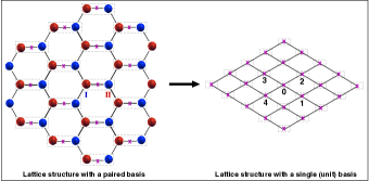
Figure 1: (Color online) (Left) The standard honeycomb lattice with a basis of two atoms per unit cell. (Right) The underlying rhombic Bravais lattice which becomes the honeycomb lattice when a pair of atoms decorate each site.

Figure 2: (Color Online) Nearest neighbor overlaps on the rhombic lattice

Till date there have been numerous attempts at studying the effects of disorder in graphene.uppsala ^-35 Among others, the methods used to study effects of disorder included the averaged t-matrix approximation (ATA)35 and the coherent potential approximation(CPA).CPA The first one is not self-consistent and hence inaccurate. The latter is a single-site mean field approximation with all its attendant problems.CPA Several others have used exact diagonalization of huge clusters and the real-space recursion of Haydock et al.35 ; hhk Both these techniques actually calculate the density of states (DOS) for specific configurations of the system followed by direct averaging over a large number of configurations. Since each of the configurations has periodic boundary conditions, the averaged spectral function is always a collection of delta functions and the disorder induced life-time effects cannot be probed. The recursion on the lattice probes mainly the real-space effects of disorder.

From the theoretical perspective, dealing with disorder has had a long history. As mentioned earlier, one of the most successful and frequently used approaches is the single-site, mean field CPA.CPA However, as the name itself suggests, it is a single site approximation and cannot adequately take into account the effects of correlated configuration fluctuations. In particular the CPA is inaccurate at low dimensions. In one dimension it is shown to be inadequate by Deandean some time ago. Among the hierarchy of the generalizations of CPA, only a few approaches have maintained the necessary Herglotz analytic properties and lattice translation symmetry of the configuration averaged Green’s function. These include the non-local CPA,NLCPA the special quasi-random structures (SQS),SQS the locally self-consistent multiple scattering approach (LSMS),LSMS and the three methods based on the augmented space formalism proposed by one of us Mookerjee73 : the traveling cluster approximation (TCA),TCA the itinerant coherent potential approximation (ICPA),ICPA and the augmented space recursion (ASR).ASR Over the years ASR has proved to be one of the most powerful techniques, which can accurately take into account the effects of correlated fluctuations arising out of the disorder in the local environment. This is reflected in a series of studies in the past e.g. the effects of local lattice distortion as in CuBe,Latt_dist short-range ordering due to local chemistry,SRO the phonon problem phonon with essential off-diagonal disorder in the dynamical matrices, and electrical and thermal transport propertiestransport in disordered alloys.

In this communication, we present a theoretical tight-binding model to study the effects of disorder in graphene. Disorders studied were mainly of two forms : substitutional disorder 10 ; 32 ^-34 and vacancies.4 ; 35 Unlike earlier models, both the diagonal and off-diagonal disorders are included on the same footing. The present formalism is based on the augmented space recursion.ASR Although recursion has been used to study graphene before, we want to emphasize that in all those applications recursion was carried out on a Hilbert space ${\cal H}$ spanned by the tight-binding basis representing the Hamiltonian. In augmented space recursion, we recurse in the space of all possible configurations which the Hamiltonian may assume in the disordered system. For a homogeneously disordered binary alloy, this configuration space is isomorphic to that of a spin-half Ising model. The augmented space theorem Mookerjee73 then connects configuration averages to a specific matrix element in that space of configurations.

The novel approach in this work is that we shall make use of the translation symmetries in augmented space (for homogeneous disorder) to carry out recursion in reciprocal space. This will directly give us the spectral function from which we extract the ’fuzzy’ band structure. The inclusion of the effects of configuration fluctuations of the immediate environment gives us self-energies which are strongly ${\bf k}$ dependent, unlike the CPA. In order to make a systematic study, we present results for combinations of both strong and weak diagonal and off-diagonal disorder. The combined effects show dramatic changes in the location and topology of the Dirac-like dispersion and the DOS. Special emphasis has been given to the non-trivial inclusion of off-diagonal disorder, in which case the averaged Bloch spectral function comes out to be significantly broadened, multiply peaked, and asymmetric in certain limits where the presence of resonances leads to discontinuous dispersion. The interesting interplay of the two kinds of disorder on full-widths at half maxima (FWHM) (related to the life-time of Bloch electrons in a disordered system) is also shown.

The rest of the paper is organized as follows. In Sec. II, we introduce the basic formalism. Sec. III is devoted to results and discussions. Concluding remarks are present in Sec. IV.

II Formalism

The most general tight-binding Hamiltonian for electrons in graphene can be represented as,

$$H=\sum_{R\alpha_{s}}\sum_{R^{\prime}\alpha_{s^{\prime}}}\left\{\epsilon_{R}^{\alpha_{s}}\delta_{RR^{\prime}}\delta_{ss^{\prime}}P_{R}^{\alpha_{s}}+V_{RR^{\prime}}^{\alpha_{s}\alpha_{s^{\prime}}}T_{RR^{\prime}}^{\alpha_{s}\alpha_{s^{\prime}}}\rule{0.0pt}{11.38109pt}\right\},$$ (1)

where $R,R^{\prime}$ denotes the position of the unit cell of the lattice, $\alpha_{s}$ denotes the $\alpha$-th atom on the $s$-th sublattice. The actual atomic position is $R+\zeta^{\alpha_{s}}$, where $\zeta^{\alpha_{s}}$ is the position of the $\alpha$-th atom on the $s$-th sublattice. $\epsilon_{R}^{\alpha_{s}}$ is the on-site energy describing the scattering properties of the atomic potential at $R+\zeta^{\alpha_{s}}$, and $V_{RR^{\prime}}^{\alpha_{s}\alpha_{s^{\prime}}}$ is the hopping integral between $R+\zeta^{\alpha}$ and $R^{\prime}+\zeta^{\alpha^{\prime}}$. $P$ and $T$ are the projection and transfer operators in the Hilbert space spanned by the tight-binding basis $|R\alpha_{s}\rangle$.

The above Hamiltonian $H$ describes electrons in the original honeycomb lattice of ion-cores, as shown in the left panel of Fig. 1. The two inequivalent sublattices (shown by red and blue spheres) are distinguished from each other. The underlying Bravais lattice is the rhombic lattice shown in the right panel of Fig. 1. Looking at Fig. 2 we can simplify Eqn.(1) further and write the Hamiltonian elements as $2\times 2$ matrices :

$$H=\sum_{R}\underline{\underline{\varepsilon}}_{R}\ P_{R}+\sum_{R\neq R^{\prime}}\underline{\underline{V}}_{RR^{\prime}}T_{RR^{\prime}},$$ (2)

where $\underline{\varepsilon}_{R}$ and $\underline{\underline{V}}_{RR^{\prime}}$, instead of being scalar for a single-band problem, are now $2\times 2$ matrices given by,

$$\underline{\underline{\varepsilon}}_{R}=\left(\begin{array}[]{cc}\varepsilon_{1}&t\\ t&\varepsilon_{2}\end{array}\right)\ \underline{\underline{V}}_{01}=\underline{\underline{V}}_{02}=\left(\begin{array}[]{cc}t^{\prime}&0\\ t&t^{\prime}\end{array}\right)$$ (7)

$$\underline{\underline{V}}_{03}=\underline{\underline{V}}_{04}=\left(\begin{array}[]{cc}t^{\prime}&t\\ 0&t^{\prime}\end{array}\right),$$ (10)

where $\varepsilon_{1}$ and $\varepsilon_{2}$ are the on-site energy on the two sublattices, $t$ and $t^{\prime}$ are the nearest neighbor and the next nearest neighbor hopping energies. $\underline{\underline{V}}_{0I}$ are the hopping matrices between the central site $0$ and its four neighboring sites $I$ (in the rhombic lattice) as shown in the right panel of Fig. 1. Because the next nearest neighbor hopping $t^{\prime}$ is usually very small compared to $t$, we shall treat the disorder effects only in the nearest neighbors.

For a system with substitutional disorder, the most general statement we can make is that the occupation of the lattice sites in each inequivalent sublattice can be different. For binary disorder in both the sublattices, we may introduce two random occupation variables $n_{R}^{I}$ and $n_{R}^{II}$ associated with the sublattices $I$ and $II$ such that,

$$n_{R}^{I}=\left\{\begin{array}[]{ll}1&\mbox{if $R\in A$ with probability x${}_{A}$ }\\ 0&\mbox{if $R\in B$ with probability x${}_{B}$ }\end{array}\right.$$

and

$$n_{R}^{II}=\left\{\begin{array}[]{ll}1&\mbox{if $R\in C$ with probability x${}_{C}$ }\\ 0&\mbox{if $R\in D$ with probability x${}_{D}$ }\end{array}\right.$$

where $A$, $B$ are the two types of atoms randomly occupying sublattice $I$ and $C$, $D$ are those occupying sublattice $II$.

The diagonal term $\underline{\varepsilon_{R}}$ for such a binary distribution can be written as,

$$\underline{\varepsilon}_{R} = \left(\begin{array}[]{cc}\epsilon_{A}^{I}&t_{AC}\\ t_{AC}&\epsilon_{C}^{II}\end{array}\right)n_{R}^{I}n_{R}^{II}+\left(\begin{array}[]{cc}\epsilon_{A}^{I}&t_{AD}\\ t_{AD}&\epsilon_{D}^{II}\end{array}\right)n_{R}^{I}(1-n_{R}^{II})+$$ (21)

$$\left(\begin{array}[]{cc}\epsilon_{B}^{I}&t_{BC}\\ t_{BC}&\epsilon_{C}^{II}\end{array}\right)(1-n_{R}^{I})n_{R}^{II}+$$

$$\left(\begin{array}[]{cc}\epsilon_{B}^{I}&t_{BD}\\ t_{BD}&\epsilon_{D}^{II}\end{array}\right)(1-n_{R}^{I})(1-n_{R}^{II})$$

$$= E_{1}+E_{2}\ n_{R}^{I}+E_{3}\ n_{R}^{II}+E_{4}\ n_{R}^{I}n_{R}^{II},$$ (22)

where

$$E_{1} = \left(\begin{array}[]{cc}\epsilon_{B}^{I}&t_{BD}\\ t_{BD}&\varepsilon_{B}^{II}\end{array}\right);\ \ \ E_{2}=\left(\begin{array}[]{cc}\delta\varepsilon_{1}&t^{(1)}\\ t^{(1)}&0\end{array}\right),$$ (27)

$$E_{3} = \left(\begin{array}[]{cc}0&t^{(2)}\\ t^{(2)}&\delta\varepsilon_{2}\end{array}\right);\ \ \ E_{4}=\left(\begin{array}[]{cc}0&t^{(3)}\\ t^{(3)}&0\end{array}\right)$$ (32)

with $\delta\varepsilon_{1}=\varepsilon^{I}_{A}-\varepsilon^{I}_{B}$; with $\delta\varepsilon_{2}=\varepsilon^{II}_{C}-\varepsilon^{II}_{D}$; $t^{(1)}=t_{AD}-t_{BD}$, $t^{(2)}=t_{BC}-t_{BD}$ and $t^{(3)}=t_{AC}+t_{BD}-t_{AD}-t_{BC}$.

Similarly the off-diagonal term $\underline{V}_{RR^{\prime}}$ in Eq. 10 can be expressed as (assuming $t^{\prime}=0$),

$$\underline{V}_{01}=\underline{V}_{02}=V_{1}+V_{2}\ n_{R}^{I}+V_{3}\ n_{R^{\prime}}^{II}+V_{4}\ n_{R}^{I}n_{R^{\prime}}^{II},$$ (33)

where

$$V_{1} = \left(\begin{array}[]{cc}0&0\\ t_{BD}&0\end{array}\right);\ \ \ V_{2}=\left(\begin{array}[]{cc}0&0\\ t^{(1)}&0\end{array}\right),$$ (38)

$$V_{3} = \left(\begin{array}[]{cc}0&0\\ t^{(2)}&0\end{array}\right);\ \ \ V_{4}=\left(\begin{array}[]{cc}0&0\\ t^{(3)}&0\end{array}\right).$$ (43)

$\underline{V}_{03}$ ($=\underline{V}_{04}$) are just the transpose of the above matrix $\underline{V}_{01}$. Various $t_{\alpha\beta}$’s in the above sets of equation are the hopping energies between various atom types ($\alpha=A,B$ and $\beta=C,D$) at two sublattices $I$ and $II$ respectively.

Next we proceed to calculate the configuration averaged Green function ( or the Bloch spectral function) in reciprocal space. We shall generalize the augmented space formalism (ASF) developed earlier in reciprocal space.kasr The ASF has been described in great detail earlier.Mook_book We shall indicate the main operational results here and refer the reader to the above monograph for further details. The first step is to associate with $n_{R}^{I}$ and $n_{R}^{II}$ two operators $N_{R}^{I}$ and $N_{R}^{II}$ such that their spectral density is the probability density of the random variables. For binary random variables, we have :

$$N_{R}^{I}=\left(\begin{array}[]{cc}x_{B}&\sqrt{x_{A}x_{B}}\\ \sqrt{x_{A}x_{B}}&x_{A}\end{array}\right)$$

Finally, according to augmented space theorem,Mookerjee73 the configuration average of any function of {$n_{R}^{I}$,$n_{R}^{II}$} can be written as the matrix element, in configuration space, of an operator which is the same functional of {$N_{R}^{I}$,$N_{R}^{II}$}. The augmented space Hamiltonian is built up from Eqns. (22) and (33).

$$\widehat{\mathbf{H}}=\sum_{R}\left\{E_{1}\widehat{I}+E_{2}\widetilde{N}^{I}_{R}+E_{3}\widetilde{N}^{II}_{R}+E_{4}\widetilde{N}^{I}_{R}\otimes\widetilde{N}^{II}_{R}\right\}\otimes P_{R}$$

$$+\sum_{R}\sum_{R^{\prime}}\left\{V_{1}\widehat{I}+V_{2}\widetilde{N}^{I}_{R}+V_{3}\widetilde{N}^{II}_{R^{\prime}}+V_{4}\widetilde{N}^{I}_{R}\otimes\widetilde{N}^{II}_{R^{\prime}}\right\}\otimes T_{RR^{\prime}}$$

with

$${N}_{R}^{X}=x_{\alpha}\ p_{R}^{X\uparrow}+x_{\beta}\ p_{R}^{X,\downarrow}+\sqrt{x_{\alpha}x_{\beta}}(\tau_{R}^{X,\uparrow\downarrow}+\tau_{R}^{X,\downarrow\uparrow}),$$ (44)

($X=I\ \text{or}\ II$)

Figure 3: Local density of states for pure graphene and graphene with a single impurity. The top panel in the middle is the DOS for pure graphene. Left and right panels show the local DOS with single impurity only on sublattice I or II and both I & II respectively. The panel from top to bottom are the results with increasing strength of the impurity potential $\delta{\text{E}}$=$\varepsilon_{\text{imp}}$-$\varepsilon_{\text{host}}$

Figure 4: Local density of states for graphene with a single vacancy. The vacancy site is modeled by a site with a large repulsive local potential. Technically we take $\delta{\text{E}}=\varepsilon_{\rm imp}-\varepsilon_{\rm host}$. The figures show consecutive situations with increasing $\delta\text{E}$ as we go from top to bottom.

The configuration averaged Green’s function in the reciprocal space is thus a matrix element of an augmented resolvent given by,

$$\ll G({\bf k},z)\gg=\langle\{\emptyset\}\otimes{\bf k}|(z\widehat{\bf I}-\widehat{\mathbf{H}})^{-1}|\ {\bf k}\otimes\{\emptyset\}\rangle,$$ (45)

$|\ {\bf k}\otimes\{\emptyset\}\rangle$ is an augmented space state in the reciprocal space given by,

$$|\ {\bf k}\otimes\{\emptyset\}\rangle=\frac{1}{\sqrt{N}}\sum_{R}e^{-i{\bf k.R}}|\ R\otimes\{\emptyset\}\rangle,$$ (46)

$|\ R\otimes\{\emptyset\}\rangle$ is an enlarged basis which is a direct product of the Hilbert space basis {$R$} and the configuration space basis $\{\phi_{R}\}$. The configuration space $\Phi=\prod_{R}^{\otimes}\phi_{R}$, takes care of the statistical average, is of rank $2^{M}$ for a system of $M$-lattice sites with binary distribution.

The recursion follows as a three step generation of a new basis $\{|n>\}$ :

$$|1\rangle=|{\bf k}\otimes\{\emptyset\}\rangle\qquad|0\rangle=0$$

$$|n+1\rangle=\widehat{H}|n\rangle-\alpha_{n}|n\rangle-\beta^{2}_{n-1}|n-1\rangle$$

$$\alpha_{n}({\bf k})=\frac{\langle n|\widehat{H}|n\rangle}{\langle n|n\rangle}\ \mbox{and }\ \beta_{n}^{2}(\bf k)=\frac{\langle n|n\rangle}{\langle n-1|n-1\rangle}$$

The ASR gives the configuration averaged spectral function as a continued fraction :

$$\ll G({\bf k},z)\gg = \frac{1}{\displaystyle z-\alpha_{1}({\bf k})-\frac{\beta_{1}^{2}({\bf k})}{\displaystyle z-\alpha_{2}({\bf k})-\frac{\beta_{1}^{2}({\bf k})}{z-\alpha_{3}({\bf k})-\frac{\ddots}{\displaystyle T(z,{\bf k})}}}}=\frac{1}{z-E_{0}({\bf k})-\Sigma(z,{\bf k})}$$ (47)

$T(z,{\bf k})$ is a continued fraction terminator as proposed by Beer and Pettifor.BF The spectral function peaks are decided by $\Re e\{\Sigma(E,{\bf k})\}$ and the imaginary part of $\Sigma$ gives the width related to the disorder induced lifetimes.

The configuration averaged Bloch spectral function is given by,

$$\ll A({\bf k},E)\gg=-\frac{1}{\pi}\lim_{\delta\rightarrow 0^{+}}\Im m\{\ll G({\bf k},E+i\delta)\gg\}$$ (48)

The configuration averaged density of states (DOS) is,

$$\ll n(E)\gg=\frac{1}{\Omega_{BZ}}\int_{BZ}d{\bf k}\ \ll A({\bf k},E)\gg$$ (49)

The electronic dispersion curves are obtained by numerically calculating the peak E-position of the spectral function. The full-widths at half maxima (FWHM) are also calculated from the disorder broadened Bloch spectral function.

III Results and Discussion

In the following subsections, we shall present our results for graphene with impurities, vacancies, diagonal disorder alone, and with the simultaneous presence of diagonal and off-diagonal disorder. The effects of various strengths of impurity potentials on two inequivalent sublattices will be shown via changes in the shape of the DOS. The changes in the topology of Dirac-cone dispersion, disorder-induced FWHM and the DOS will be shown for various strengths of diagonal disorder. In the most general case of diagonal and off-diagonal disorder, we consider three interesting limiting cases: (i) strong diagonal and weak off-diagonal disorder (ii) strong off-diagonal and weak diagonal disorder and (iii) strong diagonal as well as off-diagonal disorder. The interesting interplay between these different kinds of disorder in graphene reveals a discontinuous type of band near the $\Gamma$-point in the third limiting case.

Figure 5: (Color online) The averaged spectral functions (upper set of panels) and the complex bands (lower set of panels) near the Dirac point. These are all for pure diagonal disorder at three different alloy compositions (left to right) and four disorder strengths $\delta\text{E}$ (top to bottom). The (red) error bars show how the disorder induced lifetimes vary across the samples.

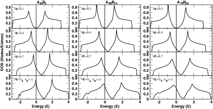
Figure 6: Total DOS for the same set of disorder strengths $\delta{\text{E}}$ for three alloys A${}_{x_{A}}$B${}_{x_{B}}$ as in Fig. 5. Due to homogeneous diagonal disorder on both the sublattices $I$ and $II$, the individual projected DOS on them are same in this case.

III.1 Impurities in Graphene

In Fig. 3, we display the DOS with different strengths of the single impurity potentials on different inequivalent sublattices. The top figure in the middle panel is the DOS for pure graphene. The left and right panels show local DOS with a single impurity put on the sublattice $I$ or $II$ and both respectively. The strength of the impurity potential (relative to the host lattice) increases from top to bottom panels (i.e. $\delta{\text{E}}$ = $\varepsilon_{\text{imp}}$ - $\varepsilon_{\text{host}}$ = $0.4$, $0.7$ and $1.0$). All these calculations are done with a fixed hopping parameter t=1. We notice changes in the shape of the hump and the van-Hove singularities as the strength of the impurity potential increases. Although the effects are small, but are clearly visible for the case of $\delta{\text{E}}$=1.0, where the local environment around the impurity site feels the strongest scattering. With the introduction of the impurity, the symmetry of the DOS around the Dirac point is lost. At these impurity levels, both the left and right panels show the formation of an impurity peak near the upper band edge. With increasing disorder this impurity peak moves into the band and disappears. Again, at these strengths there is no perceptible changes to the linear structure of the Dirac point. Similar results have been obtained previously for such models of impurities. This provides the correctness of our new formulation.

III.2 Single vacancies in graphene

An extension of the single impurity is the single vacancy in the model. The vacancy is modeled by a site with a large repulsive local potential. This is shown in Fig. 4. Notice that, with increasing $\delta\text{E}$, the rightmost impurity peak at around the top band-edge moves into the band. Most of the changes occur around the Dirac point at E=0. At $\delta\text{E}=2>t(=1)$ the symmetry of the Dirac point gets broken with the appearance of another mild peak. The origin of this ‘zero mode’ peak has been extensively discussed by Pereira et al.Pereira in detail. This peak grows with increasing disorder until at $\delta\text{E}\simeq 30$, where it takes the form of a delta function like structure at the Dirac point. The bottom panel shows the result for an ideal vacancy, where $t_{ij}=0$ for $t$ connecting the vacancy to the graphene lattice, or in other words a completely inaccessible ‘hard’ vacancy. The symmetry of the Dirac point is restored and the vacancy peak sits exactly at the Dirac point. This is exactly the same behavior reported by Pereira et al.Pereira who used either the CPA or direct real space recursion.

III.3 Diagonal disorder

Figure 7: (Color online) Same as Fig. 5, but with the inclusion of both diagonal and off-diagonal disorder. The three panels for each alloy indicate the results with coupled diagonal and off diagonal disorders as described in the text.

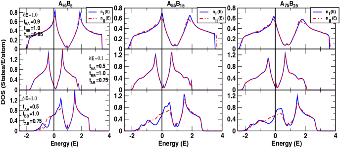
Figure 8: (Color online) Sublattice projected DOS for the same three set of diagonal+ off-diagonal disorder strengths for three alloys A${}_{x_{A}}$B${}_{x_{B}}$ as in Fig. 7. The projected DOS on the two sublattices n_I and n_II, in this case, are different due to the obvious reason arising from different random t_ij interactions.

First we shall take up purely diagonal disorder problems : those problems which can be taken up by earlier suggested methodologies. Of course, our augmented space recursion in reciprocal space give us additional information about the disorder induced life-times of the Bloch states. In Fig. 5, we display the configuration averaged Bloch spectral function (upper panels) (given by Eq. (48)) and the corresponding dispersion Energy vs. $k$ (lower panels) along $\Gamma-\text{K}-\Gamma$ symmetry line for three different alloys A${}_{x_{A}}$B${}_{x_{B}}$ ($x_{B}=5\%,15\%$ and $25\%$) with various diagonal disorder strengths. The two sublattices $I$ and $II$ are homogeneously disordered, such that $x_{A}=x_{C}$, $x_{B}=x_{D}$ and $\varepsilon_{A}^{I}=\varepsilon_{C}^{II}$, $\varepsilon_{B}^{I}=\varepsilon_{D}^{II}$. For each alloy case, the panels from top to bottom indicate the results with increasing strength of diagonal disorder (i.e. $\delta\text{E}$= $\varepsilon_{A}-\varepsilon_{B}$ = $0.1,0.4,0.7$ and $1.0$). The hopping integral $t$ is chosen to be 1 here, so there is no off-diagonal disorder. For each disorder strength $\delta\text{E}$ in a particular alloy, the upper panels show the averaged Bloch spectral function at five k-points along the high symmetry direction $\Gamma-$K. The corresponding Dirac dispersions are shown in the lower set of panels along $\Gamma-\text{K}-\Gamma$ line. The first thing to note is that the spectral function modifies quickly from sharp near $\delta$-functions to Lorentzian shapes with increasing disorder strength $\delta{\text{E}}$ as well as increasing alloy concentration $x_{B}$. In addition, the function gets more and more asymmetric with increasing $\delta{\text{E}}$. Such asymmetries can be described as a tendency of more scattering to occur near the resonance energies around $\Gamma$. In other words, line shapes around $\Gamma$ tend to have a weak second peak or wide tail over the resonance region. For the present diagonal disordered case, the Dirac point is simply shifted by an average energy $\langle\epsilon\rangle=x_{A}\epsilon_{A}^{I}+x_{B}\epsilon_{B}^{II}$

The corresponding total DOS for the same set of disorder strengths ($\delta\text{E}$) and the alloy concentrations ($x$) are shown in Fig. 6. The individual projected DOS on the two sublattices $I$ and $II$ in this case are same, because we have maintained uniform diagonal disorder on both the sublattices. However, the present theory is equally capable of treating the two sublattices differently with a different nature of disorder on them. In that case, the two inequivalent sublattices will have different projected quantities. Looking at Fig. 6, one can notice an exactly similar shift of the Dirac point (to the average $\langle\epsilon\rangle$) in the DOS as shown in the dispersion. The disorder effects are pronounced around the Dirac-point energy $\langle\epsilon\rangle$ and get milder around the hump below $\delta\text{E}=0.7$. Above this disorder strength, the left band edge starts to show up extra features with a dip at around $\text{E}=-2$, (as shown in the bottom panel for all the three alloy concentration). The results are qualitatively similar to the CPA works done earlierPereira but differ in quantitative details.

III.4 Off-diagonal disorder

We now turn to the cases with off-diagonal disorder. Such problems cannot be dealt with within the CPA. Also, direct calculation of the averaged spectral functions and disorder induced lifetimes is also not feasible with other techniques and the strength of the ASR comes to the fore. In addition we should note that in our model, diagonal and off-diagonal disorders are correlated : e.g. if the atom A occupies the site $i$ with probability $x_{A}$ and atom B occupies the site $j$ with probability $x_{B}$, then $t_{ij}$ has to be $t_{AB}$ with probability 1. Although the present theory is equally capable of investigating other interesting cases (e.g. inhomogeneous disorder, pseudo-binary type disorder etc.), here we have chosen to explore three cases which should reflect the behavior of a variety of the realistic materials. The three cases are:

• Strong diagonal and weak off-diagonal disorder; with parameters $\delta{\text{E}}=\epsilon_{A}^{I}-\epsilon_{B}^{I}=\epsilon_{C}^{II}-\epsilon_{D}^{II}=1.0$, $t_{AC}=1.0,t_{BD}=0.9$ and $t_{AD}=t_{BC}=0.95$.

• Weak diagonal and strong off-diagonal disorder; with parameters $\delta{\text{E}}=0.1$, $t_{AC}=1.0,t_{BD}=0.5$ and $t_{AD}=t_{BC}=0.75$.

• Strong diagonal as well as strong off-diagonal disorder; with parameters $\delta{\text{E}}=1.0$, $t_{AC}=1.0,t_{BD}=0.5$ and $t_{AD}=t_{BC}=0.75$.

The results for these three cases are shown in the top, middle and bottom panels of Fig. 7 respectively, for the same three alloys A${}_{x_{A}}$B${}_{x_{B}}$ as before. Other details are same as in Fig. 5. Notice that unlike the diagonal disordered case, effects of both diagonal and off-diagonal disorder are much more dramatic. In addition to highly asymmetric nature, the Bloch spectral function is found to have a double peaked structure in the extreme case of strong diagonal and off-diagonal disorder (shown in the bottom panels). Such doubly peaked line shape introduces extra discontinuous bands in the dispersion curve. Such a structure had been seen before in phonon problemsphonon which also have intrinsic off-diagonal disorder in the dynamical matrices. There it arose because of resonant modes. Here too we shall give a similar explanation. These dispersion at resonance have relatively large FWHM’s and it will be interesting to choose a realistic material of similar disorder properties and investigate the experimental outcome.

Figure 8 shows the sublattice projected DOS for the same three limiting cases for the three alloys as above. The solid blue and the dashed red lines indicate the projected DOS on the sublattices $I$ and $II$ respectively. Because of the random hopping (off-diagonal) interaction in this case, the two sublattices acquire different environment around it, and hence possess different projected quantities on them. As expected, the DOS in these cases have large smearing. The effective environment around the two sublattices is maximally different from each other in the extreme case of both strong diagonal+off-diagonal disorders (as shown in the bottom panels), as evident from the large difference between their projected DOS. Interestingly, for this particular case, the consequence of the discontinuous bands in the -ve energy range (bottom panels of Fig. 7) shows up via a dip in the DOS along with a much larger smearing. Apart from this extreme case, the Dirac point for all the other cases has moved in exact accordance with that of the band shift as in Fig. 7. The topology of the DOS on the two sides of the Dirac point are very different from each other specially in the case of strong diagonal and off-diagonal disorder (bottom panels). In totality, the effects of off-diagonal disorder is very different from that of diagonal disorder (as a comparison between Figs. 6 and 8 will show). Treatments of off-diagonal disorder is straight-forward and accurate in the ASR formalism.

IV Conclusion

We present a theoretical model to study the effects of diagonal and off-diagonal disorder in graphene on an equal footing. To our knowledge this is the first theoretical framework to reliably take into account the effects of off-diagonal disorder in describing the spectral properties of graphene. We show how the topology of the Dirac dispersion, and the location of Dirac point change with the strength of disorder and impurity concentration. Interestingly, the dispersion in case of strong diagonal and off-diagonal disorder tends to have an extra discontinuous band which is rather uncommon in the graphene fermiology with simple disorder. As such we propose to verify such effects in the electronic dispersion by setting up an experiment on a similar realistic graphene system, where both the diagonal and the off-diagonal disorder are strong. We believe that such a study may provide a deeper insight into the physics and materials perspective of graphene. Finally, we want to state that our formulation is quite general and can be applied to the case of other 2D materials, e.g., BN in presence of disorder.

Acknowledgments: AA acknowledges support from the U.S. Department of Energy BES/Materials Science and Engineering Division from contracts DEFG02-03ER46026 and Ames Laboratory (DE-AC02-07CH11358), operated by Iowa State University. This work was done under the HYDRA collaboration between the research groups..

References

- (1) A. H. Castro Neto, F. Guinea, N. M. R. Peres, K. S. Novoselov, and A. K. Geim, Rev. Mod. Phys. 81, 109 (2009).
- (2) M. Calandra and F. Mauri, Phys. Rev. B 76, 161406 (2007); Phys. Rev. B 76, 199901(E) (2007); B. Uchoa, C. -Y. Lin, and A. H. Castro Neto, Phys. Rev. B 77, 035420 (2008).
- (3) T. B. Martins, R. H. Miwa, A J. R. da Silva, and A. Fazzio, Phys. Rev. Lett. 98, 196803 (2007).
- (4) I. Calizo, W. Bao, F. Miao, C. N. Lau, and A. A. Balandin Appl. Phys. Lett 91, 201904 (2007); G. Giovannetti, P. A. Khomyakov, G. Brocks, P. J. Kelly, and J. van den Brink, Phys. Rev. B 76, 073103 (2007).
- (5) V. A. Coleman, R. Knut, O. Karis, H. Grennberg, U.Jansson, R. Quinlan and B. C. Holloway, B. Sanyal and O. Eriksson, J. Phys. D: Appl. Phys. 41, 062001(2008); S. H. M. Jafri, K. Carva, E. Widenkvist, T. Blom, B. Sanyal, J. Fransson, O. Eriksson, U. Jansson, H. Grennberg, O. Karis, R. A. Quinlan, B. C. Holloway, and K. Leifer, J. Phys. D: Appl. Phys. 43, 045404 (2010); K. Carva, B. Sanyal, J. Fransson, and O. Eriksson, Phys. Rev. B 81, 245405 (2010).
- (6) D. A. Dikin et al., Nature 448, 457 (2007); J. T. Robinson et al., Nano Lett 8, 3441 (2008).
- (7) F. Banhart, J. Kotakoski and A. V. Krasheninnikov, ACS Nano 5, 26 (2011).
- (8) E. Holmström, J. Fransson, O. Eriksson, R. Lizarraga, B. Sanyal, S. Bhandary, and M. I. Katsnelson, Phys. Rev. B 84, 205414 (2011).
- (9) Shangduan Wu, Lei Jing, Qunxiang Li, Q. W. Shi, Jie Chen, Haibin Su, Xiaoping Wang, and Jinlong Yang, Phys. Rev. B 77, 195411 (2008)
- (10) P. Soven, Phys. Rev. 156, 809 (1967); G. M. Stocks, W. M. Temmerman, and B. L. Gyorffy, Phys. Rev. Lett. 41, 339 (1978).
- (11) R. Haydock, V. Heine and M. J. Kelly, J. Phys. C: Solid State Phys 5, 2845 (1975).
- (12) P. Dean, Rev. Mod. Phys. 44, 127-168 (1972).
- (13) D. A. Biava1, Subhradip Ghosh, D. D. Johnson, W. A. Shelton, and A. V. Smirnov, Phys. Rev. B 72, 113105 (2005); Derwyn A. Rowlands, Julie B. Staunton, Balazs L. Györffy, Ezio Bruno, and Beniamino Ginatempo, Phys. Rev. B 72, 045101 (2005).
- (14) A. Zunger, S. -H. Wei, L. G. Ferreira and J. E. Bernard, Phys. Rev. Lett. 65, 353 (1990).
- (15) Y. Wang, G. M. Stocks, W. A. Shelton, D. M. C. Nicholson, Z. Szotek, and W. M. Temmerman, Phys. Rev. Lett. 75, 2867 (1995).
- (16) Abhijit Mookerjee, J. Phys. C: Solid State Phys 6, L205 (1973).
- (17) R. Mills and P. Ratanavararaksa, Phys. Rev. B 18, 5291 (1978); T. Kaplan, P. L. Leath, L. J. Gray, and H. W. Diehl, Phys. Rev. B 21, 4230 (1980).
- (18) S. Ghosh, P. L. Leath and M. H. Cohen, Phys. Rev. B 66, 214206 (2002).
- (19) T. Saha, I. Dasgupta, and A. Mookerjee, J. Phys.: Condens. Matter 6, L245 (1994).
- (20) T. Saha and A. Mookerjee, J. Phys.: Condens. Matter 8, 2915 (1996).
- (21) A. Alam and A. Mookerjee, J. Phys.: Condens. Matter 21, 195503 (2009); T.Saha, I. Dasgupta, and A. Mookerjee, Phys. Rev. B 50, 13267 (1994).
- (22) A. Alam, S. Ghosh, and A. Mookerjee, Phys. Rev. B 75, 134202 (2007); A. Alam and A. Mookerjee, Phys. Rev. B 69, 024205 (2004).
- (23) A. Alam and A. Mookerjee, Phys. Rev. B 72, 214207 (2005); K. Tarafder, A. Chakrabarti, K. K. Saha and A. Mookerjee, Phys. Rev. B 74, 144204 (2006).
- (24) K. Nomura and A. H. MacDonald, Phys. Rev. Lett. 98, 076602 (2007)
- (25) Y. V. Skrypnyk and V. M. Loktev, Phys. Rev. B 75, 245401 (2007)
- (26) T. O. Wehling, A. V. Balatsky, M. I. Katsnelson, A. I. Lichtenstein, K. Scharnberg and R. Wiesendanger, Phys. Rev. B 75, 125425 (2007)
- (27) N. M. R. Peres, F. Guinea and A. H. Castro Neto, Phys. Rev. B 73, 125411 (2006)
- (28) P. Biswas, B. Sanyal, M. Fakhruddin, A. Halder, A. Mookerjee and M. Ahmed, J. Phys.:Condens. Mat. 7, 8569 (1995).
- (29) A. Mookerjee, Electronic Structure of Alloys, Surfaces and Clusters (ed. D.D. Sarma and A. Mookerjee) (Taylor Francis, London) (2003).
- (30) N. Beer and D.G. Pettifor, Electronic Structure of Complex Systems ed. P. Phariseau and W. M. Temmerman (Plenum, New York, 1984) p 769.
- (31) Vitor M. Pereira, F. Guinea, J. M. B. Lopes dos Santos, N. M. R. Peres and A. H. Castro Neto, Phys. Rev. Lett. 96, 036801 (2006); Vitor M. Pereira, J. M. B. Lopes dos Santos and A. H. Castro Neto, Phys. Rev. B 77, 115109 (2008).