Geometric Separation by
Single-Pass Alternating Thresholding

Abstract.

Modern data is customarily of multimodal nature, and analysis tasks typically require separation into the single components. Although a highly ill-posed problem, the morphological difference of these components sometimes allow a very precise separation such as, for instance, in neurobiological imaging a separation into spines (pointlike structures) and dendrites (curvilinear structures). Recently, applied harmonic analysis introduced powerful methodologies to achieve this task, exploiting specifically designed representation systems in which the components are sparsely representable, combined with either performing $\ell_{1}$ minimization or thresholding on the combined dictionary.

In this paper we provide a thorough theoretical study of the separation of a distributional model situation of point- and curvilinear singularities exploiting a surprisingly simple single-pass alternating thresholding method applied to the two complementary frames: wavelets and curvelets. Utilizing the fact that the coefficients are clustered geometrically, thereby exhibiting clustered/geometric sparsity in the chosen frames, we prove that at sufficiently fine scales arbitrarily precise separation is possible. Even more surprising, it turns out that the thresholding index sets converge to the wavefront sets of the point- and curvilinear singularities in phase space and that those wavefront sets are perfectly separated by the thresholding procedure. Main ingredients of our analysis are the novel notion of cluster coherence and clustered/geometric sparsity as well as a microlocal analysis viewpoint.

1. Introduction

Along with the deluge of data we face today, it is not surprising that the complexity of such data is also increasing. One instance of this phenomenon is the occurrence of multiple components, and hence, analyzing such data typically involves a separation step. One most intriguing example comes from neurobiological imaging, where images of neurons from Alzheimer infected brains are studied with the hope to detect specific artifacts of this disease. The prominent parts of images of neurons are spines (pointlike structures) and dendrites (curvelike structures), which require separate analyzes, for instance, counting the number of spines of a particular shape, and determining the thickness of dendrites [31, 34].

From an educated viewpoint, it seems almost impossible to extract two images out of one image; the only possible attack point being the morphological difference of the components. The new paradigm of sparsity, which has lately led to some spectacular successes in solving such underdetermined systems, does provide a powerful means to explore this difference. The main sparsity-based approach towards solving such separation problems consists in carefully selecting two representation systems, each one providing a sparse representation of one of the components and both being incoherent with respect to the other – the encoding of the morphological difference –, followed by a procedure which generates a sparse expansion in the dictionary combining the two representation systems. This intuitively automatically forces the different components into the coefficients of the ‘correct’ representation system.

Browsing through the literature, the two main sparsity-based separation procedures can be identified to be $\ell_{1}$ minimization (see, e.g., [2, 15, 16, 17, 19, 20, 21, 22, 23, 27, 36, 37, 38, 40]) and thresholding (see, e.g., [1, 21, 32, 33]). For general papers on $\ell_{1}$ minimization techniques we refer to [7, 9, 14, 13, 12] and thresholding to [39] or the reference list in the beautiful survey paper [3]. While $\ell_{1}$ minimization has produced very strong theoretical results, thresholding is typically significantly harder to analyze due to its iterative nature. However, thresholding algorithms are in general much faster than $\ell_{1}$ minimization, which makes them particularly attractive for the aforementioned neurobiological imaging application due to its large problem size.

In this paper we focus on thresholding as a separation technique for separating point- from curvelike structures using radial wavelets and curvelets; in fact, we study the very simple technique of single-pass alternating thresholding, which expands the image in wavelets, thresholds and reconstructs the point part, then expands the residual in curvelets, thresholds and reconstructs the curve part. In this paper we aim for a fundamental mathematical understanding of the precision of separation allowed by this thresholding method. Interestingly, our analysis requires the notions of cluster coherence and clustered/geometrical sparsity, which were introduced in [18] by the author and Donoho in the context of analyzing $\ell_{1}$ minimization as a separation methodology.

We find the results in our paper quite surprising in two ways. First, the thresholding procedure we consider is very simple, and researchers on thresholding algorithms might at first sight dismiss such single-pass alternating thresholding methodology. Therefore, it is intriguing to us, that we derive a quite similar perfect separation result (Theorem 1.1) as in our paper [18], where $\ell_{1}$ minimization as a separation technique was analyzed. Secondly, to our mind, it is even more surprising that in Theorems 1.2 and 1.3 we derive even more satisfying results by showing that the thresholding index sets converge to the wavefront sets of the point- and curvilinear singularities in phase space and that those wavefront sets are perfectly separated by the thresholding procedure. This, we already suspected for $\ell_{1}$ minimization to be true. However, we are not aware of any analysis tools strong enough to derive these results for separation by $\ell_{1}$ minimization.

1.1. A Geometric Separation Problem

Let us start by defining the following simple but clear model problem of geometric separation (compare also the problem posted in [18]). Consider a ‘pointlike’ object ${\mathcal{P}}$ made of point singularities:

$${\mathcal{P}}=\sum_{i=1}^{P}|x-x_{i}|^{-3/2}.$$ (1.1)

This object is smooth away from the $P$ given points $(x_{i}:1\leq i\leq P)$. Consider as well a ‘curvelike’ object ${\mathcal{C}}$, a singularity along a closed curve $\tau:[0,1]\mapsto{\bf R}^{2}$:

$${\mathcal{C}}=\int\delta_{\tau(t)}(\cdot)dt,$$ (1.2)

where $\delta_{x}$ is the usual Dirac delta function located at $x$. The singularities underlying these two distributions are geometrically quite different, but the exponent $\-3/2$ is chosen so the energy distribution across scales is similar; if ${\mathcal{A}}_{r}$ denotes the annular region $r<|\xi|<2r$,

$$\int_{{\mathcal{A}}_{r}}|\hat{{\mathcal{P}}}|^{2}(\xi)\asymp r,\qquad\int_{{\mathcal{A}}_{r}}|\hat{{\mathcal{C}}}|^{2}(\xi)\asymp r,\qquad r\rightarrow\infty.$$

This choice makes the components comparable as we go to finer scales; the ratio of energies is more or less independent of scale. Separation is challenging at every scale.

Now assume that we observe the ‘Signal’

$$f={\mathcal{P}}+{\mathcal{C}},$$

however, the component distributions ${\mathcal{P}}$ and ${\mathcal{C}}$ are unknown to us.

Definition 1.1.

The Geometric Separation Problem requires to recover ${\mathcal{P}}$ and ${\mathcal{C}}$ from knowledge only of $f$; here ${\mathcal{P}}$ and ${\mathcal{C}}$ are unknown to us, but obey (1.1), (1.2) and certain regularity conditions on the curve $\tau$.

As there are two unknowns (${\mathcal{P}}$ and ${\mathcal{C}}$) and only one observation ($f$), the problem seems improperly posed. We develop a principled, rational approach which provably solves the problem according to clearly stated standards.

1.2. Two Geometric Frames

We now focus on two overcomplete systems for representing the object $f$:

• Radial Wavelets – a tight frame with perfectly isotropic generating elements.

• Curvelets – a highly directional tight frame with increasingly anisotropic elements at fine scales.

We pick these because, as is well known, point singularities are coherent in the wavelet frame and curvilinear singularities are coherent in the curvelet frame. In Section 1.5 we discuss other system pairs. For readers not familiar with frame theory, we refer to [10, 8], where terms like ‘tight frame’ – a Parseval-like property – are carefully discussed.

The point- and curvelike objects we defined in the previous subsection are real-valued distributions. Hence, for deriving sparse expansions of those, we will consider radial wavelets and curvelets consisting of real-valued functions. So only angles associated with radians $\theta\in[0,\pi)$ will be considered, which later on we will, as is customary, identify with ${\bf P}^{1}$, the real projective line.

We now construct the two selected tight frames as follows. Let $W(r)$ be an ‘appropriate’ window function, where in the following we assume that $W$ belongs to $C^{\infty}({\bf R})$ and is compactly supported on $[-2,-1/2]\cup[1/2,2]$ while being the Fourier transform of a wavelet. For instance, suitably scaled Lemariè-Meyer wavelets possess these properties. We define continuous radial wavelets at scale $a>0$ and spatial position $b\in{\bf R}^{2}$ by their Fourier transforms

$$\hat{\psi}_{a,b}(\xi)=a\cdot W(a|\xi|)\cdot\exp\{ib^{\prime}\xi\}.$$

The wavelet tight frame is then defined as a sampling of $b$ on a series of regular lattices $\{a_{j}{\bf Z}^{2}\}$, $j\geq j_{0}$, where $a_{j}=2^{-j}$, i.e., the radial wavelets at scale $j$ and spatial position $k=(k_{1},k_{2})^{\prime}$ are given by the Fourier transform

$$\hat{\psi}_{\lambda}(\xi)=2^{-j}\cdot W(|\xi|/2^{j})\cdot\exp\{ik^{\prime}\xi/2^{j}\},$$

where we let $\lambda=(j,k)$ index position and scale.

For the same window function $W$ and a ‘bump function’ $V$, we define continuous curvelets at scale $a>0$, orientation $\theta\in[0,\pi)$, and spatial position $b\in{\bf R}^{2}$ by their Fourier transforms

$$\hat{\gamma}_{a,b,\theta}(\xi)=a^{\frac{3}{4}}\cdot W(a|\xi|)V(a^{-1/2}(\omega-\theta))\cdot\exp\{ib^{\prime}\xi\}.$$

See [4, 5] for more details. The curvelet tight frame is then (essentially) defined as a sampling of $b$ on a series of regular lattices

$$\{R_{\theta_{j,\ell}}D_{a_{j}}{\bf Z}^{2}\},\qquad j\geq j_{0},\quad\ell=0,\dots,2^{\lfloor j/2\rfloor}-1,$$

where $R_{\theta}$ is planar rotation by $\theta$ radians, $a_{j}=2^{-j}$, $\theta_{j,\ell}=\pi\ell/2^{j/2}$, $\ell=0,\dots,2^{j/2}-1$, and $D_{a}$ is anisotropic dilation by $diag(a,\sqrt{a})$, i.e., the curvelets at scale $j$, orientation $\ell$, and spatial position $k=(k_{1},k_{2})$ are given by the Fourier transform

$$\hat{\gamma}_{\eta}(\xi)=2^{-j\frac{3}{4}}\cdot W(|\xi|/2^{j})V((\omega-\theta_{j,\ell})2^{j/2})\cdot\exp\{i(R_{\theta_{j,\ell}}D_{2^{-j}}k)^{\prime}\xi\},$$

where let $\eta=(j,k,\ell)$ index scale, orientation, and scale. (For a precise statement, see [6, Section 4.3, pp. 210-211]).

Roughly speaking, the radial wavelets are ‘radial bumps’ with position $k/2^{j}$ and scale $2^{-j}$, while the curvelets live on anisotropic regions of width $2^{-j}$ and length $2^{-j/2}$. The wavelets are good at representing point singularities while the curvelets are good at representing curvilinear singularities.

Using the same window $W$, we can construct a family of filters $F_{j}$ with transfer functions

$$\hat{F}_{j}(\xi)=W(|\xi|/2^{j}),\qquad\xi\in{\bf R}^{2}.$$

These filters allow us to decompose a function $g$ into pieces $g_{j}$ with different scales, the piece $g_{j}$ at subband $j$ arises from filtering $g$ using $F_{j}$:

$$g_{j}=F_{j}\star g;$$

the Fourier transform $\hat{g}_{j}$ is supported in the annulus with inner radius $2^{j-1}$ and outer radius $2^{j+1}$. Because of our assumption on $W$, we can reconstruct the original function from these pieces using the formula

$$g=\sum_{j}F_{j}\star g_{j},\qquad g\in L^{2}({\bf R}^{2}).$$

We now apply this filtering to our known image $f$, obtaining the truly geometric decomposition

$$f_{j}=F_{j}\star f=F_{j}\star({\mathcal{P}}+{\mathcal{C}})={\mathcal{P}}_{j}+{\mathcal{C}}_{j}$$

for each scale $j$.

For future use, let $\Lambda_{j}$ denote the collection of indices $(j,k)$ of wavelets at level $j$, and let $\Delta_{j}$ denote the indices $\eta=(j,k,\ell)$ of curvelets at level $j$.

1.3. Separation via Thresholding

We now consider a simple ‘one–step-thresholding’ method – which we also refer to as ‘single pass alternating thresholding’ method – formalizing the first few steps of a recipe for separation pointed out by Coifman and Wickerhauser [11, Fig. 26(a-h)] (cf. also [18]). It is formally specified in Figure 1.

One-Step-Thresholding Parameters:
• Filtered signal $f_{j}$ for a scale $j$.
• Thresholding parameter ${\varepsilon}<1/64$. Algorithm:
1) Threshold Wavelet Coefficients:
a) Obtain wavelet coefficients $c_{\lambda}=\langle f_{j},\psi_{\lambda}\rangle$, $\lambda\in\Lambda_{j}$.
b) Apply threshold to obtain the set of significant coefficients ${\mathcal{T}}_{1,j}=\{\lambda:|c_{\lambda}|\geq 2^{{\varepsilon}j}\}$.
2) Reconstruct Wavelet Component and Residualize:
a) Set $W_{j}=\sum_{\lambda\in{\mathcal{T}}_{1,j}}c_{\lambda}\psi_{\lambda}$.
b) Set ${\mathcal{R}}_{j}=f_{j}-W_{j}=\sum_{\lambda\in{\mathcal{T}}_{1,j}^{c}}c_{\lambda}\psi_{\lambda}.$
3) Threshold Curvelet Coefficients of Residual:
a) Compute $d_{\eta}=\langle{\mathcal{R}}_{j},\gamma_{\eta}\rangle$ , $\gamma\in\Delta_{j}$.
b) Apply threshold to obtain the set of significant coefficients ${\mathcal{T}}_{2,j}=\{\eta:|d_{\eta}|\geq 2^{j(1/4-{\varepsilon})}\}.$
4) Reconstruct Curvelet Component:
a) Compute $C_{j}=\sum_{\eta\in{\mathcal{T}}_{2,j}}d_{\eta}\gamma_{\eta}.$ Output:
• Sets of significant coefficients: ${\mathcal{T}}_{1,j}$ and ${\mathcal{T}}_{2,j}$.
• Approximations to ${\mathcal{P}}_{j}$ and ${\mathcal{C}}_{j}$: $W_{j}$ and $C_{j}$.

Figure 1. One-Step  Thresholding Algorithm to approximately decompose $f_{j}={\mathcal{P}}_{j}+{\mathcal{C}}_{j}$.

One-Step is a very simple, easily implementable way to approximately decompose the signal $f_{j}$ into purported pointlike and curvelike parts. Currently popular thresholding algorithms are usually far more complex than One-Step : they apply similar operations multiple times, with stopping rules, threshold adaptation, etc. It therefore may be surprising that this very simple noniterative algorithm, with nonadaptive threshold, also works well. The thresholds are even almost chosen as if the data wouldn’t be composed at all: The first threshold $2^{{\varepsilon}j}$ is chosen coarsely below the decay rate $O(2^{j/2})$ of significant wavelet coefficients of the ‘naked’ point singularity ${\mathcal{P}}_{j}$; the second threshold $2^{j(1/4-{\varepsilon})}$ is chosen just slightly below the decay rate $O(2^{j/4})$ of significant curvelet coefficients of the ‘naked’ curvilinear singularity ${\mathcal{C}}_{j}$. Notice that we threshold the wavelet component more aggressively; and we refer to Section 2.3 for more precise heuristics on the choice of these two thresholds. It comes as a second surprise that our estimates as well as the framework of geometric separation are strong enough to survive this ‘brutally simple’ thresholding strategy, as it is shown in the following result as well as Theorems 1.2 and 1.3.

For the following result, which will be proven in Section 5.3, we continue to suppose the sequence $(f_{j})_{j}$ is known; thus the ideal decomposition into a pointlike and curvelike part would be given by $f_{j}={\mathcal{P}}_{j}+{\mathcal{C}}_{j}$. We apply One-Step , which outputs approximations $W_{j}$ and $C_{j}$ to ${\mathcal{P}}_{j}$ and ${\mathcal{C}}_{j}$, respectively.

Theorem 1.1.

Asymptotic Separation via One-Step Thresholding.

$$\frac{\|W_{j}-{\mathcal{P}}_{j}\|_{2}+\|C_{j}-{\mathcal{C}}_{j}\|_{2}}{\|{\mathcal{P}}_{j}\|_{2}+\|{\mathcal{C}}_{j}\|_{2}}\rightarrow 0,\qquad j\rightarrow\infty.$$

It is well-known that $\ell_{1}$ minimization and thresholding are closely connected in various ways. In the past few years it has been frequently found that results on successful $\ell_{1}$ minimization subsequently inspired parallel results on thresholding methods. In a particular sense, this happened here as well; after obtaining an asymptotic separation result using $\ell_{1}$ minimization (cf. [18]), we found a similar result for this surprisingly simple thresholding procedure. However, even more intriguingly, when performing this thresholding procedure – as opposed to $\ell_{1}$ minimization – we are able to even derive much more satisfying results than Theorem 1.1, which we turn our attention to now.

1.4. Wavefront Set Separation

The very simplicity of One-Step makes it possible to analyze delicate phenomena which do not seem analytically tractable for iterative thresholding or even for the $\ell_{1}$ minimization problem considered in [18].

The geometric separation model we have been studying is distinguished by the behavior of its singularities. One might hope that the two purported geometric components $\tilde{C}$ and $\tilde{P}$, defined by

$$\tilde{P}=\sum_{j}F_{j}\star W_{j}\quad\mbox{and}\quad\tilde{C}=\sum_{j}F_{j}\star C_{j},$$

have exactly the singularities that one expects. To articulate this goal requires the notions of wavefront set and phase space from microlocal analysis, which are reviewed below and in Section 2. Intuitively, phase space is the collection of location/direction pairs and the wavefront set $WF(f)$ of a distribution is the subset of phase space where $f$ exhibits singularities. Point singularities are omnidirectional, while curvilinear singularities point in one direction.

Theorem 1.1 shows that the distributions ${\mathcal{P}}$ and ${\mathcal{C}}$ can be arbitrarily well approximated by thresholding – a similar result was derived in our companion paper [18] for $\ell_{1}$ minimization. However, the most desirable and also rhetorically effective matching condition would be an arbitrarily perfect approximation also of the associated wavefront sets $WF({\mathcal{P}})$ and $WF({\mathcal{C}})$.

Surprisingly, we derive two results in this direction for One-Step – one on the ‘analysis’ side and the other on the ‘synthesis’ side. The first result shows that the wavefront sets of ${\mathcal{P}}$ and ${\mathcal{C}}$ can indeed be approximated with arbitrary high precision by the significant thresholding coefficients ${\mathcal{T}}_{1,j}^{PS}$ and ${\mathcal{T}}_{2,j}^{PS}$. As a measure of distance we employ the nonsymmetric Hausdorff-style distance $d(A,B)$, say, in phase space measuring the largest distance from any point of a subset of phase space $A$ to the closest corresponding point of a different subset $B$. As a second result, we prove that the wavefront sets of the synthesized objects $\sum_{j}F_{j}\star C_{j}$ and $\sum_{j}F_{j}\star P_{j}$ coincide with $WF({\mathcal{P}})$ and $WF({\mathcal{C}})$, respectively. We might interpret this result as recovering $WF({\mathcal{P}})$ and $WF({\mathcal{C}})$ from the composed image $f$, hence in this sense we do not only separate the pointlike structures from the curvelike structures, but even more separate their wavefront sets.

For a precise statement of the aforementioned two results, we require to introduce some notions from microlocal analysis, which will be our main analysis methodology. Phase space is the space of all direction/location pairs $(b,\theta)$, where $b\in{\bf R}^{2}$ and the orientational component $\theta$ will be regarded as an element in ${\bf P}^{1}$, the real projective space in ${\bf R}^{2}$.

Since radial wavelets are oriented in all directions, we denote the set of significant phase space pairs produced by the wavelet component of algorithm One-Step by

$${\mathcal{T}}_{1,j}^{PS}=\{b_{j,k}:(j,k)\in{\mathcal{T}}_{1,j}\}\times{\bf P}^{1};$$ (1.3)

the set of significant phase space pairs for the curvelet component of One-Step is:

$${\mathcal{T}}_{2,j}^{PS}=\{(b_{j,k,\ell},\theta_{j,\ell}):(j,k,\ell)\in{\mathcal{T}}_{2,j}\}.$$ (1.4)

We further require the notion of a metric in phase space, which we choose to be

$$d_{PS}((b,\theta),(b^{\prime},\theta^{\prime}))=\left(\|b-b^{\prime}\|_{2}^{2}+|\theta-\theta^{\prime}|^{2}\right)^{1/2},\qquad(b,\theta),(b^{\prime},\theta^{\prime})\in{\bf R}^{2}\times{\bf P}^{1}.$$

and its associated asymmetric distance

$$d_{PS}(C,C^{\prime})=\max_{c\in C}\min_{c^{\prime}\in C^{\prime}}\|c-c^{\prime}\|_{2},\qquad\mbox{where }C,C^{\prime}\subseteq{\bf R}^{2}\times{\bf P}^{1}.$$

Section 6 then proves the following theorem.

Theorem 1.2.

Approximation of the Wavefront Sets.

• $$\limsup_{j\to\infty}\>d_{PS}({\mathcal{T}}_{1,j}^{PS},WF({\mathcal{P}}))=0.$$

• $$\limsup_{j\to\infty}\>d_{PS}({\mathcal{T}}_{2,j}^{PS},WF({\mathcal{C}}))=0.$$

In short, the significant coefficients in each purported geometric component cluster increasingly around the wavefront set of the underlying ‘true’ geometric component. We further derive the following result (proved in Section 7).

Theorem 1.3.

Separation of the Wavefront Sets.

$$WF(\sum_{j}F_{j}\star W_{j})=WF({\mathcal{P}})\qquad\mbox{and}\qquad WF(\sum_{j}F_{j}\star C_{j})=WF({\mathcal{C}}).$$

This implies that the wavefront sets of the reconstructed components are precisely what we might hope for.

It seems plausible that results similar to Theorems 1.2 and 1.3 could hold, in particular, also for separation via $\ell_{1}$ minimization, but we don’t know of analytical tools powerful enough to prove this.

1.5. Extensions

We would like to point out that the analysis of One-Step for solving the special separation problem we focus on in this paper, gives rise to very extensive generalizations and extensions; a few examples are stated in the sequel.

• More General Classes of Objects. Theorems 1.1–1.2 can be generalized to other situations. First, we could consider singularities of different orders. This would allow ${\mathcal{C}}$ to model ‘cartoon’ images, where the curvilinear singularities are now the boundaries of the pieces for piecewise $C^{2}$ functions. Second, we can allow smooth perturbations, i.e., $f=({\mathcal{P}}+{\mathcal{C}}+g)\cdot h$ where $g,h$ are smooth functions of rapid decay at $\infty$. In this situation, we let the denominator in Theorem 1.1 be simply $\|f_{j}\|_{2}$.

• Other Frame Pairs. Theorems 1.1–1.2 hold without change for many other pairs of frames and bases, such as, e.g., by [28], for the pair orthonormal separable Meyer wavelets and shearlets (cf. [24, 29, 26, 30]).

• Noisy Data. Theorems 1.1–1.2 are resilient to noise impact; an image composed of ${\mathcal{P}}$ and ${\mathcal{C}}$ with additive ‘sufficiently small’ noise exhibits the same asymptotic separation.

• Rate of Convergence. Theorem 1.1 can be accompanied by explicit decay estimates.

2. Microlocal Analysis Viewpoint

The morphological difference between the two structures we intend to extract – points and curve – is the key to separation. In the section we will describe why heuristically this key issue makes separation possible as well as present our main means to choose the ‘correct’ thresholds.

2.1. Point- and Curvelike Structures in Phase Space

Our intuition as well as hard analysis is based on a microlocal analysis viewpoint, which through the notion of wavefront sets will allow us to, roughly speaking, include the morphology of the structures by adding a third dimension to spatial domain. Let us start by recalling the notion of wavefront set and – related with this – the notion of singular supports and phase space. The singular support of a distribution $f$, $\mbox{sing supp}(f)$, is defined to be the set of points where $f$ is not locally $C^{\infty}$. The notion of wavefront set then goes beyond the classical spatial domain picture and extends it to phase space, which consists of position-orientation pairs $(b,\theta)$; see the more detailed discussion in Section 1.4. The wavefront set $WF(f)$ lives in this phase space and can be coarsely described as the set of position-orientation pairs at which $f$ is nonsmooth; for more details, see: [25, 5, 29].

To illustrate these notions and also prepare our heuristic argument why separation through thresholding is possible, we first consider the distribution ${\mathcal{P}}$. A short computation shows that

$$\mbox{sing supp}({\mathcal{P}})=\{x_{i}\}\qquad\mbox{and}\qquad WF({\mathcal{P}})=\mbox{sing supp}({\mathcal{P}})\times{\bf P}^{1},$$

which can be regarded as a manifestation of the isotropic nature of the point singularities. Illustrations of $\mbox{sing supp}({\mathcal{P}})$ and of $WF({\mathcal{P}})$ are presented in Figure 2.

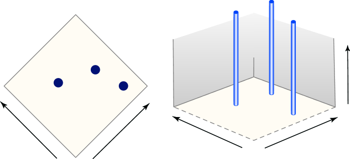
Figure 2. Left panel: singular support of ${\mathcal{P}}$. Right panel: wavefront set of ${\mathcal{P}}$ in phase space.

For the distribution ${\mathcal{C}}$, we obtain

$$\mbox{sing supp}({\mathcal{C}})=image(\tau)\qquad\mbox{and}\qquad WF({\mathcal{C}})=\{(\tau(t),\theta(t)):t\in[0,L(\tau)]\},$$

where $\tau(t)$ is a unit-speed parametrization of ${\mathcal{C}}$ and $\theta(t)$ is the normal direction to ${\mathcal{C}}$ at $\tau(t)$ regarded in ${\bf P}^{1}$. Here, the anisotropy and – in comparison with Figure 2 – the morphological difference to ${\mathcal{P}}$ becomes evident. An illustration of $\mbox{sing supp}({\mathcal{C}})$ and of $WF({\mathcal{C}})$ is presented in Figure 3.

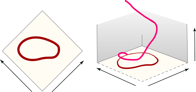
Figure 3. Left panel: singular support of ${\mathcal{C}}$. Right panel: wavefront set of ${\mathcal{C}}$ in phase space.

2.2. Wavelets and Curvelets in Phase Space

Although being smooth functions, in a certain sense, wavelets and curvelets can be regarded as leaving an approximate footprint in phase space. To make this statement rigorous, we first observe the approximate footprint in spatial domain left by wavelet and curvelets as detailed in the following two lemmata taken from [18]. As expected, these observations show the isotropic nature of wavelets in contrast to the anisotropic nature of curvelets.

Lemma 2.1 ([18]).

For each $N=1,2,\dots$ there is a constant $c_{N}$ so that

$$|\psi_{a,b}(x)|\leq c_{N}\cdot a^{-1}\cdot\langle|x-b|/a\rangle^{-N},\qquad\forall a\in{\bf R}^{+}\;\forall b,x\in{\bf R}^{2}.$$

Lemma 2.2 ([18]).

For each $N=1,2,\dots$ there is a constant $c_{N}$ so that

$$|\gamma_{a,b,\theta}(x)|\leq c_{N}\cdot a^{-3/4}\cdot\langle|x-b|_{a,\theta}\rangle^{-N},\qquad\forall a\in{\bf R}^{+}\;\forall\theta\in[0,\pi)\;\forall b,x\in{\bf R}^{2}.$$

Since it is known from [5] that the continuous curvelet transform precisely resolves the wavefront set of distributions, we might consider the image of wavelets and curvelets under the continuous curvelet transform for ‘sufficiently small’ scale as a footprint of these in phase space. An illustration is given in Figure 4, and for a detailed description we refer the interested reader to [18].

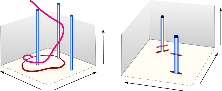
Figure 4. Left panel: wavefront set of the observed data $f={\mathcal{P}}+{\mathcal{C}}$. Right panel: phase space footprint of radial wavelets and curvelets.

Visually, wavelets are perfectly adapted to strongly react to ${\mathcal{P}}$ in a similar way as curvelets will strongly react to ${\mathcal{C}}$. This will be now made precise and will lead to the chosen thresholds for separation.

2.3. Road Map to the ‘Correct’ Thresholds

To slowly approach a rigorous phrasing of the aforementioned strong reaction, we first consider the reaction of both wavelets to ${\mathcal{P}}$ and ${\mathcal{C}}$. A simplified form of Lemma 3.2 states that,

$$|\langle\psi_{a_{j},x_{i}},{\mathcal{P}}_{j}\rangle|=O(2^{j/2})\qquad j\to\infty,$$ (2.1)

with fast decay for other locations than $x_{i}$, and Lemma 3.3 shows that, for each $j$ and $b$,

$$|\langle\psi_{a_{j},b},{\mathcal{C}}_{j}\rangle|=O(1).$$ (2.2)

Secondly, turning our attention to curvelets and their reaction to ${\mathcal{P}}$ and ${\mathcal{C}}$, we observe that, by a simplified form of Lemma 4.4, for each $\theta$,

$$|\langle\gamma_{a_{j},x_{i},\theta},{\mathcal{P}}_{j}\rangle|=O(2^{j/2})\qquad j\to\infty,$$ (2.3)

and, for $b$ positioned on the curve $\tau$ and $\theta$ pointing in the direction perpendicular to the tangent to the curve in $b$,

$$|\langle\gamma_{a_{j},b,\theta},{\mathcal{C}}_{j}\rangle|=O(2^{j/4})\qquad j\to\infty.$$ (2.4)

Examining closely (2.1) and (2.2), it becomes immediately evident that the correct first threshold – which should capture ${\mathcal{P}}_{j}$ by thresholding wavelet coefficients of $f_{j}$ – need to be chosen ‘slightly higher’ than a constant asymptotically, wherefore we choose it equal to $2^{{\varepsilon}j}$ for small ${\varepsilon}$.

The second threshold seem to be a somehow more serious problem, since (2.3) and (2.4) show that curvelets react stronger to a point singularity than a curvilinear singularity. However, we wish the reader to keep in mind that ideally all energy from ${\mathcal{P}}_{j}$ is already captured during the first thresholding procedure. Hence, it should presumably be ‘safe’ to choose the second threshold – which shall capture ${\mathcal{C}}_{j}$ by thresholding curvelet coefficients of the residual ${\mathcal{R}}_{j}$ – with asymptotic behavior $o(2^{j/4})$. To avoid unnecessary risks, we choose it only slightly below $2^{j/4}$, more precisely, equal to $2^{j(1/4-{\varepsilon})}$.

2.4. What Type of Separation Result is Preferable?

Applying now One-Step (cf. Figure 1) yields significant coefficient sets ${\mathcal{T}}_{1,j}$ and ${\mathcal{T}}_{2,j}$ and approximations to ${\mathcal{P}}_{j}$ and ${\mathcal{C}}_{j}$: $W_{j}$ and $C_{j}$. In Sections 1.3 and 1.4, we presented three theorems on the ‘quality’ of this separation, which we would now like to discuss and compare.

Theorem 1.1 studies the relative separation error and proves that asymptotically this error can be made arbitrarily small for sufficiently fine scale. This is in a sense the most natural question to ask, and the theorem provides the answer one would hope for.

However, from a microlocal analysis viewpoint, the most satisfying separation to derive would be the perfect separation of the wavefront sets of ${\mathcal{P}}$ and ${\mathcal{C}}$, i.e., to separate the LHS of Figure 4 into the RHS of Figures 2 and 3. This would be considerably ‘stronger’ than Theorem 1.1 in the following sense: Once the wavefront sets are extracted, we have complete information about the underlying singularities, in contrast to the merely asymptotic knowledge provided by Theorem 1.1.

Knowledge about $WF({\mathcal{P}})$ and $WF({\mathcal{C}})$ could be either coming from ${\mathcal{T}}_{1,j}$ and ${\mathcal{T}}_{2,j}$ or from $W_{j}$ and $C_{j}$. The sets of significant coefficients generated by thresholding do not provide an immediate means for separating the wavefront sets, since they live on the analysis side (as opposed to the synthesis side). Astonishingly, they are still able to precisely locate the wavefront sets $WF({\mathcal{P}})$ and $WF({\mathcal{C}})$, more precisely, they ‘converge’ to the wavefront sets in phase space measured in the phase space norm $d_{PS}$ as $j\to\infty$, which is the statement of Theorem 1.2. This shows that the points in ${\mathcal{T}}_{1,j}$ and ${\mathcal{T}}_{2,j}$ are located in tubes around $WF({\mathcal{P}})$ and $WF({\mathcal{C}})$, respectively, which become more concentrated around these wavefront sets as the scale becomes finer. The corresponding objects on the synthesis side, i.e., $W_{j}$ and $C_{j}$, now allow separation of $WF({\mathcal{P}})$ and $WF({\mathcal{C}})$, in the sense that the wavefront sets of the reconstructed distributions $\sum_{j}F_{j}\star W_{j}$ and $\sum_{j}F_{j}\star C_{j}$ precisely coincide with $WF({\mathcal{P}})$ and $WF({\mathcal{C}})$. This is the content of Theorem 1.3.

3. Geometry of the Thresholded Wavelet Coefficients

Following the ordering of the thresholding, we first focus on the set of significant radial wavelet coefficients ${\mathcal{T}}_{1,j}$ generated by Step 1) of One-Step-Thresholding (see Figure 1), in particular, on its phase space footprint, defined in (1.3) as

$${\mathcal{T}}_{1,j}^{PS}=\{b\in{\bf R}^{2}:|\langle f_{j},\psi_{a_{j},b}\rangle|\geq a_{j}^{-{\varepsilon}}\}\times{\bf P}^{1}.$$

Our objective will be to derive a tube around ${\mathcal{T}}_{1,j}^{PS}$ in phase space with controllable ‘size’. This tube should therefore be a neighborhood of $WF({\mathcal{P}})$, and hence be isotropic.

For our analysis, we first notice that WLOG we can assume that

$${\mathcal{P}}=|x|^{-3/2}.$$ (3.1)

From here, the result for the original ${\mathcal{P}}$ as defined in (1.1) can be concluded because of the following reasons: Firstly, all results are translation invariant, hence instead of the origin the results follow immediately for a different point in spatial domain; and secondly, the change from one point to finitely many points just introduces a constant independent on $j$.

3.1. Estimates for Wavelet Coefficients

We start by analyzing the interaction of wavelet atoms. The technical proof of the following result is provided in Section 8.1

Lemma 3.1.

For each $N=1,2,\dots$, there is a constant $c_{N}$ so that

$$|\langle\psi_{a,b},\psi_{a_{0},b_{0}}\rangle|\leq c_{N}\cdot 1_{\{|\log_{2}(a/a_{0})|<3\}}\cdot\langle|b-b_{0}|/a\rangle^{-N}.$$

Next, we recall a result derived in [18] for radial wavelet coefficients of our point singularity (3.1).

Lemma 3.2 ([18]).

For each $N=1,2,\dots$, there is a constant $c_{N}$ so that

$$|\langle\psi_{a_{j},b},{\mathcal{P}}_{j}\rangle|\leq c_{N}\cdot a_{j}^{-1/2}\cdot\langle|b/a_{j}|\rangle^{-N},\qquad\forall j\in{\bf Z}\;\forall b\in{\bf R}^{2}.$$

In the sequel, we will further require an estimate of the wavelet coefficients of the curvilinear singularity ${\mathcal{C}}_{j}$. Notice that the following estimate does only provide a very coarse upper bound. In order to derive a more detailed estimate, the curve would need to be much more carefully analyzed as it will be done in Section 4. However, the estimate as stated below is all we will require.

Lemma 3.3.

There exists a constant $c$ so that

$$|\langle\psi_{a_{j},b},{\mathcal{C}}\rangle|\leq c,\qquad\forall j\in{\bf Z}\;\forall b\in{\bf R}^{2}.$$

Proof. By Lemma 2.1 and the definition of the distribution ${\mathcal{C}}$,

$$|\langle\psi_{a_{j},b},{\mathcal{C}}\rangle|\leq\int_{0}^{1}|\psi_{a_{j},b}(\tau(t))|\,dt\leq c_{N}\cdot a^{-1}\cdot\int_{0}^{1}\langle|\tau(t)-b|/a\rangle^{-N}dt.$$ (3.2)

WLOG we assume that $b\in\tau([0,1])$ with $\tau(0)=b$, say, and we can also assume that $b=(b_{1},0)$. Choosing a ball $B_{r}(b)$ around $b$ with $r$ chosen arbitrarily small (yet, independent of $j$), there exists some $0<\delta<1/2$ such that

$$\tau([0,1])\cap B_{r}(b)=\tau([1-\delta,1]\cup[0,\delta]).$$

This information is now used to split the last integral in (3.2) according to

$$\int_{0}^{1}\langle|\tau(t)-b|/a\rangle^{-N}dt=\int_{[1-\delta,1]\cup[0,\delta]}\langle|\tau(t)-b|/a\rangle^{-N}dt+\int_{[\delta,1-\delta]}\langle|\tau(t)-b|/a\rangle^{-N}dt=:I_{1}+I_{2}.$$ (3.3)

For estimating $I_{1}$, we first observe that it is sufficient to consider $\int_{[0,\delta]}$ due to symmetry reasons. For $r$ small enough, the curve inside $B_{r}(b)$ can be arbitrarily well approximated by its osculating circle with its center denoted by $z=(z_{1},0)$. Combining these considerations as well as exploiting the approximation by a Taylor series for cosine,

$$\int_{[0,\delta]}\langle|\tau(t)-b|/a\rangle^{-N}dt \leq c\cdot\int_{[0,\delta]}\langle|(b_{1}-z_{1})(\cos(t),\sin(t))+z-b|/a\rangle^{-N}dt$$

$$= c\cdot\int_{[0,\delta]}\langle|b_{1}-z_{1}|\sqrt{2(1-\cos(t))}/a\rangle^{-N}dt$$

$$\leq c^{\prime}\cdot\int_{[0,\delta]}\langle|b_{1}-z_{1}|\cdot t/a\rangle^{-N}dt$$

$$= c^{\prime}\cdot a/|b_{1}-z_{1}|\int_{[0,|b_{1}-z_{1}|\delta/a]}\langle t\rangle^{-N}dt$$

$$\leq c^{\prime\prime}\cdot a/|b_{1}-z_{1}|.$$ (3.4)

Using the definition of $r$, the integral $I_{2}$ can be easily estimated as

$$\int_{[\delta,1-\delta]}\langle|\tau(t)-b|/a\rangle^{-N}dt\leq\int_{[\delta,1-\delta]}\langle r/a\rangle^{-N}dt\leq(r/a)^{-N}.$$ (3.5)

Summarizing, by (3.2)–(3.5), there exists some constant $c$ (independent on $a$ and $b$) such that

$$|\langle\psi_{a_{j},b},{\mathcal{C}}\rangle|\leq c_{N}\cdot a^{-1}\cdot(a/|b_{1}-z_{1}|+(r/a)^{-N})\leq c.$$

The lemma is proved. ∎

3.2. Geometry of ${\mathcal{T}}_{1,j}^{PS}$

We now first analyze the set ${\mathcal{T}}_{1,j}^{PS}$ by the following two lemmata.

Lemma 3.4.

Let $(b,\theta)\in({\mathcal{T}}_{1,j}^{PS})^{c}$, and let $j$ be sufficiently large. Then, for each $N=1,2,\dots$, there is a constant $c_{N}$ so that

$$|b/a_{j}|>c_{N}\cdot 2^{j\frac{1-2{\varepsilon}}{2N}}.$$

Proof. Let $b\in{\bf R}^{2}$ be such that

$$|\langle\psi_{a_{j},b},{\mathcal{P}}_{j}\rangle+\langle\psi_{a_{j},b},{\mathcal{C}}_{j}\rangle|<2^{j{\varepsilon}}.$$

Since by Lemma 3.3, $|\langle\psi_{a_{j},b},{\mathcal{C}}\rangle|$, and hence $|\langle\psi_{a_{j},b},{\mathcal{C}}_{j}\rangle|$, is bounded by a constant $c$, say, we have

$$|\langle\psi_{a_{j},b},{\mathcal{P}}_{j}\rangle|<2^{j{\varepsilon}}+c.$$

Next we use the estimate in Lemma 3.2 as a model to conclude that

$$\langle|b/a_{j}|\rangle^{-N}<c_{N}\cdot 2^{-j/2}(2^{j{\varepsilon}}+c).$$

Thus, since for sufficiently large $j$, we have $2^{j{\varepsilon}}>c$,

$$|b/a_{j}|>\left((c_{N}\cdot 2^{-j/2}(2^{j{\varepsilon}}+c))^{-2/N}-1\right)^{1/2}>\left(c_{N}\cdot 2^{j\frac{1-2{\varepsilon}}{N}}-1\right)^{1/2}.$$

Letting $j$ be large enough so that $(c_{N}/2)\cdot 2^{j\frac{1-2{\varepsilon}}{N}}>1$ proves the lemma. ∎

Lemma 3.5.

Let $(b,\theta)\in{\mathcal{T}}_{1,j}^{PS}$. Then, for each $N=1,2,\dots$, there is a constant $c_{N}$ so that

$$|b/a_{j}|\leq c_{N}\cdot 2^{j\frac{1-2{\varepsilon}}{2N}}.$$

Proof. Let $b\in{\bf R}^{2}$ be such that

$$|\langle\psi_{a_{j},b},{\mathcal{P}}_{j}\rangle+\langle\psi_{a_{j},b},{\mathcal{C}}_{j}\rangle|\geq 2^{j{\varepsilon}}.$$

Since by Lemma 3.3, $|\langle\psi_{a_{j},b},{\mathcal{C}}\rangle|$, and hence $|\langle\psi_{a_{j},b},{\mathcal{C}}_{j}\rangle|$, is bounded by a constant $c$, say, we have

$$|\langle\psi_{a_{j},b},{\mathcal{P}}_{j}\rangle|\geq 2^{j{\varepsilon}}-c.$$

Next we use the estimate in Lemma 3.2 as a model to conclude that

$$\langle|b/a_{j}|\rangle^{-N}\geq c_{N}\cdot 2^{-j/2}(2^{j{\varepsilon}}-c).$$

Thus, since for sufficiently large $j$, we have $2^{j{\varepsilon}-1}>c$,

$$|b/a_{j}|\leq\left((c_{N}\cdot 2^{-j/2}(2^{j{\varepsilon}}-c))^{-2/N}-1\right)^{1/2}\leq\left(c_{N}\cdot 2^{j\frac{1-2{\varepsilon}}{N}}\right)^{1/2}.$$

The lemma is proved. ∎

We certainly hope (and expect) that the threshold is set in such a way that the wavefront set of ${\mathcal{P}}$ is contained in ${\mathcal{T}}_{1,j}^{PS}$. This is obviously the first requirement for being able to separate both wavefront sets $WF({\mathcal{P}})$ and $WF({\mathcal{C}})$ through Single-Pass Alternating Thresholding (compare Theorem 1.3). The next result shows that this is indeed the case.

Lemma 3.6.

For $j$ sufficiently large,

$$|\langle{\mathcal{P}}_{j},\psi_{a_{j},0}\rangle|\geq c\cdot 2^{j/2}.$$

Hence, in particular,

$$WF({\mathcal{P}})\subseteq{\mathcal{T}}_{1,j}^{PS}.$$

Proof. By Parseval,

$$|\langle{\mathcal{P}}_{j},\psi_{a_{j},0}\rangle|=2\pi|\langle\hat{{\mathcal{P}}}_{j},\hat{\psi}_{a_{j},0}\rangle|=2\pi\cdot 2^{j/2}\int W^{2}(|\xi|)|\xi|^{-1/2}d\xi.$$

Hence, we can conclude that, for $j$ sufficiently large,

$$|\langle{\mathcal{P}}_{j},\psi_{a_{j},0}\rangle|\geq c\cdot 2^{j/2}.$$

This proves the first claim.

For the ‘in particular’-part, recall that $WF({\mathcal{P}})=\{0\}\times\mathbf{P}^{1}$. By Lemma 3.3 and the previous consideration, for sufficiently large $j$,

$$|\langle f_{j},\psi_{a_{j},0}\rangle|\geq|\langle{\mathcal{P}}_{j},\psi_{a_{j},0}\rangle|-|\langle{\mathcal{C}}_{j},\psi_{a_{j},0}\rangle|\geq|\langle{\mathcal{P}}_{j},\psi_{a_{j},0}\rangle|-c\geq 2^{{\varepsilon}j}.$$

The lemma is proved. ∎

4. Geometry of the Thresholded Curvelet Coefficients

This section now aims to derive a fundamental geometric understanding of the cluster of curvelet coefficients ${\mathcal{T}}_{2,j}$ generated by Step 3) of One-Step-Thresholding of the residual generated in Step 2) (see Figure 1). The phase space geometry will play an essential role in setting up the analysis correctly, hence it will be beneficial to study the projection of ${\mathcal{T}}_{2,j}$ onto phase space, defined in (1.4), as

$${\mathcal{T}}_{2,j}^{PS}=\{(b,\theta)\in{\bf R}^{2}\times[0,\pi):|\langle{\mathcal{R}}_{j},\gamma_{a_{j},b,\theta}\rangle|\geq a_{j}^{{\varepsilon}-1/4}\}.$$

Morally, the points in phase space associated with significant curvelet coefficients, given by ${\mathcal{T}}_{2,j}^{PS}$, are contained in a tube around $WF(w{\mathcal{L}})$ in phase space. The main objective will now be to explicitly define such a tube around the phase space footprint of this cluster, where we have more control on. This will become crucial for handling the thresholded curvelet coefficients in the proofs of Theorems 1.1–1.3.

4.1. Bending the Curve

We first face the problem of how to deal with the curvilinear singularity. In [18], this problem was tackled by carefully and smoothly breaking the curve into pieces, bending each piece, and then combining pieces in the end. This technique shall also be applied here. For the convenience of the reader, we review the main ideas of this particular approach.

First, a quantitative ‘tubular neighborhood theorem’ is being developed to allow local bending of the curve. Due to regularity of the curve, there exists some $\rho$ small compared to the curvature of $\tau$, so that

$$\int_{(i-1)\rho}^{(i+1)\rho}|\tau^{{}^{\prime\prime}}(t)|dt\leq{\varepsilon},\qquad i=0,...,\tfrac{{\rm length}(\tau)}{\rho}=:m.$$

Now consider the following local coordinate system in the vicinity of $\tau$. Let $t_{i}=i\rho$, for $i=0,\dots,m$ with $\tau(t_{0})=\tau(t_{m})$, since $\tau$ is closed. Then we have the following

Lemma 4.1 ([18]).

(Tubular Neighborhood Theorem) For sufficiently small ${\varepsilon}>0$, there is some ${\varepsilon}^{\prime}>0$ so that, for $X_{{\varepsilon}^{\prime}}=[-{\varepsilon}^{\prime},{\varepsilon}^{\prime}]\times[-\rho,\rho]$, we have:

• for each $i=0,\dots,m$, there exists a tube $Y_{{\varepsilon}^{\prime}}^{i}$ around $\tau$ and an associated diffeomorphism $\phi^{i}:Y_{{\varepsilon}^{\prime}}^{i}\mapsto X_{{\varepsilon}^{\prime}}$,

• the mapping $\phi^{i}$ extends to a diffeomorphism from ${\bf R}^{2}$ to ${\bf R}^{2}$ which reduces to the identity outside a compact set.

Thus, the set $Y_{{\varepsilon}^{\prime}}=\cup_{i}Y_{{\varepsilon}^{\prime}}^{i}$ is a tubular neighborhood of $image(\tau)$ on which we have nice local coordinate systems, see Figure 5. This will allow us to locally bend the curve $\tau$. From now on, $\phi^{i}$ always denotes the extended diffeomorphism from ${\bf R}^{2}$ to ${\bf R}^{2}$.

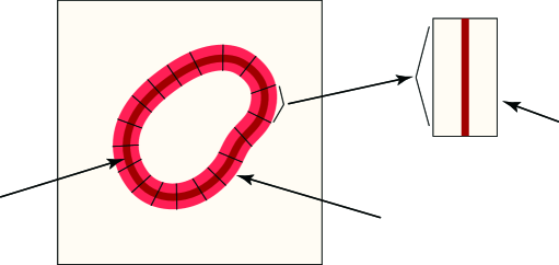
Figure 5. The tubular neighborhood $Y_{{\varepsilon}^{\prime}}=\cup_{i}Y_{{\varepsilon}^{\prime}}^{i}$ of $image(\tau)$ and the mapping $\phi^{i}:Y_{{\varepsilon}^{\prime}}^{i}\mapsto X_{{\varepsilon}^{\prime}}$.

Next, choose a $C^{\infty}$ function $w_{2}:{\bf R}\mapsto[0,1]$ supported in $[-1,1]$ satisfying

$$|\hat{w}_{2}(\omega)|\leq c\cdot e^{-|\omega|},\quad\omega\in{\bf R}$$ (4.1)

and

$$w_{2}(\tfrac{t}{\rho})+w_{2}(\tfrac{t-1}{\rho})=1\>(-\tfrac{1}{2}\leq t\leq 0)\quad\mbox{and}\quad w_{2}(\tfrac{t}{\rho})+w_{2}(\tfrac{t+1}{\rho})=1\>(0\leq t\leq\tfrac{1}{2}).$$

Define a smooth partition of unity of $[0,1]$ using $w_{2}$ by

$$w_{2,i}(t/\rho)=w_{2}((t-t_{i})/\rho),\qquad 1\leq i\leq m,$$

and accordingly the distributions

$${\mathcal{C}}^{i}=\int_{t_{i-1}}^{t_{i+1}}w_{2,i}(t/\rho)\delta_{\tau(t)}dt;$$

the partition of unity property giving $\sum_{i}{\mathcal{C}}^{i}={\mathcal{C}}$.

Now consider the action of $\phi^{i}$ on the distribution $f$

$$(\phi^{i})^{\star}f=f\circ\phi^{i}.$$

This action induces a linear transformation on the space of curvelet coefficients. With $\alpha(f)$ the curvelet coefficients of $f$ and $\beta(f)$ the curvelet coefficients of $(\phi^{i})^{\star}f$, we obtain a linear operator

$$M_{\phi^{i}}(\alpha(f))=\beta(f).$$

It is by now well-known that diffeomorphisms preserve sparsity of frame coefficients when the frame is based on parabolic scaling (as with curvelets and shearlets), e.g., by [35] (see also [6, Theorem 6.1, page 219]), for any $0<p\leq 1$,

$$\|M_{\phi}\|_{Op,p}:=\max\left\{\sup_{\eta}\|(\langle\gamma_{\eta},\phi^{\star}\gamma_{\eta^{\prime}}\rangle)_{\eta}\|_{p},\sup_{\eta^{\prime}}\|(\langle\gamma_{\eta},\phi^{\star}\gamma_{\eta^{\prime}}\rangle)_{\eta^{\prime}}\|_{p}\right\}<\infty.$$

After having carefully bended the curve pieces, we can also reserve the process and glue them together. Choosing, e.g., $\beta_{j}=(\langle\gamma_{\eta},{\mathcal{C}}_{j}\rangle)_{\eta}$, from the decomposition ${\mathcal{C}}_{j}=\sum_{i=1}^{m}{\mathcal{C}}^{i}_{j}$ we have

$$\beta_{j}=\sum_{i=1}^{m}M_{\phi^{i}}\alpha_{j}.$$

This decomposition allows us to relate sparsity of coefficients of the linear singularity to those of the curvilinear singularity:

$$\|\beta_{j}\|_{p} \leq m^{1/p}\cdot\left(\max_{i}\|M_{\phi^{i}}\|_{Op,p}\right)\cdot\|\alpha_{j}\|_{p}.$$ (4.2)

Finally, we define the very special distribution $w{\mathcal{L}}$ we will consider, supported on a line segment $\{0\}\times[-\rho,\rho]$ by

$$w{\mathcal{L}}=w_{2}(x_{2}/\rho)\cdot\delta_{0}(x_{1}).$$

Then we can write

$$\widehat{w{\mathcal{L}}}=\hat{w}\star\hat{{\mathcal{L}}},$$

where

$$\hat{w}=\hat{w}_{2}(\rho\xi_{2})\cdot\rho\cdot\delta_{0}(\xi_{1})\quad\mbox{and}\quad\hat{{\mathcal{L}}}=\delta_{0}(\xi_{2}).$$

Thus the action of $w{\mathcal{L}}$ on a continuous function $f$ is given by

$$2\pi\langle w{\mathcal{L}},f\rangle=\langle{\mathcal{L}},\hat{w}\star\hat{f}\rangle=\int(\hat{w}\star\hat{f})(\xi_{1},0)d\xi_{1}.$$

Conceptually, $w{\mathcal{L}}$ is a straight curve fragment, which the approach taken in [18] reduced the analysis of ${\mathcal{C}}$ to.

Concluding this approach enables us to consider curvelet coefficients of a linear singularity instead of a curvilinear singularity with a linear operator mapping one coefficient set onto the other.

4.2. Estimates for Curvelet Coefficients

We start by estimating the interaction of curvelet atoms and the interaction of a curvelet atom with a wavelet atom. These results are proved in [18].

Lemma 4.2 ([18]).

For each $N=1,2,\dots$, there is a constant $c_{N}$ so that

$$|\langle\gamma_{a,b,\theta},\gamma_{a_{0},b_{0},\theta_{0}}\rangle|\leq c_{N}\cdot 1_{\{|\log_{2}(a/a_{0})|<3\}}\cdot 1_{\{|\theta-\theta_{0}|<10\sqrt{a_{0}}\}}\cdot\langle|b-b_{0}|_{a_{0},\theta_{0}}\rangle^{-N}.$$

Lemma 4.3 ([18]).

For each $N=1,2,\dots$, there is a constant $c_{N}$ so that

$$|\langle\gamma_{a,b,\theta},\psi_{a_{0},b_{0}}\rangle|\leq c_{N}\cdot a^{1/4}\cdot 1_{\{|\log_{2}(a/a_{0})|<3\}}\cdot\langle|b-b_{0}|_{a,\theta}\rangle^{-N}.$$

We now first analyze curvelet coefficients of the point singularity ${\mathcal{P}}$. The technical proof will be given in Subsection 8.2.

Lemma 4.4.

For each $N=1,2,\dots$, there is a constant $c_{N}$ so that

$$|\langle{\mathcal{P}}_{j},\gamma_{a_{j},b,\theta}\rangle|\leq c_{N}\cdot a_{j}^{-1/2}\cdot\langle|D_{1/a_{j}}b|\rangle^{-N},\qquad\forall j\in{\bf Z}\;\forall b,\theta.$$

Next we state two lemmata from [18], which provide estimates for the curvelet coefficients of our linear singularity by first considering curvelets, which are almost aligned with the singularity, and secondly considering the remaining ones.

Lemma 4.5 ([18]).

Suppose that $\theta\in[0,\sqrt{a}]$, and set

$$\tau:=\cos\theta\sin\theta(a^{-1}-a^{-2}),\quad d_{1}^{2}=b_{1}^{2}(\sigma_{2}^{2}-\sigma_{1}^{-2}\tau),$$

and

$$d_{2}^{2}=\left\{\begin{array}[]{ccl}\min\{((\rho-b_{2})\sigma_{1}+\sigma_{1}^{-1}b_{1}\tau)^{2},((-\rho-b_{2})\sigma_{1}+\sigma_{1}^{-1}b_{1}\tau)^{2}\}&:&b_{2}-\sigma_{1}^{-2}b_{1}\tau\not\in[-\rho,\rho],\\ 0&:&b_{2}-\sigma_{1}^{-2}b_{1}\tau\in[-\rho,\rho],\end{array}\right.$$

where

$$\sigma_{1}=(a^{-2}\sin^{2}\theta+a^{-1}\cos^{2}\theta)^{1/2}\quad\mbox{and}\quad\sigma_{2}=(a^{-1}\sin^{2}\theta+a^{-2}\cos^{2}\theta)^{1/2}.$$

Then, for $N=1,2,\ldots$,

$$|\langle w{\mathcal{L}},\gamma_{a,b,\theta}\rangle|\leq c_{N}\cdot a^{-3/4}\cdot\sigma_{1}^{-1}\cdot\langle d_{1}\rangle^{-1}\cdot\langle|(d_{1},\sigma_{1}d_{2})|\rangle^{2-N}.$$

In particular, if $\theta=0$,

$$|\langle w{\mathcal{L}},\gamma_{a,b,\theta}\rangle|\leq c_{N}\cdot a^{-1/4}\cdot\langle|b_{1}/a|\rangle^{-1}\cdot\langle a^{-1}[|b_{1}|^{2}+\min\{(b_{2}-\rho)^{2},(b_{2}+\rho)^{2}\}]^{1/2}\rangle^{2-N},$$

and, if $\theta=0$ and $b_{2}\in[-\rho,\rho]$,

$$|\langle w{\mathcal{L}},\gamma_{a,b,\theta}\rangle|\leq c_{N}\cdot a^{-1/4}\cdot\langle|b_{1}/a|\rangle^{1-N}.$$

Lemma 4.6 ([18]).

Suppose that $\theta\in(\sqrt{a},\pi)$. Then, for $N=1,2,\ldots$,

$$|\langle w{\mathcal{L}},\gamma_{a,b,\theta}\rangle| \leq c_{L,M}\cdot a^{-1/4}\cdot|\cos\theta|\cdot e^{-\rho\frac{|\sin\theta|}{2a}}\cdot\langle|b_{1}|\rangle^{-L}\cdot(a^{1/2}|\sin\theta|+a|\cos\theta|)^{L}$$

$$\cdot\langle|b_{2}|\rangle^{-M}\cdot(\rho+a^{1/2}|\cos\theta|+a|\sin\theta|)^{M}.$$

4.3. Relation of ${\mathcal{T}}_{2,j}^{PS}$ to Significant Coefficients from $\ell_{1}$ Minimization

Comparing the set of significant coefficients ${\mathcal{T}}_{2,j}$ we derive from thresholding with the set of significant coefficients associated with $\ell_{1}$ minimization studied in [18] will be quite beneficial, since it will later on allow us to exploit some of the results from this paper.

To start, we briefly review the definitions and choices made for the significant curvelet coefficients associated with $\ell_{1}$ minimization. Recalling the definition of the straight curve fragment $w{\mathcal{L}}$ from Section 4.1, we first define a neighborhood of $WF(w{\mathcal{L}})$ by

$${\mathcal{N}}^{PS}(a,c,{\varepsilon}^{\prime})=\{b\in{\bf R}^{2}:d_{2}(b,\{0\}\times[-2\rho,2\rho])\leq c\cdot D_{2}(a,{\varepsilon}^{\prime})\}\times[0,\sqrt{a}],$$ (4.3)

where $c>0$ is some constant and

$$D_{2}(a,{\varepsilon}^{\prime})=a^{(1-{\varepsilon}^{\prime})}\qquad\mbox{for some }{\varepsilon}^{\prime}>0.$$

Then the set of significant curvelet coefficients for $w{\mathcal{L}}$ was in [18] chosen as

$$\tilde{{\mathcal{S}}}_{j}(c,{\varepsilon}^{\prime})=\{(j,k,\ell)\in\bigcup_{j^{\prime}=j-1}^{j+1}\Delta_{j^{\prime}}:(b_{j,k,\ell},\theta_{j,\ell})\in{\mathcal{N}}^{PS}(a_{j},c,{\varepsilon}^{\prime})\}.$$

Let us now first consider the set $\tilde{{\mathcal{T}}}_{2,j}$ defined by

$$\tilde{{\mathcal{T}}}_{2,j}=\{\eta:|\langle w{\mathcal{L}}_{j},\gamma_{\eta}\rangle|\geq 2^{j(1/4-{\varepsilon})}\},$$

which is related to $\tilde{{\mathcal{S}}}_{j}$ in the following way:

Proposition 4.1.

There exist $c_{1},c_{2}>0$ and ${\varepsilon}^{\prime}_{1},{\varepsilon}^{\prime}_{2}\in(0,{\varepsilon})$ such that

$$\tilde{{\mathcal{S}}}_{j}(c_{1},{\varepsilon}^{\prime}_{1})\subseteq\tilde{{\mathcal{T}}}_{2,j}\subseteq\tilde{{\mathcal{S}}}_{j}(c_{2},{\varepsilon}^{\prime}_{2}).$$

Proof. We first prove $\tilde{{\mathcal{T}}}_{2,j}\subseteq\tilde{{\mathcal{S}}}_{j}(c_{2},{\varepsilon}^{\prime}_{2})$. Using the estimate in Lemma 4.5 as a model, we obtain the following: For all $(b_{j,k,\ell},\theta_{j,\ell})$ with $(j,k,\ell)\in\tilde{{\mathcal{T}}}_{2,j}$ and $N=1,2,\ldots$, we have

$$\sigma_{1}^{\frac{1}{N-2}}\cdot\langle d_{1}\rangle^{\frac{1}{N-2}}\cdot\langle|(d_{1},\sigma_{1}d_{2})|\rangle\leq c_{N}\cdot 2^{j\frac{1/2+{\varepsilon}}{N-2}}.$$

Now Lemma 4.6 implies that WLOG we only need to consider the case $\theta\in[0,\sqrt{a}]$ due to the rapidly decaying exponential factor. To obtain an estimate for $b$, also WLOG we can assume that $\theta=0$, which implies

$$a^{-\frac{1}{2(N-2)}}\cdot\langle|b_{1}/a|\rangle^{\frac{1}{N-2}}\cdot\langle a^{-1}[|b_{1}|^{2}+\min_{\pm}(b_{2}\pm\rho)^{2}]^{1/2}\rangle\leq c_{N}\cdot 2^{j\frac{1/2+{\varepsilon}}{N-2}},$$

which is equivalent to

$$\langle|b_{1}/a|\rangle^{\frac{1}{N-2}}\cdot\langle a^{-1}[|b_{1}|^{2}+\min_{\pm}(b_{2}\pm\rho)^{2}]^{1/2}\rangle\leq c_{N}\cdot 2^{j\frac{{\varepsilon}}{N-2}}.$$ (4.4)

Since both factors are larger than $1$, we can split this inequality into

$$\langle|b_{1}/a|\rangle^{\frac{1}{N-2}}\leq c_{N}\cdot 2^{j\frac{{\varepsilon}}{N-2}}$$ (4.5)

and

$$\langle a^{-1}[|b_{1}|^{2}+\min_{\pm}(b_{2}\pm\rho)^{2}]^{1/2}\rangle\leq c_{N}\cdot 2^{j\frac{{\varepsilon}}{N-2}}.$$ (4.6)

From (4.5), we conclude that

$$|b_{1}|\leq c_{N}\cdot 2^{-j(1-{\varepsilon})},$$ (4.7)

and from (4.6), we conclude that

$$\min_{\pm}|b_{2}\pm\rho|\leq c_{N}\cdot 2^{-j(1-\frac{{\varepsilon}}{N-2})}.$$ (4.8)

Thus, for $c_{2}$ and ${\varepsilon}^{\prime}_{2}\in(0,{\varepsilon})$ appropriately chosen,

$$\tilde{{\mathcal{T}}}_{2,j}\subseteq\tilde{{\mathcal{S}}}_{j}(c_{2},{\varepsilon}^{\prime}_{2}).$$

The converse inclusion can be derived by substituting (4.7) and (4.8) into (4.4). This proves the lemma. ∎

However, we wish to remind the reader that it is the set of significant curvelet coefficients of the curvilinear singularity we aim to analyze. For this reason, in the approach presented in [18], the aforementioned linear operator was exploited to obtain the set of significant curvelet coefficients of ${\mathcal{C}}$ based on the chosen set $\tilde{{\mathcal{S}}}_{j}(c,{\varepsilon}^{\prime})$ for $w{\mathcal{L}}$. For this, let $M_{F_{j}}=(\langle\gamma_{\eta},F_{j}\star\gamma_{\eta^{\prime}}\rangle)_{\eta,\eta^{\prime}}$ be the filtering matrix associated with the filter $F_{j}$. The ‘correct’ linear operator to consider is defined by the matrix

$$M_{j}^{i}=M_{F_{j}}\cdot M_{(\phi^{i})^{-1}},$$

and the entries of this matrix will be denoted by $M_{j}^{i}(\eta,\eta^{\prime})$. Further, we let $t_{\eta^{\prime},n}$ denote the amplitude of the $n$’th largest element of the $\eta^{\prime}$’th column. Now setting

$${\mathcal{S}}_{j}^{i}(c,{\varepsilon}^{\prime})=\{\eta:\eta^{\prime}\in\tilde{{\mathcal{S}}}_{j}(c,{\varepsilon}^{\prime})\mbox{ and }|M_{j}^{i}(\eta,\eta^{\prime})|>t_{\eta^{\prime},2^{j{\varepsilon}^{\prime}}}\},$$

the overall cluster set of significant curvelet coefficients of ${\mathcal{C}}$ is

$${\mathcal{S}}_{2,j}(c,{\varepsilon}^{\prime})=\bigcup_{i}{\mathcal{S}}_{j}^{i}(c,{\varepsilon}^{\prime}).$$

Highly technical and tedious computations (compare [18, Sec. 7]) – which we decided to not repeat here due to their non-intuitive nature – then imply the following result by using Proposition 4.1.

Proposition 4.2.

There exist $c_{1},c_{2}>0$ and ${\varepsilon}^{\prime}_{1},{\varepsilon}^{\prime}_{2}\in(0,{\varepsilon})$ such that

$${\mathcal{S}}_{2,j}(c_{1},{\varepsilon}^{\prime}_{1})\subseteq\{\eta:|\langle{\mathcal{C}}_{j},\gamma_{\eta}\rangle|\geq 2^{j(1/4-{\varepsilon})}\}\subseteq{\mathcal{S}}_{2,j}(c_{2},{\varepsilon}^{\prime}_{2}).$$

This observation ensures that results from [18] concerning the set of significant curvelet coefficients are transferable to the situation under consideration in this paper; pleasing news which we intend to take advantage of.

4.4. Geometry of ${\mathcal{T}}_{2,j}^{PS}$

Our next goal is to show that instead of considering the set ${\mathcal{T}}_{2,j}$ which depends on the residual ${\mathcal{R}}_{j}$ – typically difficile to handle – we might consider the ‘easier-to-handle’ set

$$\{\eta:|\langle{\mathcal{C}}_{j},\gamma_{\eta}\rangle|\geq 2^{j(1/4-{\varepsilon}^{\prime})}\}$$

with some control on ${\varepsilon}^{\prime}$. This requires a careful analysis of the behavior of the coefficients $\langle{\mathcal{R}}_{j},\gamma_{\eta}\rangle$, which are of the following form:

Lemma 4.7.

We have

$$\langle{\mathcal{R}}_{j},\gamma_{\eta}\rangle=\langle{\mathcal{C}}_{j},\gamma_{\eta}\rangle-\sum_{\lambda\in{\mathcal{T}}_{1,j}}\langle{\mathcal{C}}_{j},\psi_{\lambda}\rangle\langle\psi_{\lambda},\gamma_{\eta}\rangle+\sum_{\lambda\in{\mathcal{T}}_{1,j}^{c}}\langle{\mathcal{P}}_{j},\psi_{\lambda}\rangle\langle\psi_{\lambda},\gamma_{\eta}\rangle.$$

Proof. We compute

$$\langle{\mathcal{R}}_{j},\gamma_{\eta}\rangle=\langle{\mathcal{P}}_{j},\gamma_{\eta}\rangle+\langle{\mathcal{C}}_{j},\gamma_{\eta}\rangle-\langle\sum_{\lambda\in{\mathcal{T}}_{1,j}}\langle{\mathcal{P}}_{j},\psi_{\lambda}\rangle\psi_{\lambda},\gamma_{\eta}\rangle-\sum_{\lambda\in{\mathcal{T}}_{1,j}}\langle{\mathcal{C}}_{j},\psi_{\lambda}\rangle\langle\psi_{\lambda},\gamma_{\eta}\rangle.$$

Using the fact that $(\psi_{\lambda})_{\lambda}$ is a tight frame, we conclude that

$$\langle{\mathcal{P}}_{j},\gamma_{\eta}\rangle-\langle\sum_{\lambda\in{\mathcal{T}}_{1,j}}\langle{\mathcal{P}}_{j},\psi_{\lambda}\rangle\psi_{\lambda},\gamma_{\eta}\rangle=\sum_{\lambda\in{\mathcal{T}}_{1,j}^{c}}\langle{\mathcal{P}}_{j},\psi_{\lambda}\rangle\langle\psi_{\lambda},\gamma_{\eta}\rangle,$$

and the lemma is proved. ∎

The threshold was chosen precisely so that $\langle{\mathcal{R}}_{j},\gamma_{\eta}\rangle\approx\langle{\mathcal{C}}_{j},\gamma_{\eta}\rangle$ for all $\eta$ asymptotically, i.e., that the two residuals in Lemma 4.7 become asymptotically negligible. A quantitative statement of this consideration is

Proposition 4.3.

For any $\delta>0$,

$$\Bigg{|}\sum_{\lambda\in{\mathcal{T}}_{1,j}}\langle{\mathcal{C}}_{j},\psi_{\lambda}\rangle\langle\psi_{\lambda},\gamma_{\eta}\rangle+\sum_{\lambda\in{\mathcal{T}}_{1,j}^{c}}\langle{\mathcal{P}}_{j},\psi_{\lambda}\rangle\langle\psi_{\lambda},\gamma_{\eta}\rangle\Bigg{|}=O(2^{-j(1/4-\delta)}),\qquad j\to\infty.$$

In particular, we have

$$\{\eta:|\langle{\mathcal{C}}_{j},\gamma_{\eta}\rangle|\geq 2^{j(1/4-({\varepsilon}-\delta))}\}\subseteq\{\eta:|\langle{\mathcal{R}}_{j},\gamma_{\eta}\rangle|\geq 2^{j(1/4-{\varepsilon})}\}\subseteq\{\eta:|\langle{\mathcal{C}}_{j},\gamma_{\eta}\rangle|\geq 2^{j(1/4-({\varepsilon}+\delta))}\}.$$

Proof. Let $\delta>0$ be arbitrary. For proving the first claim, we consider both terms on the LHS separately. By Lemmata 3.3 and 4.3,

$$\Bigg{|}\sum_{\lambda\in{\mathcal{T}}_{1,j}}\langle{\mathcal{C}}_{j},\psi_{\lambda}\rangle\langle\psi_{\lambda},\gamma_{\eta}\rangle\Bigg{|}\leq c\cdot\sum_{\lambda\in{\mathcal{T}}_{1,j}}|\langle\psi_{\lambda},\gamma_{\eta}\rangle|\\ \leq c\cdot|{\mathcal{T}}_{1,j}|\cdot 2^{-j/4}.$$

Since Lemma 3.5 implies that

$$|{\mathcal{T}}_{1,j}|\leq c_{N}\cdot 2^{j\frac{1-2{\varepsilon}}{N}},$$

we obtain

$$\Bigg{|}\sum_{\lambda\in{\mathcal{T}}_{1,j}}\langle{\mathcal{C}}_{j},\psi_{\lambda}\rangle\langle\psi_{\lambda},\gamma_{\eta}\rangle\Bigg{|}\leq c_{N}\cdot 2^{j\frac{1-2{\varepsilon}}{N}-j/4}.$$

For $N$ large enough,

$$\Bigg{|}\sum_{\lambda\in{\mathcal{T}}_{1,j}}\langle{\mathcal{C}}_{j},\psi_{\lambda}\rangle\langle\psi_{\lambda},\gamma_{\eta}\rangle\Bigg{|}\leq c\cdot 2^{-j(1/4-\delta)},\qquad j\to\infty.$$ (4.9)

Secondly, by Lemmata 3.2 and 3.4,

$$\sum_{\lambda\in{\mathcal{T}}_{1,j}^{c}}|\langle{\mathcal{P}}_{j},\psi_{\lambda}\rangle|\leq c_{N}\cdot\sum_{|k|>c_{N}\cdot 2^{j\frac{1-2{\varepsilon}}{2N}}}2^{j/2}\cdot\langle|k|\rangle^{-N}.$$ (4.10)

For $N$ large enough, we have

$$\int_{\{x:|x|>c_{N}\cdot 2^{j\frac{1-2{\varepsilon}}{2N}}\}}\langle|x|\rangle^{-N}dx_{2}dx_{2}\leq c_{N}\cdot 2^{j(1-N)\frac{1-2{\varepsilon}}{N}}\leq c_{N}\cdot 2^{-j(1/2-\delta)}.$$ (4.11)

By (4.10) and (4.11), also exploiting Lemma 4.3,

$$\Bigg{|}\sum_{\lambda\in{\mathcal{T}}_{1,j}^{c}}\langle{\mathcal{P}}_{j},\psi_{\lambda}\rangle\langle\psi_{\lambda},\gamma_{\eta}\rangle\Bigg{|}\leq c\cdot 2^{j\delta}\cdot 2^{-j/4}\leq c\cdot 2^{-j(1/4-\delta)},\qquad j\to\infty.$$ (4.12)

Now the first claim follows from (4.9) and (4.12).

The ‘in particular’-part can now be derived as a consequence of the first claim by using Lemma 4.7. ∎

Lemma 3.6 already proved that $WF({\mathcal{P}})\subseteq{\mathcal{T}}_{1,j}^{PS}$. Our last result in this subsection shows that a similar result holds true for the wavefront set of ${\mathcal{C}}$ and the thresholding set ${\mathcal{T}}_{2,j}^{PS}$. These two results will be one main ingredient for proving the separation of wavefront sets through Single-Pass Alternating Thresholding stated in Theorem 1.3.

Lemma 4.8.

For $j$ sufficiently large,

$$|\langle w{\mathcal{L}}_{j},\gamma_{j,(0,k_{2}),0}\rangle|\geq 2^{j(1/4-{\varepsilon})}\qquad\forall\,k_{2}\in 2^{j}[-\rho,\rho].$$

Hence, in particular,

$$WF({\mathcal{C}})\cap\{(b_{j,k,\ell},\theta_{j,\ell}):(j,k,\ell)\in\Delta_{j}\}\subseteq{\mathcal{T}}_{2,j}^{PS}.$$

Proof. By Parseval,

$$|\langle w{\mathcal{L}}_{j},\gamma_{j,(0,k_{2}),0}\rangle| = 2\pi|\langle\hat{w{\mathcal{L}}}_{j},\hat{\gamma}_{j,(0,k_{2}),0}\rangle|$$

$$= 2\pi\cdot 2^{-3j/4}\cdot\int\rho\cdot\hat{w}_{2}(-\rho\xi_{2})W(|\xi|/2^{j})V(2^{j/2}\omega)e^{i(k_{2}/2^{j/2})\xi_{2}}d\xi.$$

Apply the change of variables $\zeta=(\xi_{1}/2^{j},\xi_{2})$ and $d\zeta=2^{j}d\xi$,

$$|\langle w{\mathcal{L}}_{j},\gamma_{j,(0,k_{2}),0}\rangle|=2\pi\rho\cdot 2^{j/4}\cdot\int\hat{w}_{2}(-\rho\zeta_{2})\left[\int W(|\zeta^{(j)}|)V(2^{j/2}\omega(\zeta))d\zeta_{1}\right]e^{i(k_{2}/2^{j/2})\zeta_{2}}d\zeta_{2}.$$ (4.13)

where $\zeta^{(j)}=(\zeta_{1},\zeta_{2}/2^{j})$ and $\omega(\zeta)$ denotes the angular component of the polar coordinates of $\zeta$. As $j\to\infty$, the integration area is asymptotically (as $j\to\infty$) of the form

$$\Xi=([-2,-1/2]\cup[1/2,2])\times[-2^{j/2},2^{j/2}].$$

Letting $L_{\delta}=2^{j(1/2-\delta)}$, the choice of $W$ and $V$ implies that the dependence of

$$[-L_{\delta},L_{\delta}]\ni\zeta_{2}\mapsto\int W(|\zeta^{(j)}|)V(2^{j/2}\omega(\zeta))d\zeta_{1}$$

on $j$ is asymptotically negligible, and that its absolute value is uniformly bounded from below. Thus, by (4.13) and taking the rapid decay condition (4.1) on $\hat{w}_{2}$ into account, for some $c>0$,

$$|\langle w{\mathcal{L}}_{j},\gamma_{j,(0,k_{2}),0}\rangle|\geq c\cdot 2^{j/4}\cdot\int\hat{w}_{2}(-\rho\zeta_{2})e^{i(k_{2}/2^{j/2})\zeta_{2}}d\zeta_{2}.$$ (4.14)

Finally, again by (4.1), we can conclude that there exists some $c^{\prime}>0$ such that

$$\int\hat{w}_{2}(-\rho\zeta_{2})e^{i(k_{2}/2^{j/2})\zeta_{2}}d\zeta_{2}\geq c^{\prime},\quad\forall k_{2}\in 2^{j}[-\rho,\rho].$$ (4.15)

Combining (4.14) and (4.15), for sufficiently large $j$,

$$|\langle w{\mathcal{L}}_{j},\gamma_{j,(0,k_{2}),0}\rangle|\geq 2^{j(1/4-{\varepsilon})},\quad\forall k_{2}\in 2^{j}[-\rho,\rho]$$ (4.16)

which was claimed.

For the ‘in particular’-part, we first observe that due to Proposition 4.3, WLOG we can consider

$$\{\eta:|\langle{\mathcal{C}}_{j},\gamma_{\eta}\rangle|\geq 2^{j(1/4-({\varepsilon}+\delta))}\}$$

for defining ${\mathcal{T}}_{2,j}^{PS}$. We then employ the careful bending of the curve as detailed in Section 4.1, Proposition 4.2, [18, Lem. 7.8], and Proposition 4.1, as well as the fact that $WF(w{\mathcal{L}})=\{(0,b):b\in[-\rho,\rho]\}\times\{0\}$. This consideration allows us to conclude that the claim follows from (4.16). ∎

5. Asymptotic Separation

This section is devoted to the analysis around and to the proof of Theorem 1.1. We first consider an abstract separation setting, which we will subsequently apply to each filtered version of an image composed of pointline and curvelike structures.

5.1. Abstract Separation Estimate for Thresholding

Suppose we have two tight frames $\Phi_{1}=(\phi_{1,i})_{i}$, $\Phi_{2}=(\phi_{2,j})_{j}$ in a Hilbert space ${\mathcal{H}}$, and a signal vector $S\in{\mathcal{H}}$. We assume that all frame vectors are normalized to $c$, say, i.e.,

$$\|\phi_{1,i}\|_{2}=c\quad\mbox{and}\quad\|\phi_{2,j}\|_{2}=c\quad\mbox{for all }i,j.$$

We know a priori that there exists a decomposition

$$S=S_{1}^{0}+S_{2}^{0},$$

where $S_{1}^{0}$ is sparse in $\Phi_{1}$ and $S_{2}^{0}$ is sparsely represented in $\Phi_{2}$.

Abstract Version of One-Step-Thresholding Parameters:
• Signal $S$.
• Thresholds $t_{1}$ and $t_{2}$. Algorithm:
1) Threshold Coefficients with respect to Frame $\Phi_{1}$:
a) Compute $c_{i}=\langle S,\phi_{1,i}\rangle$ for all $i$.
b) Apply threshold and set ${\mathcal{T}}_{1}=\{i:|c_{i}|\geq t_{1}\}$.
2) Reconstruct and Residualize $\Phi_{1}$-Components:
a) Compute $S_{1}^{\star}=\Phi_{1}1_{{\mathcal{T}}_{1}}\Phi_{1}^{T}S$.
b) Compute $R=S-S_{1}^{\star}=\Phi_{1}1_{{\mathcal{T}}_{1}^{c}}\Phi_{1}^{T}S.$
3) Threshold Coefficients with respect to Frame $\Phi_{2}$ of Residual:
a) Compute $d_{j}=\langle R,\phi_{2,j}\rangle$ for all $j$.
b) Apply threshold and set ${\mathcal{T}}_{2}=\{j:|d_{j}|\geq t_{2}\}.$
2) Reconstruct $\Phi_{2}$-Components:
a) Compute $S_{2}^{\star}=\Phi_{2}1_{{\mathcal{T}}_{2}}\Phi_{2}^{T}R.$ Output:
• Significant thresholding coefficients: ${\mathcal{T}}_{1}$ and ${\mathcal{T}}_{2}$.
• Approximations to $S_{1}^{0}$ and $S_{2}^{0}$: $S_{1}^{\star}$ and $S_{2}^{\star}$.

Figure 6. Abstract version of One-Step Algorithm to decompose $S=S_{1}^{0}+S_{2}^{0}$.

Now we consider an abstract version of One-Step as explained in Figure 6. The following result provides us with an estimate for the $\ell_{2}$-separation error which One-Step causes. Interestingly, both the relative sparsity measure and the cluster coherence are an essential part of this estimate similar to the analysis of $\ell_{1}$ minimization (cf. [18]).

Proposition 5.1.

Suppose that $S$ can be decomposed as $S=S_{1}^{0}+S_{2}^{0}$. Let ${\mathcal{T}}_{1}$, ${\mathcal{T}}_{2}$, $S_{1}^{\star}$, and $S_{2}^{\star}$ be computed via the algorithm One-Step (Figure 6), and assume that each component $S_{i}^{0}$ is relatively sparse in $\Phi_{i}$ with respect to ${\mathcal{T}}_{i}$, $i=1,2$, respectively, i.e.,

$$\|1_{{\mathcal{T}}_{1}^{c}}\Phi_{1}^{T}S_{1}^{0}\|_{1}+\|1_{{\mathcal{T}}_{2}^{c}}\Phi_{2}^{T}S_{2}^{0}\|_{1}\leq\delta.$$

Setting $\mu_{c}=\mu_{c}({\mathcal{T}}_{2},\Phi_{2};\Phi_{1})$, we have

$$\|S_{1}^{\star}-S_{1}^{0}\|_{2}+\|S_{2}^{\star}-S_{2}^{0}\|_{2}\leq c\cdot\left[(1+\mu_{c})\cdot\|1_{{\mathcal{T}}_{1}}\Phi_{1}^{T}S_{2}^{0}\|_{1}+(2+\mu_{c})\cdot\delta\right].$$ (5.1)

This proposition will be proven in Subsection 8.3.1.

5.2. Application to the Separation of ${\mathcal{P}}$ and ${\mathcal{C}}$

We now apply the estimate (5.1) from Proposition 5.1 to the following situation: $S$ will be the filtered composition of curves and points $f_{j}$ with $S_{1}^{0}$ being the pointlike part ${\mathcal{P}}_{j}$ and $S_{2}^{0}$ the curvelike part ${\mathcal{C}}_{j}$. Our two tight frames of interest, $\Phi_{1}$ and $\Phi_{2}$, will be chosen to be radial wavelets and curvelets, and we notice that these are indeed equal-norm as required by Proposition 5.1. Finally the approximation to ${\mathcal{P}}_{j}$ and ${\mathcal{C}}_{j}$ computed by the algorithm One-Step , i.e., $S_{1}^{\star}$ and $S_{2}^{\star}$ will be denoted by $W_{j}$ and $C_{j}$, respectively.

Let $\delta_{j}$ denote the degree of approximation by thresholded coefficients, i.e., the sum $\delta_{j}=\delta_{j,1}+\delta_{j,2}$ of the wavelet approximation error to the point singularity:

$$\delta_{j,1}=\sum_{\lambda\in{\mathcal{T}}_{1,j}^{c}}|\langle\psi_{\lambda},{\mathcal{P}}_{j}\rangle|;$$

and the curvelet approximation error to the curvilinear singularity:

$$\delta_{j,2}=\sum_{\eta\in{\mathcal{T}}_{2,j}^{c}}|\langle\gamma_{\eta},{\mathcal{C}}_{j}\rangle|.$$

Further let $\mu_{c}({\mathcal{T}}_{2,j},\Phi_{2};\Phi_{1})$ denote the cluster coherence

$$(\mu_{c})_{j}=\mu_{c}({\mathcal{T}}_{2,j},\Phi_{2};\Phi_{1})=\max_{\lambda}\sum_{\eta\in{\mathcal{T}}_{2,j}}|\langle\gamma_{\eta},\psi_{\lambda}\rangle|,$$

the maximal coherence of a wavelet to a cluster of thresholded curvelet coefficients. We then have

Corollary 5.1.

Suppose that the sequence of significant thresholding coefficients $({\mathcal{T}}_{1,j})$, and $({\mathcal{T}}_{2,j})$ computed via One-Step (Figure 1) has all of the following three properties: (i) asymptotically negligible cluster coherence:

$$(\mu_{c})_{j}=\mu_{c}({\mathcal{T}}_{2,j},\Phi_{2};\Phi_{1})\rightarrow 0,\qquad j\rightarrow\infty,$$

(ii) asymptotically negligible cluster approximation error:

$$\delta_{j}=\delta_{j,1}+\delta_{j,2}=o(\|{\mathcal{P}}_{j}\|_{2}+\|{\mathcal{C}}_{j}\|_{2}),\qquad j\rightarrow\infty,$$

(iii) asymptotically negligible energy of the wavelet coefficients of ${\mathcal{C}}_{j}$ on ${\mathcal{T}}_{1,j}$:

$$\sum_{\lambda\in{\mathcal{T}}_{1,j}}|\langle{\mathcal{C}}_{j},\psi_{\lambda}\rangle|=o(\|{\mathcal{P}}_{j}\|_{2}+\|{\mathcal{C}}_{j}\|_{2}),\qquad j\rightarrow\infty.$$

Then we have asymptotically near-perfect separation:

$$\frac{\|W_{j}-{\mathcal{P}}_{j}\|_{2}+\|C_{j}-{\mathcal{C}}_{j}\|_{2}}{\|{\mathcal{P}}_{j}\|_{2}+\|{\mathcal{C}}_{j}\|_{2}}\rightarrow 0,\qquad j\rightarrow\infty.$$

5.3. Proof of Theorem 1.1

We first recall the following result from [18].

Lemma 5.1 ([18]).

$$\|{\mathcal{P}}_{j}\|_{2}+\|{\mathcal{C}}_{j}\|_{2}=\Omega(2^{j/2}),\qquad j\to\infty.$$

It is now sufficient to show that conditions (i)–(iii) in Corollary 5.1 hold true, which is the content of the following four short lemmas. Notice that part (ii) is split into two claims.

Lemma 5.2.

$$(\mu_{c})_{j}=\max_{\lambda}\sum_{\eta\in{\mathcal{T}}_{2,j}}|\langle\gamma_{\eta},\psi_{\lambda}\rangle|\to 0,\qquad j\rightarrow\infty.$$

Proof. By Proposition 4.3, it suffices to prove the result for

$$\{\eta:|\langle{\mathcal{C}}_{j},\gamma_{\eta}\rangle|\geq 2^{j(1/4-({\varepsilon}+\delta))}\}$$

instead of ${\mathcal{T}}_{2,j}$ for $\delta>0$ arbitrarily small. By Proposition 4.2,

$$\{\eta:|\langle{\mathcal{C}}_{j},\gamma_{\eta}\rangle|\geq 2^{j(1/4-({\varepsilon}+\delta))}\}\subset S_{2,j}(c,{\varepsilon}^{\prime}),$$

with ${\varepsilon}^{\prime}<{\varepsilon}+\delta<1/32$. Now the claim follows from [18, Lem. 7.7]. ∎

Lemma 5.3.

$$\delta_{1,j}=\sum_{\lambda\in{\mathcal{T}}_{1,j}^{c}}|\langle{\mathcal{P}}_{j},\psi_{\lambda}\rangle|=o(\|{\mathcal{P}}_{j}\|_{2}+\|{\mathcal{C}}_{j}\|_{2}),\qquad j\rightarrow\infty.$$

Proof. By Lemmata 3.2 and 3.4,

$$\sum_{\lambda\in\Lambda_{j}\setminus{\mathcal{T}}_{1,j}}|\langle{\mathcal{P}}_{j},\psi_{\lambda}\rangle|\leq c_{N}\cdot\sum_{|k|>c_{N}\cdot 2^{j\frac{1-2{\varepsilon}}{2N}}}2^{j/2}\cdot\langle|k|\rangle^{-N}.$$

For $N$ large enough and ${\varepsilon}<1/32$, we have

$$\int_{\{x:|x|>c_{N}\cdot 2^{j\frac{1-2{\varepsilon}}{2N}}\}}\langle|x|\rangle^{-N}dx_{2}dx_{1}\leq c_{N}\cdot 2^{j(1-N)\frac{1-2{\varepsilon}}{N}}\leq c_{N}\cdot 2^{-{\varepsilon}j},$$

hence, by Lemma 5.1,

$$\sum_{\lambda\in\Lambda_{j}\setminus{\mathcal{T}}_{1,j}}|\langle{\mathcal{P}}_{j},\psi_{\lambda}\rangle|=o(2^{j/2})=o(\|{\mathcal{P}}_{j}\|_{2}+\|{\mathcal{C}}_{j}\|_{2}),\qquad j\rightarrow\infty.\mbox{ \qed}$$

Lemma 5.4.

$$\delta_{2,j}=\sum_{\eta\in\Delta_{j}\setminus{\mathcal{T}}_{2,j}}|\langle{\mathcal{C}}_{j},\gamma_{\eta}\rangle|=o(\|{\mathcal{P}}_{j}\|_{2}+\|{\mathcal{C}}_{j}\|_{2}),\qquad j\rightarrow\infty.$$

Proof. The argumentation is similar to the proof of Lemma 5.2, this time using [18, Lem. 7.5] instead of [18, Lem. 7.7]. ∎

Lemma 5.5.

$$\sum_{\lambda\in{\mathcal{T}}_{1,j}}|\langle{\mathcal{C}}_{j},\psi_{\lambda}\rangle|=o(\|{\mathcal{P}}_{j}\|_{2}+\|{\mathcal{C}}_{j}\|_{2}),\qquad j\rightarrow\infty.$$

Proof. By Lemmata 3.3 and 3.5, and by Lemma 5.1,

$$\sum_{\lambda\in{\mathcal{T}}_{1,j}}|\langle{\mathcal{C}}_{j},\psi_{\lambda}\rangle|\leq\sum_{|k|\leq c_{N}\cdot 2^{j\frac{1-2{\varepsilon}}{2N}}}c=c_{N}\cdot c\cdot 2^{j\frac{1-2{\varepsilon}}{N}}=o(2^{j/2})=o(\|{\mathcal{P}}_{j}\|_{2}+\|{\mathcal{C}}_{j}\|_{2}),\qquad j\rightarrow\infty,$$

for sufficiently large $N$. ∎

The conditions of Corollary 5.1 are satisfied, hence Theorem 1.1 is proven.

6. Approximation of the Wavefront Sets

This section is devoted to proving Theorem 1.2.

6.1. Proof of Theorem 1.2 (i)

By Lemma 3.5, $(b,\theta)\in{\mathcal{T}}_{1,j}^{PS}$ implies that, for each $N=1,2,\dots$, there is a constant $c_{N}$ so that

$$|b/a_{j}|\leq c_{N}\cdot 2^{j\frac{1-2{\varepsilon}}{2N}},$$

hence

$${\mathcal{T}}_{1,j}^{PS}\subseteq\{b\in{\bf R}^{2}:|b|\leq c_{N}\cdot 2^{j\frac{1-2(N+{\varepsilon})}{2N}}\}\times{\bf P}^{1}.$$

Thus

$$d_{PS}({\mathcal{T}}_{1,j}^{PS},WF({\mathcal{P}}))=d_{PS}({\mathcal{T}}_{1,j}^{PS},\{0\}\times{\bf P}^{1})\leq c_{N}\cdot 2^{j\frac{1-2(N+{\varepsilon})}{2N}},$$

which, for sufficiently large $N$, immediately implies Theorem 1.2 (i). ∎

6.2. Proof of Theorem 1.2 (ii)

First we observe that, due to Proposition 4.3, WLOG we can consider

$$\{\eta:|\langle{\mathcal{C}}_{j},\gamma_{\eta}\rangle|\geq 2^{j(1/4-({\varepsilon}+\delta))}\}$$

instead of ${\mathcal{T}}_{2,j}$ with arbitrarily small $\delta>0$. From application of Proposition 4.2, [18, Lem. 7.8], and Proposition 4.1, it follows that

$${\mathcal{T}}_{2,j}^{PS}\subseteq\{b\in{\bf R}^{2}:|b|\leq c_{N}\cdot 2^{j({\varepsilon}^{\prime}+4({\varepsilon}+\delta)-1)}\}\times[0,2^{-j(1/2-({\varepsilon}+\delta))}],$$

for some $c$. A similar conclusion as in the proof of Theorem 1.2 (i) then yields

$$\limsup_{j\to\infty}d_{PS}({\mathcal{T}}_{2,j}^{PS},WF({\mathcal{C}}))=0,$$

which is what was claimed. ∎

7. Separation of the Wavefront Sets

This section is devoted to proving Theorem 1.3.

7.1. A crucial Lemma

For proving Theorem 1.3, we first state a general lemma on curvelet synthesis and the associated wavefront set, which will be later applied to the functions $\sum_{j}F_{j}\star W_{j}$ and $\sum_{j}F_{j}\star C_{j}$.

Lemma 7.1.

Let $\Omega\subset{\bf R}^{2}\times[0,\pi)$ be a compact set in phase space, let $(T_{j})_{j\geq 0}$ be a nested sequence of discrete sets such that $T_{j}\subseteq\Omega$ for all $j\geq j_{0}$, and let $(d_{a_{j},b,\theta})_{j\geq 0,(b,\theta)\in T_{j}}$ be a sequence of complex numbers which satisfies

$$|d_{a_{j},b,\theta}|=O(a_{j}^{-m}),\qquad j\to\infty$$ (7.1)

for some $m>0$. We further define

$$g_{j}=\sum_{(b,\theta)\in T_{j}}d_{a_{j},b,\theta}\,\gamma_{a_{j},b,\theta}$$

and assume that $(g_{j})_{j\geq 0}$ is a bounded sequence in the Schwartz space. Then

$$WF(\sum_{j}g_{j})\subseteq\Omega.$$

Proof. Let $(b^{\prime},\theta^{\prime})\in\Omega^{c}$ and consider

$$\langle g_{j},\gamma_{a_{j^{\prime}},b^{\prime},\theta^{\prime}}\rangle=\sum_{(b,\theta)\in T_{j}}d_{a_{j},b,\theta}\langle\gamma_{a_{j},b,\theta},\gamma_{a_{j^{\prime}},b^{\prime},\theta^{\prime}}\rangle.$$

Hence, by Lemma 4.2 and (7.1), for all $N=1,2,\ldots$,

$$|\langle g_{j},\gamma_{a_{j^{\prime}},b^{\prime},\theta^{\prime}}\rangle|\leq c_{N}\cdot a_{j}^{-m}\cdot 1_{\{|\log_{2}(a_{j}/a_{j^{\prime}})|<3\}}\sum_{(b,\theta)\in T_{j}}1_{\{|\theta-\theta^{\prime}|<10\sqrt{a_{j^{\prime}}}\}}\cdot\langle|b-b^{\prime}|_{a_{j^{\prime}},\theta^{\prime}}\rangle^{-N}.$$

Thus

$$|\langle\sum_{j}g_{j},\gamma_{a_{j^{\prime}},b^{\prime},\theta^{\prime}}\rangle|\leq c_{N}\sum_{j=j^{\prime}-1}^{j^{\prime}+1}a_{j}^{-m}\cdot\sum_{(b,\theta)\in T_{j}}1_{\{|\theta-\theta^{\prime}|<10\sqrt{a_{j^{\prime}}}\}}\cdot\langle|b-b^{\prime}|_{a_{j^{\prime}},\theta^{\prime}}\rangle^{-N}.$$

Since $(b^{\prime},\theta^{\prime})\in\Omega^{c}$ and $T_{j}\subseteq\Omega$ for all $(b,\theta)\in T_{j}$ ($j\geq j_{0}$), for any $N=1,2,...$,we have

$$\langle|b-b^{\prime}|_{a_{j^{\prime}},\theta^{\prime}}\rangle^{-N}=O(a_{j^{\prime}}^{N}),\qquad j^{\prime}\to\infty.$$

Since $m$ is fixed, we conclude that

$$|\langle\sum_{j}g_{j},\gamma_{a_{j^{\prime}},b^{\prime},\theta^{\prime}}\rangle|=O(a_{j^{\prime}}^{N}),\qquad j^{\prime}\to\infty$$

for any $N=1,2,...$. Then [5, Thm. 5.2] implies that $(b^{\prime},\theta^{\prime})\not\in WF(\sum_{j}g_{j})$. ∎

The proof of Theorem 1.3 will now be build upon this lemma.

7.2. Proof of Theorem 1.3

We start by applying Lemma 7.1 to the situation $g_{j}=C_{j}$, $T_{j}={\mathcal{T}}_{2,j}^{PS}$, and $d_{a_{j},b,\theta}=\langle f_{j},\gamma_{a_{j},b,\theta}\rangle$. Observe that (7.1) is satisfied by the decay estimates for the curvelet coefficients for $w{\mathcal{L}}$, Lemma 4.5, and for ${\mathcal{P}}$, Lemma 4.4, and by the bound for the curvelet coefficients of ${\mathcal{C}}$, (4.2). $\Omega$ can be chosen as ${\mathcal{N}}^{PS}(a,c,{\varepsilon}^{\prime})$ with carefully selected $c$ and ${\varepsilon}^{\prime}$ due to the considerations in Section 4.3. Then Lemma 7.1 together with Theorem 1.2 imply

$$WF(\sum_{j}F_{j}\star C_{j})\subseteq WF({\mathcal{C}}).$$ (7.2)

In a similar way – by an obvious adaption of Lemma 7.1 – we can show

$$WF(\sum_{j}F_{j}\star W_{j})\subseteq WF({\mathcal{P}}).$$ (7.3)

Inclusions (7.2) and (7.3) are a significant part of what was claimed, however a stronger result is true. In order to prove equality for (7.3), it suffices to show that – since $WF({\mathcal{P}})=\{0\}\times\mathbf{P}^{1}$ – the term

$$\langle\sum_{j}F_{j}\star P_{j},\psi_{j^{\prime},0}\rangle=\sum_{j=j^{\prime}-1}^{j^{\prime}+1}\sum_{\lambda\in{\mathcal{T}}_{1,j}}\langle f_{j},\psi_{\lambda}\rangle\langle\psi_{\lambda},F_{j}\star\psi_{j^{\prime},0}\rangle$$ (7.4)

is of slow decay as $j^{\prime}\to\infty$, i.e., there exists an $N=1,2,...$ such that this term behaves like $\Omega(a^{N})$ as $a\to 0$. Similarly, for proving equality for (7.2), it suffices to show that, for all $(b_{j^{\prime},k^{\prime},\ell^{\prime}},\theta_{j^{\prime},k^{\prime}})\in WF({\mathcal{C}})$, the term

$$\langle\sum_{j}F_{j}\star C_{j},\gamma_{j^{\prime},k^{\prime},\ell^{\prime}}\rangle=\sum_{j=j^{\prime}-1}^{j^{\prime}+1}\sum_{\eta\in{\mathcal{T}}_{2,j}}\langle{\mathcal{R}}_{j},\gamma_{\eta}\rangle\langle\gamma_{\eta},F_{j}\star\gamma_{j^{\prime},k^{\prime},\ell^{\prime}}\rangle,$$ (7.5)

is of slow decay as $j^{\prime}\to\infty$. By [5] and the comparable result for wavelets, this then implies that

$$WF({\mathcal{C}})\subseteq WF(\sum_{j}F_{j}\star C_{j})\quad\mbox{and}\quad WF({\mathcal{P}})\subseteq WF(\sum_{j}F_{j}\star W_{j}),$$

and, combined with (7.2) and (7.3), the theorem is proved.

We now first show slow decay of the term (7.4). For this, we partition the term under consideration into the following three terms:

$$\sum_{j=j^{\prime}-1}^{j^{\prime}+1}\sum_{\lambda\in{\mathcal{T}}_{1,j}}\langle f_{j},\psi_{\lambda}\rangle\langle\psi_{\lambda},F_{j}\star\psi_{j^{\prime},0}\rangle=T_{11}+T_{12}-T_{13},$$ (7.6)

where

$$T_{11} = \sum_{j=j^{\prime}-1}^{j^{\prime}+1}\sum_{\lambda\in{\mathcal{T}}_{1,j}}\langle{\mathcal{C}}_{j},\psi_{\lambda}\rangle\langle\psi_{\lambda},F_{j}\star\psi_{j^{\prime},0}\rangle,$$

$$T_{12} = \langle{\mathcal{P}}_{j},F_{j}\star\psi_{j^{\prime},0}\rangle,$$

$$T_{13} = \sum_{j=j^{\prime}-1}^{j^{\prime}+1}\sum_{\lambda\in\Lambda_{j}\setminus{\mathcal{T}}_{1,j}}\langle{\mathcal{P}}_{j},\psi_{\lambda}\rangle\langle\psi_{\lambda},F_{j}\star\psi_{j^{\prime},0}\rangle.$$

We start estimating $T_{11}$. WLOG we can assume that $j=j^{\prime}$, hence

$$T_{11}=\sum_{\lambda\in{\mathcal{T}}_{1,j}}\langle{\mathcal{C}}_{j},\psi_{\lambda}\rangle\langle\psi_{\lambda},F_{j}\star\psi_{j,0}\rangle.$$

By Lemmata 3.1, 3.3, and 3.5,

$$|T_{11}|\leq c_{N}\cdot\sum_{|k|\leq c_{N}\cdot 2^{j(1-2{\varepsilon})/(2N)}}\langle|k|\rangle^{-N}\leq c_{N}\cdot\sum_{k=0}^{\lceil c_{N}\cdot 2^{j(1-2{\varepsilon})/(2N)}\rceil}k^{1-N}.$$

Since

$$\int_{0}^{\lceil c_{N}\cdot 2^{j(1-2{\varepsilon})/(2N)}\rceil}x^{1-N}dx\leq const,$$

for sufficiently large $N$, it follows that

$$|T_{11}|\leq c.$$ (7.7)

Next we estimate $T_{12}$. By Lemma 3.6, for sufficiently large $j$,

$$T_{12}\geq c\cdot 2^{j/2}.$$ (7.8)

For $T_{13}$, we first observe that WLOG we can assume that $j=j^{\prime}$, hence

$$T_{13}=\sum_{\lambda\in\Lambda_{j}\setminus{\mathcal{T}}_{1,j}}\langle{\mathcal{P}}_{j},\psi_{\lambda}\rangle\langle\psi_{\lambda},F_{j}\star\psi_{j,0}\rangle.$$

By Lemmata 3.1, 3.2, and 3.4,

$$|T_{13}|\leq c_{N}\cdot 2^{j/2}\cdot\sum_{|k|\geq c_{N}\cdot 2^{j(1-2{\varepsilon})/(2N)}}\langle|k|\rangle^{-2N}\leq c_{N}\cdot 2^{j/2}\cdot\sum_{k=\lfloor c_{N}\cdot 2^{j(1-2{\varepsilon})/(2N)}\rfloor}^{\infty}k^{1-2N}.$$

Since

$$\int_{\lfloor c_{N}\cdot 2^{j(1-2{\varepsilon})/(2N)}\rfloor}^{\infty}x^{1-2N}dx\leq c_{N}\cdot 2^{-j(1-2{\varepsilon})(N-1)/N},$$

it follows – by choosing $N=2$ – that

$$|T_{13}|\leq c\cdot 2^{-j(1-2{\varepsilon})/2}.$$ (7.9)

Applying (7.7)–(7.9) to (7.6) implies that the term $\langle\sum_{j}F_{j}\star P_{j},\psi_{j^{\prime},0}\rangle$ in (7.4) behaves like $\Omega(2^{j(1/2-{\varepsilon})})$, hence is of slow decay, which was claimed.

Finally, we prove slow decay of the term (7.5). By Propositions 4.3 and 4.2, [18, Lem. 7.8], and Proposition 4.1, and observing that $WF(w{\mathcal{L}})=\{(0,b):b\in[-\rho,\rho]\}\times\{0\}$, WLOG we might analyze

$$\sum_{j=j^{\prime}-1}^{j^{\prime}+1}\sum_{\eta\in\tilde{{\mathcal{T}}}_{2,j}}\langle w{\mathcal{L}}_{j},\gamma_{\eta}\rangle\langle\gamma_{\eta},F_{j}\star\gamma_{j^{\prime},(0,k_{2}^{\prime}),0}\rangle,$$

where $k_{2}^{\prime}\in 2^{j}[-\rho,\rho]$. For this, we partition the term under consideration into the following two terms:

$$\sum_{j=j^{\prime}-1}^{j^{\prime}+1}\sum_{\eta\in\tilde{{\mathcal{T}}}_{2,j}}\langle w{\mathcal{L}}_{j},\gamma_{\eta}\rangle\langle\gamma_{\eta},F_{j}\star\gamma_{j^{\prime},(0,k_{2}^{\prime}),0}\rangle=T_{21}-T_{22},$$ (7.10)

where

$$T_{21} = \langle w{\mathcal{L}}_{j},F_{j}\star\gamma_{j^{\prime},(0,k_{2}^{\prime}),0}\rangle,$$

$$T_{22} = \sum_{j=j^{\prime}-1}^{j^{\prime}+1}\sum_{\eta\in\Delta_{j}\setminus\tilde{{\mathcal{T}}}_{2,j}}\langle w{\mathcal{L}}_{j},\gamma_{\eta}\rangle\langle\gamma_{\eta},F_{j}\star\gamma_{j^{\prime},(0,k_{2}^{\prime}),0}\rangle.$$

The term $T_{21}$ can be directly estimated by Lemma 4.8 – the additional convolution with $F_{j}$ does not affect the asymptotic behavior – as

$$|\langle w{\mathcal{L}}_{j},\gamma_{j,(0,k_{2}^{\prime}),0}\rangle|\geq 2^{j(1/4-{\varepsilon})}\qquad\forall\,k_{2}^{\prime}\in 2^{j}[-\rho,\rho].$$ (7.11)

Next, we analyze $T_{22}$ and first notice that WLOG we can assume that $j=j^{\prime}$. Thus we are left to estimate

$$T_{22}=\sum_{(j,k,\ell)\in\Delta_{j}\setminus\tilde{{\mathcal{T}}}_{2,j}}\langle w{\mathcal{L}}_{j},\gamma_{j,k,\ell}\rangle\langle\gamma_{j,k,\ell},F_{j}\star\gamma_{j,(0,k_{2}^{\prime}),0}\rangle$$

for $k_{2}^{\prime}\in 2^{j}[-\rho,\rho]$. By Lemmata 4.5 and 4.2, and Proposition 4.1 as well as by the definition of ${\mathcal{N}}^{PS}(a,c,{\varepsilon}^{\prime})$ in (4.3),

$$|T_{22}| \leq c_{N}\cdot 2^{j/4}\cdot\sum_{\{k:\|(k_{1}/2^{j},k_{2}/2^{j/2})-(\{0\}\times[-2\rho,2\rho])\|_{2}\geq c\cdot 2^{j({\varepsilon}-1)}\}}\langle|k-(0,k_{2}^{\prime})|\rangle^{-N}$$

$$\leq c_{N}\cdot 2^{j/4}\cdot\sum_{\{k:\|(k_{1}/2^{j},k_{2}/2^{j/2})-(\{0\}\times[-2\rho,2\rho])\|_{2}\geq c\cdot 2^{j({\varepsilon}-1)}\}}|k|^{1-N}.$$

Since, for sufficiently large $N$,

$$\int_{\{(x_{1},x_{2}):\|(x_{1}/2^{j},x_{2}/2^{j/2})-(\{0\}\times[-2\rho,2\rho])\|_{2}\geq c\cdot 2^{j({\varepsilon}-1)}\}}|(x_{1},x_{2})|^{1-N}dx_{2}dx_{1}\leq c\cdot 2^{-2{\varepsilon}j},$$

it follows that

$$|T_{22}|\leq c\cdot 2^{j(1/4-2{\varepsilon})}.$$ (7.12)

Applying (7.11) and (7.12) to (7.10) implies that the term $\langle\sum_{j}F_{j}\star C_{j},\gamma_{j^{\prime},k^{\prime},\ell^{\prime}}\rangle$ in (7.5) behaves like $\Omega(2^{j(1/4-{\varepsilon})})$, hence is of slow decay, which was claimed. ∎

8. Proofs

8.1. Proof of Results from Section 2

8.1.1. Proof of Lemma 3.1

Using Parseval, $\langle\psi_{a,b},\psi_{a_{0},b_{0}}\rangle=2\pi\int\hat{\psi}_{a,b}(\xi)\hat{\psi}_{a_{0},b_{0}}(\xi)d\xi$, we consider

$$\int\hat{\psi}_{a,b}(\xi)\hat{\psi}_{a_{0},b_{0}}(\xi)d\xi=a^{2}\int W(ar)\overline{W(a_{0}r)}e^{-i(b-b_{0})\xi}d\xi.$$

Due to the scaling property, this term is non-zero if and only if $|\log_{2}(a/a_{0})|<3$. Hence from now on WLOG we can assume that $a=a_{0}$. Also, WLOG we may assume that $b_{0}=0$. Applying the change of variables $\zeta=a\xi$,

$$\int\hat{\psi}_{a,b}(\xi)\hat{\psi}_{a_{0},b_{0}}(\xi)d\xi = a^{2}\int|W(ar)|^{2}e^{-ib\xi}d\xi$$

$$= \int|W(r)|^{2}e^{-i(b/a)\xi}d\xi.$$

Applying integration by parts, for any $k=1,2,...$,

$$|\langle\psi_{a,b},\psi_{a_{0},b_{0}}\rangle| = 2\pi\cdot|b/a|^{-k}\left|\int\Delta^{k}[|W(r)|^{2}]e^{-i(b/a)\xi}d\xi\right|$$

$$\leq 2\pi\cdot|b/a|^{-k}\int|\Delta^{k}[|W(r)|^{2}]|d\xi.$$

Hence

$$(1+|b/a|^{k})\cdot|\langle\psi_{a,b},\psi_{a_{0},b_{0}}\rangle|\leq\int|W(r)|^{2}d\xi+\int|\Delta^{k}[|W(r)|^{2}]|d\xi.$$

Since the integrand is independent on $a$, and further, for each $k=1,2,...$,

$$\langle|b/a|\rangle^{k}=(1+|b/a|^{2})^{\frac{k}{2}}\leq\frac{k}{2}(1+|b/a|^{k}),$$

the claim follows.

8.2. Proofs of Results from Section 4

8.2.1. Proof of Lemma 4.4

Using Parseval, $\langle\gamma_{a_{j},b,\theta},{\mathcal{P}}_{j}\rangle=2\pi\int\hat{\gamma}_{a_{j},b,\theta}(\xi)\hat{{\mathcal{P}}}_{j}(\xi)d\xi$, we consider

$$\int\hat{\gamma}_{a,b,\theta}(\xi)\hat{{\mathcal{P}}}_{j}(\xi)d\xi\ =\int a^{3/4}W(ar)V((\omega-\theta)/\sqrt{a})e^{-ib^{\prime}\xi}\cdot W(ar)\cdot r^{-1/2}d\xi.$$

Now WLOG we may consider the special case $\theta=0$, so that $R_{\theta}=I$. We may also assume $b_{0}=0$. Apply the change of variables $\zeta=D_{a}\xi$ and $d\zeta=a^{3/2}d\xi$,

$$\int\hat{\gamma}_{a,b,\theta}(\xi)\hat{{\mathcal{P}}}_{j}(\xi)d\xi = a^{-3/4}\cdot\int W^{2}(\|\zeta_{a}\|)V(\omega(\zeta_{a})/\sqrt{a})\|D_{1/a}\zeta\|^{-1/2}e^{-i(D_{1/a}b)^{\prime}\zeta}d\zeta$$

$$= a^{-1/2}\cdot\int W^{2}(\|\zeta_{a}\|)V(\omega(\zeta_{a})/\sqrt{a})\|(a^{-1/2}\zeta_{1},\zeta_{2})\|^{-1/2}e^{-i(D_{1/a}b)^{\prime}\zeta}d\zeta,$$

where $\zeta_{a}=(\zeta_{1},\sqrt{a}\zeta_{2})$ and $\omega(\zeta_{a})$ denotes the angular component of the polar coordinates of $\zeta_{a}$. Applying integration by parts, for any $k=1,2,...$,

$$|\langle\gamma_{a,b,\theta},{\mathcal{P}}_{j}\rangle|$$

$$= 2\pi\cdot a^{-1/2}\cdot|D_{1/a}b|^{-k}\left|\int\Delta^{k}[W^{2}(\|\zeta_{a}\|)V(\omega(\zeta_{a})/\sqrt{a})\|(a^{-1/2}\zeta_{1},\zeta_{2})\|^{-1/2}]e^{-i(D_{1/a}b)^{\prime}\zeta}d\zeta\right|$$

$$\leq 2\pi\cdot a^{-1/2}\cdot|D_{1/a}b|^{-k}\int\left|\Delta^{k}[W^{2}(\|\zeta_{a}\|)V(\omega(\zeta_{a})/\sqrt{a})\|(a^{-1/2}\zeta_{1},\zeta_{2})\|^{-1/2}]\right|d\zeta.$$

Hence

$$(1+|D_{1/a}b|^{k})\cdot|\langle\gamma_{a,b,\theta},{\mathcal{P}}_{j}\rangle|$$ (8.1)

$$\leq 2\pi\cdot a^{-1/2}\int\left[\left|W^{2}(\|\zeta_{a}\|)\right|\left|V(\omega(\zeta_{a})/\sqrt{a})\right|\|(a^{-1/2}\zeta_{1},\zeta_{2})\|^{-1/2}\right.$$

$$\left.+\left|\Delta^{k}[W^{2}(\|\zeta_{a}\|)V(\omega(\zeta_{a})/\sqrt{a})]\|(a^{-1/2}\zeta_{1},\zeta_{2})\|^{-1/2}\right|\right]d\zeta.$$

Next we show that, for each $k$, there exists $c_{k}<\infty$ such that

$$\int\left[\left|W^{2}(\|\zeta_{a}\|)\right|\left|V(\omega(\zeta_{a})/\sqrt{a})\right|\|(a^{-1/2}\zeta_{1},\zeta_{2})\|^{-1/2}\right.$$ (8.2)

$$\left.+\left|\Delta^{k}[W^{2}(\|\zeta_{a}\|)V(\omega(\zeta_{a})/\sqrt{a})]\right|\right]d\zeta\leq c_{k},\quad\forall\;a>0.$$

We have

$$\frac{\partial}{\partial\zeta_{1}}W^{2}(\|\zeta_{a}\|)=\frac{\partial}{\partial\zeta_{1}}W^{2}(\|(\,\cdot\,,\sqrt{a}\zeta_{2})\|)(\zeta_{1})$$

and

$$\frac{\partial}{\partial\zeta_{2}}W^{2}(\|\zeta_{a}\|)=\sqrt{a}\cdot\frac{\partial}{\partial\zeta_{2}}W^{2}(\|(\zeta_{1},\sqrt{a}\,\cdot\,)\|)(\zeta_{2}).$$

Hence, by induction, the absolute values of the derivatives of $W^{2}(\|\zeta_{a}\|)$ are upper bounded independently of $a$. Also,

$$\frac{\partial}{\partial\zeta_{1}}V(\omega(\zeta_{a})/\sqrt{a})=\frac{\partial}{\partial\zeta_{1}}V(\omega((\,\cdot\,,\zeta_{2})_{a})/\sqrt{a})(\zeta_{1})\cdot g_{1}(\zeta,a)$$

and

$$\frac{\partial}{\partial\zeta_{2}}V(\omega(\zeta_{a})/\sqrt{a})=\frac{\partial}{\partial\zeta_{2}}V(\omega((\zeta_{1},\,\cdot\,)_{a})/\sqrt{a})(\zeta_{1})\cdot g_{2}(\zeta,a),$$

and tedious computations show that both $|g_{1}|,|g_{2}|$ possess an upper bound independently of $a$. Thus, by induction, the absolute values of the derivatives of $V(\omega(\zeta_{a})/\sqrt{a})$ are upper bounded independently of $a$. Also, obviously, both $\frac{\partial}{\partial\zeta_{1}}\|(a^{-1/2}\zeta_{1},\zeta_{2})\|^{-1/2}$ as well as $\frac{\partial}{\partial\zeta_{2}}\|(a^{-1/2}\zeta_{1},\zeta_{2})\|^{-1/2}$ possess an upper bound independently of $a$. These observations imply (8.2).

Further, for each $k=1,2,...$,

$$\langle|D_{1/a}b|\rangle^{k}=(1+|D_{1/a}b|^{2})^{\frac{k}{2}}\leq\frac{k}{2}(1+|D_{1/a}b|^{k}).$$ (8.3)

To finish, simply combine (8.1), (8.2), and (8.3), and recall that we chose coordinates so that $\theta=0$. Translating back to the case of general $\theta$ gives the full conclusion. ∎

8.3. Proofs of Results from Section 5

8.3.1. Proof of Proposition 5.1

Proof. Since $\Phi_{1}$ is a tight frame,

$$\|S_{1}^{\star}-S_{1}^{0}\|_{2} = \|\Phi_{1}1_{{\mathcal{T}}_{1}}\Phi_{1}^{T}S-\Phi_{1}\Phi_{1}^{T}S_{1}^{0}\|_{2}$$

$$= \|\Phi_{1}1_{{\mathcal{T}}_{1}}\Phi_{1}^{T}S_{2}^{0}-\Phi_{1}1_{{\mathcal{T}}_{1}^{c}}\Phi_{1}^{T}S_{1}^{0}\|_{2}$$

$$\leq \|\Phi_{1}1_{{\mathcal{T}}_{1}}\Phi_{1}^{T}S_{2}^{0}\|_{2}+\|\Phi_{1}1_{{\mathcal{T}}_{1}^{c}}\Phi_{1}^{T}S_{1}^{0}\|_{2}.$$

Apply relative sparsity of the subsignal $S_{1}^{0}$ and the equal-norm condition on the tight frame $\Phi_{1}$,

$$\|S_{1}^{\star}-S_{1}^{0}\|_{2}\leq c\cdot\|1_{{\mathcal{T}}_{1}}\Phi_{1}^{T}S_{2}^{0}\|_{1}+c\cdot\|1_{{\mathcal{T}}_{1}^{c}}\Phi_{1}^{T}S_{1}^{0}\|_{1}\\ \leq c\cdot(\|1_{{\mathcal{T}}_{1}}\Phi_{1}^{T}S_{2}^{0}\|_{1}+\delta).$$ (8.4)

Next we estimate $\|S_{2}^{\star}-S_{2}^{0}\|_{2}$. We start by using the fact that $\Phi_{2}$ is a tight frame and also employ the definition of the residual $R$,

$$\|S_{2}^{\star}-S_{2}^{0}\|_{2} = \|\Phi_{2}1_{{\mathcal{T}}_{2}}\Phi_{2}^{T}R-S_{2}^{0}\|_{2}$$

$$= \|\Phi_{2}1_{{\mathcal{T}}_{2}}\Phi_{2}^{T}\Phi_{1}1_{{\mathcal{T}}_{1}^{c}}\Phi_{1}^{T}S-\Phi_{2}\Phi_{2}^{T}\Phi_{1}\Phi_{1}^{T}S_{2}^{0}\|_{2}$$

$$\leq \|\Phi_{2}1_{{\mathcal{T}}_{2}}\Phi_{2}^{T}\Phi_{1}1_{{\mathcal{T}}_{1}}\Phi_{1}^{T}S_{2}^{0}\|_{2}+\|\Phi_{2}1_{{\mathcal{T}}_{2}^{c}}\Phi_{2}^{T}\Phi_{1}\Phi_{1}^{T}S_{2}^{0}\|_{2}+\|\Phi_{2}1_{{\mathcal{T}}_{2}}\Phi_{2}^{T}\Phi_{1}1_{{\mathcal{T}}_{1}^{c}}\Phi_{1}^{T}S_{1}^{0}\|_{2}.$$

Since $\Phi_{1}$ is a tight frame and the norms of all elements in the tight frame $\Phi_{2}$ coincide, we can conclude that

$$\|S_{2}^{\star}-S_{2}^{0}\|_{2}$$

$$= \|\sum_{j\in{\mathcal{T}}_{2}}\sum_{i\in{\mathcal{T}}_{1}}\langle\phi_{1,i},S_{2}^{0}\rangle\langle\phi_{1,i},\phi_{2,j}\rangle\phi_{2,j}\|_{2}+\|\sum_{j\in{\mathcal{T}}_{2}^{c}}\langle\phi_{2,j},S_{2}^{0}\rangle\phi_{2,j}\|_{2}$$

$$+\|\sum_{j\in{\mathcal{T}}_{2}}\sum_{i\in{\mathcal{T}}_{1}^{c}}\langle\phi_{1,i},S_{1}^{0}\rangle\langle\phi_{1,i},\phi_{2,j}\rangle\phi_{2,j}\|_{2}$$

$$\leq c\cdot\Bigg{[}\sum_{i\in{\mathcal{T}}_{1}}\Big{(}|\langle\phi_{1,i},S_{2}^{0}\rangle|\sum_{j\in{\mathcal{T}}_{2}}|\langle\phi_{1,i},\phi_{2,j}\rangle|\Big{)}+\sum_{i\in{\mathcal{T}}_{1}^{c}}\Big{(}|\langle\phi_{1,i},S_{1}^{0}\rangle|\sum_{j\in{\mathcal{T}}_{2}}|\langle\phi_{1,i},\phi_{2,j}\rangle|\Big{)}$$

$$+\sum_{j\in{\mathcal{T}}_{2}^{c}}|\langle\phi_{2,j},S_{2}^{0}\rangle|\Bigg{]}.$$

Now we have reached the point, where cluster coherence and relative sparsity come into play. These notions allow us to derive

$$\|S_{2}^{\star}-S_{2}^{0}\|_{2} \leq c\cdot\Bigg{[}\sum_{i\in{\mathcal{T}}_{1}}\Big{(}|\langle\phi_{1,i},S_{2}^{0}\rangle|\cdot\mu_{c}\Big{)}+\sum_{i\in{\mathcal{T}}_{1}^{c}}\Big{(}|\langle\phi_{1,i},S_{1}^{0}\rangle|\cdot\mu_{c}\Big{)}+\sum_{j\in{\mathcal{T}}_{2}^{c}}|\langle\phi_{2,j},S_{2}^{0}\rangle|\Bigg{]}$$ (8.5)

$$\leq c\cdot\left[\mu_{c}\cdot(\|1_{{\mathcal{T}}_{1}}\Phi_{1}^{T}S_{2}^{0}\|_{1}+\delta)+\delta\right].$$

Combining (8.4) and (8.5) proves the lemma. ∎

References

- [1] J. Bobin, J.-L. Starck, M.J. Fadili, Y. Moudden, and D.L. Donoho, Morphological Component Analysis: An Adaptive Thresholding Strategy, IEEE Trans. Image Proc. 16(11) (2007), 2675–2681.
- [2] L. Borup, R. Gribonval, and M. Nielsen, Beyond Coherence : Recovering Structured Time-Frequency Representations, Appl. Comput. Harmon. Anal. 24 (1) (2008), 120–128.
- [3] A. M. Bruckstein, D. L. Donoho, and M. Elad, From Sparse Solutions of Systems of Equations to Sparse Modeling of Signals and Images, SIAM Review 51(1) (2009), 34–81.
- [4] E. J. Candès and D. L. Donoho, New tight frames of curvelets and optimal representations of objects with singularities, Comm. Pure Appl. Math. 56(2) (2004), 219–266.
- [5] E. J. Candès and D. L. Donoho, Continuous curvelet transform: I. Resolution of the wavefront set, Appl. Comput. Harmon. Anal. 19(2) (2005), 162–197.
- [6] E. J. Candès and D. L. Donoho, Continuous curvelet transform: II. Discretization of frames, Appl. Comput. Harmon. Anal. 19(2) (2005), 198–222.
- [7] E. J. Candès, J. K. Romberg, and T. Tao, Stable signal recovery from incomplete and inaccurate measurements, Comm. Pure Appl. Math. 59(8) (2006), 1207–1223.
- [8] P. G. Casazza and G. Kutyniok, Finite frames: Theory and applications, Birkhäuser Boston, Inc., Boston, MA, to appear.
- [9] S. S. Chen, D. L. Donoho, and M. A. Saunders, Atomic decomposition by basis pursuit, SIAM Rev. 43 (2001), 129–159.
- [10] O. Christensen, An introduction to frames and Riesz bases, Birkhäuser, Boston, 2003.
- [11] R. R. Coifman and M. V. Wickerhauser, Wavelets and adapted waveform analysis. A toolkit for signal processing and numerical analysis, Different perspectives on wavelets (San Antonio, TX, 1993), 119–153, Proc. Sympos. Appl. Math., 47, Amer. Math. Soc., Providence, RI, 1993.
- [12] D. L. Donoho, Compressed sensing, IEEE Trans. Inform. Theory 52(4) (2006), 1289–1306.
- [13] D. L. Donoho, For most large underdetermined systems of linear equations the minimal -norm solution is also the sparsest solution, Comm. Pure Appl. Math. 59(6) (2006), 797–829.
- [14] D. L. Donoho, For most large underdetermined systems of equations, the minimal -norm near-solution approximates the sparsest near-solution, Comm. Pure Appl. Math. 59(7) (2006), 907–934.
- [15] D. L. Donoho and M. Elad, Optimally sparse representation in general (nonorthogonal) dictionaries via minimization, Proc. Natl. Acad. Sci. USA 100(5) (2003), 2197–2202.
- [16] D. L. Donoho, M. Elad, and V. N. Temlyakov, Stable recovery of sparse overcomplete representations in the presence of noise, IEEE Trans. Inform. Theory 52(1) (2006), 6–18.
- [17] D. L. Donoho and X. Huo, Uncertainty principles and ideal atomic decomposition, IEEE Trans. Inform. Theory 47(7) (2001), 2845–2862.
- [18] D. L. Donoho and G. Kutyniok, Microlocal Analysis of the Geometric Separation Problem, Comm. Pure Appl. Math., to appear.
- [19] D. L. Donoho and P. B. Stark, Uncertainty principles and signal recovery, SIAM J. Appl. Math. 49(3) (1989), 906–931.
- [20] M. Elad and A. M. Bruckstein, A Generalized Uncertainty Principle and Sparse Representation in Pairs of Bases, IEEE Trans. Inform. Theory 48(9) (2002), 2558–2567.
- [21] M. Elad, J.-L. Starck, P. Querre, and D. L. Donoho, Simultaneous cartoon and texture image inpainting using morphological component analysis (MCA), Appl. Comput. Harmon. Anal. 19(3) (2005), 340–358.
- [22] R. Gribonval and E. Bacry, Harmonic decomposition of audio signals with matching pursuit, IEEE Trans. Signal Proc. 51(1) (2003), 101–111.
- [23] R. Gribonval and M. Nielsen, Sparse representations in unions of bases, IEEE Trans. Inform. Theory 49(12) (2003), 3320–3325.
- [24] K. Guo, G. Kutyniok, and D. Labate, Sparse Multidimensional Representations using Anisotropic Dilation und Shear Operators, in Wavelets und Splines (Athens, GA, 2005), G. Chen und M. J. Lai, eds., Nashboro Press, Nashville, TN (2006), 189–201.
- [25] L. Hörmander, The analysis of linear partial differential operators. I. Distribution theory and Fourier analysis, Springer-Verlag, Berlin, 2003.
- [26] P. Kittipoom, G. Kutyniok, and W.-Q Lim, Construction of Compactly Supported Shearlet Frames, Constr. Approx. 35(1) (2012), 21–72.
- [27] M. Kowalski and B. Torrésani, Sparsity and Persistence: mixed norms provide simple signal models with dependent coefficients, Signal, Image and Video Processing, to appear.
- [28] G. Kutyniok, Sparsity Equivalence of Anisotropic Decompositions, preprint.
- [29] G. Kutyniok and D. Labate, Resolution of the Wavefront Set using Continuous Shearlets, Trans. Amer. Math. Soc. 361 (2009), 2719–2754.
- [30] G. Kutyniok and W.-Q Lim, Compactly Supported Shearlets are Optimally Sparse, J. Approx. Theory 163(11) (2011), 1564–1589.
- [31] G. Kutyniok and Wang-Q Lim, Image Separation using Wavelets and Shearlets, Curves and Surfaces (Avignon, France, 2010), Lecture Notes in Computer Science 6920, Springer, 2012.
- [32] S. G. Mallat and Z. Zhang, Matching pursuits with time-frequency dictionaries, IEEE Trans. Signal Proc. 41(12) (1993), 3397–3415.
- [33] F. G. Meyer, A. Averbuch, and R. R. Coifman, Multi-layered Image Representation: Application to Image Compression, IEEE Trans. Image Proc. 11(9) (2002), 1072–1080.
- [34] D. L. Moolman, O. V. Vitolo, J.-P. G. Vonsattel, and M. L. Shelanski, Dendrite and dendritic spine alterations in alzheimer models, Journal of Neurocytology 33(3) (2004), 377–387.
- [35] H. F. Smith, A Hardy space for Fourier integral operators, J. Geom. Anal. 8, 629–653.
- [36] J.-L. Starck, M. Elad, and D. L. Donoho, Redundant Multiscale Transforms and their Application for Morphological Component Analysis, Journal of Advances in Imaging and Electron Physics 132 (2004), 287–348.
- [37] J.-L. Starck, M. Elad, and D. L. Donoho, Image decomposition via the combination of sparse representations and a variational approach, IEEE Trans. Image Proc. 14(10) (2005), 1570–1582.
- [38] J.-L. Starck, Y. Moudden, J. Bobin, M. Elad, and D.L. Donoho, Morphological Component Analysis, Wavelets XI (San Diego, CA, 2005), SPIE Proc. 5914, SPIE, Bellingham, WA, 2005.
- [39] J. A. Tropp, Greed is good: algorithmic results for sparse approximation, IEEE Trans. Inform. Theory 50(10) (2004), 2231–2242.
- [40] M. Zibulevsky and B. Pearlmutter, Blind source separation by sparse decomposition in a signal dictionary, Neur. Comput. 13 (2001), 863–882.