Physics of the Jagla Model as the Liquid-Liquid Coexistence Line Approaches Horizontal

Abstract

The slope of the coexistence line of the liquid-liquid phase transition (LLPT) can be positive, negative, or zero. All three possibilities have been found in Monte-Carlo simulations of a modified spherically symmetric two-scale Jagla model. Since the liquid-liquid critical point (LLCP) frequently lies in a region of the phase diagram that is difficult to access experimentally, it is of great interest to study critical phenomena in the supercritical region. We therefore study the properties of the Widom line, which is defined in the one-phase region above the critical point as the locus of maximum correlation length as function of the ordering field at constant thermal field. Asymptotically close to the critical point, the Widom line coincides with the loci of the response function extrema, because all response functions can be asymptotically expressed as functions of the diverging correlation length. We find that the method of identifying the Widom line as the loci of heat capacity maxima becomes unfruitful when the slope of the coexistence line approaches zero in the $T$-$P$ plane. In this case the specific heat displays no maximum in the one-phase region because for a horizontal phase coexistence line, according to the Clapeyron equation, the enthalpy difference between the coexisting phases is zero, and thus there can be no contribution to enthalpy fluctuations from the critical fluctuations. The extension of the coexistence line beyond the critical point into the one-phase region must in this case be performed using density fluctuations; the line of compressibility maxima remains well defined, though it bifurcates into a symmetrical pair of lines. These findings agree well with the linear scaling theory of the LLCP by Anisimov and collaborators.

I introduction

The liquid-liquid phase transition (LLPT), defined as a transition between two liquid states of different densities, called low density liquid (LDL) and high density liquid (HDL), has received considerable attention not only due to its rarity in nature, but also due to its importance in our fundamental understanding of the liquid state of matter poole1 ; poole2 ; XuPNAS2005 ; Mishima98xx ; FranzeseNature2001 ; Brazhkin_book_2002 ; Paschek05 ; YamadaXX ; XuJPCB2010 . The LLPT was observed in many systems, such as elemental KatayamaNature2000 ; BhatNature2007 , ionic ShengNatureMaterials2007 , molecular KuritaScience2004 , and covalent SenPRL2006 liquids. In some cases, the LLPT can terminate at a liquid-liquid critical point (LLCP). Systems such as liquid water, silicon, silica, and germanium, possess analogous thermodynamic and dynamic anomalies AngellJPC73 ; SpeedyJCP76 ; LiuPRL2005 ; KatayamaNature2000 ; zhenyuPablo1 ; XuPNAS2005 ; XuNP2009 ; OguniJCP1983 . The critical phenomena near the LLCP are of crucial importance for the understanding of the anomalous properties in these systems Mishima98xx ; XuPNAS2005 ; PooleJPCM2005 ; LiuPRL2005 . However the detection of the LLCP or the LLPT can be difficult due to the fact that in many cases, the LLCP is deeply buried in the supercooled region, where crystallization may occur before we reach the LLCP Mishima98xx . For example, in the case of water, it has been hypothesized that the putative LLCP is the cause of water anomalies sergeyReview ; BuldyrevPhysicaA2003 ; XuPNAS2005 , but the existence of a LLCP for bulk water in the deeply supercooled region has not been directly verified by experiments due to crystallization, even though indications of the existence of the LLCP have been found both in pressure induced melting experiments Mishima98x and in nanoconfined water LiuPRL2005 .

According to scaling theory, asymptotically near the critical point all response functions can be expressed in terms of the correlation length StanleyOxford71 . Different response functions diverge at the critical point, and display maxima in the one-phase region along constant pressure $P$ paths or constant temperature $T$ paths Sengers1985 ; XuPNAS2005 ; PooleJPCM2005 . The loci of different response function maxima in the $T$-$P$ plane are different, but they converge in the vicinity of the critical point to a single line, called the Widom line PooleJPCM2005 ; XuPNAS2005 ; XuPRE2006 . Theoretically, Widom line is defined as the locus of maximum correlation length $\xi$ as function of ordering field at constant thermal field in the one-phase region. Approaching the critical point, the magnitude of the response functions increases, and becomes infinite at the critical point. This fact provide a new way of locating the critical point: instead of locating the critical point through the coexistence line below the critical temperature $T_{c}$, we may locate the critical point through the Widom line in the one-phase region from the higher temperature side by studying the behavior of the loci of response function maxima XuPNAS2005 . Thus it is important to find a general model system with an accessible LLCP which would permit detailed examination of the response functions in the vicinity of the LLCP.

The Jagla model of liquids is a simplified model consisting of particles interacting via a spherically symmetric two-scale potential with both repulsive and attractive ramps Jagla99 ; XuPNAS2005 ; zhenyuPablo1 ; Kumar05 . With a special choice of parameters, the Jagla model has an accessible LLCP above the melting line XuPNAS2005 , allowing us to explore the behavior near the LLCP in equilibrium liquid states. In this case, the coexistence line between LDL and HDL is positively sloped, which means that when cooled down along the same isobar, the system changes from LDL to HDL. This behavior is opposite to that of water, where experiments LiuPRL2005 and simulations PooleJPCM2005 show that the coexistence line might be negatively sloped, and an isobaric cooling path transforms the system from HDL to LDL XuPNAS2005 .

Gibson and Wilding found that by changing the parameters of the Jagla potential it is possible to reduce the slope of the coexistence line to zero gibsonWilding . In this paper we use modified Jagla models to investigate the behavior of the Widom line as the slope of the coexistence line changes from positive to horizontal. In Sec. II we introduce the modified Jagla model and the simulation method. In Sec. III we present our simulation results. In Sec. IV we compare our simulation results to the linear scaling theory of the critical point. In Sec. V we further investigate the relationship between the LLCP, the Widom line, and the glass transition for systems with different coexistence line slopes. In Sec. IV we summarize our study.

II model

Here we study the two length-scale Jagla model with both repulsive and attractive ramps Jagla99 . In this model, particles interact with a spherically symmetric pair potential

$$U(r)=\left\{\begin{array}[]{cc}\infty&\quad\textrm{$r<a$}\\ U_{A}+(U_{R}-U_{A})(b-r)/(b-a)&\quad\textrm{$a\leq r<b$}\\ U_{A}(c-r)/(c-b)&\quad\textrm{$b\leq r<c$}\\ 0&\quad\textrm{$r\geq c$}\end{array}\right.$$ (1)

where $a$ is the hardcore distance, $b$ is the soft-core distance, and $c$ is the long-distance cutoff [Fig. 1]; $U_{A}=-U_{0}$ is the minimal potential energy reached at soft-core distance $r=b$, and $U_{R}$ is the potential energy at the top of the repulsive ramp at hardcore distance $r=a$.

We implement a family of Jagla potentials with different parameters, simultaneously decreasing $b$ and $c$—essentially following the Gibson-Wilding procedure gibsonWilding , the only difference being that we keep $U_{A}$ constant. The parameters of different models are presented in Table 1.

We perform discrete molecular dynamics (DMD) simulations by discretizing the ramp into a series of step functions. The discrete Jagla potentials are

$$U_{k}(r)=\left\{\begin{array}[]{cc}\infty&\quad\textrm{$r<a$}\\ U_{R}&\quad\textrm{$a\leq r<a+\frac{1}{2}\Delta r_{1}$}\\ U_{R}-k\Delta U_{1}&\quad\textrm{$a+(k-\frac{1}{2})\Delta r_{1}\leq r<a+(k+\frac{1}{2})\Delta r_{1},\ \ \ 1\leq k\leq n_{1}-1$}\\ U_{A}&\quad\textrm{$b-\frac{1}{2}\Delta r_{1}\leq r<b+\frac{1}{2}\Delta r_{2}$}\\ U_{A}+k\Delta U_{2}&\quad\textrm{$b+(k-\frac{1}{2})\Delta r_{2}\leq r<b+(k+\frac{1}{2})\Delta r_{2},\ \ \ 1\leq k\leq n_{2}-1$}\\ 0&\quad\textrm{$r\geq c-\frac{1}{2}\Delta r_{2}$}\end{array}\right.$$ (2)

where $n_{1}=60$ and $n_{2}=20$, $\Delta r_{1}=(b-a)/n_{1}$, $\Delta U_{1}=(U_{R}-U_{A})/n_{1}$, and $\Delta r_{2}=(c-b)/n_{2}$, $\Delta U_{2}=U_{0}/n_{2}$.

We use $a$ as the unit of length, particle mass $m$ as the unit of mass, and $U_{0}$ as the unit of energy. The simulation time $t$ is measured in units of $a\sqrt{m/U_{0}}$, temperature $T$ in units of $U_{0}/k_{B}$, pressure $P$ in units of $U_{0}/a^{3}$, density $\rho\equiv N/L^{3}$ in units of $a^{-3}$, isothermal compressibility $K_{T}$ in units of $a^{3}/U_{0}$, and isobaric specific heat $C_{P}$ in units of $k_{B}$.

Our results are based on simulations of a liquid system of $N=1728$ molecules with periodic boundary conditions. Constant volume-temperature (NVT) and constant pressure-temperature (NPT) simulations are implemented in this study.

The temperature of the system is controlled by rescaling the velocities of all particles in the NVT simulations so that the average kinetic energy per particle approaches the desired value $3K_{B}T_{0}/2$, where $T_{0}$ is the temperature of the thermostat,

$$T^{\prime}=\bar{T}(1-\kappa_{T}\tau_{t})+T_{0}\kappa_{T}\tau_{t},$$ (3)

where $\kappa_{T}=0.2\ [\sqrt{m/U_{0}}/a]$ is a heat exchange coefficient, $\tau_{t}$ is the time interval between two successive rescaling, $T^{\prime}$ is the new temperature, and $\bar{T}$ is the average temperature during the time interval $\tau_{t}$. We select $\tau_{t}$ as the time during which $N$ collisions between particles occur.

For the NPT simulations, the Berendsen barostat algorithm rescales the coordinates $\vec{r_{j}}$ and box dimensions $\vec{L}$ after each $\tau_{p}$ unit of time,

$$r_{j}^{\prime}=r_{j}+r_{j}\kappa_{p}(\bar{P}-P_{0})$$ (4)

$$\vec{L}=\vec{L}+\vec{L}\kappa_{p}(\bar{P}-P_{0}),$$ (5)

where $P_{0}$ is the desired pressure, $\bar{P}$ is the average pressure during time interval $\tau_{p}=1000\tau_{t}$, and $\kappa_{p}=0.02[a^{3}/U_{0}]$ is the rescaling coefficient.

We perform cooling or heating simulations at a constant cooling/heating rate, $q\equiv\Delta T/\Delta t$, where the $T$ decreases/increases by $\Delta T$ over time $\Delta t$. We measure $q$ in units of $q_{0}=\sqrt{U_{0}^{3}/(ma^{2}k_{B}^{2})}$.

III Simulation Results

III.1 Coexistence line

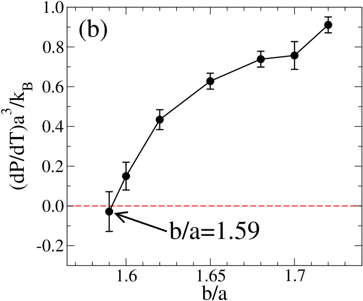
Figure 2: The LLCP, temperature of maximum density (TMD) line and the slope of the LDL-HDL coexistence line for a selection of modified Jagla potentials. (a) The critical point (solid symbols with error bar approximately the symbol size) and the TMD line (open symbols) for systems with $b/a=1.72,1.68,1.65,1.62,1.59$. One can see that the LLCP monotonically shifts to higher pressure and lower temperature as $b/a$ decreases. The density anomaly region bounded by the TMD line, expands in the $T$-$P$ diagram with decreasing $b/a$, and the LLCP moves from above the TMD line towards the density anomaly region and for $b/a=1.59$, the LLCP locates right on top of the TMD line. (b) The slope of the LDL-HDL coexistence lines decreases as the $b/a$ value decreases. When $b/a$ approaches $1.59$, the slope decreases to zero.

We first explore the phase diagram of each model with different $b/a$ via slow cooling using constant volume simulations. The LLCP corresponds to the highest temperature crossing of isochores in the $T$-$P$ phase diagram. The temperature of maximum density (TMD) line is the locus of state points at which pressure reaches a minimum along each isochore as a function of $T$ XuPRE2006 . Figure 2(a) shows that the LLCP monotonically shifts to lower temperature and higher pressure as $b/a$ decreases. The region of the density anomaly (the region bounded by the TMD line) expands and shifts together with the LLCP to higher pressures as $b/a$ decreases. This behavior coincides with the behavior reported in Ref. gibsonWilding . (The numerical differences in $P$ and $T$ arise from the fact that we define the unit of energy as $U_{0}\equiv-U_{A}$, while Ref. gibsonWilding uses $U_{0}\equiv U_{R}/0.69$.) When $b/a<1.59$ the system crystallizes spontaneously near the LLCP within a short simulation time, and we are not able to obtain the LLCP and coexistence line.

We calculate the slope of the LLPT coexistence line $dP/dT$ for systems with different $b/a$ [Fig. 2(b)] by the Maxwell construction. One can see that the slope decreases from positive to approximately zero as $b/a$ decreases to 1.59, in agreement with Ref. gibsonWilding . For large $b/a$, the LLCP lies clearly above the density anomaly region bounded by the TMD line, corresponding to the case of $dP/dT>0$, while for $b/a=1.59$, the LLCP lies on the TMD line corresponding to the case of $dP/dT=0$ [Fig. 2(a)]. Theoretically, if $dP/dT<0$, the LLCP should be inside the density anomaly region SastryPRE2006 , as is confirmed by the linear scaling theory, which we will address in detail in Sec. VI.

III.2 Widom line

For the first order phase transition, the order parameter, entropy, or density is discontinuous on crossing the coexistence line. At the critical point, where the coexistence line terminates, the critical fluctuations of $C_{P}$ and $K_{T}$ diverge, and show maxima in the one phase region close to the critical point. In this section, we study the behavior of $C_{P}$ maxima and $K_{T}$ maxima lines near the LLCP for models with different coexistence line slopes.

III.2.1 Isobaric specific heat $C_{P}$

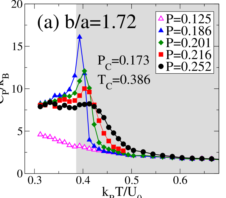
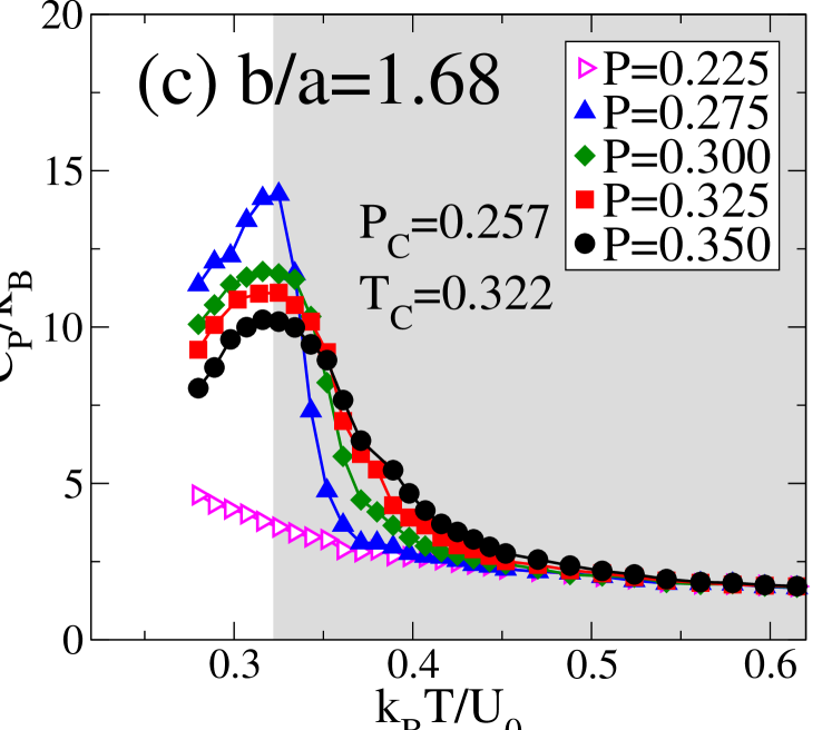
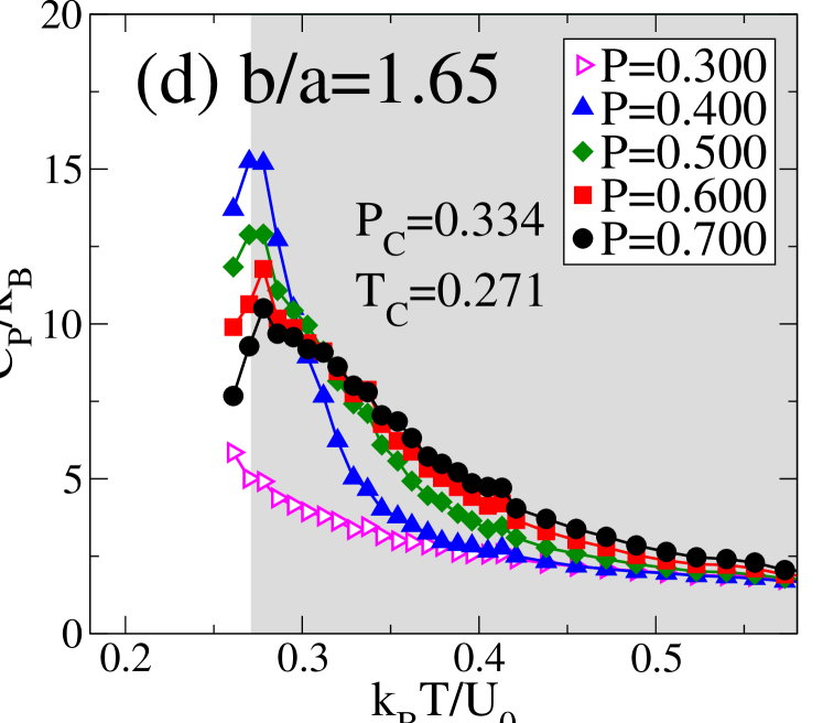
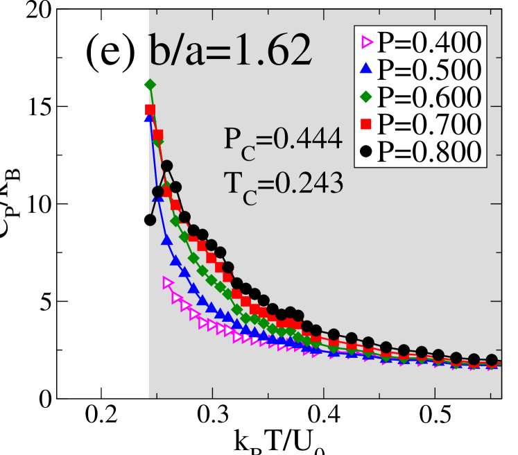
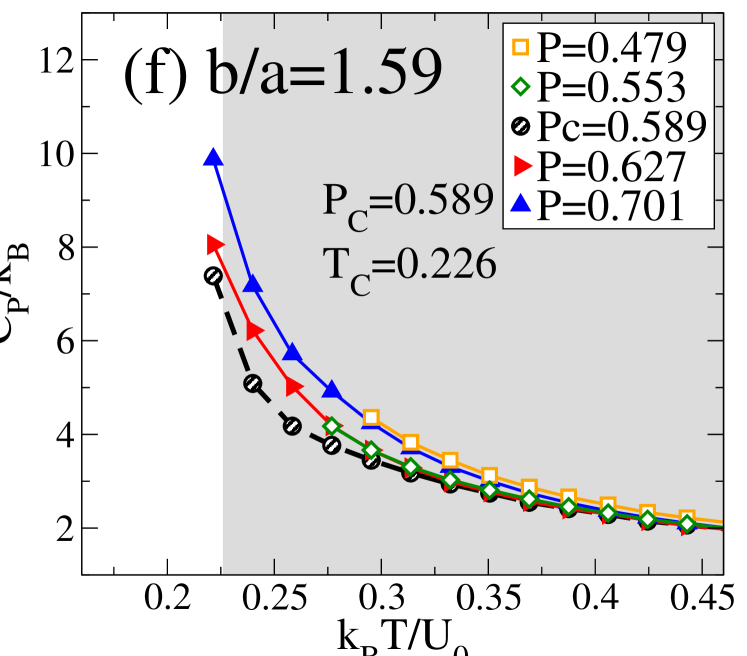
Figure 3: Specific heat $C_{P}$ for systems with different $b/a$. Only equilibrated results are shown. The gray area indicates the $T>T_{c}$ region. (a-d) For $b/a\geq 1.65$, one can see that $C_{P}$ shows maxima at pressures $P>P_{c}$, and as $P_{c}$ is approached, the increase in $C_{P}$ starts at lower $T$ but becomes sharper. As the pressure increases, the $C_{P}$ peak moves to higher $T$, indicating a positive slope of the $C_{P}$ maxima locus, which follows the coexistence line for these models. For pressure $P<P_{c}$, $C_{P}$ monotonically increases without any maximum. (e) For $b/a=1.62$, $C_{P}$ monotonically increases without showing any peak also for $P>P_{c}$, except at the highest pressure studied $P=0.800$. The system enters a glassy state at lower $T$ where no equilibrium data can be obtained. (f) For $b/a=1.59$ with horizontal coexistence line, no $C_{P}$ maxima can be found for the equilibrium states with $T\geq T_{c}$ for both $P>P_{c}$ and $P<P_{c}$.

We first explore the behavior of the $C_{P}$ maxima line for modified Jagla models with different $b/a$. For $b/a\geq 1.62$, the coexistence line has a positive slope [Fig. 2(b)]. Upon cooling along constant pressure above the critical pressure $P_{c}$ in the one-phase region, we observe peaks in $C_{P}$ for the cases $b/a=1.72$, 1.70, 1.68, and 1.65 [Fig. 3(a-d)]. As the LLCP is approached the magnitude of the $C_{P}$ peaks increases, and at the LLCP they diverge in an infinite system. When $P<P_{c}$, we observe a continuous increase in $C_{P}$ without any peak when the coexistence line is crossed. Thus we can locate the LLCP by locating the terminal point of the $C_{P}$ maxima line.

We note that the $C_{P}$ peaks move toward higher $T$ at higher $P$, indicating a positively sloped line [Fig. 3(a,b)]. This is consistent with the fact that the Widom line is the extension of the coexistence line into the one-phase region, and for these values of $b/a$ the coexistence line is positively sloped. However the slopes of the $C_{P}$ maxima lines increase as the slopes of the coexistence lines decrease and eventually, at $b/a=1.65$, the $C_{P}$ maxima line becomes nearly vertical, clearly showing that the $C_{P}$ maximum is no longer serving its original purpose, as will be explained in Sec. IV below. For $b/a=1.62$, $C_{P}$ monotonically increases without showing any peak for pressures $P>P_{c}$, except at the highest pressure studied $P=0.800$ [Fig. 3(e)].

When $b/a=1.59$ with a horizontal coexistence line, $C_{P}$ monotonically increases with decreasing $T$ along a constant pressure path both below and above $P_{c}$ [Fig. 3(f)]. When $b/a=1.62$, there are no $C_{P}$ maxima in the equilibrium region with $T\geq T_{c}$, but $C_{P}$ behaves symmetrically either below or above $P_{c}$.

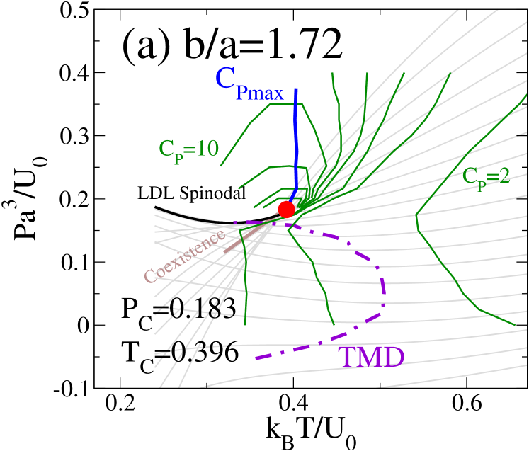
Figure 4: Phase diagram with specific heat $C_{P}$ for positively sloped coexistence line case ($b/a=1.72$) and horizontal coexistence line case ($b/a=1.59$). Isochores (solid gray), TMD line (dash purple), and LLCP (red solid circle) are shown. (a) $b/a=1.72$, the lines of equal $C_{P}$ (solid green), change from $C_{P}=2$ far away from the LLCP to $C_{P}=10$ close to the LLCP with interval $\Delta C_{P}=1$. $C_{P}$ maxima locus crosses the lines of equal $C_{P}$ at the points of their maximal pressure, and follows the coexistence line into the one-phase region, then sharply turns upwards to higher pressures and becomes almost vertical. (b) For $b/a=1.59$, the lines of equal $C_{P}$ (solid green), change from $C_{P}=2.0$ far away from the LLCP to $C_{P}=4.5$ close to the LLCP with interval $\Delta C_{P}=0.5$. No $C_{P}$ maxima can be observed before the system either goes into glassy states or crystallizes. However, one notes that the $C_{P}$ is symmetric with respect to the critical pressure.

We plot the lines of equal $C_{P}$ for two extreme cases, $b/a=1.72$ with a positively sloped coexistence line [Fig. 4(a)] and $b/a=1.59$ with a horizontal coexistence line [Fig. 4(b)]. When $b/a=1.72$, the lines of equal $C_{P}$ form loops in the $T$-$P$ plane and cross the $C_{P}$ maxima line at their maxima points. The locus of $C_{P}$ maxima extends the coexistence line into the one-phase region in the vicinity of the critical point. Then it sharply turns upwards to higher pressures and becomes approximately vertical. For $b/a=1.59$, there are no $C_{P}$ maxima. The equal $C_{P}$ lines extend away from the critical point symmetrically without any loops. At low $T$, we reach the simulation limit due to either crystallization for $P<P_{c}$ or due to entering a glassy state for $P>P_{c}$, where no equilibrium results can be obtained for the analysis.

We note that the magnitude of $C_{P}$ drops significantly when the coexistence line is horizontal with $b/a=1.59$, compared to when $b/a=1.72$. This is because, when the coexistence line is horizontal, the difference in enthalpy $H$ between LDL and HDL is zero according to the Clapeyron equation of thermodynamics,

$$\frac{dP}{dT}=\frac{\Delta H}{T\Delta V}$$ (6)

In this case, the enthalpy fluctuations that determine the magnitude of the specific heat gain no strength from the critical fluctuations, except from the weak $PV$ term.

III.2.2 Isothermal compressibility $K_{T}$

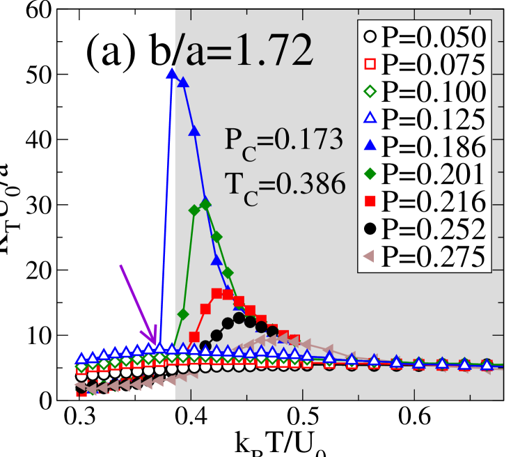
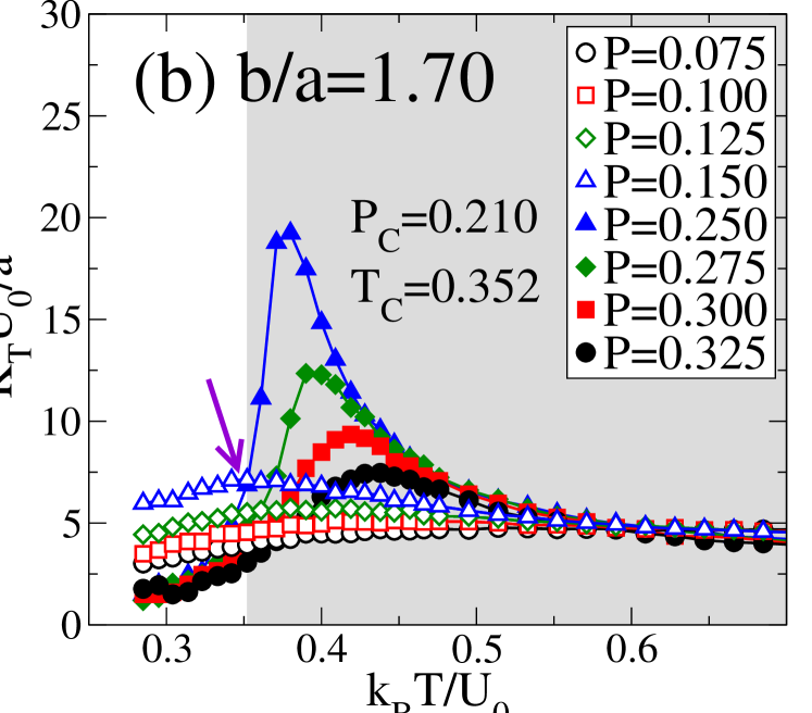
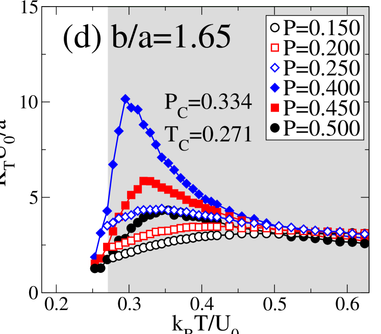
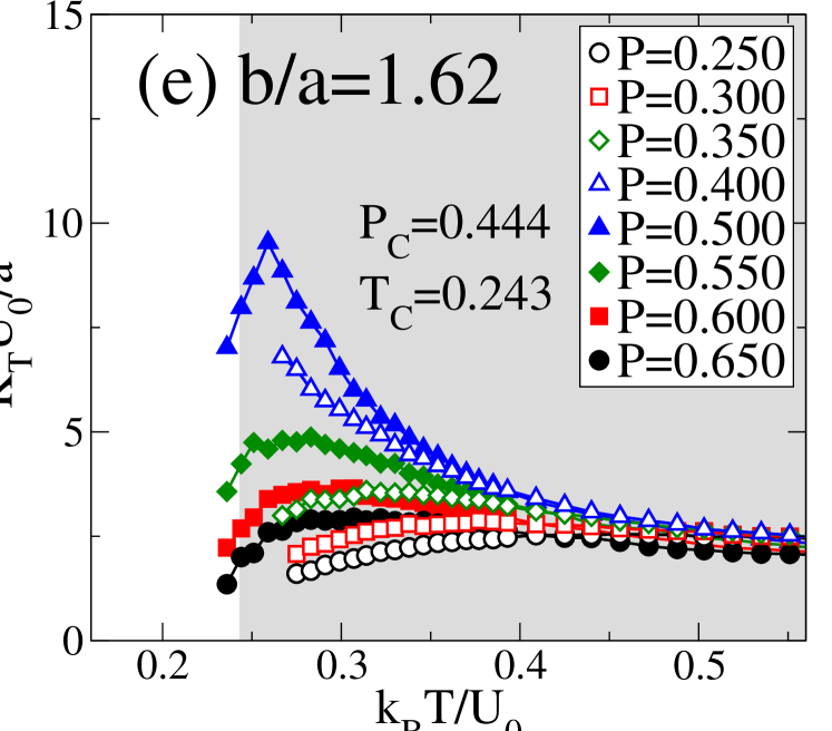
Figure 5: Compressibility $K_{T}$ for models with different $b/a$. The maxima in $K_{T}$ both for $P<P_{c}$ (open symbols) and for $P>P_{c}$ (solid symbols with arrows pointing to the peaks) are shown. (a-e) For $b/a\leq 1.62$,the magnitudes of $K_{T}$ for $P>P_{c}$ are much larger than for $P<P_{c}$. The maxima for $P>P_{c}$ correspond to critical fluctuations, while the maxima for $P<P_{c}$ correspond to the approach to the LDL spinodal. (f) For $b/a=1.59$, with the horizontal coexistence line, the $K_{T}$ below and above $P_{c}$ are almost identical, with equal magnitudes of their maxima.

Figure 5 shows the behavior of $K_{T}$ above and below $P_{c}$ and contrasts it with that of $C_{P}$. For $b/a\geq 1.62$, when the coexistence line slope is positive, $K_{T}$ shows maxima both above and below $P_{c}$. For $P>P_{c}$ in the one-phase region, similar to $C_{P}$, the $K_{T}$ peaks become more prominent as the LLCP is approached [Fig. 5(a–e)]. For a finite system, $K_{T}$ diverges at the LLCP. For $P<P_{c}$, we observe a second set of $K_{T}$ peaks with much lower magnitudes. For $b/a=1.59$ with a horizontal coexistence line, $K_{T}$ behaves symmetrically above and below $P_{c}$, with equal magnitudes of the maxima [Fig. 5(f)].

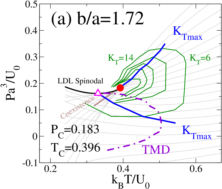
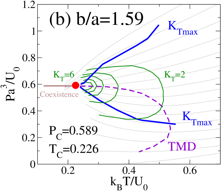
Figure 6: Phase diagram with compressibility $K_{T}$ for positively sloped coexistence line case with $b/a=1.72$ and horizontal coexistence line case with $b/a=1.59$. (a) For $b/a=1.72$, the lines of equal $K_{T}$ (solid green), changes from $K_{T}=6$ far away from the LLCP to $K_{T}=14$ close to the LLCP with interval $\Delta K_{T}=2$. One can see that the loci of the two $K_{T}$ maxima cross the lines of equal $K_{T}$ at points of their maximal and minimal pressures, and are not symmetric with respect to $P_{c}$. The locus with higher magnitude of $K_{T}$ maxima, which corresponds to the critical fluctuations, merges to the LLCP. The locus with the lower magnitude of $K_{T}$ maxima extends below $T_{c}$, and terminates at the minimum pressure point of the LDL spinodal (triangle symbol), where the TMD line also terminates. This brunch of $K_{T}$ maxima also crosses the TMD line at the point of its maximal temperature. (b) For $b/a=1.59$, the lines of equal $K_{T}$ (solid green), changes from $K_{T}=2$ far away to $K_{T}=6$ close to the LLCP with interval $\Delta K_{T}=1$, The loci of equal $K_{T}$ form symmetric loops around the LLCP, and both $K_{T}$ maxima lines merge to the LLCP with equal magnitudes of their maxima.

Figure 6 shows the loci of $K_{T}$ maxima for both $b/a=1.72$ with a positive coexistence line slope and $b/a=1.59$ with a horizontal coexistence line. For $b/a=1.72$, the values of the $K_{T}$ maxima at $P>P_{c}$, which corresponds to the critical fluctuations and originates from the LLCP, have a much larger magnitude than the values of $K_{T}$ maxima at $P<P_{c}$. The second $K_{T}$ maxima line at $P<P_{c}$ corresponds to the approach to the LDL spinodal and terminates at the lowest pressure point of the LDL spinodal where the TMD line also terminates XuJCP2009 ; sergeyReview . Furthermore, the $P<P_{c}$ $K_{T}$ maxima line also crosses the TMD line at the point of its maximal temperature SastryPRE2006 . Similar to $C_{P}$, the lines of equal $K_{T}$ form loops, and cross at their maximal pressure points with the $P>P_{c}$ and $P<P_{c}$ $K_{T}$ maxima lines. For $b/a=1.59$ [Fig. 6], the lines of equal $K_{T}$ form symmetric (with respect to $P_{c}$) loops around the critical point. Both $K_{T}$ maxima lines merge at the LLCP.

In the case of $b/a=1.72$, from both Fig. 4 and Fig. 6, we can identify the Widom line as the overlapping segment of the $C_{P}$ maxima and the $K_{T}$ maxima lines, which extends the coexistence line into the one-phase region in the vicinity of the LLCP. In contrast, for $b/a=1.59$ with a horizontal coexistence line, the $C_{P}$ maxima line disappears, where the specific heat $C_{P}$ can no longer be a good representative for critical fluctuations. Indeed, there is no enthalpy difference between the two coexisting phases, so there can be no contribution to enthalpy fluctuations from the critical fluctuations. However, the density fluctuations remain well defined, with two $K_{T}$ maxima lines above and below the critical pressure, both associated with the critical fluctuations. In the vicinity of the critical point, the two $K_{T}$ maxima lines merge together and can be used to locate the critical point from measurements obtained in the supercritical region only.

IV Comparison with the linear scaling theory of the liquid-liquid critical point

To explain the change of behavior of the lines of response function extrema for the horizontal coexistence line case, we adapt the linear scaling theory of the liquid-liquid critical point developed by M. A. Anisimov and collaborators AnisimovPRE .

The field-dependent thermodynamic potential $\psi$ can be considered a universal function of two scaling fields: “ordering” $h_{1}$ and “thermal” $h_{2}$. Near the critical point $\psi$ can be written

$$\psi\simeq h^{2-\alpha}_{2}f(\frac{h_{1}}{h^{\beta+\gamma}_{2}}),$$ (7)

where the critical exponents have the values for the Ising universality class, $\alpha=0.109$, $\beta=0.326$, and $\gamma=1.239$ AnisimovPRE .

Since our focus is on the immediate vicinity of the liquid-liquid critical point, we neglect the curvature of the coexistence line and the background contribution to the response functions. We assume the scaling fields are linear analytical combinations of physical fields, the pressure $P$, and the temperature $T$,

$$h_{1}=a_{1}\Delta\hat{P}+a_{2}\Delta\hat{T},$$ (8)

$$h_{2}=b_{1}\Delta\hat{T}+b_{2}\Delta\hat{P}.$$ (9)

with $\Delta\hat{P}\equiv(P-P_{c})/(\rho_{C}RT_{c})$ and $\Delta\hat{T}\equiv(T-T_{c})/T_{c}$, where the subscript “$c$” here and below indicates the critical parameters, and $a_{i}$ and $b_{i}$ are system-dependent coefficients.

We introduce a tuning parameter $\phi$ into the theory, and we use it to change the slope of the coexistence line by defining

$$a_{1} \equiv \cos\phi,\ \ a_{2}\equiv-\sin\phi,$$

$$b_{1} \equiv \cos\phi,\ \ b_{2}\equiv\sin\phi.$$ (10)

Then the slope of the coexistence line is

$$\frac{dP}{dT}=\tan\phi.$$ (11)

The critical (fluctuation-induced) parts of the dimensionless isobaric specific heat and isothermal compressibility are expressed through the scaling susceptibilities AnisimovPRE

$$(\hat{C}_{P}) = \hat{T}(\frac{\partial\hat{S}}{\partial\hat{T}})_{\hat{P}}$$ (12)

$$= \hat{T}(\sin^{2}\phi\chi_{1}-\sin 2\phi\chi_{12}+\cos^{2}\phi\chi_{2}),$$

$$(\hat{K}_{T}) = -\frac{1}{\hat{V}}(\frac{\partial\hat{V}}{\partial\hat{P}})_{\hat{T}}$$ (13)

$$= \frac{1}{\hat{V}}[\cos^{2}\phi\chi_{1}-\sin 2\phi\chi_{12}+\sin^{2}\phi\chi_{2}],$$

$$(\hat{\alpha}_{P}) = \frac{1}{\hat{V}}(\frac{\partial\hat{V}}{\partial\hat{T}})_{\hat{P}}$$ (14)

$$= \frac{1}{\hat{V}}(\frac{1}{2}\sin 2\phi\chi_{1}-\cos 2\phi\chi_{12}-\frac{1}{2}\sin 2\phi\chi_{2}).$$

where $\hat{T}=T/T_{c}$, $\hat{P}=P/\rho_{C}RT_{c}$.

The scaling fields and scaling susceptibilities can be written as functions of the “polar” variables $r$ and $\theta$, and two constants $a$ and $k$, which can be obtained by fitting the experimental data,

$$h_{1}=ar^{\beta+\gamma}\theta(1-\theta^{2}),$$ (15)

$$h_{2}=r(1-b^{2}\theta^{2}),$$ (16)

$$\chi_{1}=\frac{k}{a}r^{-\gamma}c_{1}(\theta),$$ (17)

$$\chi_{12}=kr^{\beta-1}c_{12}(\theta),$$ (18)

$$\chi_{2}=akr^{-\alpha}c_{2}(\theta),$$ (19)

where

$$c_{1}(\theta)=[1-b^{2}\theta^{2}(1-2\beta)]/c_{0}(\theta),$$ (20)

$$c_{12}(\theta)=\beta\theta[1-\delta-\theta^{2}(3-\delta)]/c_{0}(\theta),$$ (21)

$$c_{2}(\theta)=[(1-\alpha)(1-3\theta^{2})s(\theta)-2s_{2}\beta\delta\theta^{2}(1-\theta^{2})]/c_{0}(\theta),$$ (22)

$$c_{0}(\theta)=(1-3\theta^{2})(1-b^{2}\theta^{2})+2\beta\delta b^{2}\theta^{2}(1-\theta^{2}).$$ (23)

Here $b=\sqrt{(\gamma-2\beta)/\gamma(1-2\beta)}=1.16679$, $\delta=\gamma/\beta+1=4.80061$, and $s(\theta)$ are known functions,

$$s(\theta)=s_{0}+s_{2}\theta^{2},$$ (24)

$$s_{0}=-(2-\alpha)f_{0},$$ (25)

$$s_{2}=-(2-\alpha)b^{2}(1-2\beta)f_{0}-\gamma f_{2},$$ (26)

with

$$f_{0}=-\frac{\beta(\delta-3)-b^{2}\alpha\gamma}{2b^{4}(2-\alpha)(1-\alpha)\alpha},$$ (27)

$$f_{2}=\frac{\beta(\delta-3)-b^{2}\alpha(1-2\beta)}{2b^{2}(1-\alpha)\alpha}.$$ (28)

Since all response functions are directly propositional to $k$, its actual value is irrelevant for our study. The value of $a$ determines the strength of the ordering field. We found that for large values of $a$, the overlapping segments of $C_{P}$ and $K_{T}$ maxima lines are shorter, which more adequately models the behavior of our simulations.

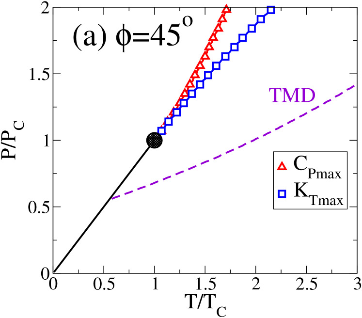
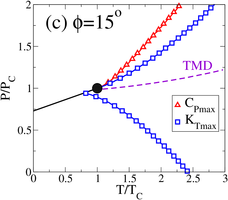
Figure 7: $C_{P}$ maxima and $K_{T}$ maxima obtained from the linear scaling theory of the critical point with $\phi=45^{o},30^{o},15^{o},0$. The coexistence line (solid black) has the slope $dP/dT=\tan\phi$. One can see that for more positively sloped coexistence line with larger $\phi$, at $P>P_{c}$, $C_{P}$ maxima and $K_{T}$ maxima lines have longer overlapping segments. while for smaller $\phi$, the merged section is shortened, and disappears (no overlapping) when $\phi=0$, with a horizontal coexistence line. The second $K_{T}$ maxima line at $P<P_{c}$ corresponding to the LDL spinodal can be seen for $\phi=30^{o}$ and $15^{o}$. Due to the lack of metastability of the states in the theory, the $K_{T}$ maxima at $P<P_{c}$ terminates at the coexistence line, instead in reality, it terminates at the minimum pressure point of the LDL spinodal. For $\phi=0$ with horizontal coexistence line, a second $C_{P}$ maxima line at $P<P_{c}$ merge to the LLCP. As we know, the linear scaling theory can predict the critical phenomena only close to the LLCP, a closer study near the LLCP will follow. Further, the TMD line (dash) is also shown, which is the locus of $\alpha_{P}=0$. One notices that as the slope of coexistence line goes from positive to horizontal, the TMD line shifts from being below the LLCP, to right on top of it, which is consistent with our results in DMD simulation. Here $a=0.47$, and $k=0.47$.

We study the behavior of $C_{P}$ and $K_{T}$ in systems with different coexistence line slopes. Figure 7 shows a plot of the loci of $C_{P}$ and $K_{T}$ maxima in the $T$-$P$ plane. Note that both the locus of $C_{P}$ maximum and the $K_{T}$ maxima line with the higher magnitude originate from the LLCP, and coincide with each other close to the LLCP before they separate. The locus of $C_{P}$ maximum bends towards a lower temperature than that of the $K_{T}$ maximum line. As the slope of the coexistence line decreases, the overlapping segments of the loci of $C_{P}$ and $K_{T}$ maxima shorten. When the coexistence line is horizontal, the loci of $C_{P}$ and $K_{T}$ maxima separate.

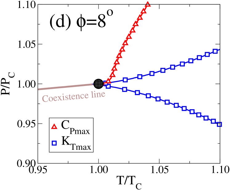
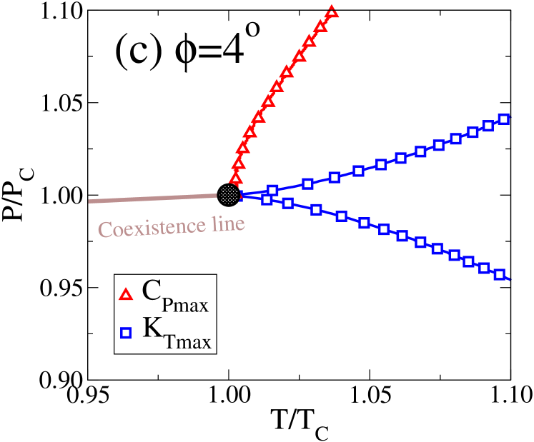
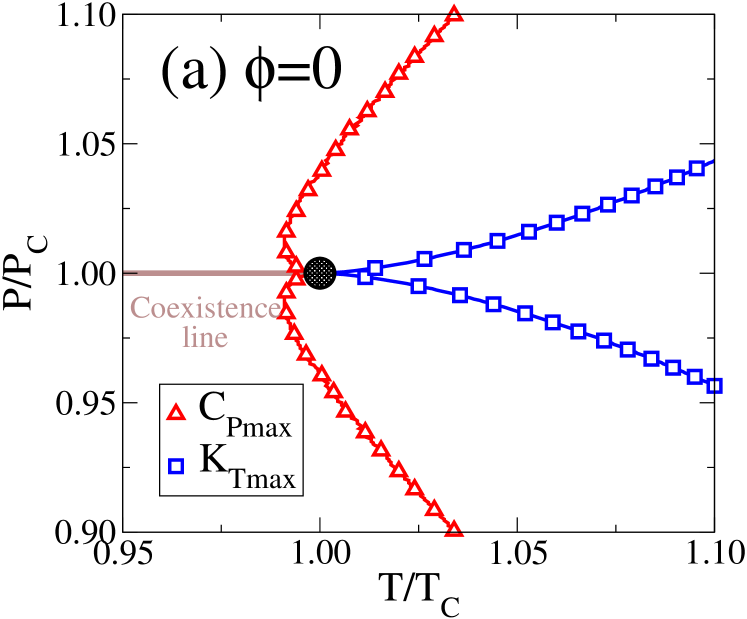
Figure 8: $C_{P}$ maxima and $K_{T}$ maxima loci on $T$-$P$ plane obtained from the linear scaling theory of the critical point, with small $\phi=8^{\circ},4^{\circ},6^{\circ},0$. One can see that as we decrease $\phi$, with the slope of coexistence line approaching zero, the $K_{T}$ maxima locus changes are not significant, while the $C_{P}$ maxima become more and more vertical. For a horizontal slope, two $C_{P}$ maxima lines converge at $T<T_{c}$ and enter the LLCP horizontally from below. There is no overlapping between $K_{T}$ maxima and $C_{P}$ maxima lines. Here we use $a=2$, and $k=1$, which is good to present the small or zero coexistence line case.

We then examine the systems with the slope of coexistence line very close to zero with small $\phi$ as shown in Fig. 8. We see that the loci of $K_{T}$ maxima are similar, with two $K_{T}$ maxima lines approaching the LLCP from $T>T_{c}$, but the $C_{P}$ maxima line deviates from the $K_{T}$ maxima lines and its slope becomes more vertical, as the slope of the coexistence line approaches zero. For the horizontal coexistence line, a second $C_{P}$ maxima line emerges, and converges with the first $C_{P}$ maxima line at $T<T_{c}$. Both of the $C_{P}$ maxima lines enter the critical point almost horizontally from $T<T_{c}$, while the $K_{T}$ maxima lines enter from $T>T_{c}$ horizontally. Thus in this case, close to the LLCP at $T\geq T_{c}$, no $C_{P}$ maxima can be found. According to the linear scaling theory, the actual $C_{P}$ maxima may exist below $T_{c}$ where, in our simulations, they are buried in the crystallization region or in glassy states with no equilibrium data for analysis. Further, there is no convergent behavior of the $C_{P}$ maxima and $K_{T}$ maxima near the LLCP in the horizontal coexistence line case. The Widom line, approximated by the locus of density fluctuation maxima, is the convergent loci of the $K_{T}$ maxima, while the identification of the Widom line using the $C_{P}$ maxima is no longer a fruitful method.

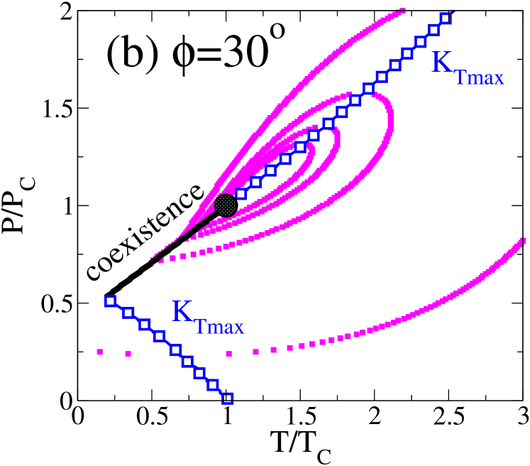
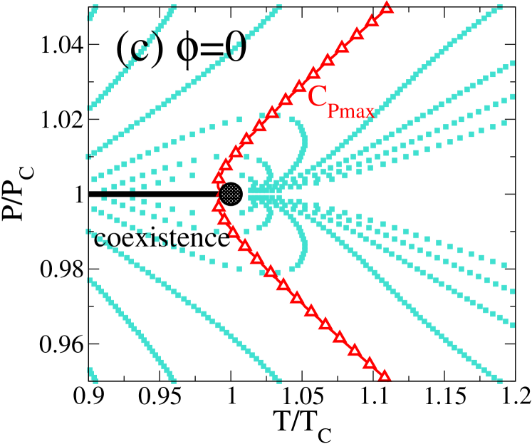
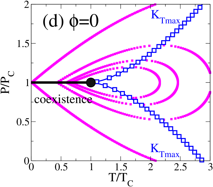
Figure 9: Comparison of $C_{P}$ and $K_{T}$ from linear scaling theory of the critical point. (a,b) $C_{P}$ and $K_{T}$ for the positively sloped coexistence line with $\phi=30^{o}$, respectively. The lines of equal $C_{P}$ and $K_{T}$ are shown. Both $C_{P}$ and $K_{T}$ contours loop around LLCP, with the locus of the maxima follow the coexistence line into the one-phase region. (c,d) $C_{P}$ and $K_{T}$ for the horizontal coexistence line with $\phi=0$, respectively. One can see that $C_{P}$ and $K_{T}$ are both symmetric below and above $P_{c}$. For clarity, (c) displays a narrow vicinity of the LLCP. Here we choose $a=0.47$, and $k=0.47$.

We also find out that when the slope of the coexistence line is positive, the contours of $C_{P}$ and $K_{T}$ go around the LLCP, with the pressure maxima following the extension of the coexistence line into the one-phase region [Fig. 9(a-f)]. When the slope of coexistence line is horizontal, there are symmetric contours above and below the critical pressure. This matches well with what we find in our simulation [Figs. 4 and 6].

V Glass transition

By decreasing the $b/a$ ratio, the LLCP is pushed into a metastable region with respect to crystallization, where the system is close to the glass transition (GT). We hence investigate the relationship between LLPT and GT in systems with different slopes of coexistence line.

While the inability to equilibrate in this domain was noted by Gibson and Wilding in their seminal study gibsonWilding , they did not discuss the “glass transition” (which is not a true transition in the thermodynamic sense). The GT is a concept useful for describing the manner in which viscous liquid systems fall out of equilibrium on cooling, or regain it during heating. It is better described as a “glass transformation zone” within which the system is neither fully arrested nor fully equilibrated. It may be studied in simulation, as it is in the laboratory OguniJCP1983 , by “scanning calorimetry.” In scanning calorimetry the enthalpy is monitored continuously as the system attempts, and increasingly succeeds, to explore all its degrees of freedom as temperature rises from low values where all motions except vibrations are frozen out Angell95sr . Typically the range of temperature over which the transition extends is the range needed to change the relaxation time by two orders of magnitude, so it depends on the temperature dependence of the relaxation time Angell83jcp . Being kinetic in nature, this transition is hysteretic, as seen in our simulations. While it is usually studied by scanning calorimetry, it can equally be studied by volumetric methods.

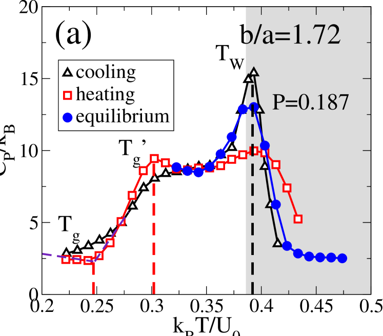
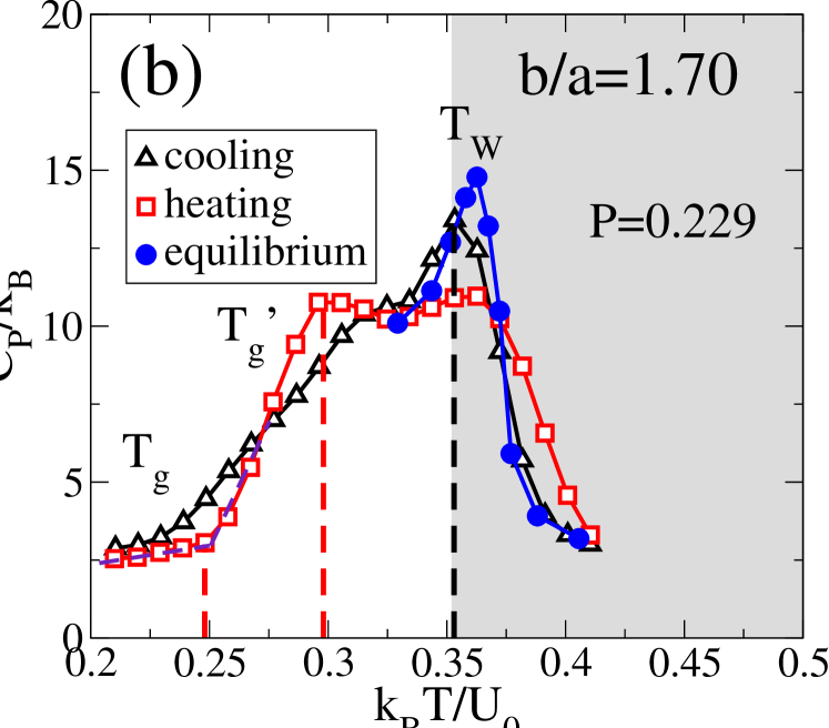
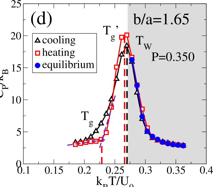
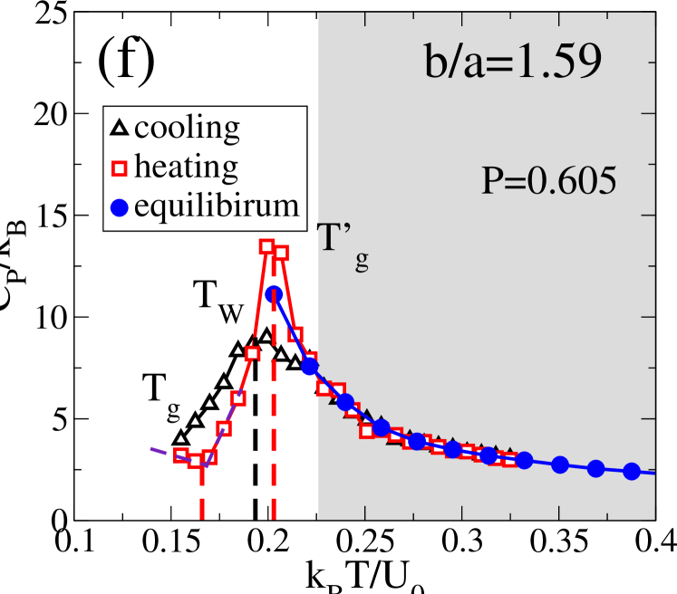
Figure 10: The comparison of $C_{P}$ upon slow cooling and heating for a selection of modified Jagla models. The cooling/heating rate is $q_{c}=q_{h}=10^{-6}q_{0}$. An isobaric path is selected at $P$ closely above $P_{c}$ in the one-phase region. The equilibrium values of $C_{P}$ are also plotted for comparison. The gray area is the temperature region for $T\geq T_{c}$. (a-c) For $b/a=1.72,1.70$ and $1.68$, two peaks of $C_{P}$ upon heating can be observed. The high temperature peak $T_{W}$, arising from the presence of the Widom line, is related to the LLPT. The low temperature peak upon heating, $T^{\prime}_{g}$, corresponds to the ergodicity restoration slightly above the glass transition $T_{g}$ obtained from standard construction (dash line). One can see that the distance between the glass transition peak $T^{\prime}_{g}$/$T_{g}$ and $T_{W}$ decreases as the $b/a$ value decreases, with the LLCP moving closer to the glass transition. (d-f) For $b/a=1.65,1.62$ and $1.59$, upon heating, only one peak of $C_{P}$ can be observed, and this peak shifts below $T_{c}$, while for other cases it is well above $T_{c}$. One also notices that system shows a prominent $K_{T}$ peak in the studied $P$ region (Fig. 5). In these models with small coexistence line slope, the enthalpy fluctuations play less role in the critical fluctuations, while the density fluctuations is the leading term. And as the LLCP being pushed closer to $T_{g}$, the critical fluctuations become suppressed by the glass transition, where $C_{P}$ only shows one peak upon heating.

The glass temperature $T_{g}$ can be defined as the point at which the uptake of configurational enthalpy begins to commence (onset $T_{g}$, the value usually reported by experimentalists), or the temperature at which equilibrium (ergodicity) is fully restored, $T^{\prime}_{g}$. Each is defined diagrammatically in Fig. 10, the distance between the two amounting to about $25\%$ of the absolute value. It is a much more diffuse phenomenon than in the laboratory where the width is only $5\%$ of the absolute value (due to the increased temperature dependence of the relaxation time near the laboratory $T_{g}$) Angell83jcp .

We estimate $T_{g}$ and $T^{\prime}_{g}$, as in the laboratory experiment, by plotting the derivative of the enthalpy (apparent specific heat), during cooling and heating the systems through GT along isobars slightly above the critical pressure $P_{c}$, at constant cooling/heating rate $q_{c}=q_{h}=10^{6}q_{0}=10^{7}$K/sec [Fig. 10]. We find that for upscans in the positively sloped coexistence line case ($b/a=1.72$), $C_{P}$ shows two well-separated peaks [Fig. 10(a)]. The high temperature peak $T_{W}$, is related to the fluctuations associated with the LLPT and is used to locate the Widom line. The second peak (at the lower temperature $T=T^{\prime}_{g}$) is an “overshoot” phenomenon due to ergodicity restoration kinetics. It is seen in most laboratory systems (but not polymers) and is not observed during cooling, (a measure of the hysteretic character of the glass transition). The lower $T_{g}$ is obtained from the standard construction (dashed line) AngellScience2008 .

Similar well-separated $T_{W}$ and $T^{\prime}_{g}$ peaks can be observed for $b/a=1.70$, and $1.68$ [Fig. 10(b,c)], but the temperature difference between the two peaks shrinks as the $b/a$ value decreases. When $b/a<1.68$, the “normal” and critical fluctuations merge because of the similarity in their time scales, but study of the density fluctuations as reflected in the compressibility of Fig. 5 shows that indeed $T_{c}>T_{g}$, and the critical point is not suppressed by the kinetics of “background” enthalpy fluctuations (as the collected data in Fig. 10 might imply at first sight). Rather, what is happening is that the critical fluctuations in enthalpy are losing their thermodynamic strength due to the vanishing of any enthalpy difference between the alternative phases that is dictated by the Clapeyron equation for horizontal coexistence lines (see Fig. 2 for $b/a=1.59$). Thus, at $b/a=1.59$, the apparent specific heat plot, notwithstanding the proximity of the critical point, is indistinguishable in character from that previously reported for the glass transition of the low density liquid at pressures well below $P_{c}$ in the earlier study of Xu et al. XuJCP2009 .

Figure 11 shows that the critical fluctuation domain becomes increasingly related to the slow (glassy) dynamics domain as the repulsive potential becomes steeper (second length scale approaches the first, more closely as $b/a$ decreases). It is unfortunate that the increase of the equilibrium melting point, in the same $b/a$ range, throws the system into conflict with still another, and faster kinetics, that of crystal nucleation, so that the relation between the first two can no longer be followed for smaller $b/a$.

Just as the mixing of Lennard-Jones (LJ) particles has made possible the study of supercooled and glassy states of LJ, so might the mixing of Jagla particles of different dimensions and attractive well depths, make possible more extended studies of the critical point/glass temperature relations. Note that in the glass-forming LJ mixtures there is no suggestion of stable domain critical points, though specific heats in excess of vibrational values do increase sharply as temperature decreases.

As a final remark, it is notable that the strengths of the response functions specific heat and compressibility in laboratory molecular glassformers also vary in opposite directions as $T_{g}$ is approached, the case of o-terphenyl being the best documented so far AngellNaturePhys2011 . The relationship is similar to that of the response functions maxima for the present model at small $b/a$ demonstrated in Figure  3 and  5 showing that there is a temperature interval near the glass transition where $C_{P}$ is increasing upon cooling while the $K_{T}$ decreasing, with the only difference that there is no stable second critical point in the laboratory case.

VI Summary and Conclusions

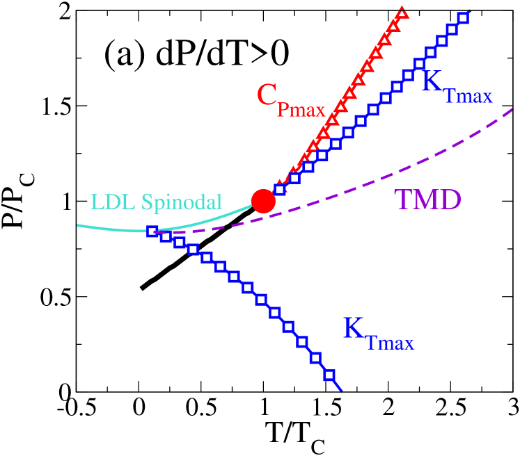
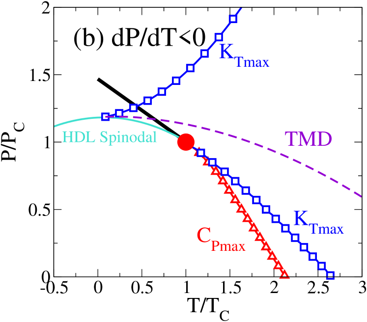
Figure 12: The relationship between the slope of the coexistence line and the behavior of the Widom line and the TMD line. (a) For the case of positively sloped coexistence line, the $C_{P}$ maxima line originates from the LLCP and extends into the one-phase region as a continuation of the coexistence line, while the $K_{T}$ shows two maxima lines. One $K_{T}$ maxima line is related to critical fluctuations, and originates from the LLCP, coinciding with the $C_{P}$ maxima line in the vicinity of the critical point forming the Widom line. The other $K_{T}$ maxima line corresponds to the approach to the LDL spinodal, which terminates at the LDL spinodal at its lowest pressure point, where the TMD line also terminates (triangle symbol). (b) For the case of negatively sloped coexistence line, the phase diagram is similar to the mirror image of the positively sloped coexistence line case, with $C_{P}$ and $K_{T}$ maxima lines originating from the LLCP and extending into the one-phase region, and overlapping in the vicinity of the critical point. The second $K_{T}$ maxima line goes above the pressure of the critical point, and terminates at the HDL spinodal, where the TMD line also terminates. We note that in both cases, both $K_{T}$ extrema lines form a loop in the $T$-$P$ plane, which intersects the TMD line at its maximum temperature point of the TMD line (not shown). In case (a) the critical point lies outside the density anomaly region while in case (b) it lies inside the density anomaly region. Both graphs are constructed using the linear scaling theory of critical point with $\alpha=k=0.47$, and $\phi=25^{0}$ and $-25^{0}$, respectively. The lines of the spinodals are drawn as interpolation between the critical point and the extrapolated crossing point of the TMD and $K_{T}$ maxima lines beyond the coexistence line.

We have investigated the loci of the response function maxima in systems with different coexistence line slopes. We find that for the case of positively sloped coexistence line, the $C_{P}$ maxima line originates from the LLCP and extends into the one-phase region as a continuation of the coexistence line, while compressibility $K_{T}$ shows two maxima lines [Fig. 12(a)]. One of the $K_{T}$ maxima lines is related to critical fluctuations, and originates from the LLCP, coinciding with the $C_{P}$ maxima line in the vicinity of the critical point following the Widom line. This offers us a method to locate the LLCP from the high temperature side by tracking the $C_{P}$ maxima line, instead of tracking the coexistence line from the low temperature side where crystallization and glass transition bring huge experimental obstacles. The other $K_{T}$ maxima line is due to the approach to the LDL spinodal, and terminates at the LDL spinodal at its lowest pressure point, where the TMD line also terminates.

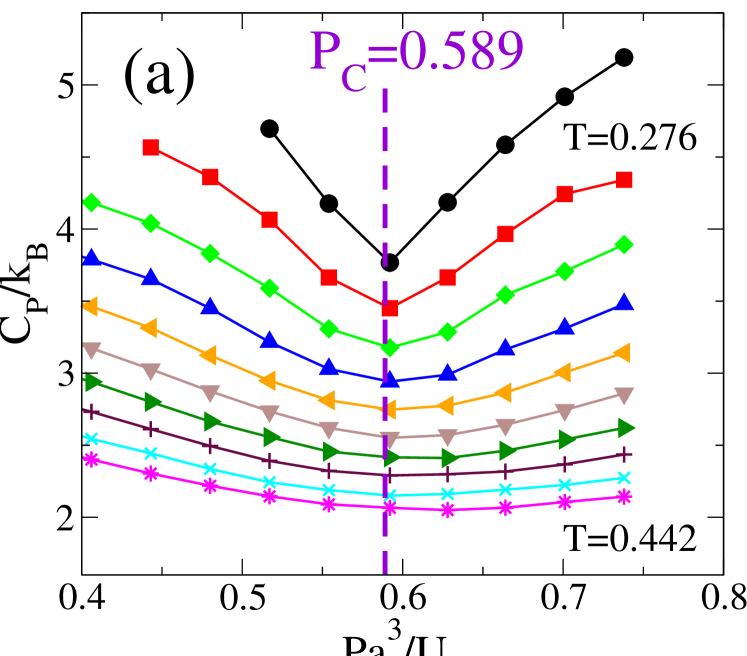
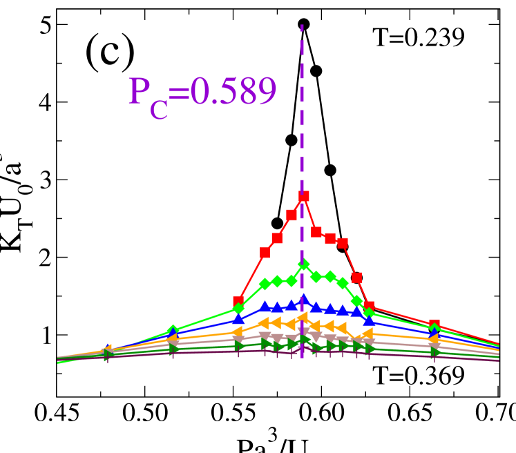
Figure 13: The behavior of $C_{P}$ and $K_{T}$ along different isotherms as functions of $P$ in simulations with a horizontal coexistence line $b/a=1.59$ (a,c), and the linear scaling theory with $\phi=0$ (b,d). (a) $C_{P}$ in simulations, $T$ changes from $0.276$ to $0.442$ with interval $\Delta T=0.180$, above $T_{c}=0.226$. (b) $C_{P}$ from linear scaling theory. Both results agree well with each other, that $C_{P}$ shows a minimum at $P_{c}$ for all temperatures, and as $T\rightarrow T_{c}$, the minimum value of $C_{P}$ increases, and the valley of the minimum gets narrower. This offers a way to track the critical point by isotherms at equilibrium temperatures, instead of isobar cooling into lower temperature. (c) $K_{T}$ in simulations, $T$ changes from $0.239$ to $0.369$ with interval $\Delta T=0.180$, above $T_{c}=0.226$. (d) $K_{T}$ from linear scaling theory. Again, the theory is consistent with the simulation results, that showing $K_{T}$ has maxima at $P_{c}$ for all temperatures and, as $T\rightarrow T_{c}$, the maximum value of $K_{T}$ increases and the peak gets sharper.

As the slope of coexistence line approaches zero, $C_{P}$ maxima disappears in the equilibrium region with $T\geq T_{c}$ [Fig. 12(b)]. However, along a constant temperature path, $C_{P}$ shows a minimum at the critical pressure $P_{c}$ [Fig. 13]. This is experimentally observed in water for which $C_{P}$ decreases with increasing pressure OguniJCP1983 . Hence, for a system with horizontal coexistence line, the LLCP can still be found by the $C_{P}$ minimum as function of $P$ at constant $T$. For $K_{T}$, both of the $K_{T}$ maxima lines as functions of $T$ are related to critical fluctuations, and start from the LLCP and extend symmetrically above and below $P_{c}$. In addition, a third $K_{T}$ maxima line as a function of $P$ at constant $T$ can be defined. All these three $K_{T}$ maxima lines converge at the LLCP, and together with the $C_{P}$ minimum line, can be used to locate the LLCP. Since in case of coexistence line with zero slope, the thermal field practically consides with temperature, this third $K_{T}$ maxima line gives the best approximation for the Widom line.

For negatively sloped coexistence line, the phase diagram near the critical point is similar to the phase diagram for the positively sloped coexistence line case reflected with respect to critical pressure $P=P_{c}$. This follows from the linear scaling theory of the critical point since according to Eq. (14) $K_{T}(-\phi,-\theta)=K_{T}(\phi,\theta)$, $C_{P}(-\phi,-\theta)=C_{P}(\phi,\theta)$, while $\alpha_{P}(-\phi,-\theta)=-\alpha_{P}(\phi,\theta)$, which comes from the symmetry of the functions with $\chi_{i}(\theta)$, $\chi_{1}(\theta)$, and $\chi_{2}(\theta)$ being even, but $\chi_{12}(\theta)$ being odd. The $C_{P}$ maxima line and one of the $K_{T}$ maxima lines both originate from the LLCP and extend into the one-phase region, while overlapping with each other in the vicinity of the critical point [Fig. 12(b)]. The second $K_{T}$ maxima line goes above the pressure of the critical point, and terminates at the point of maximum pressure of the HDL spinodal, where the TMD line also terminates.

Note that the location of the critical point with respect to the TMD line is related to the slope of the coexistence line. When the slope of the coexistence line is positive, the critical point stays outside the density anomaly region; when it is negative, the critical point is inside the density anomaly region; when it is horizontal, the TMD line terminates right at the LLCP [Fig. 12]. Indeed, when the slope is positive, the volume of the low temperature phase is smaller than the volume of the high temperature phase. Thus if we connect these two phases by the isobar with $P>P_{c}$, the volume along this isobar decreases with $T$, the region above the critical point corresponds to the $\alpha_{P}>0$ and, because $\alpha_{P}$ is a continuous function everywhere except at the LLCP, $\alpha_{P}$ also remains positive in the one-phase region for pressure below the LLCP. Accordingly, the LLCP lies outside the region of density anomaly. Analogous considerations show that, when the slope of the coexistence line is negative, the LLCP remains inside the density anomaly region, as is surely the case for water.

We note that, in all three cases, the two $K_{T}$ maxima lines, merging with the $K_{T}$ minima lines, form a loop and cross the TMD line at its highest temperature point SastryPRE2006 .

By changing the parameters of the Jagla interacting potential, we can obtain systems with different slopes of the LLPT coexistence line. We find that, when the slope of the coexistence line is small, the identification of the Widom line is no longer possible by tracing the $C_{P}$ maxima. As the slope of the coexistence line approaches zero, the $C_{P}$ maxima lines become increasingly vertical and, when the slope of the coexistence line is horizontal, it cannot be observed in simulations. The study of $C_{P}$ maxima is best reserved for systems in which the slope of the coexistence line is strongly positive or negative. However, the response function maxima in terms of density fluctuations are still well defined, and it is possible to identify the Widom line by following the loci of $K_{T}$ maxima. These results are in good agreement with the linear scaling theory.

VII Acknowledgments

We thank D. Corradini, and E. Lascaris for helpful discussions. JL and HES thank the NSF Chemistry Division for support (grants CHE 0911389 and CHE 0908218). XLM thanks the NSFC grant 11174006 and 2012CB921404 for support. SVB thanks the Office of the Academic Affairs of Yeshiva University for funding the Yeshiva University high-performance computer cluster and acknowledges the partial support of this research through the Dr. Bernard W. Gamson Computational Science Center at Yeshiva College. CAA acknowledges support from NSF-CHE Grant No. 0909120.

$\ \ \ \ \ b/a\ \ \ \ \$	$\ \ \ \ \ c/a\ \ \ \ \$	$\ \ \ U_{R}/U_{0}\ \ \$
1.72	3.000	3.478
1.70	2.93	3.293
1.68	2.86	3.126
1.65	2.76	2.906
1.62	2.67	2.715
1.60	2.62	2.601
1.59	2.59	2.547

Table 1: Renormalized parameters for modified Jagla potential gibsonWilding .

Figure 1: Family of modified spherically symmetric two-scale Jagla ramp potentials [Tab. 1]. The two length scales of Jagla potential are the hard-core distance $r=a$ and soft-core distance $r=b$. The long range cutoff is $r=c$. We keep the potential minimum $U_{A}$ constant, and its depth serves as the unit of energy $U_{0}=|U_{A}|$, while the hard-core potential $U_{R}$ varies. This convention is different from Ref. gibsonWilding , in which $U_{R}$ is kept constant $U_{R}=0.69U_{0}$. The discretized versions of the modified Jagla potential from $b/a=1.72$ to $1.59$ are shown. We use discretization steps, $n_{1}=60$ for $a\leq r<b$ and $n_{2}=20$ for $b\leq r<c$.

Figure 11: Relative positions of the glass transition temperature $T_{g}$ (onset), $T^{\prime}_{g}$ (upper limit), critical temperature $T_{c}$, and the locus of $C_{P}$ and $K_{T}$ maxima near the LLCP, for models of different $b/a$. Only the high pressure branch of the $K_{T}$ maxima locus is shown. The LLCP shifts to lower temperature and higher pressure as $b/a$ decreases. $T^{\prime}_{g}$ follows the same trend of $T_{c}$, but the temperature difference (gray area) between $T^{\prime}_{g}$ and $T_{c}$ decreases as $b/a$ decreases. The glass transformation range (between $T_{g}$ and $T^{\prime}_{g}$) separating glass from liquid is shown (hashed area). For $b/a\leq 1.65$, $T_{c}$ gets pushed close to $T^{\prime}_{g}$, where in isobaric cooling/heating, only one peak of $C_{P}$ can be found, instead of two well-separated maxima ($b/a=1.72-1.68$). The locus of $C_{P}$ maxima increasingly separates from the locus of the $K_{T}$ maxima with decreasing $b/a$, and is no longer seen for $b/a<1.65$. The $K_{T}$ maxima line is a better representative of the Widome line for the case of small and zero sloped coexistence line. $T_{c}$ lies in the ergodic domain for the $b/a$ studied. For $b/a<1.59$, the LLCP cannot be obtained in our study by equilibrium molecular dynamics.

References

- (1) P. H. Poole, F. Sciortino, U. Essmann, and H. E. Stanley, Nature (London) 360, 324 (1992); P. H. Poole, F. Sciortino, U. Essmann, and H. E. Stanley, Phys. Rev. E 48, 3799 (1993); P. H. Poole, U. Essmann, F. Sciortino, and H. E. Stanley, Phys. Rev. E 48, 4605 (1993); F. Sciortino, P. H. Poole, U. Essmann and H. E. Stanley, Phys. Rev. E 55, 727 (1997); O. Mishima and H. E. Stanley, Nature 396, 329 (1998).
- (2) P. H. Poole, F. Sciortino, T. Grande, H. E. Stanley, and C. A. Angell, Phys. Rev. Lett. 73, 1632 (1994).
- (3) L. Xu, P. Kumar, S. V. Buldyrev, S.-H. Chen, P. Poole, F. Sciortino, and H. E. Stanley, Proc. Natl. Acad. Sci. USA 102, 16807 (2005); G. Franzese and H. E. Stanley, J. Phys.: Condens. Matter 19, 205126 (2007); J. L. F. Abascal and C. Vega, J. Chem. Phys. 133, 234502 (2010); G. G. Simeoni GG, T. Bryk, F. A. Gorelli et al., Nature Physics 6, 503 (2010); P. Kumar, S. V. Buldyrev, S. L. Becker, P. H. Poole, F. W. Starr, and H. E. Stanley, Proc. Natl. Acad. Sci. USA 104, 9575 (2007); K. T. Wikfeldt, C. Huang, A. Nilsson et al., J. Chem. Phys. 134, 214506 (2011); V. V. Brazhkin, Yu. D. Fomin, A. G. Lyapin et al., J. Phys. Chem. B 115, 14112 (2011); P. F. McMillan and H. E. Stanley, Nature Physics 6, 479 (2010).
- (4) Recent reviews of supercooled and glassy water include: O. Mishima, Proc. Japan Acad. B 86,165 (2010); C. A. Angell, Ann. Rev. Phys. Chem. 55, 559 (2004); P. G. Debenedetti, J. Phys.-Cond. Mat. 15, R1669 (2003); P. G. Debenedetti and H. E. Stanley, Physics Today 56, 40 (2003); O. Mishima and H. E. Stanley, Nature 396, 329 (1998).
- (5) G. Franzese, et al., Nature 409, 692 (2001); G. Malescio et al., J. Phys.-Condens. Mat 14, 2193 (2002); G. Franzese et al., Phys. Rev. E 66, 051206 (2002); G. Franzese, M. I. Marqués, and H. E. Stanley, Phys. Rev. E 67, 011103 (2003); A. Skibinsky et al., Ibid. 69, 061206 (2004); G. Malescio, G. Franzese, A. Skibinsky, S. V. Buldyrev and H. E. Stanley, Phys. Rev E 71, 061504 (2005).
- (6) V. V. Brazhkin, A. G. Lyapin, S. V. Popova, and R. N. Voloshin, in New Kinds of Phase Transitions: Transformations in Disordered Substances, NATO Advanced Research Workshop, Volga River, edited by V. Brazhkin, S. V. Buldyrev, V. Ryzhov, and H. E. Stanley (Kluwer, Dordrecht, 2002), pp. 15–28.
- (7) D. Paschek, Phys. Rev. Lett. 94, 217802 (2005).
- (8) M. Yamada , S. Mossa, H. E. Stanley, F. Sciortino, Phys. Rev. Lett. 88, 195701 (2002).
- (9) L. Xu and V. Molinero, J. Phys. Chem. B 114, 7320-7328 (2010; L. Xu and V. Molinero, J. Phys. Chem. B 115, 14210-14216 (2011).
- (10) K. Katayama, T. Mizutani, K. Tsumi, O. Shinomura, and M. Yamakata, Nature 403, 170 (2000); G. Monaco, S. Falconi, W. A. Crichton, and M. Mezouar, Phys. Rev. Lett. 90, 255701 (2003); Y. Katayama, J. Non-Cryst. Solids 312, 8 (2002); Y. Katayama, Y. Inamura, T. Mizutani et al., Science 306. 848 (2004).
- (11) H. Bhat, V. Molinero, V. Solomon, E. Soignard, S. Sastry, J. L. Yarger, and C. A. Angell, Nature 448, 787 (2007).
- (12) H. W. Sheng, H. Z. Liu, Y. Q. Cheng, J. Wen, P. L. Lee, W. K. Luo, S. D. Shastri, and E. Ma, Nature Materials 6, 192 (2007).
- (13) R. Kurita and H. Tanaka, Science 306, 845 (2004).
- (14) S. Sen, S. Gaudio, B. G. Aitken et al., Phys. Rev. Lett. 97, 025504 (2006).
- (15) C. A. Angell, J. Shuppert, and J. C. Tucker, J. Phys. Chem. 77, 3092 (1973).
- (16) R. J. Speedy, and C. A. Angell, J. Chem. Phys. 65, 851 (1976).
- (17) Z. Yan, S. V. Buldyrev, N. Giovambattista, and H. E. Stanley, Phys. Rev. Lett. 95, 130604 (2005); Z. Yan, S. V. Buldyrev, N. Giovambattista, P. G. Debenedetti, and H. E. Stanley, Phys. Rev. E 73, 051204 (2006); Z. Yan, S. V. Buldyrev, P. Kumar, N. Giovambattista, P. G. Debenedetti, and H. E. Stanley, Phys. Rev. E 76, 051201 (2007); Z. Yan, S. V. Buldyrev, P. Kumar, N. Giovambattista, and H. E. Stanley, Phys. Rev. E 77, 042201 (2008).
- (18) L. Xu et al., Nature Physics 5, 565 (2009).
- (19) H. Kanno and C. A. Angell, J. Chem. Phys. 73, 1940 (1980).
- (20) L. Liu, S.-H. Chen, A. Faraone, C.-W. Yen, and C.-Y. Mou, Phys. Rev. Lett. 95, 117802 (2005); A. Faraone, L. Liu, C.-Y. Mou, C.-W. Yen, and S.-H. Chen, J. Chem. Phys. 121, 10843 (2004).
- (21) P. H. Poole, I. Saika-Voivod, and F. Sciortino, J. Phys: Condensed Matter 17, L431 (2005).
- (22) S. V. Buldyrev, G. Malescio, C. A. Angel, N. Giovambattista, S. Prestipino, F. Saija, H. E. Stanley, and L. Xu, J. Phys.: Condens. Matter 21, 504106 (2009).
- (23) S. V. Buldyrev and H. E. Stanley, Physica A 330, 124 (2003).
- (24) O. Mishima and H. E. Stanley, Nature 392, 164 (1998); O. Mishima, Phys. Rev. Lett. 85, 334 (2000).
- (25) H. E. Stanley, Rev. Mod. Phys. 71, S358 (1999).
- (26) J. M. H. Levelt, Ph.D. Thesis (Univ. of Amsterdam, Van Gorkum & Co., Assen, The Netherlands); A. Michels, J. M. H. Levelt, and G. Wolkers, Physica 24, 769 (1958); A. Michels, J. M. H. Levelt, and W. de Graaff, Physica 24, 659 (1958); M. A. Anisimov, J. V. Sengers, and J. M. H. Levelt Sengers, in Aqueous System at Elevated Temperatures and Pressures: Physical Chemistry in Water, Stream, and Hydrothermal Solutions, edited by D. A. Palmer, R. Fernandez-Prini, and A. H. Harvey, (Elsevier, Amsterdam, 2004), pp. 29–71.
- (27) L. Xu, S. V. Buldyrev, C. A. Angell, and H. E. Stanley, Phys. Rev. E 74, 031108 (2006).
- (28) P. C. Hemmer and G. Stell, Phys. Rev. Lett. 24, 1284 (1970); G. Stell and P. C. Hemmer, J. Chem. Phys. 56, 4274 (1972); J. M. Kincaid and G. Stell, J. Chem. Phys. 67, 420 (1977); J. M. Kincaid, G. Stell and E. Goldmark, J. Chem. Phys. 65, 2172 (1976); J. M. Kincaid, G. Stell and C. K. Hall, J. Chem. Phys. 65, 2161 (1976);E. A. Jagla, J. Chem. Phys. 111, 8980 (1999); J. Phys. Cond. Matt. 11, 10251 (1999); Phys. Rev. E 63, 061509 (2001); S. V. Buldyrev et al., Physica A 304, 23 (2002); M. R. Sadr-Lahijany, A. Scala, S. V. Buldyrev, and H. E. Stanley, Phys. Rev. Lett. 81, 4895 (1998); Phys. Rev. E 60, 6714 (1999).
- (29) P. Kumar et al., Phys. Rev. E 72, 021501 (2005).
- (30) H. M. Gibson and N. B. Wilding, Phys. Rev. E 73, 061507 (2006).
- (31) S. Sastry, P. G. Debenedetti, F. Sciortino, H. E. Stanley, Phys Rev E, 53, 6144, (1996); H. E. Stanley and J. Teixeira, J. Chem. Phys. 73, 3404 (1980).
- (32) L. Xu, S. V. Buldyrev, N. Giovambattista, C. A. Angell, and H. E. Stanley, J. Chem. Phys. 130, 054505 (2009); L. Xu et al., Int. J. Molecular Sci. 11, 5185-5201 (2010); L. Xu et al., J. Chem. Phys. 134, 046115 (2011).
- (33) M. A. Anisimov and V. A. Agayan, Phys. Rev. E. 57, 582 (1998). D. A. Fuentevilla and M. A. Anisimov, Phys. Rev. Lett. 97, 195702 (2006). V. Holten, C. E. Bertrand, M. A. Anisimov and J. V. Sengers, J. Chem. Phys. 136, 094507 (2012); C. E. Bertrand and M. A. Anisimov, J. Phys. Chem. B 115, 14099 (2011).
- (34) C. A. Angell, Science 267, 1924 (1995); D. Turnbull and M. H. Cohen, J. Chem. Phys. 29, 1049 (1958); M. Goldstein, J. Chem. Phys. 64, 4767 (1976).
- (35) C. A. Angell and L. M. Torell, J. Chem. Phys. 78, 937 (1983).
- (36) C. T. Moynihan, A. J. Easteal, J. Wilder, and J. C. Tucker, J. Phys. Chem. 78, 2674 (1974); C. T. Moynihan, A. J. Easteal, M. A. DeBolt and J. C. Tucker, J. Am. Ceram. Soc. 59, 12 (1976).
- (37) C. A. Angell and I. Klein, Nature Phys. 7, 750 (2011).