Search for ionized jets towards high-mass young stellar objects

Abstract

We are carrying out multi-frequency radio continuum observations, using the Australia Telescope Compact Array, to systematically search for collimated ionized jets towards high-mass young stellar objects (HMYSOs). Here we report observations at 1.4, 2.4, 4.8 and 8.6 GHz, made with angular resolutions of about 7″, 4″, 2″, and 1″, respectively, towards six objects of a sample of 33 southern HMYSOs thought to be in very early stages of evolution. The objects in the sample were selected from radio and infrared catalogs by having positive radio spectral indices and being luminous ($L_{\rm bol}>2\times 10^{4}~{}\mbox{$L_{\sun}$}$), but underluminous in radio emission compared to that expected from its bolometric luminosity. This criteria makes the radio sources good candidates for being ionized jets. As part of this systematic search, two ionized jets have been discovered: one previously published and the other reported here. The rest of the observed candidates correspond to three hypercompact H II regions and two ultracompact H II regions. The two jets discovered are associated with two of the most luminous ($7\times 10^{4}$ and $1.0\times 10^{5}$ $L_{\sun}$) HMYSOs known to harbor this type of objects, showing that the phenomena of collimated ionized winds appears in the formation process of stars at least up to masses of $\sim 20$  $M_{\sun}$ and provides strong evidence for a disk-mediated accretion scenario for the formation of high-mass stars. From the incidence of jets in our sample, we estimate that the jet phase in high-mass protostars lasts for $\sim 4\times 10^{4}$ yr.

1 INTRODUCTION

The determination of whether massive stars ($M>8$ $M_{\sun}$) are formed by an accretion process similar to that inferred for low-mass stars, with an accreting disk (Shu et al., 1987), or via merging processes (e.g., Bonnell et al., 1998) is one of the main observational challenges in the field of star formation. Theoretically, an accretion disk phase could even be more important for high-mass stars, compared to the low-mass case, in terms of the fraction of the mass of the central protostar accreted from such a disk (Kuiper et al., 2010).

One of the striking features of the disk accretion theory is its connection with the ejection of a collimated jet. The consensus is that detecting the presence of such jet is a sufficient condition to ensure that disk accretion is taking place. Whether jets are key in allowing disk material to lose angular momentum, and fall onto the protostar, is still an open issue (Livio, 2009). However, the latter idea is suggested by theoretical work in magneto-hydrodynamic modeling of the disk accretion and jet ejection process. In addition, jets form a natural candidate to explain the momentum and energy source of the commonly observed massive bipolar molecular outflows (e.g. Beuther et al., 2002; Kim & Kurtz, 2006). Collimated jets detected toward O-type forming stars would be strong evidence favoring a disk-mediated accretion process. On the other hand, if they are formed via merging of lower-mass stars then neither accretion disks nor jets are expected (Bally & Zinnecker, 2005). The study of the incidence of jets in high-mass young stellar objects (HMYSOs) will then aid in identifying the dominating mechanism of massive star formation.

There exists evidence that stars with masses up to $\sim 10$  $M_{\sun}$ (or early B-type star) are formed in a disk mediated accretion scenario (e.g., Garay & Lizano, 1999; Patel et al., 2005; Chini et al., 2006), and there is growing observational evidence of a disk-mediated accretion collapse for even more massive objects (Cesaroni et al., 2007; Kraus et al., 2010; Preibisch et al., 2011). The evidence for jets from massive YSOs is rather scarce, however. To date there are only a handful of HMYSOs known to be associated with highly collimated jets and/or Herbig-Haro (HH) objects (see Guzmán et al., 2010). Most of them have bolometric luminosities smaller than $2\times 10^{4}$ $L_{\sun}$ corresponding to that of a B0 zero-age main sequence (ZAMS) star. There is only one O-type YSO with bolometric luminosity $L>5\times 10^{4}$ $L_{\sun}$ that is associated with a thermal collimated jet: G343.1262$-$00.0620 (also IRAS 16547$-$4247, $L\sim 6.2\times 10^{4}$ $L_{\sun}$; Garay et al., 2003; Brooks et al., 2007). It is not clear whether the lack of young massive stars with spectral types earlier than B0 associated with jets and/or disks is an intrinsic property of the most massive stars or due to observational disadvantages. Massive stars are rarer and their evolutionary time scales are much shorter than those of low mass stars. With the currently available small sample, made from a collection of individual serendipitous studies, it is difficult to characterize the jet phenomena in the process of high-mass star formation.

The presence of jets can be observationally established from high angular resolution radio continuum observations either directly through their elongated structures and distinctive spectral indices (Reynolds, 1986) or indirectly by the detection of phenomena intimately associated to the jets, such as Herbig-Haro objects or aligned radio lobes. In this paper we report the first results of a systematic search for ionized jets, made using the Australia Telescope Compact Array (ATCA), towards a sample of HMYSOs thought to harbor this type of objects. In §2 we describe the selection criteria adopted to build a sample of jet candidates selected from two catalogs of radio sources associated with either HMYSOs or ultracompact H II regions (UCH II). In §3 we describe the ATCA observations toward six of the jet candidates. and in §4 we present the results and physical interpretation of the data obtained toward these six sources.

We discuss in §5 the search outcome and analyze the consequences of the observed jet incidence. In the analysis we include the results obtained toward one of the jet candidates, G345.4938$+$01.4677 (also IRAS 16532$-$3959). A detailed account of its characteristics and physical nature was already presented by Guzmán et al. (2010). Summarizing, the radio emission corresponds to a string of radio sources consisting of a compact, bright central component, and four aligned and symmetrically located lobes. The central object corresponds to a ionized jet and the emission from the lobes arises in shocks resulting from the interaction of the collimated wind with the surrounding medium. We stress that this source, which is currently one of the most massive and luminous ($7.0\times 10^{4}$ $L_{\sun}$) HMYSO known to be associated with an ionized jet, was discovered as part of the systematic search reported in this paper.

Finally, we summarize our work and conclusions in §6. In the Appendix we report the results of observations obtained toward a sample of five radio sources which were selected in an early stage of this study. Three of them are radio sources associated to young high-mass stars, but they do not fulfill our selection criteria to be a jet candidate.

2 SOURCE SELECTION

In this section we describe the steps followed to build our sample of jet candidates towards high-mass young stellar objects. Three requirements were imposed in selecting the targets:

• Positive radio continuum spectral indices. First, and as expected for thermal jets (Reynolds, 1986), we considered radio sources in the literature with positive spectral indices at radio wavelengths.

• Association with luminous infrared sources. Since we are searching for jets associated with high-mass YSOs, we expect the driving sources to be luminous and still be enshrouded in a dense cloud of gas and dust. Thus, most of their luminosity should be re-emitted in the infrared and far-infrared (FIR). A second requisite to be fulfilled by our targets is that they be associated with luminous IRAS sources.

• Underluminous radio objects. We expect radio jets to be only visible in a very early stage of evolution prior to the ultracompact H II region phase. In such an early stage the UV photons from the central protostar are likely to be trapped by the infalling gas and therefore quench the development of an UCH II region (Yorke, 1986; Wolfire & Cassinelli, 1987). Thus the third requisite is that the radio luminosity of the targets be considerable lower than that predicted from the bolometric luminosity.

As a starting point to build up our target list, we considered two catalogs of radio sources: Urquhart et al. (2007a) and Walsh et al. (1998). Urquhart et al. reported radio continuum observations, at 4.8 and 8.6 GHz using ATCA, toward 826 Red MSX Sources (RMS, Urquhart et al., 2008a). RMS sources are HMYSO candidates selected by their colors (Lumsden et al., 2002) in the Midcourse Space Experiment (MSX) and 2-MASS bands (Skrutskie et al., 2006). We considered all the radio sources that are within 18″ (MSX beam) from the peak position of the associated MSX source, which amounted to 239 objects. Walsh et al. (1998) reported radio continuum observations at 6.7 and 8.6 GHz, using ATCA, towards IRAS sources with colors of UCH II regions (Wood & Churchwell, 1989) and associated with methanol masers. They reported emission at 8.6 GHz from 177 ultracompact H II regions.

To be in accordance with the first requirement, we selected from the above radio sources those which exhibit positive radio continuum spectral index between the two observed frequencies. We find that approximately a 40% of the radio sources from both catalogs fulfill this first requirement. We considered sources with upper limits (or non-detections) at the lower frequency. In the case of Urquhart et al. (2007a) the sensitivity in the two observed bands is similar, hence a non-detection in the lower frequency band implies a true positive spectral index. In the case of Walsh et al. (1998), the observations at 6.7 GHz were made with a bandwidth of 4 MHz, much smaller than that used for at 8.6 GHz (128 MHz), and therefore are considerably less sensitive than those at the high frequency. In this case, a non detection does not necessarily implies a truly positive spectral index.

To comply with the second requirement, we then selected from the above sub-sample of radio sources those that are associated — angular separation no larger than 25″ — with an IRAS source. As distances we adopted the kinematical distances reported by Faúndez et al. (2004) (derived from observations of the CS(2$\rightarrow$1) transition in Bronfman et al. 1996) or by Urquhart et al. (2007b, 2008b) (derived from observations of the ¹³CO(2$\rightarrow$1) line). In Faúndez et al. and in the RMS catalog, the near-far distance ambiguity for sources located inside the solar circle ($R_{\odot}=8.5$ kpc) has been resolved for several sources (see Mottram et al., 2011a; Urquhart et al., 2012). For the sources in which the ambiguity remains, we adopted the near distance. From the IRAS fluxes and the distance, we estimated the bolometric luminosity using the expression (Casoli et al., 1986)

$$L_{\it IRAS}=5.44\,\left(\frac{F_{12}}{0.79}+\frac{F_{25}}{2}+\frac{F_{60}}{3.9}+\frac{F_{100}}{9.9}\right)\left(\frac{D}{{\rm kpc}}\right)^{2}~{}\mbox{$L_{\sun}$},$$ (1)

where $L_{\it IRAS}$ is the IRAS FIR luminosity, $D$ is the distance and $F_{12}$, $F_{25}$ $F_{60}$, and $F_{100}$ correspond to the IRAS fluxes in Jy measured at the 12, 25, 60, and 100 $\mu$m bands, respectively. From the sources with positive radio spectral index, approximately 37% have molecular line observations and FIR luminosity $L_{\it IRAS}>2\times 10^{4}\mbox{$L_{\sun}$}$.

To comply with the third requirement, we computed the monochromatic radio luminosity, $4\pi D^{2}F_{\nu}$, expected from an homogeneous, optically thin H II  region that is excited by a single star with a bolometric luminosity, $L_{\it IRAS}$, using the expression (Spitzer, 1998)

$$\left(\frac{4\pi D^{2}F_{\nu}}{\rm Jy~{}kpc^{2}}\right)=0.12\left(\frac{N_{*}}{10^{45}~{}s^{-1}}\right)\left(\frac{\nu}{8.6\text{ GHz}}\right)^{-0.11}\left(\frac{T}{8000{\rm K}}\right)^{0.38},$$ (2)

where $N_{*}$ is the rate of ionizing continuum photons emitted by a ZAMS star with that luminosity taken from standard stellar atmospheres models (e.g., Panagia, 1973). In Eq. (2) $\nu$ is the observing frequency, and $T$ is the electron temperature of the ionized gas. Then we selected from the above subsample those radio sources for which the observed radio luminosity is smaller than that predicted from the latter equation by a factor of at least 10, assuming $T=8000$ K. Note that Eq. (2) implicitly assumes that all the ionizing photons are absorbed by the plasma. This third and last requisite reduces the number of jet candidate HMYSOs approximately in 50%.

While we argue that the third requirement is needed to select ionized jets, there are other explanations for the radio under-luminosity: (i) The radio emission at the observed frequency may arise from an optically thick H II region, in which case the radio luminosity is not proportional to the number of ionizing photons; (ii) Dust within the H II region absorbs an important fraction of the ionizing photons, (iii) The distance to the source is overestimated, (iv) The FIR luminosity is due to multiple unresolved stars, and (v) The ionizing photon flux may not be related to the star bolometric luminosity through standard stellar atmospheres models. For instance, it has been found that high accretion rates ($\dot{M}\sim 10^{-3}-10^{-4}$ $M_{\sun}$  yr^-1), implies large radius and low effective temperatures associated with the accreting protostar (Hosokawa & Omukai, 2009). High-mass protostars may produce little if any ionizing photons in their earliest stages. This explanation has recently been considered to account of the lack of ionized gas towards high-mass protostellar objects in the RMS sample (Mottram et al., 2011b).

Table A presents our sample of 33 jet candidates associated with high-mass young stars that fulfill the three main requisites: 23 from RMS and 10 from Walsh et al. (1998). Columns (2) and (3) give the right ascension and declination of the radio source, respectively; cols. (4) and (5) the observed flux densities at the low and high frequencies, respectively. The low frequency corresponds to 4.8 or 6.7 GHz, as explained above. Column (6) give the spectral index; col. (7) the kinematic distance; cols. (8) and (9) the name and estimated FIR luminosity of the associated IRAS source, respectively; and col. (10) the reference. Interestingly, one of the selected jet candidates corresponds to G343.1262$-$00.0620, the most luminous source known to be associated with a jet (Garay et al., 2003; Brooks et al., 2003; Rodríguez et al., 2005). The list of 33 jet candidates is an important step for the systematic search for jets toward HMYSOs, and the analysis of the sub-sample presented in this work form the basis of the work presented in Guzmán (2011). We expect the objects listed in Table A correspond to HMYSOs in their earliest phase as radio emitting objects.

Figure 1 presents a plot of the radio luminosity versus the bolometric luminosity for all jet candidates. The continuous line shows the relation between these quantities for an optically thin H II region ionized by a ZAMS star (Panagia, 1973). Sources below the dashed line fulfill the third selection criteria. This figure clearly illustrates that the jet candidates are underluminous in radio continuum emission compared to that expected for a uniform optically thin H II region.

3 OBSERVATIONS

The observations were made using the Australia Telescope Compact Array (ATCA) between 2008 June and 2009 February. We combined data obtained using the 1.5B, 1.5C, and 6.0A km array configurations, utilizing all six antennas and covering east-west baselines from 30 m to 5.9 km. Observations were made at four frequencies: 1.384, 2.368, 4.800, and 8.640 GHz, each with a bandwidth of 128 MHz, full Stokes. Throughout this work we will refer to these frequencies as 1.4, 2.4, 4.8 and 8.6 GHz, respectively. The total integration time at each frequency was between 60 and 240 minutes depending on each source, obtained from 10-minute scans taken over the maximum range of hour angles to provide good (u,v) coverage. The phase calibrators were observed for 3 min. before and after every on-source scan in order to correct the amplitude and phase of the interferometer data for atmospheric and instrumental effects. The flux density was calibrated by observing 1934$-$638 (3C84) for which values of 14.95, 11.59, 5.83, and 2.84 Jy were adopted at 1.4, 2.4, 4.8, and 8.6 GHz, respectively.

Standard calibration and data reduction were performed using MIRIAD (Sault et al., 1995). Whenever the peak emission associated to the source was above 50 mJy beam^-1, we applied self-calibration on the phases. Maps were made by Fourier transformation of the robust-weighted visibilities (Robust parameter$=0$, see Briggs 1995), obtaining synthesized beams of typical FWHM of $1.6\arcsec\times 1.0\arcsec$, $3.2\arcsec\times 1.8\arcsec$, $6.6\arcsec\times 3.5\arcsec$, and 10$\arcsec\times$5.0″ at 1.4, 2.4, 4.8, and 8.6 GHz, respectively. The dirty maps obtained were deconvolved using the CLEAN task within MIRIAD.

The noise levels attained in the deconvolved maps at 8.6 GHz were typically 0.1-0.2 mJy beam^-1, which is less than that of the RMS and Walsh et al. (1998) sample by factors of about 3 and 5, respectively. Table 2 gives the phase tracking center, the on-source total integration times, the FWHM axes of the synthesized beam obtained at each frequency, and the deconvolved map noise levels for each observed field.

4 RESULTS

In this section we present the results of the observations towards six of the 33 jet candidates presented in Table A. The observed parameters of all the radio sources detected in $80\arcsec\times 80\arcsec$ fields centered on the target source are given in Table 3. Columns (2) and (3) give the peak position, cols. (4-7) the flux densities, and cols. (8-11) the deconvolved angular sizes.

The derived parameters, obtained from model fits to the spectra, are presented in Table 4. Usually the spectra are well fitted by the theoretical spectrum from an uniform source of free-free emission, for which we have used the formulae given in Garay et al. (1993). Columns (2) and (3) gives, respectively, the assumed distance to the source and the electron temperature used in the fit to the spectra. Columns (4) and (5) gives, respectively, the emission measure (EM) and angular size derived directly from the fit. Column (6) gives the rate of ionizing photons needed to excite the H II region ($N_{i}$); col. (7) the physical diameter, col. (8) the mean electron density, and col. (9) the type of each radio source.

Additionally, we present in the Appendix the result of observations made toward five HMYSOs, selected in an early phase of this work, which are in the radio catalogs but do not fulfill the final jet candidate selection criteria.

4.1 Jet candidates

In this section we present maps of radio continuum emission maps obtained at frequencies of 1.4, 2.4, 4.8, and 8.6 GHz, from regions of 80″$\times 80$″ in size centered at the position of each jet candidate observed, indicated by the cross, as reported in the catalogs of Urquhart et al. (2007a) or Walsh et al. (1998). Contour levels are in a geometric progression with base between 1 and 2, the value chosen so each radio map displays the most important resolved and unresolved features. The noise and beam size for each of these maps are listed in Table 2. Squares in the 1.4 GHz maps indicate the peak position of the MSX sources in the field.

In order to better determine the nature of the radio sources, we present for each field a three-color mid-infrared (MIR) image made using 8.0, 4.5, and 3.6 $\mu$m IRAC data from the Spitzer-GLIMPSE survey. The color code for these three filters is red, green, and blue, respectively. The brightness scales and color stretches are consistent throughout this work. We also present 24 $\mu$m MIPS images obtained from the Spitzer-MIPSGAL survey for the sources G305.7984$-$00.2416 and G352.5173$-$00.1549. In addition, in order to support the physical interpretation developed for G337.4032$-$00.4037, we show a CO $J=3\rightarrow 2$ line spectrum obtained from the APEX (Atacama Pathfinder EXperiment) telescope.

Figures 2 to 14 include the radio maps, and all mid-infrared supporting figures. Radio continuum spectra of the jet candidates are presented in Fig. 15. Figure 16 displays spectra of other sources detected in the fields. We also searched the literature for the presence of water (23.2 GHz) and methanol (6.7 GHz) masers, thought to trace young stellar environments. We used the catalogs of water masers presented in Valdettaro et al. (2001); Urquhart et al. (2009) and Forster & Caswell (1999); and the methanol maser catalogs of Pestalozzi et al. (2005) and Walsh et al. (1997, 1998). In the cases when a reliable position can be assigned to maser emission (via interferometer observations) we indicate it in the radio maps.

G305.7984$-$00.2416.– This jet candidate, taken from the Walsh et al. survey, is associated with IRAS 13134$-$6342, although it is located $\sim 24\arcsec$ north of the peak position of the IRAS object. Figure 2 shows that there are four radio objects within the $80\arcsec\times 80\arcsec$ region: three compact components (labeled A, B, and C) and an extended source, labeled D, located about 35″ south of component A. Components A, C and D were detected at all frequencies, whereas component B was only detected at the two higher frequencies. Components B and C are unresolved at all frequencies.

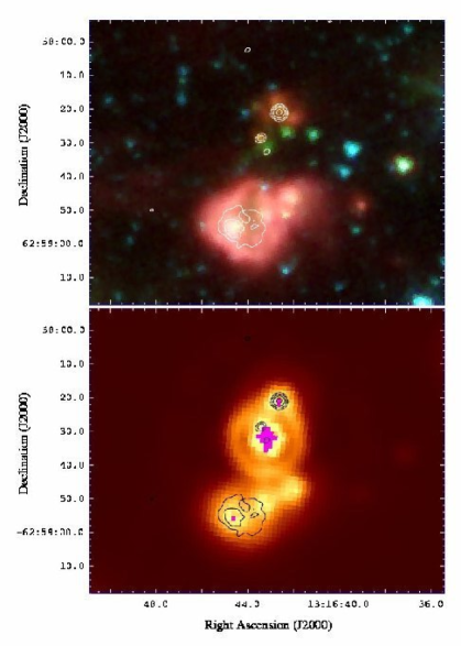
Figure 3: Comparison between the radio and IR images for G305.7984$-$00.2416. The white and black contours in each panel show 4.8 GHz data. Top panel: 3 color IRAC image using 8.0, 4.5, and 3.6 $\mu$m  data from Spitzer-GLIMPSE for red, green, and blue. Bottom panel: 24 $\mu$m MIPS image from Spitzer-MIPSGAL. Saturated pixels are shown in magenta.

In order to better determine the nature and evolutionary stage of these radio sources we present in the top panel of Figure 3 the three color MIR image, and in the bottom panel an image of the Spitzer-MIPSGAL 24 $\mu$m emission. Superimposed in these two images are contours of the 4.8 GHz emission. A comparison between the radio and MIR images shows that radio component A is associated with an extended MIR feature which is prominent at 8.0 $\mu$m, components B and C are associated with compact MIR objects GLIMPSE G305.7996$-$00.2438 and G305.7991$-$00.2447, respectively, and component D is associated with an extended envelope of diffuse emission most prominent at 8.0 $\mu$m, thought to arise from a photon dominated (or photo-dissociation) region (PDR, Heitsch et al., 2007).

The jet candidate corresponds to component A, which at 8.6 GHz exhibits a cometary-like structure with a head toward the north and a tail trailing to the south. Its radio continuum spectrum (see Figure 15) is well fitted by that of a uniform density H II region with an emission measure of $2.3\times 10^{6}$ pc cm^-6 and an angular size of 1.4″. The ionizing photon flux needed to excite this H II region is $9.6\times 10^{45}$ photons s^-1. We conclude that component A corresponds to a cometary UCH II excited by a B1-B0.5 ZAMS star. Methanol maser activity has been detected toward this field (Pestalozzi et al., 2005), although it was not possible to determine its precise location.

The radio continuum spectra of components B, C and D are shown in Figure 16. The spectra of source B shows that its flux density is rising with frequency, suggesting that it corresponds to an optically thick H II region. A fit with a uniform density H II region model gives an emission measure of $1.3\times 10^{8}$ pc cm^-6 and an angular size of 0.066″. For component C we derived an emission measure of $1.0\times 10^{6}$ pc cm^-6 and an angular size of 0.9″. The ionizing photon rate needed to excite this H II region is $N_{i}\sim 2\times 10^{45}$ s^-1, which can be provided by a B1 ZAMS star. For component D we derived an emission measure of $2.0\times 10^{5}$ pc cm^-6 and an angular size of 8.1″. The ionizing photon rate needed to excite this extended and diffuse H II region is $N_{i}\sim 3\times 10^{46}$ s^-1, which can be provided by a B0.5 ZAMS star.

The G305.7984$-$00.2416 region may be representative of what is likely to see within the maternities of high-mass stars: a cluster of young stars in different evolutionary stages. We find that the target radio source in the field is not a jet but an UC H II. The weakest radio source detected in the region (Component B) is particularly striking because, as shown in Fig. 3, it is associated with a green object in the three color Spitzer image, possibly indicating shock activity. Extended green objects (EGOs, Chambers et al., 2009; Cyganowski et al., 2008) are thought to probe shocked gas regions associated with HMYSOs through vibrational H₂ and CO bands. However, hydrogen Br$\alpha$ contribution cannot be ruled out (Qiu et al., 2011). Even though a consistent scale have been applied to make all three-color IRAC images presented in this work, precaution is needed in interpreting the images. The community has not adopted an standardized procedure to make these images, casting doubts on the physical significance of some of the “green fuzzies” (e.g. De Buizer & Vacca, 2010).

The position of Component B is consistent with the peak of the emission in the MSX band E (21.34 $\mu$m ) image (marked with a square in Fig. 2), and it also seems to be the brightest source in the 24 $\mu$m MIPS image (Fig. 3), despite the saturation of the central pixels. This evidence suggests that component B is actually the most embedded, and possibly the youngest, object in the region. Using the GLIMPSE flux densities and assuming that the MSX E band flux arises entirely from this source, the YSO spectral energy distribution (SED) model fitter of Robitaille et al. (2007) gives a total luminosity of $3.3\pm 0.9\times 10^{3}$ $L_{\sun}$, equivalent to that of a B2 ZAMS star. The ratio between the ionizing photon flux derived from the radio SED fitting ($N_{i}\sim 1.2\times 10^{45}$ s^-1) and that inferred from the total luminosity ($N_{\star}\sim 6.3\times 10^{44}$ s^-1) is 1.9, implying that this radio source is slightly under-luminous in radio. Given its characteristics, particularly the association to green fuzzy emission, we suggest that component B could represent the transition phase as an early B-type star grows onto an O-type star. The excess emission at 4.5 $\mu$m may arise from shocks produced in the infalling gas.

G317.4298$-$00.5612.– This jet candidate is associated with the RMS/MSX source G317.4298$-$00.5612 (also IRAS 14477$-$5947). The kinematical distance of the object is $15$ kpc, with no ambiguity ($v_{LSR}=27.4$ km s^-1 in the CS(2$\rightarrow$1) line, Bronfman et al., 1996) and assuming a flat rotation curve ($\Theta=220$ km s^-1). From the bolometric flux given by Mottram et al. (2011a) we estimate a total luminosity of $L\sim 3.2\times 10^{5}$ $L_{\sun}$, equivalent to that of a ZAMS star with an spectral type between O6 and O5.5. Water maser has been detected toward this source by Urquhart et al. (2009).

Figure 4 shows that there are two radio objects within the $80\arcsec\times 80\arcsec$ region: a compact component (labeled A), seen only at 4.8 and 8.6 GHz, and an extended component (labeled B) mainly seen at 1.2 and 2.4 GHz and completely resolved out at 8.6 GHz.

Component A corresponds to the jet candidate. At 1.4 and 2.4 GHz this object is immersed within the more extended component so we could not measure its flux densities. In the frequency range between 4.8 and 8.6 GHz, the flux density rises with frequency. Since the source is unresolved, from these data it is not possible to discern whether this object is a jet or an optically thick H II region. If an H II region, then a fit to the radio continuum spectrum with an uniform density model (see Fig. 15) indicates an emission measure of $1.9\times 10^{8}$ pc cm^-6 and an angular size of 0.27″. The rate of ionizing photons required to excite this region of ionized gas is $7.2\times 10^{47}$ s^-1, which can be provided by a O9.5 ZAMS star.

The radio continuum spectrum of component B (see Figure 16) suggests it corresponds to an extended optically thin H II region. A fit with a theoretical spectra of an homogeneous constant density H II region gives an emission measure of $3.5\times 10^{5}$ pc cm^-6 and an angular size of 7.6″. The rate of ionizing photons required to excite the H II region is $9.3\times 10^{47}$ s^-1, which can be provided by a O9.5 ZAMS star.

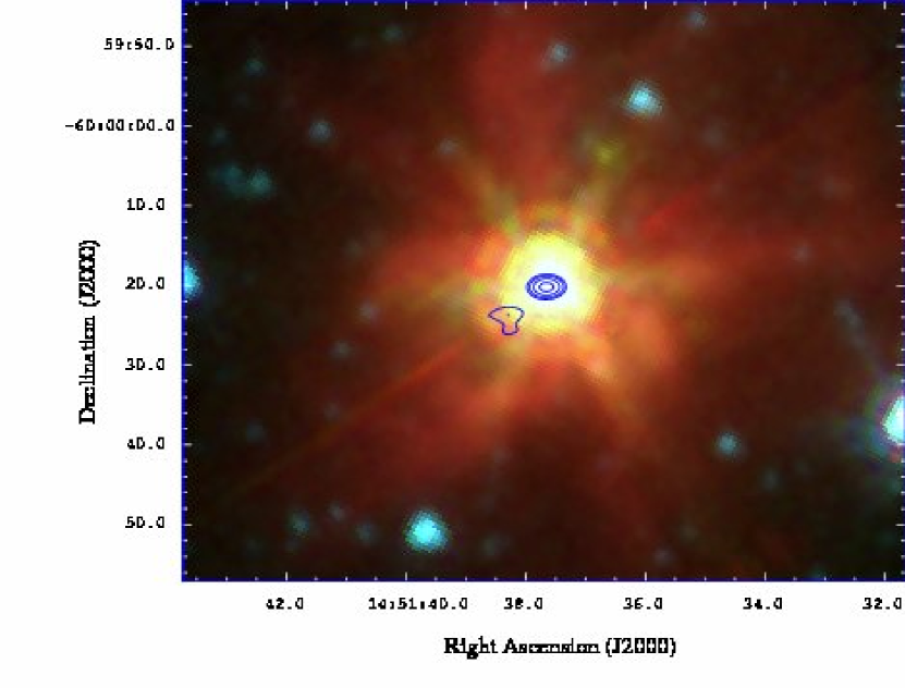
Figure 5: Comparison between mid-infrared and radio emission data detected toward G317.4298$-$00.5612. The color image correspond to a three color IRAC image using 8.0, 4.5, and 3.6 $\mu$m data from Spitzer-GLIMPSE for red, green, and blue. Blue contours show 4.8 GHz data.

Figure 5 shows the three color mid-infrared IRAC image toward this region. Component A is associated with a bright MIR source with colors similar to a PDR associated to an UCH II region.

The sum of the luminosities of the ZAMS stars exciting components A and B is $8\times 10^{4}$ $L_{\sun}$, about 4 times smaller than the bolometric luminosity of the whole region. This discrepancy may be solved if component A is not an H II region but an ionized jet, in which core the exciting source could have a larger luminosity than that implied from the observed radio flux density. Further observations are needed to confirm this interpretation.

G337.4032$-$00.4037.– This jet candidate is associated with the RMS source G337.4032$-$00.4037 (also IRAS 16351$-$4722). Figure 6 shows that there are two radio sources within the $80\arcsec\times 80\arcsec$ region: a bright compact component (labeled A) and a weak component, labeled B, located about 13″ southeast of component A. Component A, which corresponds to the jet candidate, is unresolved at all frequencies, whereas component B is resolved out at 4.8 and 8.6 GHz. Methanol maser activity has been associated to component A by Walsh et al. (1998), whereas no water maser was detected by Urquhart et al. (2009) at 0.25 Jy sigma level.

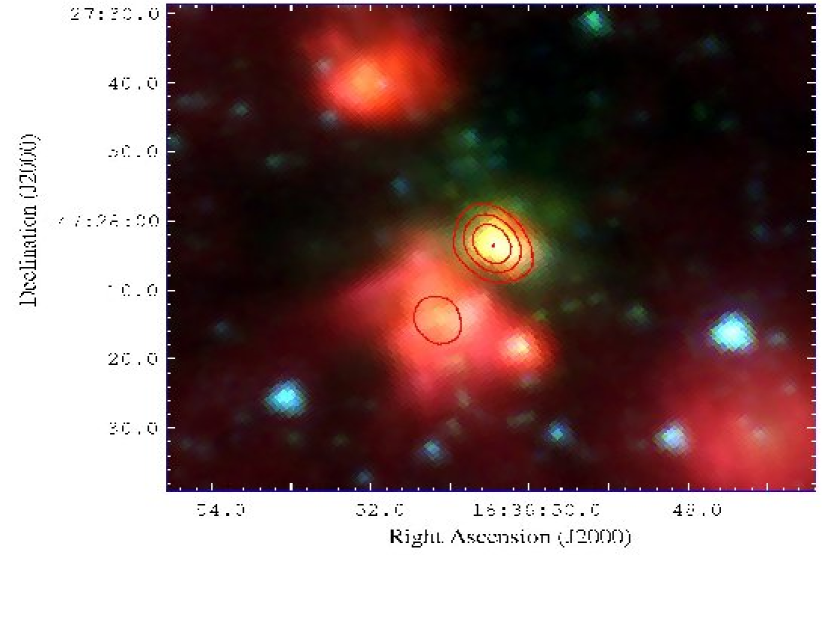
Figure 7: Three color MIR image toward G337.4032$-$00.4037 made using Spitzer-GLIMPSE images at 8.0, 4.5, and 3.6 $\mu$m for red, green, and blue, respectively. Red contours correspond to the 2.4 GHz radio data.

Figure 7 shows the three-color IRAC image of the MIR emission detected toward this region, and in red contours the 2.4 GHz data. This Figure shows that component A is associated with the central, bright, greenish-like object seen in the Spitzer image. Assuming that this star forming region is at a distance of 3.2 kpc (Faúndez et al., 2004), then from the bolometric flux reported by Mottram et al. (2011a, their component “B”), we obtain a bolometric luminosity of $2.7\times 10^{4}$ $L_{\sun}$, equivalent to that of B0 ZAMS star.

The radio continuum spectrum of component A (see Figure 15) shows that the flux density steadily increases with frequency. A power law fit gives an spectral index of $0.9\pm 0.15$, consistent with a pressure confined jet (Reynolds, 1986). Using equation (19) of Reynolds (1986), assuming typical values (e.g. Guzmán et al., 2010) of 45^∘ for the inclination, 0.2 rad for the jet aperture, a turnover frequency of 20 GHz and a wind velocity of 300 km s^-1, we obtain a mass loss rate of $\dot{M}\approx 2\times 10^{-5}\mbox{\,$M_{\sun}$}$ yr^-1.

Our interpretation of this source as a jet is supported by the association to a very high velocity molecular outflow. Figure 8 shows the CO $J=3\rightarrow 2$ emission detected toward G337.4032$-$00.4037 using the Atacama Pathfinder EXperiment (APEX). A description of the instrument and its performance is given by Güsten et al. (2006) and a detailed account of these observations can be found in Guzmán (2011). The presence of high-velocity gas is evident from Fig. 8, where the line emission can be detected in a $\sim 120$ km s^-1 range. The ambient gas velocity respect to the local standard of rest (LSR) is $-$40.7 km s^-1.

Radio continuum spectra similar to the one exhibited by this source have usually been interpreted as arising from hypercompact H II regions (HCH IIRs, Franco et al., 2000) with power-law dependence of the density with radius (e.g., Panagia & Felli, 1975; Avalos et al., 2006). For an spherical H II region in which the density follows $n_{e}\propto r^{-\beta}$, the flux density should exhibit a power-law dependence with frequency, $S_{\nu}\propto\nu^{\alpha}$, with $\alpha=(2\beta-3.2)/(\beta-0.5)$. There is no hint of an spectrum turn over at high frequencies, indicating that the emission does not reach optically thin conditions in the whole observed frequency range. Assuming ionization equilibrium, with $N_{\star}\sim 2.6\times 10^{47}$ s^-1(appropriate for a ZAMS star with $2.7\times 10^{4}$ $L_{\sun}$), and that the power-law index of the density profile is 2.5 (determined from the above relationship), the observed spectrum and source size can be well reproduced if the region has an inner radius of 0.0032 pc, an outer radius of 0.044 pc and an electron density of $3.6\times 10^{5}$ cm^-3 at the inner radius. We note, however, that the jet and the HCH IIR models have many free parameters, and that these solutions are not unique.

Figure 7 also shows that component B is associated with the bright, central part of an extended, diffuse MIR object, most prominent at 8.0 $\mu$m and likely to correspond to a PDR around an H II region. From the bolometric flux reported by Mottram et al. (2011a), we derive a bolometric luminosity for component B of 8.4$\times 10^{4}$ $L_{\sun}$. The flux density expected at 1.4 GHz from an optically thin H II region excited by a star with that luminosity is $\sim 0.5$ Jy, considerably larger than the measured 5 mJy. This implies, as our observations indicate, that the flux density is resolved out by the interferometer even at 1.4 GHz.

G345.0061$+$01.7944.– This jet candidate is associated with the RMS/MSX source G345.0061$+$01.7944 (also IRAS 16533$-$4009). Figure 9 shows that there are two radio objects within the $80\arcsec\times 80\arcsec$ region: a compact component (labeled B) and an extended source, labeled A, located about 22″ southwest of component B. Component B, which corresponds to the jet candidate, is unresolved at all frequencies whereas component A is partially resolved out at 4.8 GHz and highly resolved out at 8.6 GHz.

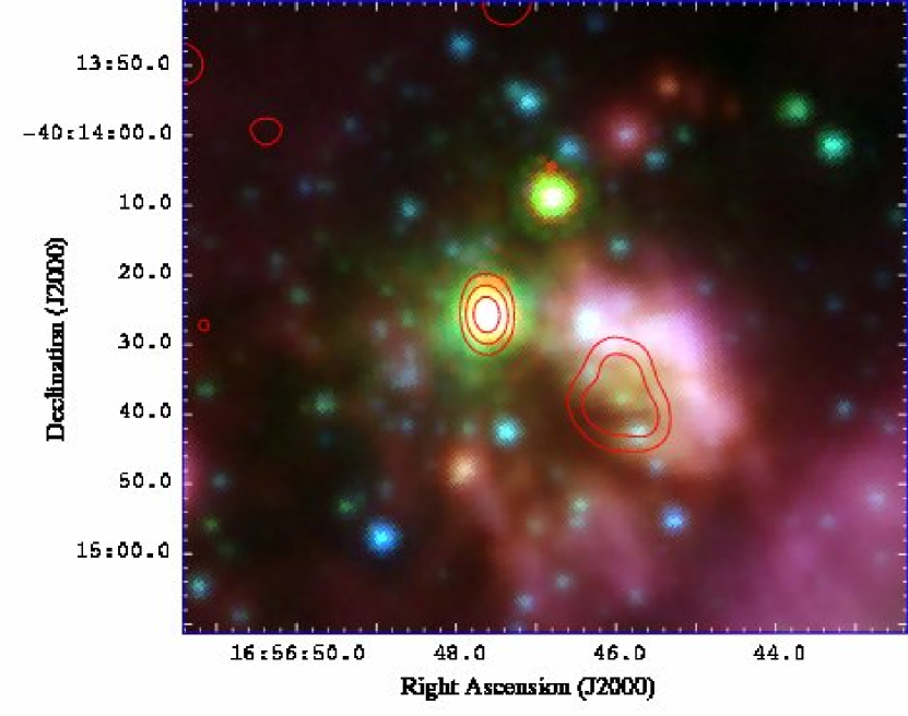
Figure 10: Three color Spitzer MIR image of G345.0061$+$01.7944, made using 8.0, 4.5, and 3.6 $\mu$m data from Spitzer-GLIMPSE for red, green, and blue, respectively. Superimposed red contours show the 2.4 GHz radio emission.

Figure 10 presents the three-color image of the MIR emission toward this region, together with red contours displaying the 2.4 GHz data. This Figure shows that component B is associated with a bright, compact MIR source with enhanced 4.5 $\mu$m band emission (green color) whereas component A is associated an extended source of diffuse emission most prominent at 8.0 $\mu$m. Methanol maser activity has been detected by Walsh et al. (1998) toward two positions: one associated to radio component B, and another located approximately 20″ to the northwest. These positions correspond to the position of the “green” sources seen in Fig. 10. Water maser activity has been detected in the field by Forster & Caswell (1999), but not directly associated to any radio or IR source.

The radio continuum spectrum of component B (see Figure 15) suggests it corresponds to an optically thick H II region. A fit with a theoretical spectra of an homogeneous constant density H II region, gives an emission measure of $4.6\times 10^{8}$ pc cm^-6 and an angular size of 0.73″. The rate of ionizing photons required to excite the H II region is $1.7\times 10^{47}$ s^-1, which can be provided by a B0 ZAMS star. Component B is associated with one of the three IR sources reported by Mottram et al. (2011a) within the region (their component “C”). From its bolometric flux, of $1.19\times 10^{-7}$ erg s^-1 cm^-2, and assuming it is at the near distance of 1.7 kpc, we derive that this IR source has a luminosity of $L_{bol}=1.1\times 10^{4}$ $L_{\sun}$ , equivalent to that of a B0.5 ZAMS star. The ionizing photon flux provided by such a star ($N_{\star}\approx 1.7\times 10^{46}$ s^-1) is about an order of magnitude smaller than that implied from the modeling of the radio spectra, being this source overluminous in radio rather than underluminous. We note however that there is considerable uncertainty in the determination of the bolometric flux: taking a value closer to the upper limit of the uncertainty range given by Mottram et al. ($1.94\times 10^{-7}$ erg s^-1 cm^-2), makes the radio and IR luminosities consistent with a photoionized region.

The radio continuum spectrum of component A indicates that it corresponds to an optically thin region of ionized gas. A fit with a theoretical spectra of an homogeneous constant density H II region, gives an emission measure of $5.0\times 10^{5}$ pc cm^-6 and an angular size of 8.0″. The rate of ionizing photons required to excite this H II region is $2.2\times 10^{46}$ s^-1, which can be provided by a B0.5 ZAMS star. Two of the three MIR sources identified by Mottram et al. (2011a, their components A and B) are associated with this radio component, but none is located at the peak of the radio emission.

G352.5173$-$00.1549.– This jet candidate, taken from the Walsh et al. (1998) survey, is associated with IRAS 17238$-$3516. Figure 11 shows that there are two radio sources within the $80\arcsec\times 80\arcsec$ region: a bright compact component (labeled A) detected at the four frequencies, and a weaker, presumably extended component (labeled B) only seen at 1.4 and 2.4 GHz and resolved out at the higher frequencies.

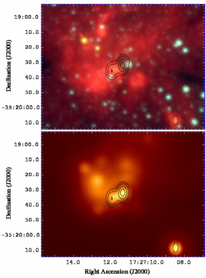
Figure 12: Mid-infrared images toward G352.5173$-$00.1549, with black contours corresponding to 1.4 GHz emission as seen in Fig. 11. Top Panel: 3 color IRAC image using 8.0, 4.5, and 3.6 $\mu$m data from Spitzer-GLIMPSE for red, green, and blue, respectively. The peak of the 1.4 GHz emission is consistent with the peak detected at higher frequencies, and to radio component A. The source seen $\sim 3$″ to the west is not embedded, and is unrelated with the radio emission. Radio component B appears to be related with the 8.0 $\mu$m diffuse emission seen at south-east from the peak. Bottom Panel: MIPS 24 $\mu$m emission. Component A is consistent with the peak at MIR wavelengths, and component B also shows MIR counterpart.

Component A, which corresponds to the jet candidate, can be well modeled by a homogeneous H II region with $T_{e}\sim 15000$ K, $\text{EM}\sim 2.8\times 10^{8}$ pc cm^-6 and an angular size of 0.42″ (Figure 15). The rate of ionizing photons required to excite this H II region is $3.2\times 10^{47}$ s^-1, which can be provided by a O9.5-B0 ZAMS star. The IRAC image shown in the upper panel of Figure 12 shows that component A is associated with a deeply embedded object seen conspicuously in MIPS at 24 $\mu$m (lower panel), but undetected in the GLIMPSE images, indicative of very high absorption. Note that the object located 3″ to the west of component A, seen at 4.5 and 3.6 $\mu$m (GLIMPSE 352.5170$-$00.1540), and in 2MASS bands (2MASS17271105$-$3519310), is a foreground object. Assuming that the emission detected in the IRAS bands (IRAS 17238$-$3516) corresponds to reprocessed emission from the exciting source of component A and that it is located at its kinematical (near) distance of 5.2 kpc, we derive a total luminosity of $\sim 10^{5}$ $L_{\sun}$, equivalent to that of an O7 ZAMS star. The ionizing photon rate expected from a star of that luminosity ($N_{\star}\sim 4.2\times 10^{48}$ s^-1) is about 13 times greater than that derived from the fit to the radio spectra, indicating that this source is intrinsically underluminous in radio. Water maser emission has been detected towards the central radio source (Forster & Caswell, 1999). Methanol maser activity has been detected toward this field (Pestalozzi et al., 2005), but its position is not well constrained by the observations.

We note that the flux at 8.64 GHz reported by Walsh et al. (1998) is $\sim 6$ times smaller than the flux measured by us at 8.6 GHz. Moderate flux variations in hypercompact H II regions have been detected (e.g. Galván-Madrid et al., 2008), but according to recent models, it is very unlikely to explain the large flux increment implied by our observations in a $\sim 10$ year basis (Galván-Madrid et al., 2011). Either the reason of the difference being observational or physical, we do not discuss it further in the present work.

Component B corresponds probably to a more developed H II region, which is consistent with the radio emission at the lower frequencies. Figure 12 shows that this source is associated with a faint 24 $\mu$m counterpart.

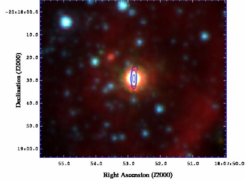
Figure 14: Comparison between the mid-infrared and radio emission detected toward G009.9937$-$00.0299. The color image correspond to a three color IRAC image using 8.0, 4.5, and 3.6 $\mu$m data from Spitzer-GLIMPSE for red, green, and blue. Blue contours show 4.8 GHz data.

G009.9937$-$00.0299.– This jet candidate, taken from Walsh et al. (1998), is associated with the MSX source G009.9983$-$00.0334 and with IRAS 18048$-$2019. It is the only radio source within the $80\arcsec\times 80\arcsec$ region shown in Fig. 13. Its radio continuum spectrum (see Fig. 15) can be well modeled with the theoretical spectra of an homogeneous constant density H II region. Assuming an electron temperature of $8000$ K, we derive an emission measure of $5.9\times 10^{5}$ pc cm^-6 and an angular size of 1.5″. The rate of ionizing photons required to excite the H II region is $7.9\times 10^{45}$ s^-1. Assuming that this object is located at 5 kpc — the near distance derived from the observed $v_{LSR}=49$ km s^-1 (Bronfman et al., 1996) — its total luminosity is 1.7$\times 10^{4}$ $L_{\sun}$ (Lackington, 2011), in between those of B0 and a B0.5 ZAMS stars, and for which $N_{\star}=7.9\times 10^{46}$ s^-1 (interpolated from Panagia 1973). The G009.9937$-$00.0299 object is then underluminous in radio by a factor of $\sim 10$. However, we do not see neither the spectral nor morphological features to characterize this radio source as a jet. Moreover, the three-color MIR image presented in Fig. 14 resembles that of G317.4298$-$00.5612, exhibiting a single central point source with color characteristic of photoionized gas. We conclude that this radio source corresponds to an UC H II region.

Walsh et al. (1998) reported methanol maser emission located approximately 45″ toward the southwest of the radio source and probably not directly related to it. Water maser activity has also been detected toward this source (Valdettaro et al., 2001).

5 DISCUSSION

5.1 Nature of the jet candidates

In this section we summarize the nature of 7 out of the 33 jet candidates listed in Table 1. We find that two candidates — G337.4032$-$00.4037 A and G345.4938$+$01.4677 — can be identified, from their radio continuum spectral characteristics, as ionized jets. Even though the angular resolution of the observations was insufficient to resolve the jet morphology, there is good evidence, such as the presence of collimated lobes of radio emission and energetic molecular outflows to consider these two objects as bona-fide collimated ionized winds.

To determine the physical parameters of the jet found toward G345.4938$+$01.4677 we assumed a pressure confined jet model (Guzmán et al., 2010). This model reproduces well the observed spectral indexes of G345.4938$+$01.4677 and G337.4032$-$00.4037 A. Despite of the fact that pressure has been rejected as the collimation mechanism of jets associated to low-mass stars (Cabrit, 2007), it is still a plausible mechanism in the high-mass case. Jets associated to HMYSOs are found near the center of high-mass star forming cores, which have enough density and temperature to confine a jet with the characteristics described above. Furthermore, ram pressure from infalling gas is also relevant in these cores. Infalling motions have been detected toward all cores associated with luminous HMYSOs with jets: G343.1262$-$00.0620, Garay et al. 2003; G345.4938$+$01.4677, Guzmán et al. 2011; and G337.4032$-$00.4037 A (Guzmán, 2011).

Three of the jet candidates, G317.4298$-$00.5612 A, G345.0061$+$01.7944 B, and G352.5173$-$00.1549 A, turned out to correspond to small ($D<0.03$ pc) regions of ionized gas with large emission measures (${\rm EM}>10^{8}$ pc cm^-6), and thus can be classified as hypercompact H II regions, according to the definition of Sewiło et al. (2011). HCH II regions are thought to trace the earliest stages of photoionized nebulae associated to single or binary high-mass star system system. To date, about a dozen of these regions are known (Hoare et al., 2007). Finally, the remaining two jet candidates observed, G009.9937$-$00.0299 and G305.7984$-$00.2416 A, correspond to UCH II regions (EM$>10^{6}$ pc cm^-6, size $<0.1$ pc). An important issue concerning the jet list candidates is whether the radio and FIR emission arise from the same object. At least in one case, G305.7984$-$00.2416 A, we found that the cataloged RMS radio source is not associated with the luminous object seen in IRAS bands, and that the much fainter component B is likely to be the youngest and more embedded source of this high-mass star maternity.

Considering the 7 jet candidates observed as part of this search, plus G343.1262$-$00.0620, which Garay et al. (2003) showed that corresponds to a collimated ionized jet, then there are 8 of the 33 jet candidates for which their nature have been determined. Of these, 37.5% corresponds to collimated ionized winds, 37.5% corresponds to HC H II regions and 25% corresponds to UCH II regions. Due to the homogeneity of the selection criteria used in building the jet candidate list (Table A) we expect the same proportion of objects in the whole list. Thus, we expect to find about 9 new ionized jets among the 25 candidates not yet observed.

5.2 Lifetime of jets in HMYSOs

Despite of the limited size of the sample of objects observed in this work, we can analyze the statistical incidence of jets from our observations and draw some conclusions about the lifetime of the jet phenomena in the formation process of high-mass stars. For the statistical analysis we will only consider the jet candidates chosen from the RMS survey. This selection allows us to make comparison with the results of a recently reported study of HMYSOs and compact H II regions (CH IIRs) identified in the RMS survey (Mottram et al., 2011b). In particular, they estimated that the lifetime of the CH IIR phase, for all range of luminosities, is $\sim 3\times 10^{5}$ yr. Of the 239 radio sources we initially considered from the entire RMS radio sample reported by Urquhart et al. (2007a), we find that 92 are located at angular distances smaller than 25″ from an IRAS point source with a luminosity $L>2\times 10^{4}$ $L_{\sun}$. We assume that these 92 sources form an unbiased sample of the CH II region population analyzed in Mottram et al. (2011b).

Of these 92 sources we find that 23 fulfill the two additional criteria required to be considered jet candidates: positive spectral index and radio underluminosity by a factor of at least 10. These are the objects with entry (1) in col. (10) of Table A. Since we can not disentangle the FIR luminosity from the jet candidates G301.1364$-$00.2249 A and B, and G317.8908$-$00.0578 A and B, we count them as if they were single objects. At the high luminosity of the sources we are sampling, completeness corrections of the RMS survey are small: about $0.8$ and $0.97$ for sources of $20,000$ and $30,000$ $L_{\sun}$, respectively, and essentially complete for more luminous HMYSOs (Mottram et al., 2011b).

We observed four jet candidates drawn from the RMS subsample and found that two of them are bona-fide jets (G337.4032$-$00.4037 A and G345.4938$+$01.4677). Using this detection rate, we then expect to find about 11 jets within the 23 candidates. The jet incidence in the population of CH II regions is therefore $\sim$11/92, which in combination with the CH II region average lifetime of $\sim 3\times 10^{5}$ yr (Mottram et al., 2011b) implies that the lifetime of the jet phase is roughly $4\times 10^{4}$ yr. This lifetime is comparable to the Kelvin-Helmholtz timescale of a HMYSO of $10^{4}$ $L_{\sun}$. Afterwards, the central protostar rapidly contracts onto the main sequence producing an HCH II region. This could explain why few jets are observed associated with HMYSOs.

Similarly, for the HCH II regions we derive lifetimes of the order of $4\times 10^{4}$ yr. Multiple radio sources in the field is an issue to consider within the RMS sample, but we found that all companion sources correspond to more diffuse and evolved H II regions.

5.3 The role of jets in high-mass star formation

Our systematic search have shown that jets occur in the formation process of high-mass stars, at least for HMYSOs with luminosities up to $1\times 10^{5}~{}\mbox{$L_{\sun}$}$. This result strongly suggests a disk-mediated accretion scenario for the formation of high-mass stars. The duration of the jet phase is short, $\sim 4\times 10^{4}$ yr, explaining why they are not commonly observed.

This age estimate allows us to assess the role of the collimated ionized jets in driving the larger scale molecular outflows observed toward HMYSOs. The mean mass loss rate estimated from the values of known jets (see Garay et al., 2003; Guzmán et al., 2011), is $\sim 5\times 10^{-6}\dot{\mbox{\,$M_{\sun}$}}$ yr^-1. Assuming that the jet velocities are $\sim 500\,\mbox{km s${}^{-1}$}$ (Anglada, 1996; Martí et al., 1998; Curiel et al., 2006; Rodríguez et al., 2008; Guzmán et al., 2010), then the momentum delivered by the jets is $\sim 100$ $M_{\sun}$ km s^-1. On the other hand, the mean masses and gas velocities of the massive molecular outflows reported by Beuther et al. (2002) are 25  $M_{\sun}$ and $28\,\mbox{km s${}^{-1}$}$, respectively, implying a mean momentum of $\sim 700$ $M_{\sun}$ km s^-1. Thus, even with the assumption that all of the jet momentum is transferred to the outflow (Richer et al., 2000), the jet momentum as estimated above falls short, by a factor of $\sim 7$, to drive the molecular outflow. This factor is similar to the one reported for G345.4938+01.4677 by Guzmán et al. (2011). There are at least two possible answers to explain this discrepancy: i) the jet is not entirely ionized, but their ionization fraction is about a 10% or below; ii) as appears in the radio images, the ejection of mass from the jet is episodic and highly discontinuous, most of the momentum being delivered during short bursts, and what we observe now correspond to a more “quiescent” phase of the jet.

6 SUMMARY

We are currently undertaking a systematic search of collimated jets towards high-mass young stellar objects with the goal of determining the pertinence of this phenomenon in the formation process of massive stars. In this paper we present the first results of multi-frequency radio continuum observations, made using ATCA, towards 6 HMYSOs candidates to harbor jets. Our main results and conclusions are summarized as follows.

1. We compiled a list of 33 HMYSOs likely to contain jets using a selection criteria based on their radio and infrared properties. The objects have large bolometric luminosities ($L>2\times 10^{4}~{}\mbox{$L_{\sun}$}$) and are underluminous at radio wavelengths compared to what is expected from the total luminosity.

2. We obtained radio continuum observations at 1.4, 2.4, 4.8, and 8.6 GHz using ATCA, towards six HMYSOs in the list. We find that one object corresponds to an ionized jet, three to hypercompact H II regions and two to ultracompact H II regions.

3. The jets discovered as part of this search, G337.4032$-$00.4037 and G345.4938$+$01.4677 – the latter reported and analyzed previously by Guzmán et al. (2010) – are associated with the two most luminous ($7\times 10^{4}$ and $1.0\times 10^{5}$ $L_{\sun}$) HMYSOs known to harbor this type of objects. This indicates that the phenomena of collimated ionized winds appears in the formation process of stars at least up to masses of $\sim 20$  $M_{\sun}$ and provides strong evidence for a disk-mediated accretion scenario for the formation of high-mass stars. From the rate of occurrence of jets in our sample, we estimate that the jet phase in high-mass protostars lasts for $\sim 4\times 10^{4}$ yr.

4. The estimated momentum that the observed ionized jets deliver during its main lifetime is about one tenth of the average momentum of the molecular outflows associated to HMYSOs. Whether this is a problem of the models or an actual inadequacy of the jets to explain the dynamics of molecular outflows remains to be resolved by future observations.

5. An important part of the observed candidates were found to correspond to hypercompact H II regions, thought to be an early phase in the development of the UCH IIR. These hypercompact regions probably appears right after the jet phase. We estimated their lifetime in a similar manner as done with the jets, obtaining also $\sim 40,000$ yr.

6. As part of this search, we performed observations toward 5 other HMYSOs that did not satisfied the criteria to be jet candidates. In the Appendix we present these observations and physical interpretation of the data.

Appendix A Other sources of interest

In this section we report the results of the observations on five radio sources, chosen from the Urquhart et al. (2007a) or Walsh et al. (1998) catalogs, but that do not fulfilled all the requirements to be considered jet candidates. These sources were selected in an early phase of our study, and they are most likely HMYSOs. These sources were observed together with the jet candidates, and the same reduction and calibration steps described in § 3 were applied.

Table 5 gives the phase tracking center, the on-source total integration times, the FWHM axes of the synthesized beam obtained at each frequency, and the deconvolved map noise levels for each observed field.

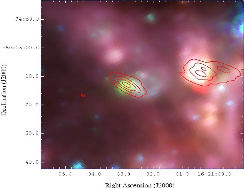
Figure 21: Three color IRAC image of G333.1306$-$00.4275 made using 8.0, 4.5, and 3.6 $\mu$m data from Spitzer-GLIMPSE for red, green, and blue, respectively. Intercalated contours of the 4.8 GHz data (Fig. 20) are shown in red.

Emission was detected toward four of the five objects: three of them correspond to ionized regions associated to a HMYSO, and one to an extragalactic source. Maps of the radio continuum emission at the frequencies of 1.4, 2.4, 4.8, and 8.6 GHz, in regions of 80″$\times 80$″ in size, are shown in Figures 17 through 20. The position of the target radio object, as reported in either catalog of is indicated in the maps with a cross. We also show in Figure 21 a mid-infrared 3 color image taken toward G333.1306$-$00.4275, that will be used to support its physical interpretation. Spectra of the four detected sources are shown in Fig. 22. The derived parameters, obtained from model fits to the spectra, are presented in Table 7. The columns display the same parameters as Table 4, described in § 4.

G263.7759$-$00.42813.– This radio source is associated with the RMS/MSX object G263.7759$-$00.4281 (also IRAS 08448$-$4343), which is known to be associated with an H₂O maser (Urquhart et al., 2009) and a H₂ bipolar flow (Giannini et al., 2005). The luminosity derived from the IRAS bands and assuming this source is located at a distance of 1.6 kpc (Urquhart et al., 2007b), is $\sim 3\times 10^{3}$ $L_{\sun}$, therefore failing our luminosity selection criterion. It is the only radio source within the $80\arcsec\times 80\arcsec$ region shown in Fig. 17. Its radio continuum spectrum (see Figure 22) can be well modeled with the theoretical spectra of an homogeneous constant density H II region. Assuming an electron temperature of $8000$ K, we derive an emission measure of $4.1\times 10^{6}$ pc cm^-6 and an angular size of 0.53″. The rate of ionizing photons required to excite the H II region is $7.0\times 10^{44}$ s^-1.

Using MSX, IRAS and TIMMI2 data, Mottram et al. (2011a) derived a bolometric flux of $F_{\rm bol}\approx 5.77\times 10^{-8}$ erg cm^-2 s^-1. At a distance of 1.6 kpc, we derive a bolometric luminosity of $L\sim 4.6\times 10^{3}$ $L_{\sun}$, equivalent to that of B1-B2 zero-age main sequence (ZAMS) star. The ionizing flux from such a star is $1.4\times 10^{45}$ s^-1 (interpolated from Panagia, 1973), similar to that required to excite the region of ionized gas. We conclude that this radio object corresponds to a small (0.004 pc in diameter), optically thin H II region excited by a single B1-B2 ZAMS star.

G268.6162$-$00.7389.– This radio source is associated with the RMS/MSX source G268.6162$-$00.7389 (also IRAS 09014$-$4736). It is the only radio source within the $80\arcsec\times 80\arcsec$ region shown in Fig. 18. No water masers were detected toward this source by Urquhart et al. (2009) at the 0.25 Jy sigma level. The luminosity derived from the IRAS bands and assuming this source is located at a distance of 1.7 kpc (Beck et al., 1991), is $\sim 5\times 10^{3}$$L_{\sun}$, therefore failing our luminosity selection criterion. The radio source is unresolved and its radio continuum spectrum (see Figure 22) is well fitted by that of a uniform density H II region with an emission measure of $7.0\times 10^{6}$ pc cm^-6, temperature of $15000$ K and an angular size of 0.84″. The ionizing photon flux needed to excite the H II region is $3.4\times 10^{45}$ photons s^-1.

Mottram et al. (2011a) reported for this object a bolometric flux of $7.1\times 10^{-11}$ W m^-2. At a distance of 1.7 kpc, the implied bolometric luminosity is $6.4\times 10^{3}$ $L_{\sun}$, equivalent to that of a ZAMS star with a spectral type between B0.5 and B1. The ionizing flux from such a star is $3.4\times 10^{45}$ s^-1 (interpolated from Panagia, 1973), equal to that required to excite the region of ionized gas. We conclude that this radio object corresponds to a small (0.007 pc in diameter), optically thin H II region excited by a single B0.5-B1 ZAMS star.

G327.1307+00.5259.– This radio source is in the field of the RMS source MSX-G327.1192$+$00.5103, although it is located at an angular distance of $\sim 1$′ to the north of the peak MSX emission and the closest IRAS point source (IRAS 15437$-$5343). No infrared counterpart has been detected at MIR wavelengths, neither in Spitzer (GLIMPSE or MIPSGAL) nor MSX, which makes it unlikely that this object corresponds to an embedded HMYSO.

It is the only radio source detected within the $80\arcsec\times 80\arcsec$ region shown in Fig. 19. Its radio continuum spectrum (see Figure 22) shows a decrease in the flux density at the higher frequencies. Being unresolved at all wavebands, the drop is not produced by the resolving power of the interferometer. We suggest that the radio emission from this source has a non-thermal origin. From the available evidence, we further suggest that this is an extragalactic source, possible a radio-loud galaxy. Figure 22 shows that the spectrum can be well fitted with a simple model of a gigahertz peaked galaxy (Snellen et al., 1998), the spectral indeces in the optically thick and thin regimes being 0.91 and $-$0.69, respectively. The lack of infrared emission could be explained by the source being intrinsically faint at these wavelengths compared to the radio emission, and/or due to absorption in the Galactic plane. Similar objects without MIR counterpart had already been detected in extragalactic surveys (Norris et al., 2006; Huynh et al., 2010).

G333.1306$-$00.4275.– This radio object was selected from the Urquhart et al. catalog due to its steep spectral index ($\gtrsim$ 1) between 4.8 and 8.6 GHz. It is located $\sim 25$″ east of the closest MSX source G333.1306$-$00.4275 (also IRAS 16172$-$5028), therefore failing our selection criteria. There are two radio sources within the $80\arcsec\times 80\arcsec$ region shown in Fig. 20: a compact central component (the target object; labeled B) and a complex, extended component, labeled A, associated with the RMS source.

The radio continuum spectrum of component B (see Figure 22) is well fitted with a power-law spectrum with a spectral index of $\sim 1$, similar to those of HC H II region (Franco et al., 2000). The bolometric flux is 15.4$\times 10^{-8}$ erg s^-1 cm^-2 (Mottram et al., 2011a), which at a distance of 3.5 kpc (Faúndez et al., 2004) implies that its total bolometric luminosity is $5.9\times 10^{4}$ $L_{\sun}$.

Figure 21 shows a three-color image of the MIR emission towards G333.1306$-$00.4275 made using the 3.6, 4.5, and 8.0 $\mu$m data obtained from the Spitzer/GLIMPSE survey, and superimposed in red contours the radio emission detected in 4.8 GHz. This figure clearly shows that component B is associated with a green extended object, thought to be related to regions of shocked gas. Component A is associated with a bright, extended MIR source, specially bright at 8.0 $\mu$m, associated with PAH emission in a PDR. The radio spectrum is flat (Fig. 22) and probably correspond to a more evolved H II region.

G345.3768+01.3926.– This source was chosen from the catalog of Walsh et al. (1998). It is located more than 1′ away from the nearest IRAS source (IRAS 16561$-$4006). Walsh et al. reported a peak flux of 5 mJy beam^-1 at 8.64 GHz and a flux density of 12.3 mJy. No sources were detected towards the radio position in GLIMPSE or MSX, which makes this object an unlikely YSO candidate. We do not detect emission towards this radio object in any of the four frequencies at the $\sim 0.1$ mJy beam^-1 level, indicating that this is a highly variable radio source. We propose an extragalactic origin. Such extreme variability in radio-loud galaxies is rare, but has been observed (e.g., Barvainis et al., 2005).

Table 1: Jet candidates

Source Name	$\alpha$	$\delta$	F${}_{\nu\text{-low}}$	F8.6GHz	S.I.	D	IRAS	LIRAS	Ref.
	(J2000)	(J2000)	(mJy)	(mJy)		(kpc)		($10^{4}$ $L_{\sun}$)
G240.3160$+$00.0714	07h44m52$\fs$04	$-$24°07′42$\farcs$4	$<$18	12.4	u	7.3	07427$-$2400	7.7	(2)
G274.0649$-$01.1460	09 24 42.13	$-$52 02 00.8	28.9	36.1	0.44	6.9	09230$-$5148	80.	(1)
G289.9446$-$00.8909	11 01 09.00	$-$60 56 56.3	$<0.7$	12.4	$\geq 2$	10.3	10591$-$6040	21.5	(1)
G293.9633$-$00.9776	11 32 36.14	$-$62 28 08.3	24.8	28.9	0.3	11.1	11303$-$6211	10.1	(1)
G298.2234$-$00.3393	12 10 01.16	$-$62 49 53.9	1350.	2200.	0.96	11.3	12073$-$6233	463.	(1)
G300.9674$+$01.1499	12 34 53.23	$-$61 39 40.1	102.	138.	0.6	4.4	12320$-$6122	22.6	(1)
G301.1364$-$00.2249A	12 35 35.13	$-$63 02 31.7	83.8	228.	2.	4.4	12326$-$6245	32.	(1)
G301.1364$-$00.2249B	12 35 35.19	$-$63 02 24.0	126.	179.	0.68	4.4	12326$-$6245	32.	(1)
G305.7984$-$00.2416	13 16 42.62	$-$62 58 21.2	$<$10	5.	u	3.	13134$-$6242	3.4	(2)
G308.9176$+$00.1231	13 43 01.72	$-$62 08 56.1	247.	374.	0.81	5.3	13395$-$6153	25.6	(1)
G309.9196$+$00.4791	13 50 41.89	$-$61 35 11.5	377.	384.	0.072	5.4	13471$-$6120	27.	(2)
G311.1359$-$00.2372	14 02 09.93	$-$61 58 37.9	3.0	3.5	0.3	14.3	13585$-$6144	11.7	(1)
G317.4298$-$00.5612	14 51 37.60	$-$60 00 19.4	6.6	8.2	0.42	15.0	14477$-$5947	63.4	(1)
G317.8908$-$00.0578A	14 53 06.19	$-$59 20 56.7	$<0.7$	3.6	$\geq 2$	15.1	14492$-$5908	19.7	(1)
G326.4477$-$00.7485	15 49 18.67	$-$55 16 52.5	4.7	5.9	0.39	4.3	15454$-$5507	2.1	(1)
G328.5759$-$00.5285B	15 59 38.15	$-$53 45 27.9	326	381	0.27	11.4	15557$-$5337	368.	(1)
G331.4181$-$00.3546	16 12 50.24	$-$51 43 28.6	80.7	83.9	0.07	4.1	16090$-$5135	5.7	(1)
G333.0162$+$00.7615	16 15 18.70	$-$49 48 52.8	46.9	88.8	1.2	3.3	16115$-$4941	6.1	(1)
G336.9842$-$00.1835	16 36 12.42	$-$47 37 58.0	18.	34.3	1.3	10.8	16325$-$4731	38.	(1)
G337.4032$-$00.4037	16 38 50.45	$-$47 28 02.7	90.3	130.	0.71	3.2	16351$-$4722	10.6	(1)
G337.7051$-$00.0575	16 38 29.63	$-$47 00 35.3	76.3	171.	1.6	12.2	16348$-$4654	53.1	(1)
G337.8442$-$00.3748	16 40 26.67	$-$47 07 13.1	11.1	24.4	1.5	3.1	16367$-$4701	3.9	(1)
G340.0708$+$00.9267	16 43 15.69	$-$44 35 16.0	48.8	93.8	1.1	4.9	16396$-$4429	7.2	(1)
G340.2768$-$00.2104	16 48 53.30	$-$45 10 22.3	$<1$	4.7	$\geq 2$	3.6	16452$-$4504	8.0	(1)
G343.1262$-$00.0620	16 58 17.21	$-$42 52 07.1	$<$7.3	4.62	u	2.9	16547$-$4247	6.3	(2)
G345.0061$+$01.7944	16 56 47.59	$-$40 14 25.8	127.	209.	0.98	1.7	16533$-$4009	5.4	(1)
G345.4938$+$01.4677	16 59 41.61	$-$40 03 43.4	4.8	12.5	1.9	1.7	16562$-$3959	7.0	(1)
G352.5173$-$00.1549	17 27 11.32	$-$35 19 32.8	$<$14	7.5	u	5.6	17238$-$3516	9.9	(2)
G000.3138$-$00.2000	17 47 09.66	$-$28 46 27.7	8.3	14.5	2.2	8.0	17439$-$2845	48.	(2)
G009.9937$-$00.0299	18 07 52.84	$-$20 18 29.3	$<$10	2.32	u	5.0	18048$-$2019	2.1	(2)
G010.8403$-$02.5913	18 19 12.10	$-$20 47 30.7	$<$21	4.8	u	1.9	18162$-$2048	2.5	(2)
G024.4673$+$00.4910	18 34 08.12	$-$07 18 18.2	$<$28	13	u	5.9	18314$-$0720	44.	(2)
G025.6469$+$01.0534	18 34 20.91	$-$05 59 39.3	$<$7	1.4	u	3.1	18316$-$0602	2.9	(2)

References. — (1):Urquhart et al. (2007a), (2): Walsh et al. (1998).

Table 2: Observational parameters of the observed jet candidates

				Synthesized Beam					Noise (mJy beam-1)
Source	Phase Tracking Center		Time	1.4GHz	2.4GHz	4.8GHz	8.6GHz		1.4GHz	2.4GHz	4.8GHz	8.6GHz
	$\alpha$(J2000)	$\delta$(J2000)	(mins.)	(″)	(″)	(″)	(″)		(mJy)	(mJy)	(mJy)	(mJy)
G305.7984$-$00.2416	13 16 42.62	$-$62 58 21.2	090	$\phantom{0}6.6\times 6.3$	$\phantom{0}4.4\times 3.9$	$2.2\times 1.7$	$1.1\times 0.9$		0.2	0.2	0.07	0.08
G317.4298$-$00.5612	14 51 37.60	$-$60 00 19.8	110	$\phantom{0}9.9\times 5.4$	$\phantom{0}6.8\times 3.8$	$2.8\times 1.7$	$2.1\times 1.1$		0.2	0.2	0.1	0.08
G337.4032$-$00.4037	16 38 50.45	$-$47 28 02.7	240	$\phantom{0}8.1\times 6.0$	$\phantom{0}5.4\times 3.9$	$2.2\times 1.7$	$1.1\times 0.9$		0.4	0.2	0.08	0.09
G345.0061$+$01.7944	16 56 47.59	$-$40 14 25.8	180	$\phantom{0}8.7\times 5.9$	$\phantom{0}5.6\times 4.0$	$2.6\times 2.0$	$1.4\times 1.0$		0.3	0.3	0.1	0.2
G352.5173$-$00.1549	17 27 11.32	$-$35 19 32.8	120	$10.1\times 5.6$	$\phantom{0}6.4\times 3.7$	$3.1\times 2.0$	$1.7\times 1.0$		0.2	0.2	0.2	0.1
G009.9937$-$00.0299	18 07 52.84	$-$20 18 29.3	110	$20.1\times 5.1$	$12.5\times 3.0$	$5.9\times 1.7$	$3.2\times 0.9$		0.2	0.1	0.06	0.05

Table 3: Observed parameters of radio sources

	Coordinates			Flux density					Deconvolved Sizes
	R.A.	Dec.		1.4 GHz	2.4 GHz	4.8 GHz	8.6 GHz		1.4 GHz	2.4 GHz	4.8 GHz	8.6 GHz
Source	(J2000)	(J2000)		(mJy)	(mJy)	(mJy)	(mJy)		(″)	(″)	(″)	(″)
Jet candidates
G305.7984$-$00.2416 A	13h16m42$\fs$63	$-$62°58′20$\farcs$9		10.4	11.2	11.2	9.3		U	1.4	1.4	1.4
G317.4298$-$00.5612 A	14 51 37.63	$-$60 00 20.2		$\cdots$	$\cdots$	11.0	19.7		$\cdots$	$\cdots$	U	0.36
G337.4032$-$00.4037 A	16 38 50.47	$-$47 28 03.1		27.8	56.7	110.3	139.5		1.6	1.2	0.5	0.8
G345.0061$+$01.7944 B	16 59 37.76	$-$40 12 03.8		12.2	44.4	152.5	271.8		1.3	U	0.7	0.7
G352.5173$-$00.1549 A	17 27 11.32	$-$35 19 32.2		4.4	14.1	40.5	66.0		U	U	0.9	0.4
G009.9937$-$00.0299	18 07 52.82	$-$20 18 28.9		3.4	3.5	3.2	2.3		U	U	U	U
Additional sources detected in the fields
G305.7984$-$00.2416 B	13 16 43.23	$-$62 58 32.9		$\cdots$	$\cdots$	0.7	1.0		$\cdots$	$\cdots$	U	U
G305.7984$-$00.2416 C	13 16 43.41	$-$62 58 28.7		1.2	2.2	1.8	2.0		U	U	U	0.9
G305.7984$-$00.2416 D	13 16 44.50	$-$62 58 54.7		32.6	27.6	24.2	35.0		8.0	10	10	10
G317.4298$-$00.5612 B	14 51 38.46	$-$60 00 24.3		41.6	48.9	5.7	$\cdots$		7.9	7.1	7	$\cdots$
G337.4032$-$00.4037 B	16 38 51.13	$-$47 28 14.8		5.0	5.1	6.5	4.7		U	U	2.6	$\sim 2$
G345.0061$+$01.7944 A	16 56 45.97	$-$40 14 38.1		91.4	99.1	83.0	72		7.1	8.1	$\sim 8$	$\sim 8$
G352.5173$-$00.1549 B	17 27 11.91	$-$35 19 35.5		2.8	1.6	$\cdots$	$\cdots$		U	U	$\cdots$	$\cdots$

Table 4: Derived parameters of the radio sources

	Dist.	Te	EM	$\theta$	Ni	D	$\langle n_{e}\rangle$	Type
Source	(kpc)	($10^{4}$K)	(pc cm-6)	(″)	($10^{45}$s-1)	(pc)	(cm-3)
Jet candidates
G305.7984$-$00.2416 A	3.0	0.8	$2.30\times 10^{6}$	1.40	$9.56$	0.020	$1.1\times 10^{4}$	UC H II
G317.4298$-$00.5612 A	15.	0.8	$1.90\times 10^{8}$	0.27	$718$	0.020	$9.8\times 10^{4}$	HC H II
G337.4032$-$00.4037 A	3.2	0.8	$>2\times 10^{8}$	$<0.64$	$\cdots$	$<0.01$	$>1.5\times 10^{5}$	jet
G345.0061$+$01.7944 B	1.7	1.5	$4.60\times 10^{8}$	0.73	$170$	0.006	$2.8\times 10^{5}$	HC H II
G352.5173$-$00.1549 A	5.2	1.5	$2.80\times 10^{8}$	0.42	$318$	0.011	$1.0\times 10^{5}$	HC H II
G009.9937$-$00.0299	5.0	0.8	$5.94\times 10^{5}$	1.49	$7.89$	0.036	$4.1\times 10^{3}$	UC H II
Additional sources detected in the fields
G305.7984$-$00.2416 B	3.0	1.0	$1.3\times 10^{8}$	0.066	$1.23$	0.001	$3.67\times 10^{5}$	HC H II
G305.7984$-$00.2416 C	3.0	0.8	$1.0\times 10^{6}$	0.901	$1.74$	0.013	$8.74\times 10^{3}$	UC H II
G305.7984$-$00.2416 D	3.0	0.8	$2.0\times 10^{5}$	8.027	$27.6$	0.117	$1.31\times 10^{3}$	C H II
G317.4298$-$00.5612 B	15.0	0.8	$3.5\times 10^{5}$	7.030	$926.$	0.511	$8.30\times 10^{2}$	C H II
G337.4032$-$00.4037 B	3.2	0.8	$3.0\times 10^{5}$	2.657	$5.16$	0.041	$2.70\times 10^{3}$	UC H II
G345.0061$+$01.7944 A	1.7	0.8	$5.0\times 10^{5}$	8.027	$22.2$	0.066	$2.75\times 10^{3}$	UC H II
G352.5173$-$00.1549 B	5.2	0.8	$5.0\times 10^{5}$	1.329	$5.68$	0.033	$3.86\times 10^{3}$	UC H II

Table 5: Observational parameters of other sources of interest

				Synthesized Beam					Noise (mJy beam-1)
Source	Phase Tracking Center		Time	1.4GHz	2.4GHz	4.8GHz	8.6GHz		1.4GHz	2.4GHz	4.8GHz	8.6GHz
	$\alpha$(J2000)	$\delta$(J2000)	(mins.)	(″)	(″)	(″)	(″)		(mJy)	(mJy)	(mJy)	(mJy)
G263.7759$-$00.4281	08h46m34$\fs$85	$-$43°54′29$\farcs$8	060	$14.0\times 5.0$	$\phantom{0}9.0\times 3.3$	$4.6\times 1.9$	$2.5\times 1.0$		0.1	0.1	0.07	0.08
G268.6162$-$00.7389	09 03 09.51	$-$47 48 27.3	060	$13.0\times 4.4$	$\phantom{0}9.2\times 3.2$	$4.7\times 1.9$	$2.6\times 1.0$		0.3	0.1	0.06	0.07
G327.1307+00.5259	15 47 32.47	$-$53 51 30.9	180	$\phantom{0}7.2\times 6.3$	$\phantom{0}4.9\times 4.2$	$2.3\times 1.9$	$1.2\times 1.0$		0.2	0.1	0.09	0.07
G333.1306$-$00.4275	16 21 02.95	$-$50 35 12.3	060	$12.1\times 4.4$	$\phantom{0}7.0\times 2.7$	$4.9\times 1.5$	$2.8\times 0.8$		3.1	1.8	2.1	3.4
G345.3768$+$01.3926	16 59 37.75	$-$40 12 03.5	170	$\phantom{0}9.0\times 5.6$	$\phantom{0}5.7\times 3.7$	$2.6\times 2.0$	$1.4\times 1.0$		0.1	0.1	0.08	0.08

Table 6: Observed parameters of other radio sources of interest

	Coordinates			Flux density					Deconvolved Sizes
	R.A.	Dec.		1.4 GHz	2.4 GHz	4.8 GHz	8.6 GHz		1.4 GHz	2.4 GHz	4.8 GHz	8.6 GHz
Source	(J2000)	(J2000)		(mJy)	(mJy)	(mJy)	(mJy)		(″)	(″)	(″)	(″)
G263.7759$-$00.4281	08 46 34.848	$-$43 54 30.27		2.0	3.2	2.7	2.4		U	U	U	U
G268.6162$-$00.7389	09 03 09.499	$-$47 48 27.66		8.6	9.1	10.0	9.2		U	1.6	1.1	0.7
G327.1307+00.5259	15 47 32.472	$-$53 51 31.58		20.0	22.5	19.5	13.3		U	0.9	U	0.36
G333.1306$-$00.4275 B	16 21 02.921	$-$50 35 12.92		186	604	1100	2000		U	U	5.9	3.3
G345.3768+01.3926	$\cdots$			$\cdots$					$\cdots$
Additional sources detected in the fields
G333.1306$-$00.4275 A	16 21 00.30	$-$50 35 08.30		1100	1589	1348	1664		$\sim 25$

Table 7: Derived parameters of the radio sources

	Dist.	Te	EM	$\theta$	Ni	D	$\langle n_{e}\rangle$	Type
Source	(kpc)	($10^{4}$K)	(pc cm-6)	(″)	($10^{45}$s-1)	(pc)	(cm-3)
Other sources of interest
G263.7759$-$00.4281	1.6	0.8	$4.05\times 10^{6}$	0.53	$0.697$	0.004	$3.2\times 10^{4}$	UC H II
G268.6162$-$00.7389	1.7	1.5	$7.00\times 10^{6}$	0.84	$3.40$	0.007	$1.9\times 10^{4}$	UC H II
G333.1306$-$00.4275 B	3.5	1.5	$>2\times 10^{8}$	$<2.5$	$\cdots$	$<0.042$	$>7.1\times 10^{4}$	HC H II
Additional sources detected in the fields
G333.1306$-$00.4275 A	3.5	0.8	$1.0\times 10^{6}$	24.998	$1820$	0.424	$1.54\times 10^{3}$	C H II

Figure 1: Radio luminosity at 8.6 GHz versus L_IRAS luminosity (Eq. 1) for all jet candidates in Table A. The continuous line indicates the expected radio luminosity of an optically thin H II region ionized by a ZAMS star (Panagia, 1973). The dashed line illustrates graphically the third selection criterion. Sources observed as part of the jet search described in this work are encircled. Squares mark objects G343.1262$-$00.0620 (also IRAS 16547$-$4247), G345.4938$+$01.4677 (IRAS 16562$-$3959), and G337.4032$-$00.4037.

Figure 2: ATCA maps of the radio continuum emission toward G305.7984$-$00.2416. The cross marks the position of the radio source reported by Walsh et al. (1998). Beams are shown in the lower left corner of each panel. Top left: 1.4 GHz map. The squares mark the peak position of two MSX 21 $\mu$m sources in the field. Top right: 2.4 GHz map. Bottom left: 4.8 GHz map. Labeled are the four radio sources detected in this field. Bottom right: 8.6 GHz map. Contour levels are $-$5, 5, 8, 13, 20, 30, 46, and 70 times 0.16 mJy beam^-1 for the 1.4 and 2.4 GHz maps, and 0.07 mJy beam^-1 for the 4.8 and 8.6 GHz maps.

Figure 4: ATCA maps of the radio continuum emission toward G317.4298$-$00.5612. The cross marks the position of the radio source reported by Urquhart et al. (2007a). Beams are shown in the lower left corner of each panel. Top left: 1.4 GHz map. The square marks the peak position of the MSX source detected at 21 $\mu$m. Top right: 2.4 GHz map. Bottom left: 4.8 GHz map. Labeled are the two radio sources detected in this field. Bottom right: 8.6 GHz map. Contour levels are $-$5, 5, 7, 9, 13, 19, 27, 40 times 0.5, 0.5, 0.2, and 0.4 mJy beam^-1 for the 1.4, 2.4, 4.8 and 8.6 GHz images, respectively.

Figure 6: ATCA maps of the radio continuum emission toward G337.4032$-$00.4037. The cross marks the position of the radio source reported by Urquhart et al. (2007a). Beams are shown in the lower left corner of each panel. Top left: 1.4 GHz map. The squares show the peak position of the three MSX 21 $\mu$m sources in the field. The star marks the position of the methanol masers detected by Walsh et al. (1998). Top right: 2.4 GHz map. Labeled are the two radio sources detected in the field. Bottom left: 4.8 GHz map. Bottom right: 8.6 GHz map. Contour levels are $-5$, 5, 14, 28, 50, 81, 129, and 200 times 0.25 mJy beam^-1 for the 1.4 and 2.4 GHz images, and $-5$, 5, 29, 65, 118, 199, 319, and 500 times 0.15 mJy beam^-1 for the 4.8 and 8.6 GHz images.

Figure 8: CO(3$\rightarrow$2) spectrum observed toward G337.4032$-$00.4037 using APEX. The v_LSR of the ambient gas associated to the source is $-$40.7 km s^-1. High-velocity molecular gas emission is detected between $-$85 and 41 km s^-1, spanning 126 km s^-1.

Figure 9: ATCA maps of the radio continuum emission towards G345.0061$+$01.7944. The cross marks the position of the radio source reported by Urquhart et al. (2007a). Beams are shown in the lower left corner of each panel. Top left: 1.4 GHz map. The square marks the peak position of the MSX source detected at 21 $\mu$m, the triangle the position of the H₂O maser reported by Forster & Caswell (1999), and the stars the position of methanol masers detected by Walsh et al. (1998). Top right: 2.4 GHz map. Bottom left: 4.8 GHz map. Labeled are the two radio components detected in the field. Bottom right: 8.6 GHz map. Contour levels are $-$5, 5, 11, 19, 31, 50, 78, 120 times 0.4 mJy beam^-1 for the 1.4 and 2.4 GHz images and $-5$, 5, 14, 28, 50, 81, 129, 200 times 0.4 mJy beam^-1 for the 2.4 and 8.6 GHz images.

Figure 11: ATCA maps of the radio continuum emission towards G352.5173$-$00.1549. Beams are shown in the lower left corner of each panel. The cross marks the position of the radio source reported by Walsh et al. (1998). Top left: 1.4 GHz map. Contour levels are $-$5, 5, 8, 13, and 18 $\times$ 0.20 mJy beam^-1. Labeled are the two radio components detected in the field. Squares mark the position of MSX sources. The triangle marks the position of the H₂O maser detected by Forster & Caswell (1999). Top right: 2.4 GHz map. Contour levels are $-$5, 5, 8, 13, 18, 26, 36, and 50 $\times$ 0.20 mJy beam^-1. Bottom left: 4.8 GHz map. Contour levels are $-$5, 5, 8, 13, 18, 26, 36, and 50 $\times$ 0.60 mJy beam^-1. Bottom right: 8.6 GHz map. Contour levels are $-$3, 3, 9, 18, 29, 44, 64, and 90 $\times$ 0.60 mJy beam^-1.

Figure 13: ATCA maps of the radio continuum emission toward G009.9937$-$00.0299. The cross marks the position of the radio source reported by Walsh et al. (1998). Beams are shown in the lower left corner of each panel. Top left: 1.4 GHz map. The square marks the peak position of the associated MSX source G009.9983$-$00.0334 and the star the position of the methanol masers detected by Walsh et al. (1998). Top right: 2.4 GHz map. Bottom left: 4.8 GHz map. Bottom right: 8.6 GHz map. Contour levels are $-$3, 3, 4, 5, 7, and 10 times 0.30 mJy beam^-1 for the 1.4 and 2.4 GHz maps, and 0.23 mJy beam^-1 for the 4.8 and 8.6 GHz maps.

Figure 15: Radio continuum spectra of the jet candidates observed in this work. The source name is given in the upper left of each panel. The dashed line corresponds to the best-fit obtained with an homogeneous H II region model. The derived emission measure (in pc cm^-6) and solid angle (in arcsec²) are indicated in the lower right of each panel. Dotted lines in the G337.4032$-$00.4037 A panel show the best fit obtained with ionized jet models (Reynolds, 1986).

Figure 16: Left column: Spectral energy distributions of G305.7984$-$00.2416 B, C and D. Right column: Spectral energy distributions of G317.4298$-$00.5612 A, G337.4032$-$00.4037 B, and G345.0061$+$01.7944 A. The dashed line shows the best-fit obtained with an homogeneous H II region, with the emission measure and solid angle indicated in each panel in units of pc cm^-6 and arcsec², respectively.

Figure 17: ATCA maps of the radio continuum emission towards G263.7759$-$00.4281. The cross marks the position of the radio source reported by Urquhart et al. (2007a). Beams are shown in the lower left corner of each panel. Top left: 1.4 GHz map. The squares marks the peak position of the MSX sources. Top right: 2.4 GHz map. Bottom left: 4.8 GHz map. Bottom right: 8.6 GHz map. Contour levels are $-$3, 3, 5, 7, and 10 times 0.15 mJy beam^-1 for the 1.4 GHz image and $-$3, 3, 5, 7, 10, and 14 times 0.15 mJy beam^-1 for the 2.4, 4.8, and 8.6 GHz images.

Figure 18: ATCA maps of the radio continuum emission towards G268.6162$-$00.7389. The cross marks the position of the radio source reported by Urquhart et al. (2007a). Beams are shown in the lower left corner of each panel. Top left: 1.4 GHz map. A square marks the position of the MSX source. Top right: 2.4 GHz map. Bottom left: 4.8 GHz map. Bottom right: 8.6 GHz map. Contour levels are $-$5, 5, 7, 9, 11, and 15 times 0.40 mJy beam^-1 for the 1.4, 4.8, and 8.6 GHz images, and $-$5, 5, 7, 9, 11, 15 and 20 times 0.40 mJy beam^-1 for the 2.4 GHz image.

Figure 19: ATCA maps of the radio continuum emission toward G327.1192+00.5103. The cross marks the position of the radio source reported by Urquhart et al. (2007a). Beams are shown in the lower left corner of each panel. Top left: 1.4 GHz map. Top right: 2.4 GHz map. Bottom left: 4.8 GHz map. Bottom right: 8.6 GHz map. Contour levels are $-$5, 5, 8, 13, 18, 26, 36, 50 times 0.35 mJy beam^-1 for the 1.4 and 2.4 GHz images, and 0.2 mJy beam^-1 for the 4.8 and 8.6 GHz images.

Figure 20: ATCA maps of the radio continuum emission toward G333.1306$-$00.4275. The cross marks the position of the radio source reported by Urquhart et al. (2007a). Beams are shown in the lower left corner of each panel. Top left: 1.4 GHz map. Squares mark the positions of MSX sources. Top right: 2.4 GHz map. Bottom left: 4.8 GHz map. The two main radio components are marked with letters A and B. Bottom right: 8.6 GHz map. Contour levels are $-$7, 7, 17, 31, 49, 74, 107, and 150 times 3 mJy beam^-1.

Figure 22: Left column: Spectral energy distributions of G263.7759$-$00.4281, G268.6162$-$00.7389, and G327.1192+00.5103. In the first and second panel the dashed line shows the best-fit obtained with an homogeneous H II region, with the emission measure and solid angle indicated in each panel, in units of pc cm^-6 and arcsec², respectively. In the third panel the dot-dashed line is the best fit obtained with a gigahertz peaked source model (Snellen et al., 1998). Right column: SEDs of G333.1306$-$00.4275 A and B. In the second panel (component B), the dashed line shows the best fit obtained with a rising power-law.

References

- Anglada (1996) Anglada, G. 1996, in Astronomical Society of the Pacific Conference Series, Vol. 93, Radio Emission from the Stars and the Sun, ed. A. R. Taylor & J. M. Paredes, 3–7
- Avalos et al. (2006) Avalos, M., Lizano, S., Rodríguez, L. F., Franco-Hernández, R., & Moran, J. M. 2006, ApJ, 641, 406
- Bally & Zinnecker (2005) Bally, J., & Zinnecker, H. 2005, AJ, 129, 2281
- Barvainis et al. (2005) Barvainis, R., Lehár, J., Birkinshaw, M., Falcke, H., & Blundell, K. M. 2005, ApJ, 618, 108
- Beck et al. (1991) Beck, S. C., Fischer, J., & Smith, H. A. 1991, ApJ, 383, 336
- Beuther et al. (2002) Beuther, H., Schilke, P., Sridharan, T. K., Menten, K. M., Walmsley, C. M., & Wyrowski, F. 2002, A&A, 383, 892
- Bonnell et al. (1998) Bonnell, I. A., Bate, M. R., & Zinnecker, H. 1998, MNRAS, 298, 93
- Briggs (1995) Briggs, D. S. 1995, PhD thesis, New Mexico Institute of Mining and Technology, USA
- Bronfman et al. (1996) Bronfman, L., Nyman, L.-A., & May, J. 1996, A&AS, 115, 81
- Brooks et al. (2003) Brooks, K. J., Garay, G., Mardones, D., & Bronfman, L. 2003, ApJ, 594, L131
- Brooks et al. (2007) Brooks, K. J., Garay, G., Voronkov, M., & Rodríguez, L. F. 2007, ApJ, 669, 459
- Cabrit (2007) Cabrit, S. 2007, in Lecture Notes in Physics, Berlin Springer Verlag, Vol. 723, Jets from Young Stars I: Models and Constraints, ed. J. Ferreira, C. Dougados, & E. Whelan, 21–50
- Casoli et al. (1986) Casoli, F., Combes, F., Dupraz, C., Gerin, M., & Boulanger, F. 1986, A&A, 169, 281
- Cesaroni et al. (2007) Cesaroni, R., Galli, D., Lodato, G., Walmsley, C. M., & Zhang, Q. 2007, Protostars and Planets V, 197
- Chambers et al. (2009) Chambers, E. T., Jackson, J. M., Rathborne, J. M., & Simon, R. 2009, ApJS, 181, 360
- Chini et al. (2006) Chini, R., Hoffmeister, V. H., Nielbock, M., Scheyda, C. M., Steinacker, J., Siebenmorgen, R., & Nürnberger, D. 2006, ApJ, 645, L61
- Curiel et al. (2006) Curiel, S., et al. 2006, ApJ, 638, 878
- Cyganowski et al. (2008) Cyganowski, C. J., et al. 2008, AJ, 136, 2391
- De Buizer & Vacca (2010) De Buizer, J. M., & Vacca, W. D. 2010, AJ, 140, 196
- Faúndez et al. (2004) Faúndez, S., Bronfman, L., Garay, G., Chini, R., Nyman, L.-Å., & May, J. 2004, A&A, 426, 97
- Forster & Caswell (1999) Forster, J. R., & Caswell, J. L. 1999, A&AS, 137, 43
- Franco et al. (2000) Franco, J., Kurtz, S., Hofner, P., Testi, L., García-Segura, G., & Martos, M. 2000, ApJ, 542, L143
- Galván-Madrid et al. (2011) Galván-Madrid, R., Peters, T., Keto, E. R., Mac Low, M.-M., Banerjee, R., & Klessen, R. S. 2011, MNRAS, 416, 1033
- Galván-Madrid et al. (2008) Galván-Madrid, R., Rodríguez, L. F., Ho, P. T. P., & Keto, E. 2008, ApJ, 674, L33
- Garay et al. (2003) Garay, G., Brooks, K. J., Mardones, D., & Norris, R. P. 2003, ApJ, 587, 739
- Garay & Lizano (1999) Garay, G., & Lizano, S. 1999, PASP, 111, 1049
- Garay et al. (1993) Garay, G., Rodríguez, L. F., Moran, J. M., & Churchwell, E. 1993, ApJ, 418, 368
- Giannini et al. (2005) Giannini, T., et al. 2005, A&A, 433, 941
- Güsten et al. (2006) Güsten, R., Nyman, L. Å., Schilke, P., Menten, K., Cesarsky, C., & Booth, R. 2006, A&A, 454, L13
- Guzmán (2011) Guzmán, A. E. 2011, PhD thesis, Universidad de Chile
- Guzmán et al. (2010) Guzmán, A. E., Garay, G., & Brooks, K. J. 2010, ApJ, 725, 734
- Guzmán et al. (2011) Guzmán, A. E., Garay, G., Brooks, K. J., Rathborne, J., & Güsten, R. 2011, ApJ, 736, 150
- Heitsch et al. (2007) Heitsch, F., Whitney, B. A., Indebetouw, R., Meade, M. R., Babler, B. L., & Churchwell, E. 2007, ApJ, 656, 227
- Hoare et al. (2007) Hoare, M. G., Kurtz, S. E., Lizano, S., Keto, E., & Hofner, P. 2007, Protostars and Planets V, 181
- Hosokawa & Omukai (2009) Hosokawa, T., & Omukai, K. 2009, ApJ, 691, 823
- Huynh et al. (2010) Huynh, M. T., Norris, R. P., Siana, B., & Middelberg, E. 2010, ApJ, 710, 698
- Kim & Kurtz (2006) Kim, K.-T., & Kurtz, S. E. 2006, ApJ, 643, 978
- Kraus et al. (2010) Kraus, S., et al. 2010, Nature, 466, 339
- Kuiper et al. (2010) Kuiper, R., Klahr, H., Beuther, H., & Henning, T. 2010, ApJ, 722, 1556
- Lackington (2011) Lackington, M. 2011, Master’s thesis, Universidad de Chile
- Livio (2009) Livio, M. 2009, in Protostellar Jets in Context, ed. Tsinganos, K., Ray, T., & Stute, M., 3–9
- Lumsden et al. (2002) Lumsden, S. L., Hoare, M. G., Oudmaijer, R. D., & Richards, D. 2002, MNRAS, 336, 621
- Martí et al. (1998) Martí, J., Rodríguez, L. F., & Reipurth, B. 1998, ApJ, 502, 337
- Mottram et al. (2011a) Mottram, J. C., et al. 2011a, A&A, 525, A149
- Mottram et al. (2011b) —. 2011b, ApJ, 730, L33
- Norris et al. (2006) Norris, R. P., et al. 2006, AJ, 132, 2409
- Ochsenbein et al. (2000) Ochsenbein, F., Bauer, P., & Marcout, J. 2000, A&AS, 143, 23
- Panagia (1973) Panagia, N. 1973, AJ, 78, 929
- Panagia & Felli (1975) Panagia, N., & Felli, M. 1975, A&A, 39, 1
- Patel et al. (2005) Patel, N. A., et al. 2005, Nature, 437, 109
- Pestalozzi et al. (2005) Pestalozzi, M. R., Minier, V., & Booth, R. S. 2005, A&A, 432, 737
- Preibisch et al. (2011) Preibisch, T., Ratzka, T., Gehring, T., Ohlendorf, H., Zinnecker, H., King, R. R., McCaughrean, M. J., & Lewis, J. R. 2011, A&A, 530, A40
- Qiu et al. (2011) Qiu, K., Wyrowski, F., Menten, K. M., Güsten, R., Leurini, S., & Leinz, C. 2011, ApJ, 743, L25
- Reynolds (1986) Reynolds, S. P. 1986, ApJ, 304, 713
- Richer et al. (2000) Richer, J. S., Shepherd, D. S., Cabrit, S., Bachiller, R., & Churchwell, E. 2000, Protostars and Planets IV, 867
- Robitaille et al. (2007) Robitaille, T. P., Whitney, B. A., Indebetouw, R., & Wood, K. 2007, ApJS, 169, 328
- Rodríguez et al. (2005) Rodríguez, L. F., Garay, G., Brooks, K. J., & Mardones, D. 2005, ApJ, 626, 953
- Rodríguez et al. (2008) Rodríguez, L. F., Moran, J. M., Franco-Hernández, R., Garay, G., Brooks, K. J., & Mardones, D. 2008, AJ, 135, 2370
- Sault et al. (1995) Sault, R. J., Teuben, P. J., & Wright, M. C. H. 1995, in Astronomical Society of the Pacific Conference Series, Vol. 77, Astronomical Data Analysis Software and Systems IV, ed. R. A. Shaw, H. E. Payne, & J. J. E. Hayes, 433
- Sewiło et al. (2011) Sewiło, M., Churchwell, E., Kurtz, S., Goss, W. M., & Hofner, P. 2011, ApJS, 194, 44
- Shu et al. (1987) Shu, F. H., Adams, F. C., & Lizano, S. 1987, ARA&A, 25, 23
- Skrutskie et al. (2006) Skrutskie, M. F., et al. 2006, AJ, 131, 1163
- Snellen et al. (1998) Snellen, I. A. G., Schilizzi, R. T., de Bruyn, A. G., Miley, G. K., Rengelink, R. B., Roettgering, H. J., & Bremer, M. N. 1998, A&AS, 131, 435
- Spitzer (1998) Spitzer, L. 1998, Physical Processes in the Interstellar Medium (Wiley-Interscience)
- Urquhart et al. (2007a) Urquhart, J. S., Busfield, A. L., Hoare, M. G., Lumsden, S. L., Clarke, A. J., Moore, T. J. T., Mottram, J. C., & Oudmaijer, R. D. 2007a, A&A, 461, 11
- Urquhart et al. (2008a) Urquhart, J. S., Hoare, M. G., Lumsden, S. L., Oudmaijer, R. D., & Moore, T. J. T. 2008a, in Astronomical Society of the Pacific Conference Series, Vol. 387, Massive Star Formation: Observations Confront Theory, ed. H. Beuther, H. Linz, & T. Henning, 381
- Urquhart et al. (2007b) Urquhart, J. S., et al. 2007b, A&A, 474, 891
- Urquhart et al. (2008b) —. 2008b, A&A, 487, 253
- Urquhart et al. (2009) —. 2009, A&A, 507, 795
- Urquhart et al. (2012) —. 2012, MNRAS, 420, 1656
- Valdettaro et al. (2001) Valdettaro, R., et al. 2001, A&A, 368, 845
- Walsh et al. (1998) Walsh, A. J., Burton, M. G., Hyland, A. R., & Robinson, G. 1998, MNRAS, 301, 640
- Walsh et al. (1997) Walsh, A. J., Hyland, A. R., Robinson, G., & Burton, M. G. 1997, MNRAS, 291, 261
- Wolfire & Cassinelli (1987) Wolfire, M. G., & Cassinelli, J. P. 1987, ApJ, 319, 850
- Wood & Churchwell (1989) Wood, D. O. S., & Churchwell, E. 1989, ApJ, 340, 265
- Yorke (1986) Yorke, H. W. 1986, ARA&A, 24, 49