Probing Gas Motions in the Intra-Cluster Medium: A Mixture Model Approach

Abstract

Upcoming high spectral resolution telescopes, particularly Astro-H, are expected to finally deliver firm quantitative constraints on turbulence in the intra-cluster medium (ICM). We develop a new spectral analysis technique which exploits not just the line width but the entire line shape, and show how the excellent spectral resolution of Astro-H can overcome its relatively poor spatial resolution in making detailed inferences about the velocity field. The spectrum is decomposed into distinct components, which can be quantitatively analyzed using Gaussian mixture models. For instance, bulk flows and sloshing produce components with offset means, while partial volume-filling turbulence from AGN or galaxy stirring leads to components with different widths. The offset between components allows us to measure gas bulk motions and separate them from small-scale turbulence, while component fractions and widths constrain the emission weighted volume and turbulent energy density in each component. We apply mixture modeling to a series of analytic toy models as well as numerical simulations of clusters with cold fronts and AGN feedback respectively. From Markov Chain Monte Carlo and Fisher matrix estimates which include line blending and continuum contamination, we show that the mixture parameters can be accurately constrained with Astro-H spectra: at a $\sim 10\%$ level when components differ significantly in width, and a $\sim 1\%$ level when they differ significantly in mean value. We also study error scalings and use information criteria to determine when a mixture model is preferred. Mixture modeling of spectra is a powerful technique which is potentially applicable to other astrophysical scenarios.

1 Introduction

Turbulence in galaxy clusters can arise from many sources, ranging from mergers and cosmological structure formation (Lau, Kravtsov & Nagai, 2009; Vazza et al., 2009, 2011; ZuHone, Markevitch & Johnson, 2010), to galactic wakes (Kim, 2007; Ruszkowski & Oh, 2011), and AGN feedback (McNamara & Nulsen (2007), and references therein). It is generally expected to be highly subsonic, with Mach numbers ${\cal M}\sim 0.1-0.5$. Turbulence has wide-ranging and pivotal effects on ICM physics. It could dominate metal transport (Rebusco et al., 2005; Simionescu et al., 2008), accelerate particles, as required in a prominent model of radio halos (Brunetti et al., 2001; Brunetti & Lazarian, 2007), generate and amplify magnetic fields (Subramanian, Shukurov & Haugen, 2006; Ryu et al., 2008; Cho et al., 2009; Ruszkowski et al., 2011), and provide pressure support, thus impacting X-ray mass measurements (Lau, Kravtsov & Nagai, 2009), and Sunyaev-Zeldovich (SZ) measurements of the thermal pressure (Shaw et al., 2010; Battaglia et al., 2011a, b; Parrish et al., 2012). The unknown level of non-thermal pressure support introduces systematic deviations in the mass calibration of clusters and could strongly affect their use for cosmology. A particularly interesting effect of turbulence is its impact on the thermal state of the gas, potentially allowing it to stave off catastrophic cooling. It can do by dissipation of turbulent motions (Churazov et al., 2004; Kunz et al., 2011), or turbulent diffusion of heat (Cho et al., 2003; Kim & Narayan, 2003; Dennis & Chandran, 2005). More subtly, it can do so by affecting magnetic field topology; by randomizing the $B$-field, it can restore thermal conduction to $\sim 1/3$ of the Spitzer rate (Ruszkowski & Oh, 2010, 2011; Parrish, Quataert & Sharma, 2010). Besides turbulence, a variety of bulk motions such as streaming, shocks, and sloshing have been observed. Such (often laminar) gas motions are interesting in their own right. For instance, gas sloshing in the potential well of clusters, which produces observed cold fronts—contact discontinuities between gas of very different entropies—has gleaned information about hydrodynamic instabilities, magnetic fields, thermal conductivity and viscosity of ICM (Markevitch & Vikhlinin, 2007, and references therein).

Current observational constraints on ICM turbulence are fairly weak, and mostly indirect. They come from the analysis of pressure maps (Schuecker et al., 2004), the lack of detection of resonant-line scattering (Churazov et al., 2004; Werner et al., 2010), Faraday rotation maps (Vogt & Enßlin, 2005; Enßlin & Vogt, 2006), and deviations from hydrostatic equilibrium with thermal pressure alone (Churazov et al., 2008, 2010; Zhang et al., 2008). In general, these studies constrain cluster cores and either place upper bounds on turbulence, or indicate (with large uncertainties) that it could be present with energy densities $\sim 5-30\%$ that of thermal values. The energy density in turbulence is expected to increase strongly with radius (Shaw et al., 2010; Battaglia et al., 2011a), though observational evidence for this is indirect. The most direct means to constrain gas motions is through Doppler broadening of strong emission lines, but this remains undetected with current technology. By examining the widths of emission lines with XMM RGS, Sanders et al. (2010) found a 90% upper limit of 274 ${\rm kms^{-1}}$ (13% of the sound speed) on the turbulent velocity in the inner 30 kpc of Abell 1385; analysis of other systems provides much weaker bounds ($~{}\hbox to0.0pt{$<$\hss}{\lower 4.30554pt\hbox{$\sim$}}500{\rm kms^{-1}}$; Sanders, Fabian & Smith (2011)). Numerical simulations provide further insights (e.g. Lau, Kravtsov & Nagai, 2009; Vazza et al., 2009, 2010). However, due to limited resolution and frequent exclusion of important physical ingredients such as AGN jets, magnetic fields, radiative cooling, anisotropic viscosity, it is difficult to draw robust conclusions.

The forthcoming Astro-H mission (launch date 2014) represents our best hope of gaining a robust understanding of gas motions in ICM. With unprecedented spectral resolution (FWHM $\sim$ 4-5 eV), Astro-H could not only measure the widths of emission lines, therefore constraining the turbulent amplitude, but also probe the line shapes. Somewhat surprisingly, very few studies have been conducted to extract velocity information from the shape of emission lines in a realistic observational context. Current work has focused on studying a Gaussian approximation to the line (Rebusco et al., 2008), and interpreting the radial variation of the line width and line center (Zhuravleva et al., 2012). For instance, Zhuravleva et al. (2012) show how the radial variation of line width is related to the structure function of the velocity field, and also how the 3D velocity field can be recovered from the projected velocity field. However, such inferences generally require angular resolution comparable to characteristic scale lengths of the velocity field, and are likely feasible only for one or two very nearby clusters such as Perseus (though such studies do represent a very exciting possibility for ATHENA). At the same time, it has long been apparent that turbulence in clusters leads to significant non-Gaussianity in the line shape—indeed, these were clearly visible in the early simulations of Sunyaev, Norman & Bryan (2003). Inogamov & Sunyaev (2003) presented a deep and insightful discussion of the origin of line shapes, albeit in an idealized Kolmogorov cascade model for cluster turbulence (for instance, they do not consider the effect of gas sloshing and cold fronts). Heuristically, one can consider non-Gaussianity to arise when the size of the emitting region (heavily weighted toward the center in clusters) is not much larger than the characteristic outer scale of the velocity field. The central limit theorem does not hold as the number of independent emitters is small (and/or in large scale bulk flows, the motion of different emitters is highly correlated). In a series of papers, Lazarian and his collaborators considered the relationship between the turbulent spectrum and the spectral line shape in the ISM (Lazarian & Pogosyan, 2000, 2006; Chepurnov & Lazarian, 2006). However, since they focused on the supersonic and compressible turbulence seen in the ISM—a regime where thermal broadening is negligible and density fluctuations are considerable—the methods they employ are not readily suitable for the mild subsonic turbulence expected in the ICM.

We therefore aim to study how velocity information can be recovered from the emission line profile in the ICM context, in a realistic observational setting. In particular, we advance the notion that the profile can be separated into different modes, which have a meaningful physical interpretation. As we will discuss in more detail below, many processes in the ICM could give rise to velocity fields composed of distinct components. For instance, the sharp contact discontinuity in velocity in cold fronts will give rise to a bimodal velocity field where one component is significantly offset from another. Another interesting scenario arises if turbulence is not volume-filling (due, for instance, to anistropic stirring by AGN jets). Then spectral lines of different width (with and without turbulent broadening) will be superimposed on one another. When seen in the same field of view (FOV), these components correspond to different modes in the line profile, and decomposing the velocity field into dominant modes can yield valuable quantitative information (for instance, the volume filling factor). For the upcoming Astro-H mission, mode separation in the spectrum is necessary and important since the poor angular resolution make it hard to spatially resolve different components—indeed, the high spectral resolution of Astro-H is our best tool for inferring the complex structure of the velocity field. We use standard mixture modeling techniques and Fisher matrix/Markov chain Monte Carlo error analysis to quantify how well we could separate and constrain different components from a single spectrum, and then establish what we can learn from about the underlying velocity field from such a component separation.

Table 1: Specifications of the Soft X-ray Spectroscopy System onboard the Astro-H telescope.

Effective area ${\rm cm^{2}}$ at 6 keV	225
Energy range (keV)	0.3-12.0
Angular resolution in half power diameter (arcmin)	1.3
Field of view (${\rm arcmin}^{2})$	$3.05\times 3.05$
Energy resolution in FWHM (eV)	5

Table 2: Photon counts $N_{p}$ in the He-like iron line and physical length corresponding to angular resolution in HPD (1.3 arcmin) for a few nearby galaxy clusters. The photons are accumulated from 1 FOV through the cluster center over $10^{6}$ seconds.

Cluster Name	Redshift	$d_{1.3}$ (kpc)	$N_{p}(\times 10^{4}~{}{\rm phot})$
PERSEUS	0.0183	28.81	5.8
PKS0745	0.1028	146.76	3.8
A0478	0.0900	130.36	3.7
A2029	0.0767	112.79	3.4
A0085	0.0556	83.78	3.1
A1795	0.0616	92.17	2.6
A0496	0.0328	50.76	1.9
A3571	0.0397	60.94	1.7
A3112	0.0750	110.51	1.7
A2142	0.0899	130.23	1.6
2A0335	0.0349	53.87	1.3
HYDRA-A	0.0538	81.23	1.3
A1651	0.0860	125.13	1.1
A3526	0.0103	16.37	0.8

Before proceeding to the main discussion, we first list a few specifications of the Astro-H mission, on which our discussions are based. Our study mainly takes the advantage of the high spectral resolution of the Soft X-ray Spectroscopy System (SXS) onboard the Astro-H telescope. Its properties, taken from the “Astro-H Quick Reference”, are given in Table 1. The energy resolution is 5 eV in FWHM, corresponding to a standard deviation of 2.12 eV. For comparison, the thermal broadening of the Fe 6.7 keV line is 2.07 eV for a 5 keV cluster, while broadening by isotropic Mach number ${\cal M}\sim 0.2$ motions is 2.9 eV. Thus, for the highly subsonic motions in the core with Mach numbers ${\cal M}\sim 0.1-0.3$ generally seen in cosmological simulations, the instrumental, thermal and turbulent contributions to line broadening are all roughly comparable. In contrast to the impressive energy resolution, the angular resolution of Astro-H is poor: 1.3 arcmin in half power diameter (HPD). Therefore, different velocity components are likely to show up in the same spectrum. Based on these specifications, Table 2 shows the expected photon counts in the He-like iron line at 6.7 keV for a few of the brightest nearby clusters ($z\leq 0.1$). The photons are accumulated in one FOV through the cluster center over $10^{6}$ seconds; the $\sim$ several x $10^{4}$ photons collected should allow good statistical separation of mixtures if present. The density distributions and cluster temperatures are taken from Chen et al. (2007), and metallicity is assumed to be 0.3 ${\rm Z_{\odot}}$. Also shown are the physical lengths corresponding to the angular resolution in HPD, which are $\sim$100 kpc; comparable to the core size. We therefore do not expect Astro-H to spatially resolve many structures.

The remainder of the paper is organized as follows. In § 2, we discuss possible scenarios that could give rise to multiple component spectra, further motivating the current study. In § 3, we develop the methodology to be used in this paper. In § 4, we discuss how accurately different components could be recovered in idealized toy models, to build our understanding of the applicability and capabilities of the method. In § 5, we apply our statistical method to realistic simulations of galaxy clusters, where we have full knowledge of the underlying velocity field, and see what information we can recover. In § 6, we conclude by summarizing the main results.

2 Motivation

In this section, we motivate the current study by giving examples of very common processes operating in the ICM which could give rise to multi-component velocity fields: bulk motions from mergers and sloshing, and AGN feedback.

2.1 Bulk Motions

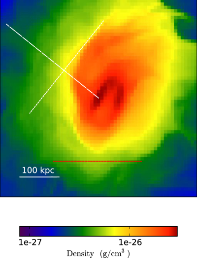
Figure 1: Density map on a slice through the cluster center. The dashed line shows the direction along which the profiles in Fig. 3 are computed, while the perpendicular dotted line–chosen to maximize line of sight velocity shear –indicates the observation direction for the solid red velocity PDF shown in Fig. 4. The dotted red line shows an alternate viewing direction with much less velocity shear; its velocity PDF is given by the thin red line in Fig. 3.

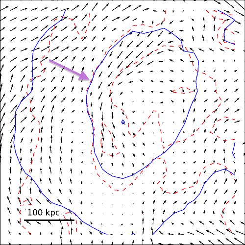
Figure 2: Velocity fields on the same slide as in Fig. 1, overlaid with density (solid blue curves) and temperature (dashed red curves) contours. The large purple arrow indicates the location of the cold front.

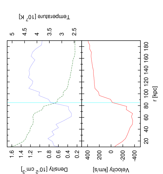
Figure 3: Density (dashed curve), temperature (dotted curve) and line-of-sight velocity (solid curve in the bottom panel) profiles along the a direction perpendicular to the cold front, as indicated in Fig. 1 with a dashed line. Here, the position of the cold front is given by the vertical (cyan) line at 85 kpc.

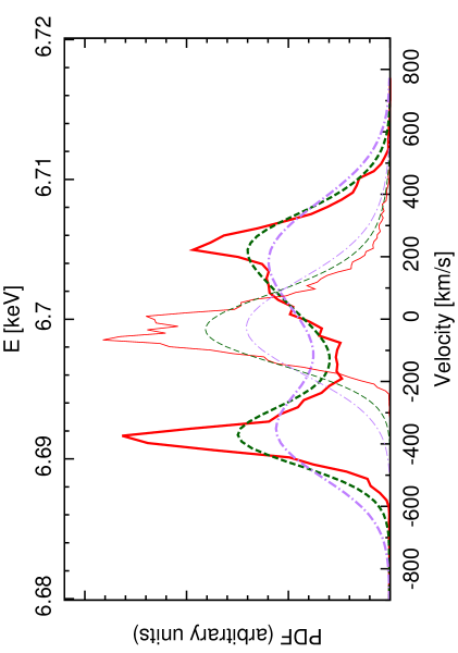
Figure 4: The thick solid (red) curve is the normalized emission-weighted velocity PDF from a box centered on the dotted line in Fig. 1. The box is 100 kpc long, 100 kpc wide and 1 Mpc deep. The thick dashed green curve, is the corresponding profile of the He-like iron line at 6.7 keV (see top axis for energy scale), including the effects of thermal broadening, while the thick dot-dashed purple curve also includes instrumental broadening. The thin lines show the same curves for the line of sight given by the dotted red line in Fig. 1.

Thus far, most constraints on gas bulk motions comes from observations of sharp density gradients in the plane of the sky. Classic bow shocks have been seen in a handful of violent mergers. Much more common are “cold fronts” (Markevitch & Vikhlinin, 2007): sharp contact discontinuities between gas phases of different entropies, discovered in the last decade thanks to the high-resolution of the Chandra X-ray telescope. They are seen both in mergers (where the cold gas arises from the surviving cores of infalling subclusters) and relaxed cool core clusters (where they are produced by the displacement and subsequent sloshing of the low-entropy central gas in the gravitational potential well of the cluster). They are remarkably ubiquitous, even in relaxed cool core clusters with no signs of recent mergers, which often exhibit several such cold fronts at different radii from the density peak. For instance, they are seen in more than half of all cool core clusters; given projection effects, most if not all cool core clusters should exhibit such features. Evidently, coherent gas bulk motions are extremely common if not universal, and their effects must be taken into account when interpreting Astro-H spectra. Generically, we would expect bulk motions to offset the centroids of emitting regions with significant line-of-sight relative velocity. Cold fronts have been used to probe the amplitude and direction of gas motions in the plane of the sky; combining this with line-of-sight information from the spectrum could prove very powerful indeed.

Our example is taken from an adiabatic numerical simulation from cosmological initial conditions with the adaptive mesh code Enzo (Bryan, 1999; Norman & Bryan, 1999; O’Shea et al., 2004). We assume a $\Lambda$CDM cosmology with cosmological parameters consistent with the seventh year WMAP results (Komatsu et al., 2011): $\Omega_{m}=0.274$, $\Omega_{\Lambda}=0.726$, $\Omega_{b}=0.045$, $h=0.705$, $\sigma_{8}=0.810$, $n_{s}=0.96$. The simulation has a box size of 64 Mpc, and a root grid of $128^{3}$. We picked the most massive cluster ($M\sim 2\times 10^{14}~{}\rm M_{\odot}$) from the fixed-grid initial run, and re-simulate it with much higher resolution. The highest spatial resolution is 11 kpc in the cluster center.

The cluster has a disturbed morphology, and shows a “cold front”-like feature in the core. Note that our adiabatic simulation necessarily produces a NCC cluster. The density and velocity fields on a slice through the cluster center are shown in Fig. 1 and 2, respectively. In the position indicated by the large arrow in Fig. 2, the density, temperature and velocity all change rapidly. This is clearly shown in Fig. 3, which shows density, temperature and velocity profiles along a line perpendicular to the front (indicated in Fig. 1 with a dashed line). At $\sim 85$ kpc from the cluster center, the density decreases while the temperature increases rapidly, as expected in a cold front (for a shock, the temperature jump would be opposite). Furthermore, the pressure is continuous across the front, while the tangential velocity changes direction discontinuously across the front—both well-known features of cold fronts (Markevitch & Vikhlinin, 2007).

For an observation direction along the white dotted line in Fig. 1, Fig. 4 shows the emission-weighted probability distribution function (PDF) of the line-of-sight velocity. Motivated by Table 2, we extract the emission-weighted PDF from an volume with an area of $100\times 100~{}{\rm kpc}^{2}$ and a depth of 1 Mpc (this last number represents the line of sight depth, and is chosen for convenience. Our results are insensitive to it as long as it is much larger than the core size, where most of the photons come from). The PDF clearly shows two peaks, centered at -400 ${\rm km\,s^{-1}}$ and 250 ${\rm km\,s^{-1}}$, corresponding to the gas on different side of the cold front. After convolution with thermal broadening, the dashed line shows the profile of the He-like iron line at 6.7 keV, while the dot-dashed line also includes the instrumental broadening of Astro-H. They also clearly show double peak features.

The above case is a somewhat idealized “best case” scenario, where we have assumed the viewing angle to be along the direction of maximum line of sight velocity shear, thus maximizing the separation between the two peaks in the velocity PDF. For a more general viewing angle, the separation would not be so clear, as we show with the thin curves in Fig. 4. This is the PDF along the red dotted curve in 1, which has very small line-of-sight bulk flow. There is only one large peak, but with a long tail. From Fig. 2, we see this long tail comes from the gas surrounding the cold clump, which has shear velocities with large components along the LOS. Therefore the PDF can also be separated into two components – a narrow component emitted by the cold clump and a broad component from the ambient gas. The offset between the components is a measure of the LOS contact discontinuity in the bulk velocity, while smaller scale shear contributes to the width. Such a decomposition of the line-of-sight velocity, combined with spatially resolved temperature and density information in the plane of the sky from X-ray imaging, could shed more light on the 3D velocity field as well as physical information such as the gas viscosity.

2.2 Volume-filling Factor of Turbulence

The previous section highlighted a situation where strong shear or bulk motion gives rise to different components with offset centroids (“separation driven” case). Another regime where different components could arise is when the two components have markedly different widths (“width driven” case). We saw an example of this at the end of the previous section: a narrow component due to a cold, kinematically quiescent clump, and a broader component due to the sheared surrounding ambient gas. More generally, different widths arise when turbulence varies spatially. The case when turbulence is only partially volume-filling is a particularly interesting special case. Many of the physical effects of turbulence depend not only on its energy density, but its volume filling fraction $f_{\rm V}$, which is often implicitly assumed to be unity. For instance, for turbulence to stave off catastrophic cooling, it must be volume-filling. This is by no means assured. For instance, analytic models (Subramanian, Shukurov & Haugen, 2006) of turbulence generation during minor mergers predict $f_{\rm V}\sim 0.2-0.3$ to be small, but area-filling (i.e., the projection of turbulent wakes on the sky cover a large fraction of the cluster area, $f_{\rm S}\sim O(1)$). Interestingly, cosmological AMR simulations which use vorticity as a diagnostic for turbulence find good agreement; $f_{\rm V}~{}\hbox to0.0pt{$<$\hss}{\lower 4.30554pt\hbox{$\sim$}}0.3$ and $f_{\rm S}\sim O(1)$ for all runs (Iapichino & Niemeyer, 2008). In our own simulations of stirring by galaxies (Ruszkowski & Oh, 2011), we have seen both high and low values of $f_{\rm V}$, depending on modeling assumptions. If $g$ modes are excited by orbiting galaxies (which requires the driving orbital frequency $\omega$ to be less than the Brunt-Väisälä  frequency $\omega_{\rm BV}$–a requirement which depends on both the gravitational potential and temperature/entropy profile of the gas), then volume-filling turbulence is excited; otherwise turbulence excited by dynamical friction is potentially confined to thin “streaks” behind galaxies (see also Balbus & Soker (1990); Kim (2007)). If turbulence is patchy, we might expect spectral lines to have a narrow thermal Doppler core (produced in quiescent regions), with turbulently broadened tails. In the context of our mixture model, measuring the fraction of photons in the second component might allow a quantitive measure of $f_{\rm V}$.

Yet another context in which strongly spatially varying or partial volume-filling turbulence could result in multiple components in the velocity PDF is AGN feedback, which is ubiquitous in most cool core clusters (Birzan et al. (2004); for a recent review, see McNamara & Nulsen (2012)). AGN jets are launched over a narrow solid angle and are fundamentally anisotropic; thus, their ability to sustain isotropic heating in the core has often been questioned. Isotropization of the injected energy could arise from weak shocks and sound waves (Fabian et al., 2003), frequent re-orientation of jets by randomly oriented accretion disks (King & Pringle, 2007), jet precession (Dunn, Fabian & Sanders, 2006; Gaspari et al., 2011), and cavities being blown about by cluster weather (Brüggen, Hoeft & Ruszkowski, 2005; Heinz et al., 2006; Morsony et al., 2010). As above, AGN could also excite g-mode oscillations; an intriguing example is a cross-like structure on 100 kpc scales in the ICM surrounding 3C 401 (Reynolds, Brenneman & Stocke, 2005). A measurement of $f_{\rm V}$ could thus constrain the efficacy of such mechanisms in isotropizing AGN energy deposition throughout the core. The expansion of AGN-driven cavities can also introduce high bulk velocities and shear (corresponding more to the “separation-drive” regime); this is potentially directly measurable with ATHENA’s excellent angular and spectral resolution (Heinz, Brüggen & Morsony, 2010), but would require indirect methods such as mixture modeling with the poor angular resolution of Astro-H. In §5, we analyze an AGN feedback simulation kindly provided to us by M. Brüggen.

2.3 Physical Significance of Mixture Model Parameters

In §3, we lay out our methodology for recovering mixture model parameters, and in subsequent sections we describe how accurately these can be constrained. These parameters are the mixture weights $f_{i}$, and means and variances $\mu_{i},\sigma_{i}^{2}$, of the fitted Gaussians. Given the results of this section, we can tentatively ascribe physical significance to these parameters. The mixture weights $f_{i}$ represent the emission-weighted fraction of the volume in each distinguishable velocity component. The Gaussian means $\mu_{i}$ represent the bulk velocity of a given component. In particular, the difference between the means is a measure of the LOS shear between these components (e.g., as arises at a cold front). Note that this shear due to bulk motions can be considerably larger than the centroid shift due to variance in the mean, induced by turbulent motion with a finite coherence length. The latter is given by $\mu_{i}\sim\sigma_{i}/\ \sqrt{N}$, where $N\sim L_{\rm emit}/l_{\rm v}$ is the average number of eddies pierced by the line of sight, and $L_{\rm emit},l_{\rm v}$ are the size of the emitting region and the coherence length of the velocity field respectively (Rebusco et al., 2008; Zhuravleva et al., 2012). The variances $\sigma_{i}$ represents turbulent broadening or shear due to the small scale velocity field.

3 Methodology

We have argued that the X-ray spectrum from galaxy clusters should have multiple distinct components. Uncovering these components is the domain of mixture modeling, a mature field of statistics with a large body of literature. We will specialize to the case of Gaussian mixture modeling, when Gaussians are used as the set of basis functions for the different components. This is an obvious choice, since thermal and instrumental broadening are both Gaussian, and turbulent broadening can be well approximated with a Gaussian when the injection scale is much smaller than the size of the emitting regions (Inogamov & Sunyaev (2003); i.e., once coherent bulk motions have been separated out by classification into different mixtures, the remaining small scale velocity field is well approximated by a Gaussian). It is also by far the best studied case. Mixture modeling has been applied to many problems in astrophysics, such as detecting bimodality in globular cluster metallicities (Ashman, Bird & Zepf, 1994; Muratov & Gnedin, 2010) linear regression (Kelly, 2007), background-source separation (Guglielmetti, Fischer & Dose, 2009), and detecting variability in time-series (Shin, Sekora & Byun, 2009), though to our knowledge it has not been applied to analyzing spectra. It should be noted that the specialization to Gaussian mixture is not necessarily restrictive; for instance, Gaussian mixtures have been used to model quasar luminosity functions (Kelly, Fan & Vestergaard, 2008). For us, the fact that Gaussians are a natural basis function allows us to model the spectra compactly with a small number of mixtures, and assign physical meaning to these different components.

Consider a model in which the observations $x_{1},\ldots,x_{n}$ are distributed as a sum of $k$ Gaussian mixtures:

$$f(x|\theta)=\sum^{k}_{j=1}\omega_{i}f_{j}(x|\mu_{j},\sigma^{2}_{j}),$$ (1)

where $f_{j}(x|\mu_{j},\sigma^{2}_{j})$ are normal densities with unknown means $\mu_{j}$ and variances $\sigma_{j}^{2}$, and $\omega_{i}$ are the mixture weights. The parameters which must be estimated for each mixture are therefore $\theta_{j}=(\omega_{j},\mu_{j},\sigma_{j}^{2})$, and the function $f$ can be viewed as the probability of drawing a data point with value $x$ given the model parameters $\theta$. Parameter estimation in this case suffers from the well-known missing data problem, in the sense that the information on which distribution $j$ a data point $x_{i}$ belongs to has been lost. In addition, the number of mixtures $k$ may not be a priori known. Standard techniques for overcoming this are a variant of maximum likelihood techniques known as Expectation Maximization (EM; Dempster, Laird & Rubin (1977)), or Maximum a Posterior estimation (MAP; see references in Appendix), which generally involves Markov Chain Monte Carlo (MCMC) sampling from the posterior. They are both two-step iterative procedures in which parameter estimation and data point membership are considered separately. Since they do not require binning of the data, all information is preserved. We have experimented extensively with both. However, due to the large number of data points ($\sim 10^{4}$ photons) in this application, we have found that the much simpler and faster procedure of fitting to the binned data yields virtually identical results. In the Appendix, we describe our implementation of Gibbs sampling MAP and how it compares with the much simpler method we use in this paper.

Here, we simply bin the data and adopt as our log-likelihood the C-statistic (Cash, 1979):

$$-2{\rm ln}{\cal L}(p|d)=-2\sum_{i=1}^{N_{bin}}n_{i}{\rm ln}e_{i}-e_{i}-{\rm ln}n_{i}!$$ (2)

where ${\cal L}(p|d)$ is the likelihood of the parameters $p$ given the data $d$, $N_{bin}$ is the number of bins, $n_{i}$ and $e_{i}$ are the observed and expected number of counts in the i-th bin; $n_{i},e_{i}$ are obviously functions of the data $d$ and the unknown model parameters $p$ respectively. It assumes that the number of data points in each bins is Poisson distributed (indeed, it is simply the log of the Poisson likelihood). As we describe in the Appendix, maximizing this statistic produces identical results to more rigorous mixture modeling techniques for large number of data points, when the bin size is sufficiently small. Naively, for a large number of data points one might expect $\chi^{2}$ minimization to work equally well. However, in fitting distributions we are sensitive to the wings of the Gaussian basis functions, when the expected number of counts in a bin is small and the data is therefore Poisson rather than Gaussian distributed.

With the likelihood specified in Equation 2, we sample from the posterior using Metropolis-Hastings MCMC, adapted from CosmoMC (Lewis & Bridle, 2002). Each run draws $\sim 10^{5}$ samples. The first 30% are regarded as burn-in and are ignored in the post-analyses. For all the runs, we visually exam the trace plots to check for convergence. The MCMC analysis yields the best-fit MAP parameters as well as the full posterior distribution of parameters, which allows us to estimate confidence intervals. In all cases, we use non-informative (uniform) priors; the range of possibilities for the turbulent velocity field is sufficiently large that only very weak priors are justifiable. The only obvious prior we use is $0<f_{i}<1$. Note that there are two identical modes in the likelihood, since it is invariant under permutation of the mixture indices–the well-known identifiability or “label-switching” problem. Generally, in a $k$ component mixture, there are $k!$ identical modes in the likelihood. During the course of a Monte-Carlo simulation, instead of singling out a single mode of the posterior, the simulation may visit portions of multiple modes, resulting in a sample mean which in fact lies in a very low probability region, as well as an unrealistic probability distribution. We enforce identifiability in a very simple manner by demanding $\mu_{1}<\mu_{2}$ and hence $s\equiv\mu_{2}-\mu_{1}>0$. While this is known to sometimes be problematic (Celeux, Hurn & Robert, 2000; Jasra, Holmes & Stephens, 2005), in practice it suffices for our simple models.

For a large number of data points, the distribution of model parameters becomes asymptotically Gaussian, in which case the Fisher matrix can be used to quickly estimate joint parameter uncertainties (e.g., Tegmark, Taylor & Heavens (1997)). As a consistency check, we therefore also calculate the Fisher matrix whenever the input model is simple enough to be expressed analytically. It is defined as:

$$F_{ij}=-\left<\frac{\partial^{2}\ln{\cal{L}}}{\partial p_{i}\partial p_{j}}\right>,$$ (3)

where $p_{i}$ is the i-th model parameter. The best attainable covariance matrix is simply the inverse of the Fisher matrix,

$$C_{ij}=(F^{-1})_{ij},$$ (4)

and the marginalized error on an individual parameter $p_{i}$ is $\sqrt{(F^{-1})_{ii}}$. Differences between the MCMC and the Fisher matrix error bars generally indicate the non-Gaussianity of the likelihood surface (or equivalently, that the log-likelihood cannot be truncated at second order in a Taylor expansion).

4 Idealized Models

4.1 Two component Gaussian mixture models: General Results

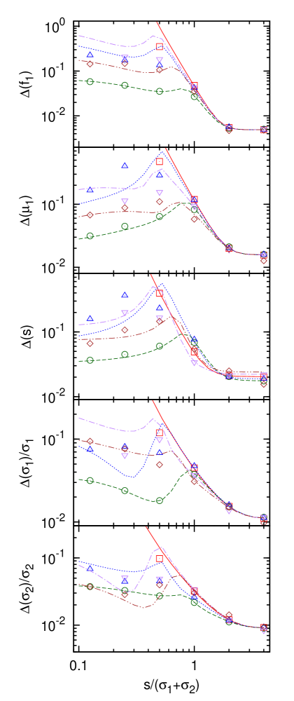
Figure 5: Constraints on the five model parameters with $N_{d}=10^{4}$ data points, as a function of $s/(\sigma_{1}+\sigma_{2})$, where $s=\mu_{2}-\mu_{1}$ is the separation between the means. The curves and points are the results obtained using the Fisher matrix and MCMC methods, respectively. The dashed lines and circles [green], dotted lines and upward triangles [blue], solid lines [red], dot-dashed lines and downward triangles [purple] and dot-dot-dashed lines and diamonds [brown] correspond to $\sigma_{2}=(0.6,0.8,1,1.2,1.4)\sigma_{1}$, respectively.

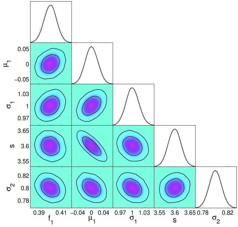
Figure 6: Error contours for a “SD” case ($\sigma_{1}=1$, $\sigma_{2}=0.8$, $s=2(\sigma_{1}+\sigma_{2})$): contours depict the 68%, 95% confidence levels for the marginalized distribution; the shadings shows the mean likelihood of the samples; the solid and dashed curves in the 1-D plots are the fully marginalized posterior and relative mean likelihood of the samples, respectively.

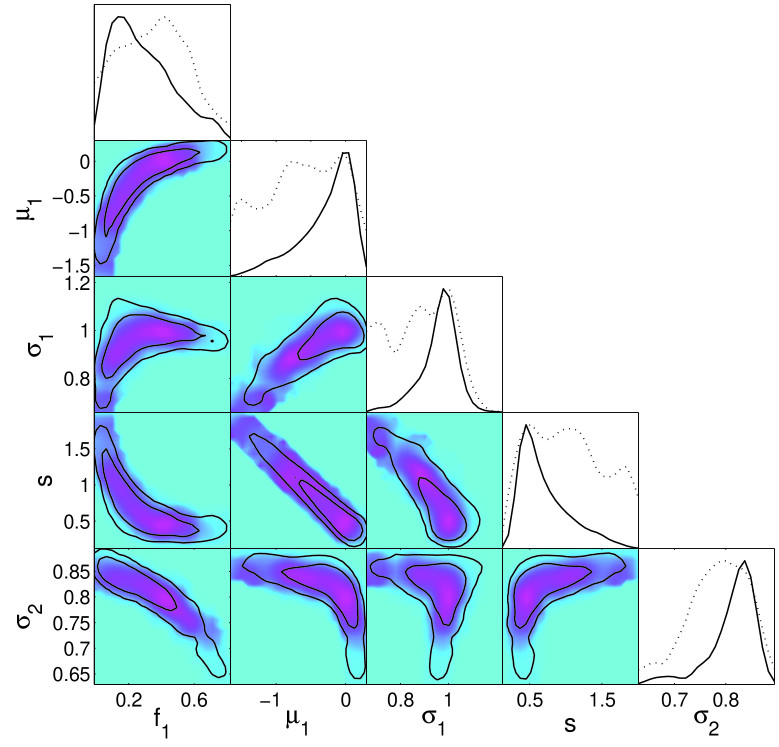
Figure 7: Same as Fig. 6 but for a “WD” case: $\sigma_{1}=1$, $\sigma_{2}=0.8$, $s=0.25(\sigma_{1}+\sigma_{2})$. Note the increased parameter degeneracies.

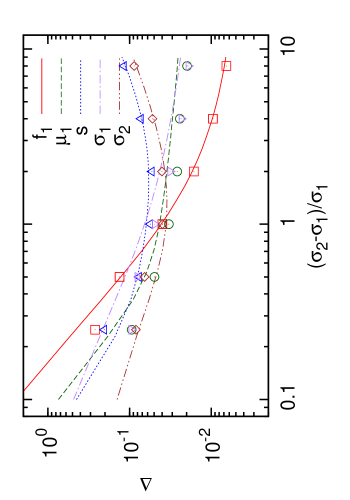
Figure 8: Constraints on the model parameters for a 2 Gaussian mixture as a function of the fractional difference in width, when $s=0.2$ and $\sigma_{1}=1$. As in Fig. 5, the lines and points show the results obtained with the Fisher matrix and MCMC technique, respectively. The solid lines and squares [red], dashed lines and circles [green], dotted lines and upward triangles [blue], dot-dashed lines and downward triangles [purple] and dot-dot-dashed lines and diamonds [brown] are the constraints on $f_{1}$, $\mu_{1}$, $s$, $\sigma_{1}$ and $\sigma_{2}$, respectively

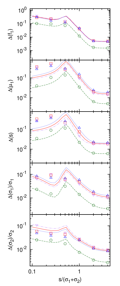
Figure 9: Constraints on the five free parameters for different values of $N_{d}$ and $f_{1}$. The solid curves and squares are the results for the fiducial case: $N_{d}=10^{4}$, $\sigma_{1}=1$, $\sigma_{2}=1$ and $f_{1}=0.4$; results for $N_{d}=10^{5}$, $f_{1}=0.3$, and $f_{1}=0.5$ are shown with dashed curves and circles, dotted curves and downward triangles, and dot-dashed curves and upward triangles, respectively.

Before focusing on the specific application to galaxy clusters, we first consider a more general problem: how well two Gaussian profiles can be separated. As mentioned previously, Astro-H data quality is generally only sufficient to allow solving for the two most dominant mixtures. A two mixture component is likely the most common scenario, with the most straightforward physical interpretation. These results serve to guide and motivate our later discussions.

Consider therefore the profile:

$$p(x)=\sum_{i=1,2}f_{i}G(x-\mu_{i},\sigma_{i}),$$ (5)

where $f_{i}$ is the fraction of each component, while $\mu_{i}$ and $\sigma_{i}$ are the mean and standard deviation of i-th Gaussian function. Given the constraint $\sum f_{i}=1$, there are only five model parameters, which we choose to be: $f_{1}$, $\mu_{1}$, $s(\equiv\mu_{2}-\mu_{1})$, $\sigma_{1}$ and $\sigma_{2}$. Note, $\mu_{2}$ has been replaced by $s$ (the separation between the two Gaussians) since the latter, as we will see more clearly later, usually carries clearer physical meaning.

The constraints, expressed in term of standard deviations $\Delta$ throughout this paper, are forecasted with both the MCMC and Fisher matrix methods (for the MCMC runs, they correspond to $68\%,95\%$ confidence intervals for $\Delta,2\Delta$ respectively, even if the parameter distribution is non-Gaussian). For each model we create a Monte-Carlo realization with $N_{d}$ data points and forecast constraints for this data set. Motivated by Table 2, we assume $N_{d}=10^{4}$. In general, the standard deviation of the model parameters $\Delta p\propto 1/\sqrt{N_{\rm d}}$, though there are some subtleties—see further discussions below. The constraints also depend on how much the two components differ; if they are difficult to distinguish, mixture modeling will fail. For Gaussian components, they may differ in fraction $f_{i}$, mean $\mu_{i}$ or width $\sigma_{i}$. Here, we shall mostly focus on a situation when the mixing fractions are comparable: $f_{1}=0.4,f_{2}=0.6$, and focus on how mixture separation can be driven by differences in mean (“separation dominated”, or SD), or width (“width drive”, or WD). In practice, we care mostly about the case when the mixing fractions are roughly comparable, since then the different components are of comparable importance in reconstructing the (emission-weighted) velocity field. As a practical matter, it also becomes increasingly difficult to perform mixture modeling when one component dominates (though see §4.4).

The results are shown in Fig. 5 - 9. Fig. 5 shows the constraints as a function of the separation $s=\mu_{2}-\mu_{1}$, normalized by the sum of the standard deviations: $s/(\sigma_{1}+\sigma_{2})$. Different line types and point types indicate different values of $\sigma_{2}=(0.6,0.8,1,1.2,1.4)\,\sigma_{1}$. Note that all five parameters scale with $s/(\sigma_{1}+\sigma_{2})$ in the same way, with fractional errors which are all roughly comparable. We can identify three distinct regimes:

• Separation Driven For $s/(\sigma_{1}+\sigma_{2})~{}\hbox to0.0pt{$>$\hss}{\lower 4.30554pt\hbox{$\sim$}}2$, the fractional errors converge to an asymptotic constant value, independent of $s/(\sigma_{1}+\sigma_{2})$. In this regime, the separation is so large that different components could be viewed as individually constrained without mixing from other components. Except for $\Delta(s)$ (which depends on $\Delta(\mu_{2})\sim\sigma_{2}/\sqrt{f_{i}N_{d}}$), this asymptotic convergence is also independent of $\sigma_{2}$ (i.e., the relative widths of the distributions don’t matter when the separation is large). The asymptotic values for $\Delta(\mu_{i})$, $\Delta(\sigma_{i})/\sigma_{i}$ and $\Delta(f_{i})$ are $\sigma_{i}/\sqrt{f_{i}N_{d}}$, $1/\sqrt{2f_{i}N_{d}}$ and $\sqrt{{f_{i}(1-f_{i})}/{N_{d}}}$, respectively; given our $N_{d}=10^{4}$, this corresponds to $\sim 1\%$ accuracy in parameter constraints.

• Hybrid For $0.3~{}\hbox to0.0pt{$<$\hss}{\lower 4.30554pt\hbox{$\sim$}}s/(\sigma_{1}+\sigma_{2})~{}\hbox to0.0pt{$<$\hss}{\lower 4.30554pt\hbox{$\sim$}}2$, the separation is comparable to the sum of widths. The mixing between different components become severe and the quality of parameter constraints decrease rapidly with decreasing $s$. Since constraints are increasing driven by data points in the tails of the respective mixtures (which drive distinguishability), the effective number of data points $N_{\rm eff}<N_{d}$ falls. Strong parameter degeneracies also develop.

• Width Driven When $s/(\sigma_{1}+\sigma_{2})~{}\hbox to0.0pt{$<$\hss}{\lower 4.30554pt\hbox{$\sim$}}0.3$, the separation between the distribution becomes negligible, and component separation is driven almost entirely by differences in width (note how parameter uncertainties blow up at low $s$ when $\sigma_{1}=\sigma{2}$). It is driven to an asymptotic value determined by the effective number of data points in the tails of the mixtures, $N_{\rm eff}$.

The results obtained with the Fisher matrix (lines) and MCMC (points) agree well with each other when the mixtures are easily distinguishable (when $s/(\sigma_{1}+\sigma_{2})$ is large or $\sigma_{2}/\sigma_{1}$ is reasonably far away from 1). Otherwise, discrepancies between these two methods are clear. These discrepancies are caused by the non-Gaussianity of the likelihood surfaces and the priors we placed in the MCMC runs. In this regime, one therefore cannot use the Fisher matrix approximation to the full error distribution.

Fig. 6 and 7 show the marginalized likelihood distributions and error contours for two example runs. Fig. 6 is in the SD regime ($s=2(\sigma_{1}+\sigma_{2})$). The likelihood distributions are very close to Gaussian, explaining the consistency between the Fisher matrix and MCMC results. The contours allow direct reading of correlations among parameters. The strongest correlation is between $\mu_{1}$ and $s$. As expected, they are negatively correlated, since $s=\mu_{2}-\mu_{1}$ while the $\mu_{i}$’s are uncorrelated. Fig. 6 is in the WD regime ($s=0.25(\sigma_{1}+\sigma_{2})$). The likelihood distributions now deviate from Gaussians, and the correlations among parameters are much stronger. These are all consistent with the facts that the constraints are worse (due to larger parameter degeneracies) and the Fisher matrix results are no long in agreement with MCMC results (due to non-Gaussianity of the likelihood surface).

In Fig. 8, we show how the constraints vary with differences in the Gaussian width in the “width dominated” regime. The width of the first component is fixed to $\sigma_{1}=1$, while the separation $s=0.2$ (note that $s/(\sigma_{1}+\sigma_{2})\sim 0.2$ is typically the minimal value expected in cluster turbulence when there are no bulk flows, and is due solely to error in the mean; see §2.3). In general, the constraints improve as the differences in width increase, consistent with intuitive expectations. However, the constraints on $s$ and $\sigma_{2}$ turn over around $\sigma_{2}\sim 2\sigma_{1}$, beyond which they increase with $\sigma_{2}$. This can be understood as follows: the error on these quantities receive contributions from confusion error (which dominates at low $\sigma_{2}$) and scaling with $\sigma_{2}$ (since $\Delta(\mu_{i})\sim\sigma_{i}/\sqrt{f_{i}N_{d}}$ and $\Delta\sigma_{i}\sim\sigma_{i}/\sqrt{2f_{i}N_{d}}$; this dominates at high $\sigma_{2}$). On the other hand, the error on the mixing fraction $f_{1}$ scales strongly with the difference in widths, since it is driven solely by confusion error. However, for other parameters the scaling is significantly weaker. For most cluster scenarios, the width-driven regime gives relative errors of $\Delta p/p\sim 10\%$, which is still small.

Fig. 9 shows how the constraints vary with $N_{d}$ and $f_{1}$. The fiducial case (solid curves and squares) is computed assuming $N_{d}=10^{4}$, $\sigma_{1}=1$, $\sigma_{2}=0.8$ and $f_{1}=0.4$, exactly the same as the dotted curves and upward triangles in Fig. 5. As we increase the $N_{d}$ by a factor of 10, most constraints are improved by a factor of $\sqrt{10}$, consistent with our expectation that $\Delta p_{i}/p_{i}\propto 1/\sqrt{N_{d}}$. This is despite the fact that only in the asymptotic SD case are relative errors quantitatively given by the Poisson limit $\Delta p_{i}/p_{i}\approx 1/\sqrt{(f_{i}N_{d})}$. This is because when mixtures overlap and are in the hybrid/WD regimes, results are driven by the distribution tails, where the effective number of data points is still $N_{\rm eff}\propto N_{\rm d}$. For $s$ and $\mu_{1}$, however, MCMC results show better improvements in the WD regime than factors of $\sqrt{10}$. This might be due to reduced parameter degeneracies from the larger number of data points. Varying $f_{1}$ to 0.3 and 0.5 mildly impacts the results. As the $f_{1}$ goes closer to 0.5, constraints improve for most parameters, except for $f_{1}$ and $\sigma_{2}$. Constraints on $f_{1}$ are almost unchanged while constraints on $\sigma_{2}$ are degraded, because fewer data points are available in the second component to constrain $\sigma_{2}$.

Based on Fig. 5 and 8, we can already anticipate the constraints from Astro-H: when there is significant bulk flow and the modes have a large relative velocity $v_{\rm bulk}>\sigma_{\rm turb}$, parameters can be constrained to $\sim 1\%$ accuracy (SD regime); when the relative velocity is small but the widths are different by a reasonable (a few tens of percents) amount, the parameter estimates are accurate at the $\sim 10\%$ level (WD regime). Given the modeling uncertainties in the physical interpretation of these parameter estimates, such accuracy is more than adequate. Next, we will consider two specific examples of the SD regime and WD regime respectively.

4.2 Application to Clusters: the Single Line Scenario

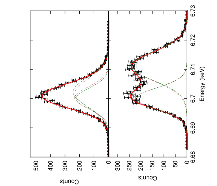
Figure 10: The mock spectra (data points) and best-fit models for the WD (upper panel) and SD (lower panel) cases in the single line scenario. The red solid and dot-dashed lines are the input overall spectra and individual components respectively. The green dashed lines are the recovered components. The recovery is remarkably accurate, even when (as in the top panel) the spectra is visually indistinguishable from a single component Gaussian.

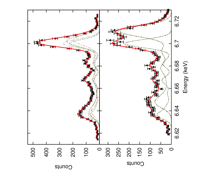
Figure 11: Same as Fig. 10 but for the entire iron line complex. The continuum has also been included, assuming a metallicity of 0.3 ${\rm Z_{\odot}}$.

Table 3: Input parameters for the WD case and recovered best-fit parameters together with their 1-$\sigma$ errors. Also shown are the predicted uncertainties using the Fisher matrix technique. Note that $v_{\rm pec},v_{\rm rel}$ are line of sight quantities, while $v_{\rm tb,1},v_{\rm tb,2}$ are 3D velocity dispersions (assuming $v_{\rm 3D}^{2}=3v_{\rm 1D}^{2}$).

		$f_{1}$	$v_{pec}$(km/s)	$v_{rel}$(km/s)	$v_{tb,1}$(km/s)	$v_{tb,2}$(km/s)
	Input	0.4	0	100	150	300
Single line	MCMC	$0.46_{-0.12}^{+0.18}$	$11.34_{-11.32}^{+11.62}$	$89.48_{-13.85}^{+28.06}$	$164.89_{-33.97}^{+33.75}$	$298.82_{-13.34}^{+11.43}$
	Fisher Matrix	(0.12)	(12.99)	(14.06)	(37.03)	(10.75)
Multiple lines	MCMC	$0.42_{-0.09}^{+0.25}$	$-14.24_{-9.79}^{+17.15}$	$130.72_{-11.19}^{+65.05}$	$145.48_{-33.65}^{+42.59}$	$291.64_{-34.19}^{+5.40}$
	Fisher Matrix	(0.12)	(11.28)	(17.37)	(36.75)	(10.65)
Multiple lines	MCMC	$0.64_{-0.13}^{+0.22}$	$5.44_{-9.08}^{+18.10}$	$147.88_{-34.85}^{+124.25}$	$180.16_{-21.43}^{+26.58}$	$308.14_{-83.92}^{+13.44}$
plus continuum	Fisher Matrix	(0.19)	(15.36)	(27.04)	(53.07)	(17.19)

Table 4: Same as Table 3 but for the SD case.

		$f_{1}$	$v_{pec}$(km/s)	$v_{rel}$(km/s)	$v_{tb,1}$(km/s)	$v_{tb,2}$(km/s)
	Input	0.4	0	500	150	300
Single line	MCMC	$0.40_{-0.02}^{+0.01}$	$2.17_{-6.40}^{+7.28}$	$493.65_{-4.82}^{+4.54}$	$152.71_{-5.93}^{+7.62}$	$310.98_{-5.33}^{+6.65}$
	Fisher Matrix	(0.01)	(6.40)	(4.52)	(11.45)	(9.77)
Multiple lines	MCMC	$0.41_{-0.01}^{+0.01}$	$2.47_{-4.72}^{+6.18}$	$505.28_{-4.13}^{+3.96}$	$148.71_{-9.61}^{+14.19}$	$294.13_{-9.43}^{+8.84}$
	Fisher Matrix	(0.01)	(5.73)	(4.15)	(12.39)	(9.24)
Multiple lines	MCMC	$0.40_{-0.02}^{+0.02}$	$-0.01_{-8.19}^{+7.88}$	$486.43_{-4.98}^{+4.90}$	$167.92_{-16.89}^{+15.33}$	$309.75_{-14.03}^{+14.04}$
plus continuum	Fisher Matrix	(0.02)	(6.72)	(4.61)	(15.75)	(12.50)

We begin our discussion of mixture modeling of cluster emission line spectra with the simplest case. For now we ignore line blending and continuum emission, and only consider one emission line – the He-like iron line at 6.7 keV. Again, we assume the PDF is composed of two Gaussian components. Most of these assumptions will be relaxed later. We assume the cluster is isothermal with a temperature of 5 keV. The assumption of an isothermal distribution is of course somewhat crude for the entire cluster. However, for nearby clusters, the emission-weighted spectrum is accumulated from a small area where temperature variations are generally mild ($<0.5$ keV). Moreover, our results are not very sensitive to the temperature distribution. We express our results in terms of the bulk peculiar velocity of the first component ($v_{pec}$), the relative velocity between the two components ($v_{rel}$), and the 3D turbulent velocity dispersions of each component ($v_{\rm tb,1}$ and $v_{\rm tb,2}$). We assume isotropic turbulence, so the line of sight velocity dispersion is $v_{\rm tb,i}/\sqrt{3}$. They are related to the Gaussian PDF via:

$$\mu_{1} = \nu_{0}+\nu_{0}\frac{v_{pec}}{c},$$ (6)

$$s = \nu_{0}\frac{v_{rel}}{c},$$

$$\sigma_{i} = \sqrt{\sigma_{tb,i}^{2}+\sigma_{ther}^{2}+\sigma_{instr}^{2}},$$

$$\sigma_{tb,i} = \nu_{0}\frac{v_{tb,i}}{\sqrt{3}c},$$

$$\sigma_{ther} = \frac{\nu_{0}}{c}\sqrt{\frac{kT}{Am_{p}}},$$

where $\nu_{0}$ is the line frequency in the rest frame, $\sigma_{instr}$ is the standard deviation of instrumental noise (FWHM/2.35), $A$ is the atomic weight of iron and $m_{p}$ is the proton mass. In our WD example, we assume $(v_{\rm tb,1},v_{\rm tb,2})=(150,300)\,{\rm km\,s^{-1}}$, and $v_{\rm rel}=100\,{\rm km\,s^{-1}}$. For the SD example, we assume the same $v_{\rm tb,1},v_{\rm tb,2}$, but $v_{\rm rel}=500\,{\rm km\,s^{-1}}$. In all cases, we assume the bulk velocity zero-point $v_{\rm pec}=0\,{\rm km\,s^{-1}}$. Sloshing in the cluster potential well generally results bulk motions with transonic Mach numbers (Markevitch & Vikhlinin, 2007), so such a value is realistic for a 5 keV cluster (with sound speed $c_{\rm s}\sim 1000\,{\rm km\,s^{-1}}$) along an arbitrary line of sight—indeed, such velocities are found in the simulated cluster in §2.1. With these assumptions, the widths of the first and second component, including instrumental, thermal and turbulent broadening, are 3.54 and 4.87 eV; the offsets between peaks are 1.12 and 11.17 eV for the WD and SD cases, respectively. These parameter choices correspond to $s/(\sigma_{1}+\sigma_{2})=(0.13,1.3)$ respectively, and thus can be compared to expectations from Fig. 5. Note that the SD case is not quite in the asymptotic regime $s/(\sigma_{1}+\sigma_{2})~{}\hbox to0.0pt{$>$\hss}{\lower 4.30554pt\hbox{$\sim$}}3$ yet (where the relative errors would be $\sim 1/\sqrt{f_{i}N_{d}}\sim 1\%$), but it is fairly close.

The mock spectra and best-fit models for $10^{4}$ photons are shown in Fig. 10. The best-fit parameters and their uncertainties are listed in the first row of Table 3 and 4. In accordance with expectations from §4.1, component recovery is remarkably accurate. Even is the WD case, which is visually indistinguishable from a single Gaussian (see top panel of Fig. 10), the decomposition into the original mixtures is very good, and most velocities are constrained to within $\sim 10-30\,{\rm km\,s^{-1}}$, which is significantly higher accuracy than needed to model the physical effects of bulk motions and turbulence in the cluster. This showcases the great potential of high spectral resolution instruments. Of particular interest is the constraint on the mixing fraction, which is a very good indicator of our ability to separate different components. A confident detection of multiple components should have $f_{1}/\Delta(f_{1})$ larger than a few, i.e., the best-fit fraction should be at least a few $\sigma$ away from “non-detection” ($f_{1}$ or $f_{2}$ equal to 0). In the single line scenario, the $1-\sigma$ error of $f_{1}$ is 0.01 and 0.12 in the SD and WD cases, respectively, consistent with our expectations from discussions in the previous section. However, a large fraction of the constraints in the WD case is from the tails, and could easily be affected by continuum emission (see discussion below). Also note the general consistency between Fisher matrix and MCMC techniques, indicating the Gaussian shape of the likelihood surface for this scenario.

4.3 The Impact of Multiple Lines and Continuum

In this section, we consider the impact of multiple lines and continuum emission. Iron lines appear as a line complex between 6.6 and 6.75 keV, and these lines inevitably blend together. Multiple lines have two competing effects. First, taking all lines into account–all of which have identical mixture decompositions–means more photons, which reduces shot noise in parameter estimates. The photons from the entire line complex is about twice that from the He-like iron line alone. Secondly, as different lines blend together, information contained in the shape of individual lines is partly lost due to blending in the line wings. The latter are crucial to driving parameter estimation in the hybrid and WD cases (note however, from Fig. 11 that the lowest and highest energy lines in the complex have low/high energy line wings respectively which are unaffected by blending. This is particularly important in the case of the high energy He-like line, which is by far the strongest line in the complex). These two factors have opposite effects on the constraints. As in the previous sub-section, we run MCMC chains and Fisher matrices to estimate the constraints. The properties of the line complex were taken from ATOMDB database (v. 2.0.1). To save computing time, we only included the ten strongest lines lines. Fisher matrix estimates including more lines show negligible difference.

The results are listed in the second row of Table 3 and 4. In the SD case, the constraints estimated using both MCMC and Fisher matrix techniques are very close to those in the single line scenario, indicating almost total cancellation between the effects just mentioned. In the WD case, the constraints from the Fisher matrix technique are again close to the single line scenario. However, the results from MCMC runs show asymmetry, and in general, the constraints are worse than in the single line scenario. Line blending seems to make the likelihood surface significantly non-Gaussian.

Next, we include the effect of continuum emission. Continuum acts as a source of background noise. Even though we can measure and subtract the continuum, doing so introduces shot noise, particularly in the line wings when Fe line emission and continuum brightness can become comparable, or continuum emission could even dominate. The relative level of continuum and Fe line emission is controlled by metallicity; larger metallicities imply brighter lines. The mean metallicity of clusters is typically ${\rm Z}\sim 0.3\,{\rm Z_{\odot}}$, which we shall assume, though the metallicity in the cluster center is often higher due to contributions from the cD galaxy. We apply our mixture model incorporating both the effects of line blending and continuum; the results are shown in Table 3 and 4, and in Fig. 11 (for the purpose of clarity, only 1/3 of the data points are shown in this figure). The results are as one might expect. In the SD case, the constraints are only slightly worsened, since the mixtures are clearly separated, and almost all the $\sim f_{i}N_{d}$ points in a given mixture can be used for parameter estimates; only a small fraction in the line tails are contaminated by line blending and the continuum. The constraints in the WD case are more badly affected, since the constraints in this case are largely drawn from the tails; here, the differences between the MCMC and Fisher matrix techniques are also further enlarged. The presence of the continuum and line blending limit the domain of the WD regime, which is no longer strictly independent of $s/(\sigma_{1}+\sigma_{2})$. For instance, if we assume $v_{\rm rel}=50\,{\rm km\,s^{-1}}$ (corresponding to $s/(\sigma_{1}+\sigma_{2})=0.067$), the MCMC simulations fail to converge). They thus limit our ability to constrain components with small separations, though in practice such small separations should be rare.

4.4 Model Selection: When is a Mixture Model fit Justified?

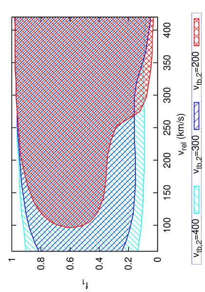
Figure 12: Model selection: regions of the $f_{1}$ - $v_{rel}$ plane where the double component model is preferred according to the BIC, for $v_{\rm tb,1}=100\,{\rm km\,s^{-1}}$, $v_{\rm tb,2}=(200,300,400)\,{\rm km\,s^{-1}}$, and $f_{1}=0.4$, $v_{\rm pec}=0\,{\rm km\,s^{-1}}$.

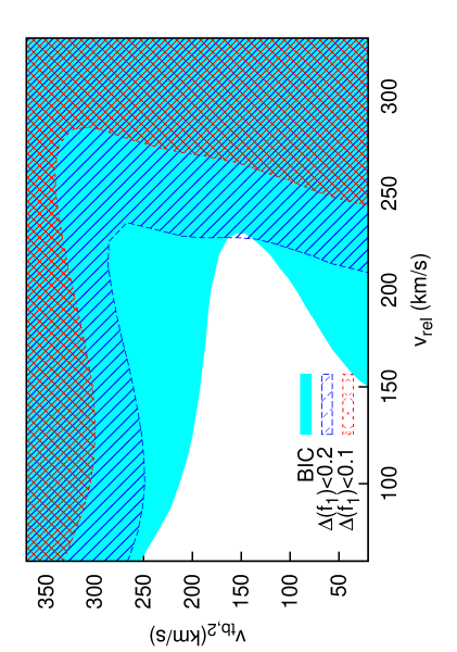
Figure 13: Model selection: shaded regions shows the regions of $(v_{\rm rel},v_{\rm tb,2})$ parameter space where the double component model is preferred according to BIC, while the hatched regions are where mixing fraction is accurately constrained: $\Delta(f_{1})<(0.2,0.1)$ (cyan and purple hatches respectively). All other parameters are as in Fig. 12.

Thus far, we have only considered how accurately mixture model parameters can be constrained. However, this begs the question of whether a mixture model approach is justified at all, particularly when (as in the WD case) the observed emission line is visually indistinguishable from a single Gaussian. Introducing additional parameters will always result in an improved fit, even when these parameters are largely irrelevant and of little physical significance. This is essentially a model selection problem. We use information criteria (e.g., see Liddle (2004)) which penalize models with more parameters, to identify preferred models. While they have solid underpinnings in statistical theory, fortunately, they have very simple analytic expressions. In this paper, we use the Bayesian Information Criterion (BIC; Schwarz (1978)):

$$BIC\equiv-2\ln{\cal L}_{\mathrm{max}}+k\ln N$$ (7)

where ${\cal L}_{\mathrm{max}}$ is the maximum likelihood achievable by the model, $k$ is the number of free parameters, and $N$ is the number of data points; the preferred model is one which minimizes BIC. The BIC comes from the Bayes factor (Jeffreys, 1961), which gives the posterior odds of one model against another. We use it over the closely related Akaike Information Criterion (AIC; Akaike (1974)), which places a lower penalty on additional model parameters. Thus, we adopt a conservative criterion for preferring mixture models. The absolute value of the BIC has no significance, only the relative value between models. A difference of 2 is regarded as positive evidence, and of 6 or more as strong evidence, to prefer the model with lower BIC (Jeffreys, 1961; Mukherjee et al., 1998). Note that the BIC does not incorporate prior information. This is possible with the more sophisticated notion of Bayesian evidence (e.g., Mackay (2003)), but involves expensive integrals over likelihood space, and is unnecessary in our case since we adopt uninformative priors.

We aim to distinguish the double component model with $k=5$ (free parameters: $(v_{\rm pec},v_{\rm rel},f_{1},v_{\rm tb,1},v_{\rm tb,2}$), against the single component model with $k=2$ (free parameters: $\mu,\sigma$). We create simulated data sets which have two underlying components, and see which regions of parameter space the BIC will correctly prefer the two component model. Our simulated line profiles incorporate the additional effects of thermal and instrumental broadening, continuum, and line blending. Rather than exploring the full 5 dimensional space, we explore the most interesting subspace to see where model selection is effective. In Fig. 12 we explore model selection in the $f_{1}$ - $v_{\rm rel}$ plane, for $v_{\rm tb,2}=(200,300,400)\,{\rm km\,s^{-1}}$, and $v_{\rm pec}=0\,{\rm km\,s^{-1}}$, $f_{1}=0.4$, $v_{\rm tb,1}=100\,{\rm km\,s^{-1}}$. The plot shows where the BIC for the double component fit is smaller than that for the single component fit (note that the BIC is obtained by allowing for variation in all fitted parameters; we are just plotting model selection in a subspace). When $v_{\rm tb,2}=400\,{\rm km\,s^{-1}}$, all values of $v_{\rm rel}$ and all $0.1<f_{1}<0.9$ permit correct selection of the double component model. The result is very similar for $v_{\rm tb,2}=300\,{\rm km\,s^{-1}}$, but for $v_{\rm tb,2}=200\,{\rm km\,s^{-1}}$, if both $f_{1},v_{\rm rel}$ assume low values, the double component model is not preferred. Overall, it is reassuring to see that model selection is not very sensitive to $f_{1}$, since we previously restricted our studies to $f_{1}=0.4$. Thus, even if a smaller fraction of the emission weighted volume has a markedly different velocity structure, it will be detectable in the spectrum. In Fig. 13, we show the regions of $(v_{\rm rel},v_{\rm tb,2})$ parameter space where the double component model is preferred according to BIC. Overall, as expected, the mixtures can be distinguished if $v_{\rm rel}$ or $v_{\rm tb,2}$ are large; for Astro-H and with the adopted parameters, this is of order $200\,{\rm km\,s^{-1}}$. In addition, we show the regions where the mixing fraction $f_{1}$ is accurately constrained to $\Delta(f_{1})<(0.1,0.2)$, since the error on the mixing fraction should be a good indicator of our ability to distinguish mixtures. We use the Fisher matrix formalism to calculate these constraints. The results are qualitatively similar that obtained with the BIC, though somewhat more restrictive.

4.5 Non-Gaussian Mixture Components

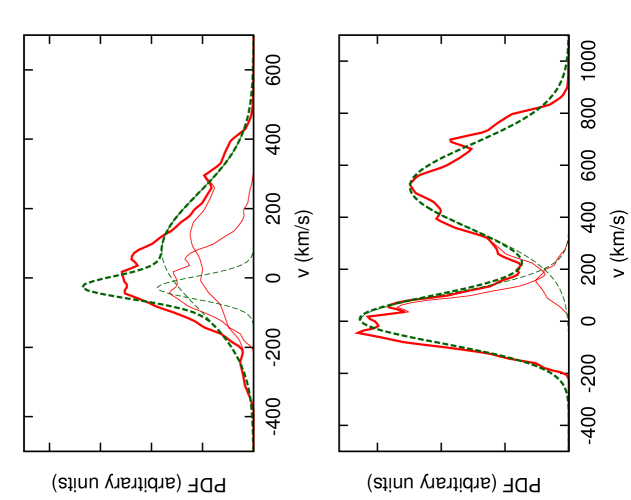
Figure 14: The velocity PDFs in the WD (upper panel) and SD (lower panel) cases. The solid (red) and dashed (green) curves are the input and recovered PDFs, respectively. The thick curves are the overall PDFs, while the thin curves show the individual components.

Table 5: Non-Gaussian mixture components: input parameters (obtained by shifting and rescaling the non-Gaussian mixtures) and recovered best-fit parameters together with their 1-$\sigma$ errors, for both the WD and SD cases, as in Fig. 14. Note that the Fisher matrix results–which require an analytic likelihood–assume Gaussian mixtures, and hence are the same as Tables 3 and 4.

		$f_{1}$	$v_{pec}$(km/s)	$v_{rel}$(km/s)	$v_{tb,1}$(km/s)	$v_{tb,2}$(km/s)
WD	Input	0.4	0	100	150	300
	MCMC	$0.17_{-0.01}^{+0.49}$	$-33.18_{-11.54}^{+37.53}$	$112.49_{-10.96}^{+89.48}$	$63.80_{-14.55}^{+138.51}$	$284.99_{-39.82}^{+4.86}$
	Fisher Matrix	(0.19)	(15.36)	(27.04)	(53.07)	(17.19)
SD	Input	0.4	0	500	150	300
	MCMC	$0.43_{-0.02}^{+0.01}$	$8.37_{-7.44}^{+5.83}$	$509.22_{-4.49}^{+4.49}$	$162.28_{-17.94}^{+12.09}$	$284.55_{-10.77}^{+13.81}$
	Fisher Matrix	(0.02)	(6.72)	(4.61)	(15.75)	(12.50)

All the preceding discussions are based on the assumption that the PDFs of individual components are Gaussian, which is not true in general. As we see in Fig. 4, individual mixtures show deviations from Gaussianity, i.e. Gaussians are a good but imperfect set of basis functions. In principle, this can be dealt with by fitting higher order mixture models, but in practice the data quality from Astro-H does not allow this; parameter estimation becomes unstable and large degeneracies develop, particularly since the higher order mixtures generally have low mixing fractions $f_{i}$. Unless their velocity means or widths are very different, the physical interpretation of these additional components is also more difficult. Here we construct a simple toy model to isolate the effects of non-Gaussian components. As there are many flavors of non-Gaussianity, the results we show are meant to be illustrative rather than definitive.

To this end, we extract PDFs from a simulated relaxed cluster, use them as the “basis” PDFs of individual components, resize and combine them to produce a composite PDF, which is in turn used to generate mock spectra. The “basis” PDFs are extracted from a simulation by Vazza et al. (2010), which the authors kindly made public; we sample different PDFs by looking along different lines of sight. The cluster, labeled as E14, has a mass of ${\rm M}\sim 10^{15}~{}\rm M_{\odot}$ and experienced its latest major merger at $z>1$. Due to shot noise which arises from the finite resolution (25 ${\rm kpc}\,h^{-1}$) of this simulation–which results in a small number of cells–we are forced to extract the emission weighted velocity PDFs from a large volume of $400\times 400\times 1000~{}{\rm kpc}^{3}$. The PDFs are shifted (to match means), linearly rescaled (to match variances) and combined to produce the same WD and SD cases in § 4.3. We then convolve the composite PDFs with thermal broadening and instrumental noise for the entire Fe line complex, and add continuum to produce mock spectra. Finally, we fit the mock spectra to separate and constrain the two components. The results are shown in Fig. 14 and Table 5. In Fig. 14, the solid (red) curves are the input PDFs while the dashed (green) curves are the best-fit model. The thick and thin curves are the total PDF and individual components, respectively (note that because we display the velocity PDF rather than the spectrum, the multiple lines in the Fe complex, as well as the continuum and thermal/instrumental broadening, are not shown. However, all these effects are included in the simulations). In the SD case (lower panel), the two components are recovered almost perfectly. In the WD case (upper panel), however, there are some discrepancies between the input and output PDFs. The same conclusion can be drawn from Table 5; in the WD case, the best-fit values of $f_{1}$ and $v_{tb,1}$ are somewhat different from the input values. However, they are still within the (large) errors. Comparing Table 5 with Table 3 and 4, we see that at least in this case, non-Gaussian components have limited effect on the results. Note the strong discrepancy between MCMC and Fisher matrix error bars in both cases, and in particular the strong asymmetry in MCMC errors. We repeated the same exercise several times with PDFs randomly drawn along different lines of sight from the same simulation. In most attempts, we are able to recover the input parameter values within the uncertainties. Thus, conclusions based on Gaussian components are still applicable when the true PDFs deviate from Gaussianity by a reasonable amount. Instrumental and thermal broadening, which gaussian, effectively smooth out small scale deviations from Gaussianity.

5 Results from Numerical Simulations

5.1 Cold Front Cluster

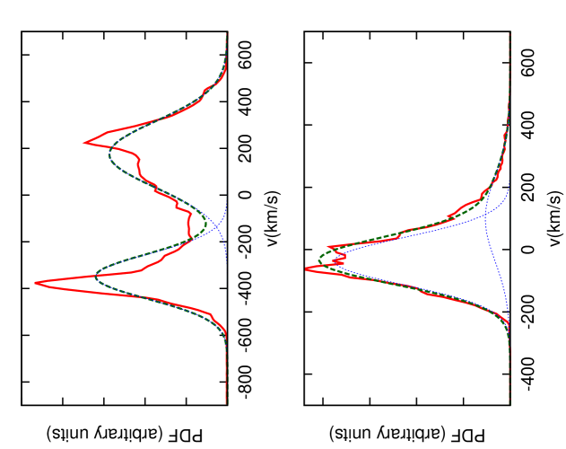
Figure 15: “Cold front” cluster: the solid (red) curves are the same velocity PDFs as in Fig. 4. The dashed (green) curves are the recovered PDFs from the best-fit models, and the dotted (blue) curves are the individual components. Numerical values of the fit parameters are in Table 6.

Table 6: “Cold front” cluster: best-fit parameters and their uncertainties for the PDFs in Fig. 15, obtained using the Enzo simulation described in §2.1. Case 1 and 2 are the top and bottom panels of Fig. 15 respectively. The “true values” are obtained by fitting the PDF directly, while the recovered values are obtained from the mock spectrum of $10^{4}$ photons, which includes line blending, thermal and instrumental broadening, and continuum emission.

		$f_{1}$	$v_{pec}$(km/s)	$v_{rel}$(km/s)	$v_{tb,1}$(km/s)	$v_{tb,2}$(km/s)
Case 1	True values	$0.40_{-0.01}^{+0.01}$	$-359.53_{-1.93}^{+1.73}$	$517.15_{-2.76}^{+2.24}$	$155.00_{-2.68}^{+2.49}$	$269.39_{-3.02}^{+4.04}$
	Recovered	$0.43_{-0.01}^{+0.01}$	$-348.67_{-6.00}^{+6.34}$	$522.79_{-4.82}^{+3.31}$	$165.52_{-16.27}^{+13.16}$	$247.04_{-9.66}^{+12.70}$
Case 2	True values	$0.78_{-0.02}^{+0.02}$	$-40.49_{-1.52}^{+1.70}$	$142.10_{-6.40}^{+11.28}$	$128.32_{-2.01}^{+2.17}$	$220.24_{-6.93}^{+4.22}$
	Recovered	$0.80_{-0.26}^{+0.11}$	$-37.14_{-13.42}^{+9.09}$	$136.29_{-60.12}^{+78.13}$	$131.28_{-38.74}^{+11.02}$	$237.73_{-53.31}^{+23.30}$

Finally, we apply our tool to cluster simulations. In the first example, we attempt to recover the velocity PDFs shown in Fig. 4, which derives from a cosmological ENZO simulation of a cold front cluster. These two cases, which come from different lines of sight through the same cluster, correspond to $s/(\sigma_{1}+\sigma_{2})={1.42}$ and $s/(\sigma_{1}+\sigma_{2})={0.42}$ respectively, i.e. in the “separation-driven” and “width-driven” regimes. We first fit the PDFs with a mixture model when no sources of noise or confusion are present, to derive the “true” parameter values. We then generate mock spectra by adding thermal and instrumental broadening, continuum emission and line blending to the PDFs, and then apply mixture modeling to the results. The results are given in Fig. 15 and Table 6. Overall, the results are very good. The best-fit models successfully recover the general features of the PDFs, and accurate parameter estimates with uncertainties which are consistent with our estimates from the toy models – on the order of $\sim 10\%$ for the width-drive case (case 2) and $\sim 1\%$ for the separation-driven case (case 1). No systematic biases appear to be present. As we discussed in §2.3, these parameters all have physical significance: $v_{\rm tb,i}$ relates to the turbulent energy density in each component, $f_{i}$ to the emission weighted volume fraction of each component, and $v_{\rm rel}$ to the bulk velocity shear between them. We also applied the single component model to the same mock spectra, and compared the BIC values. In both cases, the double component model is preferred (case 1: $BIC_{\rm double}-BIC_{\rm single}=-1002$; case 2: $BIC_{\rm double}-BIC_{\rm single}=-10$).

5.2 AGN Feedback Cluster

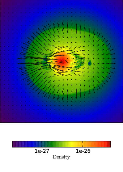
Figure 16: Density map and velocity field on the $y-z$ plane. The size of the figure is 1 Mpc; the bulk motion along the y-direction has been substracted out.

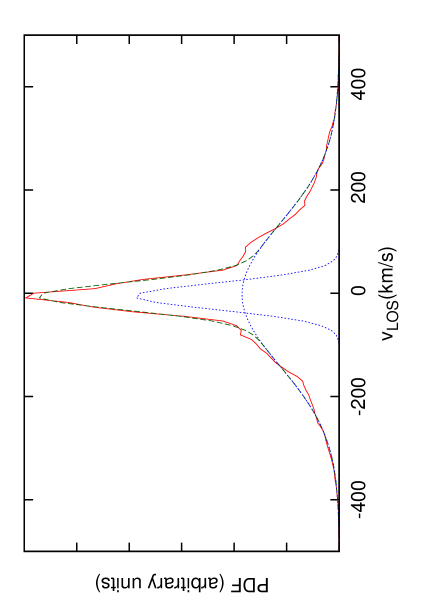
Figure 17: “AGN feedback” cluster: the solid (red) curves are the velocity PDFs from the simulation. The dashed (green) curves are the recovered PDFs from the best-fit models, and the dotted (blue) curves are the individual components. Numerical values of fits are in Table 7.

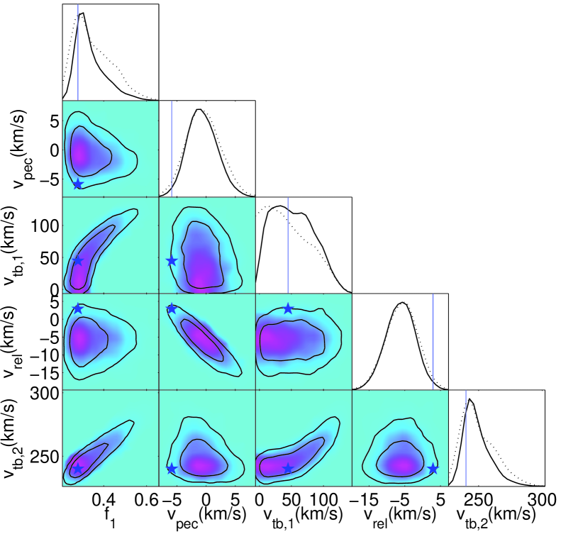
Figure 18: Error contours for the “AGN feedback” case: contours depict the 68%, 95% confidence levels for the marginalized distribution; the shadings shows the mean likelihood of the samples; the solid and dashed curves in the 1-D plots are the fully marginalized posterior and relative mean likelihood of the samples, respectively. The stars and vertical lines label the positions of the true values.

Table 7: “AGN feedback” cluster: best-fit parameters and their uncertainties for the simulated PDF in Fig. 17. The “true values” are obtained by fitting the PDF directly, while the recovered values are obtained from the mock spectrum of $10^{5}$ photons, which includes line blending, thermal broadening, instrument noise, and continuum emission.

	$f_{1}$	$v_{pec}$(km/s)	$v_{rel}$(km/s)	$v_{tb,1}$(km/s)	$v_{tb,2}$(km/s)
True values	$0.28_{-0.01}^{+0.01}$	$-5.89_{-0.84}^{+0.78}$	$2.91_{-1.72}^{+2.16}$	$44.72_{-1.32}^{+1.83}$	$240.07_{-1.89}^{+2.84}$
Recovered	$0.30_{-0.01}^{+0.08}$	$-1.58_{-1.96}^{+2.66}$	$-4.38_{-4.98}^{+2.94}$	$23.43_{-10.56}^{+50.80}$	$246.80_{-3.42}^{+10.89}$

The second example is a FLASH simulation with static gravity and radiative cooling of a cluster with an AGN in the center (hereafter denoted as “AGN feedback”); a simulation snapshot was kindly provided to us by Marcus Brüggen. The simulated cluster, meant to mimic Hydra A, is described in Brüggen et al. (2007) and Simionescu et al. (2009); numerous plots of the velocity field can also be found in Vazza, Roediger & Brueggen (2012). Here, we briefly summarize some properties. The box size was 1 Mpc and AMR resolution reached a peak of 0.5 kpc in the center, and a maximum of (1,4,8) kpc outside (16,100,200) kpc respectively. A bipolar jet 2 kpc in diameter with power $L_{\rm jet}=3\times 10^{45}\,{\rm erg\,s^{-1}}$ was then introduced; for the analyzed snapshot the bulk velocity along the jet is $\sim 1500-1800\,{\rm kms^{-1}}$, and a $M\sim 1.3$ shock has been driven into the surrounding ICM. The AGN was also given a bulk velocity of $\sim 670\,{\rm km\,s^{-1}}$ along the direction of (-1,1,0) relative to the ambient ICM, to mimic the observed offset between the shock center and the AGN in Hydra A. In Fig 16, we show a 1 Mpc size density and velocity field map on the y-z plane through the center. The size of the figure is 1 Mpc. The large bulk velocity along the x-direction has been subtracted from the figure. The outflows from the AGN stir the gas in the central region ($\sim 300$ kpc in radius), while the ambient gas is left relatively quiescent. The velocity field is predominantly radial outside 100 kpc (associated with jet expansion and the running shock), while it is close to isotropic within 100 kpc, indicating that instabilities have efficiently isotropized and distributed the jet power. In Fig. 17, we plot the emission-weighted velocity PDF along the z-direction inside an area of $1\times 1~{}{\rm Mpc}^{2}$. The division between turbulent and quiescent gas shows up in the velocity PDF as a double Gaussian distribution – a narrow Gaussian corresponding to the quiescent gas outside the core, and a broad Gaussian corresponding to the turbulent gas in the center. This is an example of non-volume filling turbulence discussed in § 2.2. Note that we have pessimistically chosen a viewing direction in which there are no bulk motions (similar to the “width driven” case of the preceding example). For other viewing angles, the jet expansion drives bulk motions which result in two clear peaks in the spectrum (similar to the preceding “separation driven” case).

The scales in this Hydra A example are so large that in this particular instance, the velocity structure could be spatially resolved by Astro-H. However, Hydra A is of course an extremely rare and energetic outburst; for more typical jet luminosities of $L_{\rm jet}\sim 10^{44}\,{\rm erg\,s^{-1}}$, the turbulently stirred region will be at least a factor of $\sim 30^{1/3}\sim 3$ smaller or $\sim 100$ kpc in size, and hence barely resolved by Astro-H. In this instance, mixture modeling will still be required to uncover the filling fraction of turbulence. Also, as previously discussed, MHD simulations show that motions are not efficiently isotropized and distributed within the region of influence of the AGN, so in reality there could be small scale intermittency in turbulence which would be spatially unresolved, but detectable with mixture modeling.

To approximate such situations, we analyze the spectrum with the velocity PDF shown in Fig. 17, where the effects of line blending, thermal broadening, instrument noise, and continuum emission have been included. This is a clear example of the “width driven” scenario, with $\sigma_{1}/\sigma_{2}={0.70}$. We were unable to recover the velocity PDF from the mock spectrum with $10^{4}$ photons. The estimated BIC values for the single and double component models using the “true values” indeed show that the single component model is preferred for $10^{4}$ photons ($BIC_{\rm double}-BIC_{\rm single}$=17). However, with $10^{5}$ photons (which is for instance, possible for Perseus; see Table 2), the two components could be easily separated (in this case, $BIC_{\rm double}-BIC_{\rm single}$=-102). The results are given in Table 7. Again, here the “true values” are obtained by fitting the PDF directly, by generating a Monte-Carlo sample of $10^{4}$ photons. The corresponding 2-D error contours and marginalized posterior are shown in Fig. 18. Note the firm lower limit of $\sim 30\%$ to the quiescent component; a clear detection that turbulence is not volume-filling. The velocity dispersion and hence the energy density in the turbulent component are also accurately recovered.

6 Conclusions

Gas motions can have profound influence on many physical processes in the ICM, but thus far we have lacked a direct measurement of turbulence in clusters. Upcoming X-ray missions–in particular Astro-H–are poised to change that, by directly measuring turbulent broadening of spectral lines. Thus far, most work has focussed on how gas motions can alter the mean and width of X-ray emission lines from galaxy clusters. However, the detailed shape of the line profile has valuable information beyond these first two moments. Exploiting the line shape (and thus the high spectral resolution of upcoming missions such as Astro-H) can in many cases ameliorate poor angular resolution in inferring the 3D velocity field. The main point of this paper is that the line-of sight velocity PDF can often be meaningfully decomposed into multiple distinct and physically significant components. The separation is based on deviations of line profiles from a single Gaussian shape, driven by either the difference in width (“width-driven”, WD) or mean (“separation-driven”, SD) of the components. Such a mixture decomposition yields qualitatively different results from a single component fit, and the recovered mixture parameters have physical significance. For instance, bulk flows and sloshing produce components with offset means, while partial volume-filling turbulence from AGN or galaxy stirring leads to components with different widths. The offset between components allows us to measure gas bulk motions and separate them from small-scale turbulence, while component fractions and widths constrain the emission weighted volume and turbulent energy density in each component. With the MCMC algorithm and Fisher matrix techniques, we evaluate the prospects of using Gaussian mixture models to separate and constrain different velocity modes in galaxy clusters from the 6.7 keV Fe line complex. We found that with the $10^{4}$ photons (which is feasible for the $\sim 14$ nearest clusters; see Table 2), the components could be constrained with $\sim 10$% accuracy in WD cases, and $\sim 1$% accuracy in SD cases, in both toy models and simulations of clusters with cold fronts and AGN feedback respectively. Continuum emission degrades the constraints in WD cases, while it has little impact on the SD cases. On the other hand, line blending appear to have little impact. We generally find that Astro-H is effective in separating different components when either the offset between the components or the width of one of the components is larger than $\sim 200$ km/s. Using PDFs taken from numerical simulations as “basis” functions, we find that reasonable deviations from Gaussianity in the mixture components do not affect our results. We also study error scalings and use information criteria to determine when a mixture model is preferred.

Many extensions of this method are possible. For instance: (i) It would be interesting to compare the separation between bulk/turbulent motions obtained from mock X-ray spectra by mixture modeling, with algorithms for performing this separation for the full 3D velocity field in numerical simulations (e.g., Vazza, Roediger & Brueggen (2012)), to see how close the correspondence is. (ii) In this study, we have assumed that due to Astro-H’s poor spatial resolution, only line-of-sight information about the velocity field is possible. In principle, it should be possible also to obtain information about variation of the velocity field in the plane of the sky. For nearby clusters such as Perseus, it should be possible to examine the line shape as a function of projected radial position to obtain a full 3D reconstruction of the velocity field (a more detailed implementation of the suggestion by Zhuravleva et al. (2012) to study the variation of line center and width with projected radial position). It would be very interesting to study the variation of mixture parameters as a function of position in high-resolution simulations. Even for more distant clusters, a coarse-grained tiling of the cluster should be possible. (iii) High resolution X-ray imaging of cold-front clusters yield information about density/temperature contact discontinuities in the plane of the sky. This has already been used infer the presence of sloshing and bulk motions, as well as physical properties of the ICM such as viscosity and thermal conductivity. Combining information about the density/temperature contact discontinuity in the plane of the sky with the line of sight information obtained by mixture modeling could enhance our understanding of gas sloshing in clusters, and give more precise constraints on velocities. It would likewise be interesting to employ mixture modeling on spectra of the violent merger clusters with classic bow shocks.

More generally, mixture modeling of spectra should prove useful whenever there are good reasons to believe that there are multiple components to the thermal or velocity field, and/or the line profile shows significant deviations from Gaussianity. For instance, it might be fruitful to consider applications to the ISM (e.g., Falgarone, Hily–Blant & Pety (2004); Lazarian & Pogosyan (2006)), or Ly$\alpha$ emission from galaxies (e.g., Hansen & Oh (2006); Dijkstra & Hultman Kramer (2012)).

Appendix A Gibbs Sampling MCMC Mixture Models

In this paper, we have adopted a “poor man’s” approach to mixture modeling, in that we have binned the data, and dealt with the log-Poisson likelihood of the binned data. In principle, binning destroys information; however, in practice we have found that given the large number of data points, this information loss is negligible. We chose to adopt this approach since it is simpler and faster (each Monte Carlo simulation now requires operations over $\sim 50$ bins rather than $\sim 10^{4}$ data points; hence it is about $\sim 200$ times faster). In this Appendix, we describe a more statistically rigorous way of Bayesian parameter estimation with mixture models (Roeder & Wasserman, 1997; Gelman et al., 2004; Marin, Mengersen & Robert, 2005; Kelly, 2007), and show how it compares with this simpler method. We use the convention used in statistical literature of “$\sim$” to denote “is distributed as” or “is drawn from”, rather than the usual “is to rough order of magnitude” in astronomical literature.

We will perform MCMC samples of the full posterior distribution of the mixture model. This requires priors to be specified; formally, for Gaussian mixture models, an injudicious choice (such as a uniform prior) can lead to improper (non-integrable) posterior densities (see Roeder & Wasserman (1997) for further discussion of this issue). A particularly convenient choice of priors are conjugate priors, in which the posterior distributions $p(\theta|x)$ are in the same family as the prior probability distribution $p(\theta)$. For instance, the Gaussian family is conjugate to itself (or self-conjugate) with respect to a Gaussian likelihood function: if the likelihood function is Gaussian, choosing a Gaussian prior over the mean will ensure that the posterior distribution is also Gaussian. Fortunately, all members of the exponential family have conjugate priors; for our mixture model, they are (Gelman et al., 2004):

$$(\omega_{1},\ldots,\omega_{k}) \sim {\rm Dir}(a_{1},\ldots,a_{k})$$ (8)

$$\mu_{j} \sim {\cal N}(\tilde{\mu}_{j},\tau_{j}^{2})$$ (9)

$$\sigma_{j}^{2} \sim {\rm Inv-Gamma}(\alpha_{j},\beta_{j}).$$ (10)

These prior distributions in turn require further parameters–known as hyper-parameters–to be specified. In the absence of prior information, techniques exist to allow these hyper-parameters to become additional parameters in the statistical fit, and thus be determined by the data itself (Roeder & Wasserman, 1997). However, given that we do have guidance from both theory and other observations (e.g. X-ray imaging; morphology; temperature and density profiles) about the expect thermal and turbulent broadening of the spectrum, it is reasonable to adopt fixed priors. Here we adopt uninformative priors, but describe the choice of priors in some detail in case more informative priors are desired.

• Mixture weights $\omega_{j}$. The prior for the mixture weights, $(\omega_{1},\ldots,\omega_{k})\sim{\rm Dir}(a_{1},\ldots,a_{k})$ is a Dirichlet distribution, which is conjugate to the multinomial distribution, the following sense: given a prior ${\rm Dir}(a_{1},\ldots,a_{k})$, then if $(b_{1},\ldots,b_{k})$ is the number of occurrences of each event $i$ in a sample of $n$ events, the posterior is ${\rm Dir}({\bf a}+{\bf b})$. If there is no prior information to favor one component over another, then it is common practice to set all members of the prior $a_{i}$ to a common value $a$, known as the concentration parameter; $a\ll 1$ favors concentration amongst a few components, whilst $a\gg 1$ favors almost equal dispersion amongst all components. Here, we adopt a ${\rm Dirichlet}(1,\ldots,1)$ prior, which is equivalent to a uniform prior on ${\bf\omega}$, under the constraint that $\sum_{j=1}^{k}\omega_{j}=1$.

• Line centers $\mu_{j}$. We adopt a normal prior for the line centers, $\mu_{j}\sim{\cal N}(\tilde{\mu}_{j},\tau_{j}^{2})$, where $\tilde{\mu}_{j}$ are the known line centers in the absence of turbulent motions. We set a very weak prior $\tilde{\mu}_{j}=\mu$, where $\mu$ is the mean energy of all photons, and $\tau_{j}=(c_{s}/(\sqrt{3}c)E_{o}$, where $c_{s}/\sqrt{3}$ corresponds to typical line of sight velocities of transonic bulk motions, and $E_{o}$ is the line center energy.

• Line widths $\sigma^{2}_{j}$. The prior is the inverse Gamma distribution, $\sigma_{j}^{2}\sim{\rm Inv-Gamma}(\alpha_{j},\beta_{j})$; the inverse Gamma distribution has the desirable property that it is bounded below at zero, and is defined such that $1/\sigma_{j}^{2}$ obeys a Gamma distribution. Two constraints are needed to determine the two parameters of the distribution, $(\alpha_{j},\beta_{j})$. Since the inverse-Gamma distribution is highly asymmetric, with a long tail to high values of $\sigma_{j}^{2}$, we do not use estimates for the first two moments of the distribution to set $(\alpha_{j},\beta_{j})$. Instead, we set the mode of the distribution to $\sigma_{\rm mode}^{2}=\sigma_{\rm low}^{2}=\beta_{i}/(\alpha_{i}+1)$, where $\sigma_{\rm low}^{2}=\sigma^{2}_{\rm therm}+\sigma^{2}_{\rm instrum}$ is the line width in the absence of turbulence; i.e., due to thermal and instrumental broadening alone. The asymmetric nature of the Inv-Gamma distribution generally implies that $P(\sigma^{2}<\sigma_{\rm mode}^{2})\sim 0.1-0.2$. We require that $P(\sigma^{2}>\sigma_{\rm high}^{2})=0.1$, where $\sigma^{2}_{\rm high}=\sigma^{2}_{\rm low}+v_{\parallel,{\rm max}}^{2}$, and $v_{\parallel,{\rm max}}^{2}$ is such that $U_{\rm turb}\sim 0.5U_{\rm therm}$ for isotropic turbulence. Together, these two requirements allow $\alpha,\beta$ to be determined, and result in $\sim 70-80\%$ of samples drawn from the prior to lie between $\sigma^{2}_{\rm low}$ and $\sigma^{2}_{\rm high}$. This fairly loose prior allows $\sigma^{2}_{j}$ to be mostly driven by the data. A similar procedure can be used for more informative priors.

Our goal is to calculate the posterior of the model parameters, given the prior distribution and the data, and draw samples from this posterior in a numerically tractable manner. Equation (1) in §3 is the probability of drawing a data point with value $x$, given the model parameters $\theta$. Since data points are independent, the likelihood of a data set is the product of the probabilities for each data point:

$${\cal L}(x|\theta)=\prod_{i}f(x_{i}|\theta).$$ (11)

The posterior probability of the model parameters $\theta$, given the data $x$ and priors for the model parameters $p(\theta|\tilde{\theta})$, where $\tilde{\theta}$ are the known hyper-parameters, is then simply:

$$P(\theta|x,\tilde{\theta})\propto{\cal L}(x|\theta)p(\theta|\tilde{\theta}).$$ (12)

In numerical work, we will usually work with the logarithm of the posterior, rather than the posterior itself, to avoid problems with underflow and rounding to zero. However, from equation (1), evaluating the posterior involves the sum of Gaussians, each of which may be so small as to underflow when reconstructed from their logarithms. One must therefore use the log-sum-exp formula (e.g., see Press et al. (2007)):

$${\rm log}\left(\sum_{i}{\rm exp}(z_{i})\right)=z_{\rm max}+{\rm log}\left(\sum_{i}{\rm exp}(z_{i}-z_{\rm max})\right),$$ (13)

where $z_{i}$ are the logarithms of small quantities and $z_{\rm max}$ is their maximum. This guarantees that at least one exponentiation won’t underflow, and any that do could have been neglected anyhow.

We now draw Markov-Chain Monte Carlo (MCMC) samples from the posterior distribution. The Metropolis-Hastings algorithm for drawing MCMC samples is probably the one most familiar to readers; for instance, it is the heart of the widely used software package COSMOMC (Lewis & Bridle, 2002), which we also used previously. Here we use instead Gibbs sampling, which is the most commonly used approach in Bayesian mixture estimate (e.g., Marin, Mengersen & Robert (2005), and references therein); it is in fact a special case of the Metropolis-Hastings algorithm (Gilks, Richardson & Spiegelhalter, 1996), even though historically it was developed separately. In Gibbs sampling, one draws each parameter $\theta_{i}$ from its full conditional distribution, which is obtained by holding all components of $\theta$ constant except for $\theta_{i}$, and sampling from the posterior as a function of $\theta_{i}$ alone. It can be shown that (unlike the Metropolis-Hastings algorithm) the acceptance probability is one in this case, i.e., we can always accept a sample drawn from the conditional distribution $P(\theta_{i}|\theta^{-})$ (where $\theta^{-}$ denotes “values of all parameters except one”). To draw a sample, one simply cycles through each component of $\theta$ in turn. Note that, unlike the Metropolis-Hastings method, each component of $\theta$ gets reset to a value completely independent of its previous value (although $\theta^{-}$ does depend on previous values; thus, we still have a Markov chain). Thus, in principle larger steps in parameter space are possible than with MH sampling, since with the latter, large multi-variate steps will have low acceptance probabilities and almost certainly be rejected. Despite these obvious advantages, a major disadvantage of Gibbs sampling is that it requires the full conditional distribution to be correctly normalized (unlike MH sampling, where an unnormalized posterior is sufficient), and thus the numerically expensive computation of normalizing constants for each $\theta^{-}$ (as well as a practical means of drawing $\theta_{i}$ from each conditional distribution). Fortunately, for Gaussian mixture models, the use of data augmentation and conjugate priors allows for analytic conditional distributions, for which there are well-known random number generators.

We adopt a data augmentation approach to the “missing data” problem previously mentioned: the particular mixture to which a data point belongs is unknown, obviating a straightforward calculation of model parameters. We can treat this unknown membership by assigning to each observation $x_{i}$ a new variable $z_{i}\in{1,2,\ldots,k}$ which indicates which mixture the data point belongs to. Given the augmented membership variable $z_{i}$, equation (1) then reduces to:

$$f(x_{i}|z_{i}=j,\theta)\sim f_{j}(x_{i}|\mu_{j},\sigma^{2}_{j})$$ (14)

where $f_{j}(x|\mu_{j},\sigma^{2}_{j})$ is the $j$th normal mixture component. Of course, we do not know the $z_{i}$, but we know their probability distribution: since the probability that a data point $x_{i}$ belongs to a mixture $j$ is $p_{j}\propto w_{j}f_{j}(x_{i}|\mu_{j},\sigma^{2}_{j})$ (normalized such that $\sum_{j}p_{j}=1$), the $z_{i}$ belong to a multinomial distribution $z_{i}\sim{\cal M}_{j}(1;p_{1},\ldots,p_{k})$.

With this membership variable $z_{i}$ and the conjugate priors in equations (8),(9),(10), we can compute the conditional distributions, which all take the functional form of their conjugate priors. There are well-established algorithms for drawing random numbers from all of these analytic distributions. The mixing fractions $\omega$ are Dirichlet distributed:

$$(\omega_{1},\ldots,\omega_{k})\sim{\rm Dir}(a_{1}+n_{1},\ldots,a_{k}+n_{k})$$ (15)

where $n_{j}$ are the number of data points in mixture $j$, obtained by summing over the indicator variables $z_{i}$. We can immediately see that the hyper-parameters we have chosen $a_{1},\ldots,a_{k}=1$ will have little influence for a large sample. The means $\mu_{j}$ are Gaussian distributed:

$$\mu_{j}\sim{\cal N}\left(\frac{\frac{\tilde{\mu}_{j}}{\tau_{j}^{2}}+\frac{\sum_{i|z_{i}=j}x_{i}}{\sigma_{j}^{2}}}{\frac{n_{j}}{\sigma_{j}^{2}}+\frac{1}{\tau_{j}^{2}}},\left(\frac{n_{j}}{\sigma_{j}^{2}}+\frac{1}{\tau_{j}^{2}}\right)^{-1}\right)$$ (16)

where the sum runs over all data points $x_{i}$ which belong to mixture $j$, as indicated by the membership variable $z_{i}=j$. The variances are drawn from an inverse-Gamma distribution:

$$\sigma^{2}_{j}\sim{\rm Inv-Gamma}\left(\alpha_{j}+\frac{n_{j}}{2},\beta_{j}+\frac{1}{2}\sum_{i|z_{i}=j}(x_{i}-\mu_{j})^{2}\right).$$ (17)

Finally, at every iteration we have to draw a new set of indicator variables $z_{i}$ from a multinomial distribution:

$$z_{i}\sim{\cal M}(1;p_{1},\ldots,p_{k})$$ (18)

and $p_{j}(x_{i})\propto w_{j}f_{j}(x_{i}|\mu_{j},\sigma^{2}_{j})$ (normalized such that $\sum_{j}p_{j}=1$). A set of each of these random draws then comprises a single Monte-Carlo sample from the posterior distribution. In our calculations, we find that computing time is heavily dominated by random draws from the multinomial random number generator. We therefore parallelized the multinomial random number generator, and found that this allowed a significant (close to linear) reduction in computation time.

As before, we deal with the “label-switching” problem by demanding that $\mu_{1}<\mu_{2}$. Note that this is still an area of active research (e.g., see Jasra, Holmes & Stephens (2005)); as yet there is no consensus solution in the statistical community. Alternatively, we find that if we enforce asymmetric priors, this is usually sufficient to break the symmetry in the modes of the posterior and single out a single one.

We have experimented with running this Gibbs sampling MCMC and the Cash-C Metropolis-Hastings MCMC described in the text, and found that they give similar results. For instance, it gives almost exactly the same results for the single line SD case given in Table 4, and similar results for the WD case given in Table 3. Interestingly, often the trace plots of the Gibbs sampling MCMC method for the WD case show that it has somewhat poorer mixing and convergence properties—indicating that it is more badly affected by parameter degeneracies. The greater robustness of the method we used in this paper stems from the use of covariance matrix information to improve the proposal distribution in COSMOMC (Lewis & Bridle, 2002); a similar means of orthogonalizing parameters should be implemented here to ensure robustness. Overall, there is no reason to use full mixture modeling for the purposes of this paper. However, the algorithm described in this Appendix should be preferred when there are fewer data points, and binning is deprecated.

References

- Akaike (1974) Akaike H., 1974, IEEE Transactions on Automatic Control, 19, 716
- Ashman, Bird & Zepf (1994) Ashman K. M., Bird C. M., Zepf S. E., 1994, AJ, 108, 2348
- Balbus & Soker (1990) Balbus S. A., Soker N., 1990, ApJ, 357, 353
- Battaglia et al. (2011a) Battaglia N., Bond J. R., Pfrommer C., Sievers J. L., 2011a, ArXiv e-prints
- Battaglia et al. (2011b) —, 2011b, ArXiv e-prints
- Birzan et al. (2004) Birzan L., Rafferty D. A., McNamara B. R., Wise M. W., Nulsen P. E. J., 2004, ApJ, 607, 800
- Brüggen et al. (2007) Brüggen M., Heinz S., Roediger E., Ruszkowski M., Simionescu A., 2007, MNRAS, 380, L67
- Brüggen, Hoeft & Ruszkowski (2005) Brüggen M., Hoeft M., Ruszkowski M., 2005, ApJ, 628, 153
- Brunetti & Lazarian (2007) Brunetti G., Lazarian A., 2007, MNRAS, 378, 245
- Brunetti et al. (2001) Brunetti G., Setti G., Feretti L., Giovannini G., 2001, MNRAS, 320, 365
- Bryan (1999) Bryan G. L., 1999, Comput. Sci. Eng., 1, 46
- Cash (1979) Cash W., 1979, ApJ, 228, 939
- Celeux, Hurn & Robert (2000) Celeux G., Hurn M., Robert C., 2000, Journal of the American Statistical Association, 957
- Chen et al. (2007) Chen Y., Reiprich T. H., Böhringer H., Ikebe Y., Zhang Y.-Y., 2007, aap, 466, 805
- Chepurnov & Lazarian (2006) Chepurnov A., Lazarian A., 2006, ApJ, 693, 1074
- Cho et al. (2003) Cho J., Lazarian A., Honein A., Knaepen B., Kassinos S., Moin P., 2003, ApJL, 589, L77
- Cho et al. (2009) Cho J., Vishniac E. T., Beresnyak A., Lazarian A., Ryu D., 2009, ApJ, 693, 1449
- Churazov et al. (2004) Churazov E., Forman W., Jones C., Sunyaev R., Böhringer H., 2004, MNRAS, 347, 29
- Churazov et al. (2008) Churazov E., Forman W., Vikhlinin A., Tremaine S., Gerhard O., Jones C., 2008, MNRAS, 388, 1062
- Churazov et al. (2010) Churazov E. et al., 2010, MNRAS, 404, 1165
- Dempster, Laird & Rubin (1977) Dempster A., Laird N., Rubin D., 1977, Journal of the Royal Statistical Society. Series B (Methodological), 39, 1
- Dennis & Chandran (2005) Dennis T. J., Chandran B. D. G., 2005, ApJ, 622, 205
- Dijkstra & Hultman Kramer (2012) Dijkstra M., Hultman Kramer R., 2012, ArXiv e-prints
- Dunn, Fabian & Sanders (2006) Dunn R. J. H., Fabian A. C., Sanders J. S., 2006, MNRAS, 366, 758
- Dursi & Pfrommer (2008) Dursi L. J., Pfrommer C., 2008, ApJ, 677, 993
- Enßlin & Vogt (2006) Enßlin T. A., Vogt C., 2006, A&A, 453, 447
- Fabian et al. (2003) Fabian A. C., Sanders J. S., Allen S. W., Crawford C. S., Iwasawa K., Johnstone R. M., Schmidt R. W., Taylor G. B., 2003, MNRAS, 344, L43
- Falgarone, Hily–Blant & Pety (2004) Falgarone E., Hily–Blant P., Pety J., 2004, in Astronomical Society of the Pacific Conference Series, Vol. 323, Star Formation in the Interstellar Medium: In Honor of David Hollenbach, D. Johnstone, F. C. Adams, D. N. C. Lin, D. A. Neufeeld, & E. C. Ostriker , ed., p. 185
- Gaspari et al. (2011) Gaspari M., Melioli C., Brighenti F., D’Ercole A., 2011, MNRAS, 411, 349
- Gelman et al. (2004) Gelman A., Carlin J., Stern H., Rubin D., 2004, Bayesian data analysis. CRC press
- Gilks, Richardson & Spiegelhalter (1996) Gilks W., Richardson S., Spiegelhalter D., 1996, Markov chain Monte Carlo in practice. Chapman & Hall/CRC
- Guglielmetti, Fischer & Dose (2009) Guglielmetti F., Fischer R., Dose V., 2009, MNRAS, 396, 165
- Hansen & Oh (2006) Hansen M., Oh S. P., 2006, MNRAS, 367, 979
- Heinz, Brüggen & Morsony (2010) Heinz S., Brüggen M., Morsony B., 2010, ApJ, 708, 462
- Heinz et al. (2006) Heinz S., Brüggen M., Young A., Levesque E., 2006, MNRAS, 373, L65
- Iapichino & Niemeyer (2008) Iapichino L., Niemeyer J. C., 2008, MNRAS, 388, 1089
- Inogamov & Sunyaev (2003) Inogamov N. a., Sunyaev R. a., 2003, Astronomy Letters, 29, 791
- Jasra, Holmes & Stephens (2005) Jasra A., Holmes C., Stephens D., 2005, Statistical Science, 50
- Jeffreys (1961) Jeffreys H., 1961, Theory of Probability. Oxford University Press
- Kelly (2007) Kelly B. C., 2007, ApJ, 665, 1489
- Kelly, Fan & Vestergaard (2008) Kelly B. C., Fan X., Vestergaard M., 2008, ApJ, 682, 874
- Kim (2007) Kim W., 2007, ApJL, 667, L5
- Kim & Narayan (2003) Kim W.-T., Narayan R., 2003, ApJ, 596, 889
- King & Pringle (2007) King A. R., Pringle J. E., 2007, MNRAS, 377, L25
- Komatsu et al. (2011) Komatsu E. et al., 2011, ApJS, 192, 18
- Kunz et al. (2011) Kunz M. W., Schekochihin A. A., Cowley S. C., Binney J. J., Sanders J. S., 2011, MNRAS, 410, 2446
- Lau, Kravtsov & Nagai (2009) Lau E. T., Kravtsov A. V., Nagai D., 2009, ApJ, 705, 1129
- Lau, Kravtsov & Nagai (2009) Lau E. T., Kravtsov A. V., Nagai D., 2009, ApJ, 705, 11
- Lau et al. (2011) Lau E. T., Nagai D., Kravtsov A. V., Zentner A. R., 2011, ApJ, 734, 93
- Lazarian & Pogosyan (2000) Lazarian A., Pogosyan D., 2000, ApJ, 537, 720
- Lazarian & Pogosyan (2006) —, 2006, ApJ, 652, 1348
- Lewis & Bridle (2002) Lewis A., Bridle S., 2002, Physical Review D, 66
- Liddle (2004) Liddle A. R., 2004, MNRAS, 351, L49
- Mackay (2003) Mackay D. J. C., 2003, Information Theory, Inference and Learning Algorithms. Cambridge Univ Press
- Marin, Mengersen & Robert (2005) Marin J., Mengersen K., Robert C., 2005, Handbook of Statistics, 25, 459
- Markevitch & Vikhlinin (2007) Markevitch M., Vikhlinin A., 2007, Physics Reports, 443, 1
- Markevitch & Vikhlinin (2007) Markevitch M., Vikhlinin A., 2007, Physics Reports, 443, 1
- McNamara & Nulsen (2007) McNamara B. R., Nulsen P. E. J., 2007, ARA&A, 45, 117
- McNamara & Nulsen (2012) —, 2012, ArXiv e-prints
- Morsony et al. (2010) Morsony B. J., Heinz S., Brüggen M., Ruszkowski M., 2010, MNRAS, 407, 1277
- Mukherjee et al. (1998) Mukherjee S., Feigelson E. D., Jogesh Babu G., Murtagh F., Fraley C., Raftery A., 1998, ApJ, 508, 314
- Muratov & Gnedin (2010) Muratov A. L., Gnedin O. Y., 2010, ApJ, 718, 1266
- Norman & Bryan (1999) Norman M. L., Bryan G. L., 1999, in Miyama S. M., Tomisaka K., Hanawa K., eds, Astrophys. Space Sci. Library, Vol. 240, Numerical Astrophysics. Kluwer, Boston, p. 19
- O’Neill, DeYoung & Jones (2009) O’Neill S. M., DeYoung D. S., Jones T. W., 2009, ApJ, 694, 1317
- O’Neill & Jones (2010) O’Neill S. M., Jones T. W., 2010, ApJ, 710, 180
- O’Shea et al. (2004) O’Shea B. W., Bryan G., Bordner J., Norman M. L., Abel T., Harkness R., Kritsuk A., 2004, in Plewa T., Linde T., Weirs G., eds, Adaptive Mesh Refinement: Theory and Applications. Berlin, Springer, p. 343
- Parrish et al. (2012) Parrish I. J., McCourt M., Quataert E., Sharma P., 2012, MNRAS, 419, L29
- Parrish, Quataert & Sharma (2010) Parrish I. J., Quataert E., Sharma P., 2010, ApJL, 712, L194
- Porter et al. (2010) Porter F. S. et al., 2010, in Society of Photo-Optical Instrumentation Engineers (SPIE) Conference Series, Vol. 7732, Society of Photo-Optical Instrumentation Engineers (SPIE) Conference Series
- Press et al. (2007) Press W., Flannery B., Teukolsky S., Vetterling W., 2007, Numerical Recipes. Cambridge Univ Press
- Rebusco et al. (2005) Rebusco P., Churazov E., Böhringer H., Forman W., 2005, MNRAS, 359, 1041
- Rebusco et al. (2008) Rebusco P., Churazov E., Sunyaev R., Böhringer H., Forman W., 2008, MNRAS, 384, 1511
- Reynolds, Brenneman & Stocke (2005) Reynolds C. S., Brenneman L. W., Stocke J. T., 2005, MNRAS, 357, 381
- Roeder & Wasserman (1997) Roeder K., Wasserman L., 1997, Journal of the American Statistical Association, 92, 894
- Ruszkowski et al. (2007) Ruszkowski M., Enßlin T. A., Brüggen M., Heinz S., Pfrommer C., 2007, MNRAS, 378, 662
- Ruszkowski et al. (2011) Ruszkowski M., Lee D., Brüggen M., Parrish I., Oh S. P., 2011, ApJ, 740, 81
- Ruszkowski & Oh (2010) Ruszkowski M., Oh S. P., 2010, ApJ, 713, 1332
- Ruszkowski & Oh (2011) —, 2011, MNRAS, 414, 1493
- Ryu et al. (2008) Ryu D., Kang H., Cho J., Das S., 2008, Science, 320, 909
- Sanders, Fabian & Smith (2011) Sanders J. S., Fabian A. C., Smith R. K., 2011, MNRAS, 410, 1797
- Sanders et al. (2010) Sanders J. S., Fabian A. C., Smith R. K., Peterson J. R., 2010, MNRAS, 402, L11
- Schuecker et al. (2004) Schuecker P., Finoguenov A., Miniati F., Böhringer H., Briel U. G., 2004, A&A, 426, 387
- Schwarz (1978) Schwarz G., 1978, Ann. Statist., 5, 461
- Shaw et al. (2010) Shaw L. D., Nagai D., Bhattacharya S., Lau E. T., 2010, ApJ, 725, 1452
- Shin, Sekora & Byun (2009) Shin M.-S., Sekora M., Byun Y.-I., 2009, MNRAS, 400, 1897
- Simionescu et al. (2009) Simionescu A., Roediger E., Nulsen P. E. J., Brüggen M., Forman W. R., Böhringer H., Werner N., Finoguenov A., 2009, A&A, 495, 721
- Simionescu et al. (2008) Simionescu A., Werner N., Finoguenov A., Böhringer H., Brüggen M., 2008, A&A, 482, 97
- Subramanian, Shukurov & Haugen (2006) Subramanian K., Shukurov A., Haugen N. E. L., 2006, MNRAS, 366, 1437
- Sunyaev, Norman & Bryan (2003) Sunyaev R. A., Norman M. L., Bryan G. L., 2003, Astronomy Letters, 29, 783
- Tegmark, Taylor & Heavens (1997) Tegmark M., Taylor A. N., Heavens A. F., 1997, ApJ, 480, 22
- Vazza et al. (2010) Vazza F., Brunetti G., Gheller C., Brunino R., 2010, New Astronomy, 15, 695
- Vazza et al. (2011) Vazza F., Brunetti G., Gheller C., Brunino R., Brüggen M., 2011, A&A, 529, A17+
- Vazza et al. (2009) Vazza F., Brunetti G., Kritsuk A., Wagner R., Gheller C., Norman M., 2009, A&A, 504, 33
- Vazza et al. (2009) Vazza F., Brunetti G., Kritsuk A., Wagner R., Gheller C., Norman M., 2009, aap, 504, 33
- Vazza, Roediger & Brueggen (2012) Vazza F., Roediger E., Brueggen M., 2012, ArXiv e-prints
- Vogt & Enßlin (2005) Vogt C., Enßlin T. A., 2005, A&A, 434, 67
- Werner et al. (2010) Werner N. et al., 2010, ArXiv e-prints
- Zhang et al. (2008) Zhang Y.-Y., Finoguenov A., Böhringer H., Kneib J.-P., Smith G. P., Kneissl R., Okabe N., Dahle H., 2008, aap, 482, 451
- Zhuravleva et al. (2012) Zhuravleva I., Churazov E., Kravtsov A., Sunyaev R., 2012, ArXiv e-prints
- ZuHone, Markevitch & Johnson (2010) ZuHone J. A., Markevitch M., Johnson R. E., 2010, ApJ, 717, 908