Wall-liquid and wall-crystal interfacial free energies via thermodynamic integration: A molecular dynamics simulation study

Abstract

A method is proposed to compute the interfacial free energy of a Lennard-Jones system in contact with a structured wall by molecular dynamics simulation. Both the bulk liquid and bulk face-centered-cubic crystal phase along the (111) orientation are considered. Our approach is based on a thermodynamic integration scheme where first the bulk Lennard-Jones system is reversibly transformed to a state where it interacts with a structureless flat wall. In a second step, the flat structureless wall is reversibly transformed into an atomistic wall with crystalline structure. The dependence of the interfacial free energy on various parameters such as the wall potential, the density and orientation of the wall is investigated. The conditions are indicated under which a Lennard-Jones crystal partially wets a flat wall.

I Introduction

Knowledge of the interfacial free energy between a crystal or liquid in contact with a solid wall is crucial to the understanding of heterogeneous nucleation and wetting phenomena gibbs57 ; adamson97 ; dietrich88 ; rowlinson82 ; degennes85 . However, interfacial free energies are hardly accessible in experiments and in fact only a few measurements have been reported so far (see e.g. adamson97 ; navascues79 ; howe97 ).

Due to the lack of experimental data, particle-based simulation techniques such as Molecular Dynamics (MD) and Monte Carlo (MC) allen-tildesley87 ; landau-binder00 are of special importance to understand the properties of wall-liquid and wall-crystal interfaces and to rationalize calculations in the framework of density functional theory loewen94evans90 ; barker76 ; velasco89 . In this context, MC and MD simulations have been used to understand the microscopic mechanism of fluid wetting on solid surfaces navascues79 ; henderson84 ; miguel06 ; nijmeijer90 ; tang95 as well as the wetting and drying transition of a fluid at liquid-vapor coexistence and in contact with a solid wall nijmeijer90 ; tang95 ; vanleeuwen90 ; bruin91 . The question of how the wall structure affects the interfacial tension with respect to liquid, vapor and solid phases has been also addressed tang95 ; leroy09 .

On a macroscopic scale, a crystal that partially wets a wall might be described as a spherical cap. Then, the contact angle $\theta_{c}$ of the cap with the wall is given by Young’s equation degennes85 ,

$$\gamma_{\text{wc}}+\gamma_{\text{cl}}\cos\theta_{\text{c}}=\gamma_{\text{wl}}\,$$ (1)

with $\gamma_{\text{wc}}$ the wall-crystal, $\gamma_{\text{cl}}$ the crystal-liquid, and $\gamma_{\text{wl}}$ the wall-liquid interfacial free energy. Equation (1) describes the condition of a spherical crystal droplet resting on a wall, being in coexistence with the liquid phase. Incomplete wetting corresponds to contact angles $0<\theta_{c}<\pi$.

On a nanoscopic scale, deviations from Young’s equation can be expected, e.g. due to the contribution of line tension effects gibbs57 ; degennes85 ; weijs11 . To quantify the latter deviations, reliable estimates of $\gamma_{\text{wc}}$, $\gamma_{\text{cl}}$ and $\gamma_{\text{wl}}$ are required. Then, the contact angle can be obtained via Eq. (1) and compared to a direct measurement of $\theta_{c}$.

In this paper, we propose a thermodynamic integration (TI) frenkel-smit02 scheme for the calculation of $\gamma_{\text{wc}}$ and $\gamma_{\text{wl}}$. To obtain $\gamma_{\text{wl}}$, most previous studies have used the mechanical approach of calculating the normal and tangential pressure components at the wall and integrating over the pressure anisotropy (PA) navascues79 ; henderson84 ; nijmeijer90 ; tang95 ; vanleeuwen90 . While the PA method is valid for planar wall-liquid or liquid-vapor interfaces it fails in case of small liquid drops in contact with a solid wall sampayao10 . Moreover, its use is justified only for systems where the interfacial tension equals the interfacial free energy tiller91 . This is true for a wall represented by a time-independent external field henderson84 ; varnik00 ; varnik-thesis00 or a wall made of particles rigidly fixed at the sites of an ideal lattice nijmeijer90 ; tang95 ; vanleeuwen90 ; bruin91 ; bakker89 ; crevecoeur95 . However, for systems which can support stress, such as a wall consisting of a “fully interacting solid phase” laird10 , this method is invalid. For the same reason, the PA technique cannot be used to determine $\gamma_{\text{wc}}$ tiller91 . Even for wall-liquid interfaces, the PA method can yield results with acceptable precision only with huge computational effort. Most previous works based on the PA technique yielded results of low accuracy and the values of the interfacial tension reported in the literature differ widely, even for simple systems.

Due to the obvious disadvantage in using the PA method, a few thermodynamic approaches have been developed to evaluate the wall-liquid and wall-crystal interfacial free energies with improved precision. Heni and Löwen heni99 combined MC simulations and thermodynamic integration to determine the interfacial free energies of hard sphere liquids and solids near a planar structureless wall over a whole range of bulk densities including the solid-liquid coexistence density. In their thermodynamic integration scheme, a bulk hard sphere system was reversibly transformed into a system interacting with a more and more impenetrable wall and finally a hard wall. Fortini and Djikstra fort-djik06 used a thermodynamic integration scheme based on exponential potentials to calculate $\gamma_{\text{wl}}$ and $\gamma_{\text{wc}}$ at bulk coexistence conditions. Their results were in good agreement with those of Heni and Löwen but obtained with significantly higher precision. Due to precrystallization of the hard spheres near the wall close to the bulk freezing transition, both Heni and Löwen and Fortini and Dijkstra extrapolated the value of the interfacial tensions at coexistence from the data at lower densities.

Laird and Davidchack laird07 developed a TI method by the use of “cleaving potentials”, to obtain $\gamma_{\text{wl}}$ and $\gamma_{\text{wc}}$ for hard sphere systems at coexistence. In another work laird10 , they used the “Gibbs-Cahn integration” method, to obtain wall-fluid interfacial free energies for hard sphere systems. This method yielded results consistent with the TI method with “cleaving potentials” but were obtained with significantly less computational effort. However, “Gibbs-Cahn integration” requires that one knows already the interfacial free energy at one point. Deb et al. deb10 ; deb11 compared different methods to obtain wall-fluid and wall-crystal interfacial free energies for hard sphere systems confined by hard walls or, soft walls described by the Weeks-Chandler-Anderson (WCA) potential. They introduced a scheme similar to Wang-Landau sampling wang01 , known as the “ensemble mixing” method, to perform a TI from a system without walls to a system confined by walls. For hard spheres, Deb et al. obtained good agreement with the results of Laird and Davidchack.

In contrast to these few works on hard-sphere systems, there is a dearth of results on the interfacial free energies of systems with continuous potentials, such as Lennard-Jones (LJ) systems. Recently, Leroy et al. leroy09 obtained $\gamma_{\text{wl}}$ for a LJ liquid in contact with a flexible LJ structured wall by the use of a TI technique, known as the “phantom wall” method. In this approach, the structured wall interacting with the liquid is gradually moved away from the liquid, while a structureless flat wall is moved towards it such that in the final state, the liquid interacts only with the structureless wall. Computing the free energy difference during this transformation, along with the interfacial free energy of liquid in contact with the structureless wall, gives $\gamma_{\text{wl}}$. $\gamma_{\text{wl}}$ for the liquid-flat wall system, which serves as the reference state for their system was obtained using the PA technique. Since the PA technique fails in case of crystal-wall interfaces tiller91 one cannot use their scheme to determine $\gamma_{\text{wc}}$ for crystal in contact with a structured wall. In fact, much less is known about $\gamma_{\text{wc}}$ for LJ systems in contact with a wall.

Grochola et al. grochola02ab0405ab developed another TI technique which they have called “$\lambda$-integration”, to determine the surface free energies of solids. In principle, this technique could be also applied to wall-crystal or wall-liquid interfaces, but the method has not been worked out yet for such interfaces.

A straightforward and comprehensive method is thus needed to compute the interfacial free energies of LJ systems in contact with a wall. In the present work, a novel TI scheme is introduced to compute the interfacial free energy of a LJ system confined between walls. We consider both the liquid as well as the fcc crystal phase along the (111) orientation near the wall. While most previous works employing TI methods to obtain $\gamma_{\text{wl}}$ or $\gamma_{\text{wc}}$ are limited to structureless walls, here we specifically consider the case of a structured wall, consisting of particles rigidly attached to the sites of an ideal fcc lattice. Our scheme consists of TI in two steps, providing a reversible thermodynamic path that transforms the bulk LJ system into a LJ fluid or crystal interacting with a structured wall. In the first step, a thermodynamic path is devised to reversibly transform the bulk LJ system without walls and periodic boundary conditions in all directions to a state where it interacts with the structureless wall. This is accomplished by gradually modifying the interaction potential between the wall and the LJ particles along the thermodynamic path. The technique is inspired by the method proposed by Heni and Löwen heni99 to compute the interfacial free energy of hard sphere fluids and crystals in contact with a hard wall.

The LJ system interacting with the flat wall serves as the reference state to calculate the interfacial free energy of the LJ liquid or crystal in contact with a structured wall. In the second step, another TI scheme reversibly changes the structureless wall interacting with the LJ system into a structured wall. This is done by gradually switching off the flat walls and simultaneously switching on the structured walls. While previous methods based on TI techniques for the calculation of $\gamma_{\rm wl}$ make use of “cleaving potentials” laird07 or “phantom walls ” leroy09 , here we directly modify the interaction potential to make the transformation from the reference state to the final state in each of the two steps. Though this TI scheme is specifically developed for a LJ potential, it can be easily generalized to more complex potentials.

The wetting behavior of a liquid or crystal in contact with a structured solid wall will be affected by various parameters. In this work we focus on three parameters: i) the interaction strength between the wall and the LJ system, ii) the density of the structured wall, and iii) the orientation of the structured wall with respect to the interface normal. For these cases, wall-crystal interfacial free energies only for the (111) orientation of the crystal are considered.

Since the PA method has been widely applied in the past to evaluate the wall-liquid interfacial free energy, we will compare results obtained from it with those yielded by the TI method for both flat and structured walls. In addition, we will also show that the interfacial free energies of the LJ system interacting with a flat wall can be obtained directly at coexistence, without any extrapolation from data at low densities, enabling us to investigate its wetting behavior.

Furthermore, to compare the estimates of interfacial free energy yielded by our TI scheme with that obtained in previous works, we apply our technique to a model system studied by Tang and Harris (TH) tang95 using the mechanical definition of the interfacial free energy. Their system consisted of a LJ fluid confined between identical rigid structured walls oriented along the (100) orientation, under conditions of liquid-vapor coexistence. Later, Grzelak and Errington (GE) grzelak08 investigated the same system using Grand Canonical Transition Matrix Monte Carlo (GCTMMC) simulations. They computed the interfacial free energy profile as a function of the surface density at bulk liquid-vapor saturation condition, to obtain the contact angle and the solid-vapor and solid-liquid interfacial tensions. For this system, we will examine the variation of $\gamma_{\rm wl}$ as a function of the wall-liquid interaction strength and compare estimates of $\gamma_{\rm wl}$ from these two studies. Due to the paucity of studies on the crystal-wall interfacial free energy, we will restrict this comparison with previous works only to the wall-liquid interfacial free energy.

In the following, we introduce the details of the model potentials considered in this work (Sec. II), give the various definitions of interfacial free energies, outline the PA method, describe the proposed TI scheme, and provide the main details of the simulation (Sec. III). Then, we present the results (Sec. IV) and finally draw some conclusions (Sec. V).

II Model Potential

The MD system to determine the interfacial excess free energy of a LJ system in contact with a structured wall consists of $N$ identical particles interacting with each other and with the structured wall via a shifted-force LJ allen-tildesley87 potential. If two particles $i$ and $j$ of types $\alpha$ and $\beta$ are separated by a distance $r_{ij}$, the interaction potential is written as

$$u_{\alpha\beta}({r_{\text{ij}}})=\begin{cases}\phi_{\alpha\beta}(r_{ij})-\phi_{\alpha\beta}(r^{\text{c}})-\phi_{\alpha\beta}^{\prime}(r_{ij}=r^{c})[r_{ij}-r^{\text{c}}]\\ \qquad\qquad\text{for $0<r_{ij}\leq r^{\text{c}}$},\\ 0\qquad\qquad\text{for $r_{ij}>r^{\text{c}}$},\end{cases}$$ (2)

where the prime in $\phi_{\alpha\beta}^{\prime}$ denotes the derivative with respect to $r$ and

$$\phi_{\alpha\beta}(r_{ij})=4\epsilon_{\alpha\beta}\left[\left(\frac{\sigma_{\alpha\beta}}{r_{ij}}\right)^{12}-\left(\frac{\sigma_{\alpha\beta}}{r_{ij}}\right)^{6}\right].$$ (3)

In Eq. (2), $\alpha$ or $\beta$ can represent a LJ particle (p) or a structured wall particle (w). The parameters $\epsilon_{\alpha\beta}$ and $\sigma_{\alpha\beta}$ have units of energy and length, respectively. The cut-off distance is set to $r^{c}=2.5\sigma_{\alpha\beta}$.

In the following, energies, lengths and masses are given in units of $\epsilon_{\text{pp}}$, $\sigma_{\text{pp}}$ and $m_{\text{p}}$, respectively. Thus, temperature, pressure and interfacial free energy are expressed in units of $\epsilon_{\text{pp}}/k_{B}$, $\epsilon_{\text{pp}}/\sigma_{\text{pp}}^{3}$ and $\epsilon_{\text{pp}}/\sigma_{\text{pp}}^{2}$, respectively. Time is made dimensionless by reducing it with respect to the characteristic time scale $\sqrt{m_{\text{p}}\sigma_{\text{pp}}^{2}/\epsilon_{\text{pp}}}$. For simplicity, we choose $\sigma_{\rm wp}=\sigma_{\rm pp}$.

The $N$ identical liquid or crystal particles are enclosed within a simulation box of size $L_{\text{x}}\times L_{\text{y}}\times L_{\text{z}}$, using periodic boundary conditions in the $x$ and $y$ directions. In the $z$ direction the particles are confined by the structured wall, between $z=z_{\text{b}}$ at the top and $z=z_{\text{t}}$ at the bottom. The system thus consists of two planar wall-liquid (or wall-crystal) interfaces with a total area of $A=2L_{\text{x}}L_{\text{y}}$. The structured wall is arranged in a manner such that the wall layers closest to the LJ system are positioned at $z_{\text{b}}=-L_{\text{z}}/2$ and $z_{\text{t}}=L_{\text{z}}/2$. Also, an integer number of unit cells was chosen for the structured wall such that the wall is exactly adapted to the lateral size of the simulation cell.

The width of the structured wall is chosen large enough to avoid LJ particles on opposite sides of the wall from interacting with each other since the determination of interfacial free energy by TI or PA methods is built on the assumption of two independent wall-liquid (or wall-crystal) interfaces.

The TI scheme adopted in this work consists of two steps. First, a bulk LJ system with periodic boundary conditions is transformed into a state where the LJ system interacts with impenetrable flat walls. Then, in the second step, the flat walls are reversibly transformed into structured walls. The structureless flat wall (fw) is taken to be a purely repulsive potential interacting along the $z$ direction with the LJ particles and is described by a WCA potential,

$$u_{\text{fw}}(z)=\begin{cases}4\epsilon_{w}\left[\left(\frac{\sigma_{\text{pp}}}{z}\right)^{12}-\left(\frac{\sigma_{\text{pp}}}{z}\right)^{6}+\frac{1}{4}\right]\times w(z)\\ \qquad\text{for $0<z\leq z_{\text{cw}}$},\\ 0\qquad\text{for $z>z_{\text{cw}}$}\end{cases}$$ (4)

with the cut-off $z_{\text{cw}}=2^{1/6}\sigma_{pp}$ and $z=z_{i}-Z$ the distance of particle $i$ at $z_{i}$ to one of the flat walls at $Z=z_{\rm b}$ or $Z=z_{\rm t}$. The function $w(z)$ ensures that $u_{\text{fw}}(z)$ goes smoothly to zero at $z=z_{\text{cw}}$ and is given by

$$w(z)=\frac{1}{h^{4}+\left(1/(z-z_{\text{cw}})^{4}\right)},$$ (5)

where the dimensionless parameter $h$ is set to $0.005$.

To compare to the results of Tang and Harris tang95 and Grzelak and Errington grzelak08 , we also consider a truncated and shifted LJ potential for the particle-particle (pp) and particle-structured wall (pw) interactions,

$$u_{\alpha\beta}^{\ast}(r_{\text{ij}})=\begin{cases}\phi_{\alpha\beta}(r_{ij})-\phi_{\alpha\beta}(r^{c})\qquad\text{for $r_{ij}<r^{c}$},\\ 0\qquad\qquad\qquad\qquad\quad\hskip 6.40204pt\text{for $r_{ij}\geq r^{c}$}\end{cases}$$ (6)

with $\alpha\beta={\rm pp,pw}$ and the cut-off radius $r^{c}=2.5\sigma_{\text{pp}}$. Moreover, we choose $\sigma_{\text{pw}}=1.1\sigma_{\text{pp}}$ and vary the parameter $\epsilon_{\rm pw}$ in units of $\epsilon_{\rm pp}$ in order to determine the interfacial free energy $\gamma_{\rm wl}$ as a function of the strength of the pw interactions. As Tang and Harris tang95 , we use a substrate consisting of three layers of atoms rigidly fixed to fcc lattice sites, with the (100) orientation of the wall facing the liquid along the $z$ direction. The average number density of the liquid is set to $\rho_{\text{p}}=0.661\;\sigma_{\rm pp}^{-3}$ and that of the substrate to $\rho_{\text{w}}=0.59\;\sigma_{\rm pp}^{-3}$ keeping the temperature of the system fixed at $T=0.9k_{\text{B}}/\epsilon_{\text{pp}}$.

III Calculation of interfacial free energies

III.1 Definitions

The Hamiltonian of our model, corresponding to the LJ system interacting with a solid wall, can be written as

$$\begin{split}H({\bf r},{\bf p})=\sum_{i=1}^{N_{\text{p}}}\frac{1}{2m_{i}}{{\bf p}_{i}^{2}}+\sum_{i=1}^{N_{\text{p}}}\sum_{j=i+1}^{N_{p}}u_{\text{pp}}({r_{ij}})+U_{\text{wall}}\end{split}$$ (7)

with $N_{\text{p}}$ the total number of LJ particles and $U_{\text{wall}}$ the wall-particle potential. For interactions of the LJ system with a flat wall, $U_{\text{wall}}=\sum_{i=1}^{N_{\text{p}}}u_{\text{fw}}(z=z_{i}-Z)$, and for the system in contact with a structured wall, $U_{\text{wall}}=\sum_{i=1}^{N_{\text{p}}}\sum_{j=1}^{N_{\text{w}}}u_{\text{pw}}(r_{ij})$ (with $N_{\text{w}}$ the total number of wall particles). In Eq. (7), there is no kinetic energy term for the walls, since the flat walls are considered to be of infinite mass and immovable; similarly, the structured wall particles are considered to be immobile.

Our simulations are performed in the $NP_{\text{N}}AT$ ensemble, where the number of particles $N$, surface area $A$ and temperature $T$ are kept constant and the length of the simulation box along the $z$ direction is allowed to fluctuate in order to maintain a constant normal pressure $P_{\text{N}}$. The use of the $NP_{N}AT$ ensemble is necessary to maintain a constant bulk density of the system when TI is applied (see below). Moreover, any stress present in the crystal due to interaction with the walls can relax during the $NP_{N}AT$ simulation. The determination of the interfacial free energy by thermodynamic or mechanical approaches demands that there is a bulk region in the middle of the simulation box where the density is equal to the bulk density of the homogeneous system. Hence, the system size along the $z$ direction must be large enough to prevent the two walls on either side of the LJ system from influencing each other.

The isothermal-isobaric partition function corresponding to the Hamiltonian (7) is

$$\begin{split}Q_{NP_{\text{N}}AT}=&\frac{1}{h^{3N}N!}\int\int\int\exp\left[-\frac{H({\bf r},{\bf p})+P_{\text{N}}AL_{\text{z}}}{k_{\text{B}}T}\right]\\ &\times AdL_{\text{z}}d\textbf{r}^{N}d\textbf{p}^{N}\end{split}$$ (8)

where ${\bf r}$ and ${\bf p}$ denote respectively the positions and momenta of the particles and $h$ is the Planck constant. The Gibbs free energy $G$ of the confined liquid or crystal is related to the partition function (8) by $G=-k_{\text{B}}T\ln Q_{NP_{\text{N}}AT}$.

The derivative of Gibbs free energy with respect to the surface area defines the interfacial tension:

$$\gamma^{\prime}=\left(\frac{\partial G}{\partial A}\right)_{NP_{\text{N}}AT}.$$ (9)

This thermodynamic definition of the interfacial tension is equivalent to the mechanical definition kirkwood49 :

$$\gamma^{\prime}=\frac{1}{2}\int_{z_{\text{b}}}^{z_{\text{t}}}[P_{N}(z)-P_{T}(z)]$$ (10)

where $P_{N}(z)$ and $P_{T}(z)$ are respectively the normal and tangential pressure profiles of the liquid and the factor $1/2$ is introduced to account for the fact that the liquid is confined between two identical walls. The local pressure tensor components $P_{N}(z)$ and $P_{T}(z)$ are defined in Eqs. (13), (16) and (14) (see next section).

The interfacial tension $\gamma^{\prime}$ is related to the interfacial free energy $\gamma$ as shuttleworth50

$$\gamma^{\prime}=\gamma+A\,\frac{\partial\gamma}{\partial A}.$$ (11)

If a liquid is in contact with a dynamic structured wall, which can support stress, the interfacial excess free energy will vary with the area of the interface. However, in this work we consider rigid substrates and structureless flat walls, which do not support stress and hence for the liquid-wall interface, the interfacial tension will be equal to the interfacial free energy validating the use of the PA method. For a crystal-wall interface, however, the second term in Eq. (11) will be a relevant quantity. In this work, we will restrict our attention only to the determination of the interfacial free energy.

The interfacial free energy of an inhomogeneous system with walls can be defined as a Gibbs excess free energy per area,

$$\gamma=\frac{G_{\text{system}}-G_{\text{bulk}}}{A}$$ (12)

with $G_{\text{system}}$ and $G_{\text{bulk}}$ the Gibbs free energies of the inhomogeneous system and the bulk phase of the system, respectively. We will use this definition to calculate the interfacial free energy using TI.

III.2 $\gamma$ from PA

Determination of the interfacial free energy by the PA method is only valid if the interfacial tension equals the interfacial free energy. This holds, e.g., for interfaces between a liquid and a flat wall or rigid substrate. Hence, we will use the PA technique to obtain the wall-liquid interfacial free energy, and compare it with results obtained from TI.

To obtain interfacial free energies from the mechanical approach, the local tangential and normal pressure tensor components have to be computed. There is no unique microscopic definition for these local pressure tensor components and different expressions lead to the same value for the interfacial tension varnik00 . Mechanical stability, however, requires that the normal component of the pressure tensor is independent of the distance from the wall and furthermore the two tangential components along the $x$ and $y$ directions are equal to each other. In the literature, it is only the Irving and Kirkwood (IK) definition of the pressure tensor that satisfies these properties irving50 ; varnik00 ; varnik-thesis00 . According to the IK definition, contributions to the normal and tangential components of the pressure tensor from any two particles $i$ and $j$ at $z_{i}$ and $z_{j}$, respectively, can be written as

$$P_{\text{N}}^{\text{IK}}(z) =\rho(z)k_{\text{B}}T$$

$$-\frac{1}{A}\left\langle\sum_{i<j}\frac{z_{ij}}{r_{ij}}u^{\prime}_{\text{pp}}(r_{ij})\Theta\left(\frac{z-z_{i}}{z_{ij}}\right)\Theta\left(\frac{z_{j}-z}{z_{ij}}\right)\right\rangle$$

$$-\frac{1}{A}\left\langle\sum_{i=1}^{N_{\text{p}}}\sum_{j=1}^{N_{\text{w}}}\frac{z_{ij}}{r_{ij}}u^{\prime}_{\text{pw}}(r_{ij})\Theta\left(\frac{z-z_{i}}{z_{ij}}\right)\Theta\left(\frac{z_{j}-z}{z_{ij}}\right)\right\rangle$$ (13)

and

$$\begin{split}P_{\text{T}}^{\text{IK}}(z)=&\rho(z)k_{\text{B}}T-\frac{1}{2A}\left\langle\sum_{i<j}\frac{x_{ij}^{2}+y_{ij}^{2}}{r_{ij}}\frac{u^{\prime}_{\text{pp}}(r)}{\mid z_{ij}\mid}\right.\\ &\left.\times\Theta\left(\frac{z-z_{i}}{z_{ij}}\right)\Theta\left(\frac{z-z_{i}}{z_{ij}}\right)\right\rangle\end{split},$$ (14)

where $\theta$ is the Heavyside step function, $z_{ij}=z_{j}-z_{i}$, and $\rho(z)$ is the local density given by

$$\rho(z)=\frac{N(z)}{(A/2)\times\Delta z}\;.$$ (15)

Here, $\Delta z$ is the bin width used to obtain the pressure profiles and $N(z)$ is the number of liquid particles in the bin between $z$ and $z+\Delta z$. This contribution to the local pressure tensor is added to all bins between $z_{i}$ and $z_{j}$. It is to be noted that the liquid-structured wall interaction has no contribution to the tangential component of the pressure tensor due to the periodicity of our system in the lateral direction nijmeijer90 ; vanleeuwen90 .

The contribution to the pressure tensor from the structureless walls can also be taken into account by the IK method varnik00 ; varnik-thesis00 by considering the walls at $z_{\text{b}}$ and $z_{\text{t}}$ to be particles of infinite mass. From Eq. (13), we thus obtain

$$\begin{split}P_{\text{N}}^{\text{fw}}(z)=&\frac{1}{A}\left\langle\sum_{i=1}^{N}F_{\text{fw}}(z_{i}-z_{\text{b}})\Theta(z_{i}-z)\right\rangle-\\ &\frac{1}{A}\left\langle\sum_{i=1}^{N}F_{\text{fw}}(z_{\text{t}}-z_{i})\Theta(z-z_{i})\right\rangle,\end{split}$$ (16)

with $F_{\text{fw}}(z)=-dU_{\text{fw}}(z)/dz$.

From Eqs. (13) and  (14), it is clear that if two particles in a bin are located on the same side of $z$, their contribution to the local pressure tensor cannot be taken into account by the IK method. To minimize the number of such cases, we must choose the bin width to be comparable to the shortest distance between between the particles in the $z$ direction. On the other hand if the bin width is too small, there will be larger fluctuations in the pressure tensor and the average must be taken over many more configurations to get a smooth profile, thus increasing the computational time. In our simulations we choose a bin-width of $\Delta z=0.05$.

Equation (10) being the difference between two similar numerical values is subject to large relative errors. Moreover, at large densities near the wall, the density and pressure profiles show rapid oscillations and hence resolving them with high precision requires a huge computational effort. Below, the accuracy of the PA method is studied in detail via a direct comparison to the data obtained from TI.

III.3 $\gamma$ from TI

In a TI, the free energy of a state of interest is computed with respect to a reference state frenkel-smit02 . A parameter $\lambda$, which couples to the interaction potential, is gradually changed such that the reference state is reversibly transformed into the final state of interest.

To calculate the interfacial free energy of the LJ system in contact with a structured wall, the TI scheme is carried out in two steps. In the first step, a bulk LJ system without walls and periodic boundary conditions in all directions is reversibly transformed into a LJ system in contact with a structureless flat wall along the $z$ direction. In the second step, the flat wall interacting with the LJ system is reversibly transformed into a structured wall. To ensure reversibility of the thermodynamic path, periodic boundary conditions are applied in $x$, $y$ and $z$ direction. Calculating the free energy change in the two steps yields the required interfacial free energy.

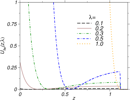
Figure 1: (Color online) Variation of the WCA wall potential as a function of $\lambda$ during the transformation of the bulk LJ liquid or crystal into an impenetrable flat wall interacting with the LJ system. From no wall at $\lambda=0$, we have a wall with a finite barrier at small values of $\lambda$. With increasing $\lambda$, the wall becomes more and more impenetrable. At $\lambda=1$, there is an impenetrable wall represented by the WCA potential.

To obtain $\gamma$ for a hard-sphere system in contact with a hard structureless wall via TI, Heni and Löwen heni99 have used a scheme, where a bulk hard sphere system is reversibly transformed into a system interacting with an impenetrable hard wall. In this work, we generalize the scheme of Heni and Löwen to continuous wall potentials. To this end, the wall potential is parametrized by a parameter $\lambda$ such that the wall changes smoothly from a penetrable to an impenetrable wall as $\lambda$ increases. The following parametrization of the wall potential is adopted:

$$\begin{split}u_{\text{fw}}(\lambda,z)=&\lambda^{2}4\epsilon_{\text{w}}\left[\left(\frac{\sigma_{\text{pp}}}{z+(1-\lambda)z_{\text{cw}}}\right)^{12}\right.\\ &\left.-\left(\frac{\sigma_{\text{pp}}}{z+(1-\lambda)z_{\text{cw}}}\right)^{6}+\frac{1}{4}\right]\times w(z).\end{split}$$ (17)

Figure 1, shows the parametrized wall potential at different values of $\lambda$. At $\lambda=0$ a bulk LJ system can freely cross the boundaries. For small values of $\lambda$ the barrier height at $z=0$ is of the same order as $k_{\text{B}}T$ and the LJ particles can penetrate the barrier. As $\lambda$ increases, the wall becomes more and more impenetrable and finally an impenetrable WCA wall is obtained at $\lambda=1$.

Since, the interfacial excess free energy of the LJ system in presence of walls is calculated with respect to a bulk LJ crystal, it is important that the bulk density is maintained as the parameter $\lambda$ is varied during the transformation. This is particularly important for a LJ liquid close to coexistence, since an increase in the bulk density in the presence of walls could lead to a precrystallization of the bulk liquid during the transformation, thus making it irreversible. A constant bulk density also ensures that our system is large enough such that there are no mutual influences between the walls on either side of the bulk LJ system. To maintain a constant bulk density one must keep the normal pressure $P_{\text{N}}$ constant and change the volume, as is achieved by carrying out simulation in the $NP_{\text{N}}AT$ ensemble.

The system Hamiltonian now depends on $\lambda$ and is given by

$$\begin{split}H({\bf r},{\bf p},\lambda)=\sum_{i=1}^{N_{\text{p}}}\frac{1}{2m_{i}}{{\bf p}_{i}^{2}}+\sum_{i=1}^{N_{\text{p}}}\sum_{j=i+1}^{N_{p}}u_{\text{pp}}({r_{ij}})+\\ \sum_{i=1}^{N_{\text{p}}}u_{\text{fw}}(\lambda,z=z_{i}-Z)\end{split}.$$ (18)

and thus the partition function can be written as

$$\begin{split}Q(\lambda)=\frac{1}{h^{3N}N!}\int\int\int\exp\left[-\frac{H({\bf r},{\bf p},\lambda)+P_{\text{z}}AL_{\text{z}}}{k_{\text{B}}T}\right]\\ \times AdL_{\text{z}}d\textbf{p}^{N}d\textbf{p}^{N}.\end{split}$$ (19)

The derivative of the Gibbs free energy with respect to $\lambda$ is

$$\frac{\partial G(\lambda)}{\partial\lambda}=-\frac{k_{\text{B}}T}{Q(\lambda)}\left[\frac{\partial Q(\lambda)}{\partial\lambda}\right]=\left\langle\frac{\partial H(\lambda)}{\partial\lambda}\right\rangle_{\lambda}\,$$ (20)

where the angular brackets denote the ensemble average at a particular value of $\lambda$ in the $NP_{\text{N}}AT$ ensemble.

The Gibbs free energy difference between the two initial and final state can then be obtained as

$$\Delta G =G(\lambda=1)-G(\lambda=0)=\int_{0}^{1}\left[\frac{\partial G(\lambda)}{\partial\lambda}\right]_{\lambda}d\lambda$$ (21)

$$=\int_{0}^{1}\left\langle\frac{\partial H(\lambda)}{\partial\lambda}\right\rangle_{\lambda}d\lambda\;.$$ (22)

To compute $\Delta G$ from molecular simulations, independent simulations runs are carried out at $N_{\lambda}$ discrete intervals between $\lambda=0$ and $\lambda=1$. Alternatively, one can also calculate the free energy difference in a single simulation by varying $\lambda$ step by step such that the final configuration at a value of $\lambda=\lambda_{i}$ is the initial configuration for the next value at $\lambda=\lambda_{i+1}$. In both methods, the system is equilibrated at each $\lambda=\lambda_{i}$, and then the time average of the quantity $\partial H(\lambda)/\partial\lambda$ is calculated. The numerical integration of Eq. (22) is carried out using the trapezoidal rule:

$$\Delta G=\sum_{i=1}^{N_{\lambda}-1}\frac{1}{2}\left[\left\langle\partial H/\partial\lambda\right\rangle_{i}+\left\langle\partial H/\partial\lambda\right\rangle_{i+1}\right](\lambda_{i+1}-\lambda_{i})\;.$$ (23)

The partial derivative of $H(\lambda)$ with respect to $\lambda$ is given by

$$\begin{split}\frac{\partial H(\lambda)}{\partial\lambda}=\frac{\partial u_{\text{fw}}(z,\lambda)}{\partial\lambda}=\frac{2}{\lambda}u_{\text{fw}}(\lambda,z)+\\ \frac{z_{\text{cw}}}{z+(1-\lambda)z_{\text{cw}}}u_{\text{fw}}(z,\lambda)\;.\end{split}$$ (24)

The above TI scheme leads to a wall which is not fully impenetrable and hence does not correspond to the desired state of interest at the end of the integration path. While the LJ particles cannot cross the wall at $\lambda=1$, two particles near the boundary but on opposite sides of the wall can still interact with each other. To overcome this problem another TI step is carried out to bring the system to a state where the LJ particles are in contact with a fully impenetrable wall excluding such spurious interactions. This is achieved by parametrizing $u_{\text{pp}}(r)$ by a factor $\mu$,

$$\begin{split}u_{\text{pp}}(\mu,r_{\text{ij}})={u_{\text{pp}}^{(1)}(r_{ij})}+(1-\mu){u_{\text{pp}}^{(2)}(r_{ij})}\end{split}$$ (25)

where, ${u_{\text{pp}}^{(1)}(r_{\text{ij}})}$ denotes interaction between LJ particles on same side of the wall, while ${U_{\text{pp}}^{(2)}(r_{ij})}$ corresponds to interaction between particles near the boundary but on opposite sides of the wall, i.e. the separation between particles is greater than $L_{z}/2$. At $\mu=0$, all such spurious interactions are taken into account. As $\mu$ increases such interactions are reduced by the factor $1-\mu$ and finally at $\mu=1$, these spurious interactions are completely neglected. The $\mu$ dependent Hamiltonian for this step can be written as,

$$\begin{split}H({\bf r},{\bf p},\mu)=\sum_{i=1}^{N_{\rm p}}\frac{1}{2m_{i}}{{\bf p}_{i}^{2}}+\\ \sum_{i=1}^{N_{\rm p}}\sum_{j=i+1}^{N_{p}}\left[u_{\text{pp}}^{(1)}(r_{ij})+(1-\mu)u_{\text{pp}}^{(2)}(r_{ij})\right]+\\ \sum_{i=1}^{N_{p}}u_{\text{fw}}(\lambda=1,z=z_{i}-Z)\;.\end{split}$$ (26)

The thermodynamic integrand in this step is

$$\partial H/\partial\mu=\partial u_{\rm pp}(r,\mu)/\partial\mu=-u_{pp}^{(2)}(r_{\text{ij}}).$$ (27)

and thus the free energy difference can be expressed as

$$\Delta G_{{\rm fw}\rightarrow{\rm fw}^{\ast}}=\int_{0}^{1}\langle\partial u_{\rm pp}(r,\mu)/\partial\mu\rangle_{\mu}d\mu.$$ (28)

Our simulations showed that the contribution of $\Delta G_{{\rm fw}\rightarrow{\rm fw}^{\ast}}$ is very minor, i.e. about 0.1% of $\Delta G$ from Eq. (23) and hence can be neglected.

Using Eqs. (12), (21), and (24), the interfacial free energy of a LJ system interacting with a flat wall can be written as

$$\gamma=\frac{G_{\text{fw}}-G_{\text{bulk}}}{A}=\frac{{\Delta G}_{\text{bulk}\rightarrow\text{fw}}}{A}$$ (29)

with

$${\Delta G}_{\text{bulk}\rightarrow\text{fw}}=\int_{0}^{1}\left\langle\frac{\partial u_{\text{fw}}(z,\lambda)}{\partial\lambda}\right\rangle_{\lambda}d\lambda.$$ (30)

In the second step of our TI scheme, the flat wall is reversibly transformed into a structured wall in contact with the LJ system. During this change, the flat walls are positioned at the same location as the structured wall layer closest to the LJ liquid or crystal and there is no interaction between the flat and structured walls. The transformation from flat walls to structured walls is accomplished by parametrizing the wall potential as:

$$U_{\rm wall}(r_{\text{ij}},\lambda)=(1-\lambda)^{2}\sum_{i}u_{\text{fw}}(z=z_{i}-Z)+\\ \lambda^{2}\sum_{i,j}u_{\text{pw}}({r_{\text{ij}}})\;.$$ (31)

Now, the $\lambda$-dependent Hamiltonian is

$$\begin{split}H({\bf r},{\bf p},\lambda)=\sum_{\text{i=1}}^{N_{\rm p}}\frac{1}{2m_{i}}{{\bf p}_{\text{i}}^{2}}+\sum_{\text{i=1}}^{N_{\rm p}}\sum_{\text{j=i+1}}^{N_{p}}u_{\text{pp}}(r_{\text{ij}})+\\ (1-\lambda^{2})\sum_{i=1}^{N_{\rm p}}u_{\text{fw}}(z=z_{i}-Z,\lambda)+\lambda^{2}\sum_{i=1}^{N_{\rm p}}\sum_{j=1}^{N_{\rm w}}u_{\text{pw}}(r_{\text{ij}})\end{split}$$ (32)

and the derivative of the Hamiltonian with respect to $\lambda$

$$\begin{split}\frac{\partial H}{\partial\lambda}=&\frac{\partial U_{\text{wall}}}{\partial\lambda}\\ =&2\left[(\lambda-1)\sum_{i}u_{\text{fw}}(z=z_{i}-Z)+\lambda\sum_{i=1}^{N_{\rm p}}\sum_{j=1}^{N_{\rm w}}u_{\text{pw}}(r_{\text{ij}})\right]\;.\end{split}$$ (33)

So, finally the interfacial free energy of the LJ system in contact with a structured wall (sw) is given by

$$\gamma_{\text{wc}}=\frac{G_{\text{sw}}-G_{\text{bulk}}}{A}=\frac{{\Delta G}_{\text{bulk}\rightarrow\text{fw}}}{A}+\frac{{\Delta G}_{\text{fw}\rightarrow\text{sw}}}{A}$$ (34)

with

$${\Delta G}_{\text{fw}\rightarrow\text{sw}}=\int_{0}^{1}\left\langle\frac{\partial U_{\text{wall}}(\lambda)}{\partial\lambda}\right\rangle_{\lambda}d\lambda\,.$$ (35)

III.4 Simulations

To integrate the equations of motion, the velocity form of the Verlet algorithm was used with a time step $\tau=0.005$ and, to maintain constant normal pressure, the Andersen barostat algorithm andersen80 was chosen. Periodic boundary conditions are employed in the $x$, $y$ and $z$ directions for the first step of the TI method where flat walls are considered. In the second step periodic boundary conditions are only used along the $x$ and $y$ directions. The PA simulations are carried out with periodic boundary conditions only along the $x$ and $y$ directions. The temperature was kept constant by drawing every 200 steps the velocity of the LJ particles from the Maxwell-Boltzmann distribution at the desired temperature.

During the $NP_{\rm N}AT$ simulations, the position of the flat or structured walls must be modified keeping the normal pressure $P_{\text{N}}$ constant. To ensure this, the flat walls are treated as particles of infinite mass and, at each time step, the wall position $z_{\text{fw}}$ is rescaled according to

$$Z(t+\Delta t)=Z(t)\times L_{\text{z}}(t+\Delta t)/L_{\text{z}}(t)\;.$$ (36)

Note that this method is similar to the “fluctuating wall” method proposed by Lupowski and van Swol lupkowski90 , maintaining a constant normal pressure in a MC simulation of LJ particles in presence of a structureless wall.

When a rigid structured wall interacts with the LJ system, the wall particles must not change their positions relative to each other, thereby changing the wall density. To circumvent this problem, the center of mass of the wall is changed at every time step according to Eq. (36). The position of the individual particles of the wall is then shifted such that they are at the same relative distance from the center of mass as at the beginning of the simulation.

To calculate $\gamma_{\rm wl}$ we consider systems of $4000$ particles. The structured walls contain between 200-1200 particles, depending on the orientation and the density of the wall. The total surface area of the simulation cell is about $A=200$, yielding a length along the $z$ direction of about $L_{\text{z}}=65$ at the various wall-liquid interaction strengths $\epsilon_{\rm pw}$ and structured wall densities $\rho_{\text{w}}$. $\gamma_{\rm wl}$ is computed at a normal pressure of $P_{\rm N}=3$ and temperature $T=2$. At the start of the simulation, the LJ particles were placed on ideal fcc lattice sites and the walls were inserted simultaneously. Then the system was allowed to melt and equilibrate at the desired pressure and temperature, before the calculations were performed.

To test for the presence of any finite size effects, we also performed simulations with up to 12000 particles and a total surface area of about $A=340$, but obtained identical results compared to the simulations carried out with the smaller system size. This shows that systems of $4000$ particles are large enough to avoid finite size effects in the calculation of interfacial free energies.

From previous works pertaining to hard sphere systems, it is well known that the (111) orientation of the crystal in contact with a planar hard wall (or a soft WCA wall) gives the lowest interfacial tension as compared to the (100) or (110) orientations courtemanche93 . At small undercoolings, the hard sphere fluid freezes into the (111) crystal near the wall dijkstra04 . Hence, we obtain interfacial free energies only for the (111) orientation of the fcc crystal phase in contact with the walls. Unlike the liquid, the crystal has a long-range order and, in order to prevent deformation of the crystal, the system size must be compatible with this order.

For the determination of $\gamma_{\rm wc}$, systems of 7056 particles and area around $A=450$ are considered. The number of structured wall particles ranges from $800$ to about $1200$, depending on the different wall densities. Only the (111) orientation of the crystal in contact with the (111) orientation of the structured wall along the interface normal was considered. The corresponding simulations to obtain the interfacial free energy of a crystal in contact with a flat wall are carried out with $3960$ particles with an area of around $A=200$. Simulations were also carried out with a system size of $6006$ particles and a total area of $A=300$ and there was only a marginal deviation ($<1\%$) in the value of $\gamma_{\rm wc}$ as compared to the smaller system.

For comparing results obtained by our approach with that of Tang-Harris tang95 and Grzelak-Errington grzelak08 , we performed simulations for their system with $4000$ liquid particles and $392$ structured wall particles at the temperature $T=0.9$. We considered a lateral system size of $10\times 10$ and the length of the box along the $z$ direction was kept at $60.5134$ to obtain a bulk liquid density of $0.661$, the value reported by Tang and Harris tang95 for their simulations. Simulations were performed at this fixed density in the $NVT$ ensemble. With this system size, the finite size effects were negligible. The liquid in contact with the flat wall [Eq. (4)] was used as the reference state to calculate $\gamma_{\rm wl}$ for the liquid in contact with the structured wall at the same bulk density and temperature.

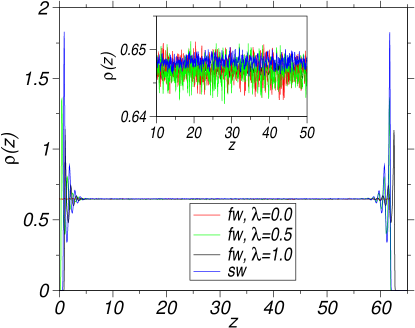
Figure 2: (Color online) Density profile of the system configuration for different values of $\lambda$ at the temperature $T=2.0$, the normal pressure $P_{\rm N}=3.0$, and the wall-liquid interaction strength $\epsilon_{\rm w}=1$. The corresponding density profile for a liquid in contact with the (100) orientation of a structured wall of density $\rho_{\rm w}=1.371$ at $\epsilon_{\rm pw}=1.0$ is also shown. The inset shows the density profiles in the bulk region on a magnified scale.

$\begin{array}[]{cc}\includegraphics[width=216.81pt]{fig3a.eps}&\includegraphics[width=216.81pt]{fig3b.eps}\end{array}$

Figure 3: (Color online) (a) $\langle\partial u_{\text{fw}}(z,\lambda)/\partial\lambda\rangle$ as a function of $\lambda$ computed from simulations at $P_{\rm N}=3$ and $T=2$ for the liquid and at $P_{\rm N}=3.0$ and $T=0.5$ in case of the crystal. To determine $\gamma_{\rm wl}$, $4000$ liquid particles were enclosed in a simulation box of area $A=200$ with the wall-liquid interaction strength $\epsilon_{\rm w}=1$. Corresponding simulations to calculate $\gamma_{\rm wc}$ were carried out with $3960$ particles and and area $A=235.22$. (b) $\langle\partial[U_{\rm wall}]/\partial\lambda\rangle$, corresponding to transformation of the flat wall into a structured wall. In case of the liquid, the structured wall consists of $392$ particles rigidly fixed to fcc lattice sites, with the (100) orientation of the wall facing the liquid. For the crystal, the structured wall consisted of $432$ wall particles with the (111) orientation of the wall in contact with the crystal. The density of the structured wall was $\rho_{\rm w}=1.371$ for the liquid ($\rho_{\rm rm}=0.647$ for the crystal) and the wall-particle interaction strength for the liquid -wall simulations was kept at $\epsilon_{\text{pw}}=1$, while for the crystal $\epsilon_{\rm pw}=0.5$. Other parameters are same as in (a).

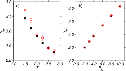
Figure 4: (Color online) (a) Interfacial free energy of liquid in contact with the flat wall, $\gamma_{\text{wl}}$, as a function of temperature. $NP_{N}AT$ simulations were carried out at a normal external pressure $P_{\text{N}}=3.0$, with $4000$ liquid particles and total surface area of $A=200$. The wall-liquid interaction strength is $\epsilon_{\rm w}=1$. Filled squares correspond to data obtained from TI, while estimates from PA are represented by open circles with error bars. Uncertainty in data computed by TI is less than the symbol size. (b) $\gamma_{\text{wl}}$ as a function of pressure at $T=2.5$. Other parameters and symbols representing the TI and PA data are same as in (a).

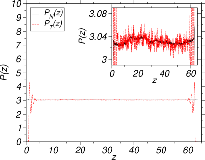
Figure 5: (Color online) Normal and tangential components of the pressure profiles of liquid in contact with a flat wall at $P_{\text{N}}=3$ and $T=2$, with $4000$ liquid particles. The wall liquid interaction strength, $\epsilon_{\rm w}=1$. Inset shows the pressure profiles on a magnified scale close to the magnitude of the external pressure $P_{\rm N}$.

A simulation at constant normal pressure leads to fluctuations of the length of the simulation cell in the $z$ direction, $L_{\text{z}}$. However, in order to compute the density and pressure profiles necessary for the PA method, it is more suitable to keep $L_{\text{z}}$ constant. Hence, to obtain $\gamma_{\rm wl}$ via the PA method, we first equilibrate the system in the $NP_{\rm N}AT$ ensemble for $5\times 10^{5}$ time steps. After equilibrium is reached, the simulations continue for $4.5\times 10^{6}$ time steps, from which the average length of the box in the $z$ direction is calculated. $L_{\rm z}$ is set to this average value and the particle coordinates are rescaled by the factor $\langle L_{\text{z}}\rangle/L_{\text{z}}(t_{\text{f}})$, $t_{\text{f}}$ denoting the time at the end of this equilibration run. An equilibration run is then carried out in the $NVT$ ensemble for $5\times 10^{5}$ time steps and the final production run consists of $4.5\times 10^{6}$ steps, when we accumulate data for the density, energy, temperature and pressure profiles every $5$ time steps, averaging the profiles over $9\times 10^{5}$ sample configurations. In our simulations, we observe a drift of $0.5-2.5\%$ in the normal pressure profile from the given external pressure $P_{\rm N}$. This drift can be reduced by averaging the length of the box for a longer simulation time or over a large number of realizations.

To calculate the interfacial free energy via TI, we used around $40$ intervals between $\lambda=0$ and $\lambda=1$ to numerically compute Eq. (23). Independent equilibration runs were carried out at each value of $\lambda$, in the $NP_{\text{N}}AT$ ensemble for about $5\times 10^{5}-1\times 10^{6}$ time steps. After the completion of the equilibration run, production runs were performed for $5\times 10^{5}$ steps in order to accumulate data. The same TI scheme and simulation procedure has been adopted to determine the interfacial free energy of the system investigated by Tang-Harris tang95 and Grzelak-Errington grzelak08 , but in the $NVT$ ensemble at a fixed liquid density.

For our TI method to be valid, there must be a bulk region unaffected by the wall. Figure 2 shows the density profile of liquid in contact with the parametrized flat wall represented by Eq. (17) at various values of $\lambda$, with the wall-liquid interaction strength $\epsilon_{\rm w}=1$. Also shown in Fig. 2 is the density profile of the liquid in contact with the (100) orientation of a structured wall of density $\rho_{\rm w}=1.371$ and with interaction strength $\epsilon_{\rm pw}=1$. The inset shows a magnified view of the density profiles in the bulk region. Clearly, all the density profiles overlap with each other indicating that the bulk region is unaffected by the walls.

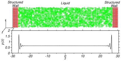
Figure 6: (Color online) a) A two-dimensional projection onto the $zy$ plane of a sample configuration of liquid in contact with the (100) orientation of the structured wall at $P_{\rm N}=3$ and $T=2$. $4000$ liquid particles are enclosed in a simulation box of area $A=200$. The density of the structured wall is $\rho_{\rm w}=1.371$. The wall-liquid interaction strength is set to $\epsilon_{\text{pw}}=1$. b) Density profile of the liquid, averaged over many configurations, showing pronounced layering at the structured wall-liquid interface.

$\begin{array}[]{cc}\includegraphics[width=216.81pt]{fig7a.eps}&\includegraphics[width=216.81pt]{fig7b.eps}\end{array}$

Figure 7: (Color online) a) Interfacial free energy of liquid in contact with the (100) orientation of the structured wall vs. $\epsilon_{\rm pw}$. All parameters are the same as in Fig. 6. Open squares with solid line represent data from the TI method and open circles with dashed line represent estimates yielded by the PA method. Uncertainties in data from TI are less than the symbol size. The wall-liquid interaction strength is $\epsilon_{\rm pw}=1$. b) Liquid density profiles at different wall-liquid interaction strengths. The inset shows the profiles corresponding to the (100), (110) and (111) orientations of the structured wall in contact with the liquid at $\epsilon_{\rm pw}=1$. For comparison the density profile for liquid in contact with the flat wall is also shown in both a) and b). All system parameters are same as in a).

Figure 3a shows the thermodynamic integrand $\langle\partial u_{{\text{fw}}}(z,\lambda)/\partial\lambda\rangle$ as a function of $\lambda$, during the transformation of a bulk liquid (crystal) to a confined liquid (crystal), interacting with flat walls. The integrand is smooth, thus allowing for an accurate determination of the interfacial free energy. Figure 3b shows the integrand as a function of $\lambda$ for the second step of the thermodynamic integration when the flat wall is transformed into a structured wall. The integrand is always negative, implying that the interfacial free energy of a LJ liquid (crystal) in contact with a rigid structured wall is smaller than for the case where the liquid (crystal) is in contact with a structureless flat wall.

IV Results

IV.1 $\gamma_{\rm wl}$

Using TI, we first determine the liquid-flat wall interfacial free energy $\gamma_{\rm wl}$ at several temperatures and pressures. In Fig. 4, we plot the data obtained from TI along with the estimate for $\gamma_{\rm wl}$ from the PA technique, as a function of temperature and pressure, respectively. The error bars in $\gamma_{\rm wl}$ obtained from TI are smaller than the symbol size and hence are not reported. It is evident from Fig. 4 that there is good agreement between the two methods within the statistical error. However, Fig. 4a shows that $\gamma_{\rm wl}$ obtained from TI is smoothly varying, while the PA data is less systematic. Relative differences between the two methods are between 0.3 and 1.8%.

This small disagreement between the two methods is due to the large fluctuations in the local pressure profiles as obtained from Eqs. (13) and (14) (see Fig. 5). The inset in Fig. 5 clearly shows the large fluctuations in the normal pressure profile near the wall and in both the normal and tangential pressure profiles in the bulk region. Since Eq. (10) represents the difference between two pressure profiles: Any lack of precision in the numerical measurements magnifies the relative error. The TI data is more accurate and less computationally expensive compared to what would be required to obtain more precise values from the PA method.

The liquid-flat wall system can now be used as the reference system to calculate the interfacial free energy of the liquid in contact with a rigid structured wall. Some properties of the structured wall such as the wall-liquid interaction strength, density of the structured wall and its orientation along the interface will affect the interfacial free energy and consequently the wetting behavior of the liquid. We will investigate $\gamma_{\rm wl}$ for the (100), (110) and, (111) orientations of the structured wall in contact with the liquid at different wall-liquid interaction strengths. Effects of density of the structured wall on the interfacial free energy will also be studied. Unless otherwise indicated, the external pressure is set to $P_{\rm N}=3$ and the temperature to $T=2$.

Figure 6 shows a sample configuration of the liquid in contact with the (100) orientation of a structured wall in the $zy$ plane and the corresponding density profile. We observe layering of the particles near the wall. Away from the walls a bulk region forms, where the density is constant.

In Fig. 7a, $\gamma_{\rm wl}$ is displayed as a function of $\epsilon_{\rm pw}$, as obtained from the PA and TI method. The error bars in the PA method were calculated from $2-3$ realizations. For TI, the error bars are smaller than the size of the symbols and hence they are not reported. We observe that $\gamma_{\rm wl}$ decreases with $\epsilon_{\rm pw}$, which is in agreement with previous studies carried out using the mechanical route nijmeijer90 ; tang95 and other thermodynamic methods leroy09 ; grzelak08 . High values of $\epsilon_{\rm pw}$ represent stronger attraction between the wall and liquid particles. This reduces the free energy needed to move the liquid from the bulk to the surface resulting in a lower interfacial free energy. Data from the two methods agree qualitatively but the percentage difference of the PA results with respect to the TI data increases at higher values of $\epsilon_{\rm pw}$.

Apart from the fluctuations in the local pressure profiles, the strong layering near the interface at large $\epsilon_{\rm pw}$ also reduces the numerical accuracy of the PA method. Figure 7b shows the liquid density profiles at various interaction strengths along with the corresponding profile in presence of a flat wall. The first peak in the density profile corresponding to the flat wall occurs at a greater distance from the wall as compared to the peaks arising out of the liquid-structured wall interaction. This can be attributed to the purely repulsive flat wall, which pushes the liquid further away from the walls compared to the structured walls.

	(100)		(110)		(111)
$\epsilon_{\rm pw}$	$\gamma_{\rm wl}^{\rm TI}$	$\gamma_{\rm wl}^{\rm PA}$	$\gamma_{\rm wl}^{\rm TI}$	$\gamma_{\rm wl}^{\rm PA}$	$\gamma_{\rm wl}^{\rm TI}$	$\gamma_{\rm wl}^{\rm PA}$
0.10	2.115	2.165$\pm$0.034	1.865	1.902$\pm$0.025	2.149	2.189$\pm$0.010
0.25	2.039	2.067$\pm$0.034	1.808	1.860$\pm$0.033	2.056	2.073$\pm$0.004
0.50	1.742	1.775$\pm$0.012	1.521	1.587$\pm$0.003	1.740	1.806$\pm$0.002
0.75	1.364	1.343$\pm$0.007	1.144	1.252$\pm$0.003	1.348	1.335$\pm$0.002
1.00	0.929	0.862$\pm$0.012	0.705	0.868$\pm$0.012	0.906	0.902$\pm$0.012

Table 1: Interfacial free energy $\gamma_{\rm wl}$ at different wall-liquid interaction strengths, for the (100), (110) and (111) orientations of the structured wall in contact with the liquid. Data computed from both TI and PA are shown. Simulations are carried out at $P_{\rm N}=3$ and $T=2$. The density of the structured wall $\rho_{\rm w}=1.371$.

The interfacial free energy of the crystal-melt interface is influenced by the orientation of the crystal in contact with the melt gibbs57 . Similarly, it might be expected that different orientations of the structured wall in contact with the liquid will affect the wall-liquid interfacial free energy. In the inset of Fig. 7b, we plot the density profiles near the wall for the (111), (110) and (100) orientations of the structured wall in contact with the liquid at $\epsilon_{\text{pw}}=1$. The density of the structured wall $\rho_{w}=1.371$ and, the lateral dimensions of the system corresponding to the (100), (110) and (111) orientations of the wall are $10\times 10$, $10\times 10.102$ and $9.623\times 10.102$, with $392$, $420$ and $330$ wall particles, respectively. Figure 7b shows the layering of the density profile to be most pronounced for the (111) orientation owing to the closely packed atoms exerting a greater repulsive force on the liquid. In contrast, the layering for the (110) orientation is much less pronounced and the first peak in the density profile also occurs closer to the wall as compared to the (111) or (100) orientations.

In Table I, we report $\gamma_{\text{wl}}$, obtained from the PA and TI methods, at various $\epsilon_{\text{pw}}$, for the (100), (110) and (111) orientations of the structured wall in contact with the liquid. In general, we find $\gamma_{\text{wl}}$ corresponding to the (111) and (100) orientations of the wall to be larger compared to the (110) orientation. This can be attributed to the stronger repulsive forces exerted on the liquid by the more close packed (111) and (100) planes, as compared to the more loosely packed (110) plane. Also, relatively better agreement is observed between the PA and TI methods for the (100) and (111) orientations of the wall as compared to the (110) orientation.

Simulations were also carried out for large system sizes at $\epsilon_{\rm pw}=1$, with up to $12000$ particles, and large surface area and wall separations. However, no systematic change was observed as compared to the smaller system size. Clearly, to obtain accurate values of the interfacial free energy, the pressure profiles need to be determined with far greater numerical accuracy. This has also been recently pointed out by D. Deb et al. deb11 for hard sphere systems. Computing the pressure profiles with high precision is computationally expensive and since accurate values can be obtained by the TI method with much less computational effort, use of the PA technique seems to be unjustified. In the remainder of the discussion on our model, we report results obtained with the TI method only.

$\begin{array}[]{cc}\includegraphics[width=216.81pt]{fig8a.eps}&\includegraphics[width=216.81pt]{fig8b.eps}\end{array}$

Figure 8: (Color online) a) Interfacial free energy of a liquid in contact with a structured wall vs. density of the wall at several wall-liquid interaction strengths $\epsilon_{\rm pw}$. Results were obtained from TI. Simulations were carried out at a constant normal pressure $P_{\text{N}}=3$ and temperature $T=2.0$. b) Density profiles of the liquid in contact with the structured wall at various densities $\rho_{w}$. The wall-liquid interaction strength is $\epsilon_{\text{pw}}=1$. Other parameters are same as in a).

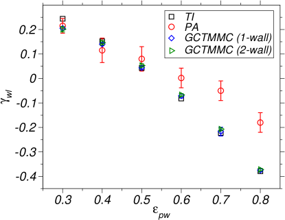
Figure 9: (Color online) $\gamma_{\text{wl}}$ vs. $\epsilon_{\text{pw}}$ for the model specified by Eq. (6). Squares correspond to our results computed via TI. Filled circles represent data from the studies of Tang-Harris tang95 , while diamonds and filled right triangles are the data obtained by Grzelak-Errington grzelak08 using the one-wall and two-wall approaches, respectively.

The density of the structured wall will also have an impact on the wetting behavior of the liquid in contact with it. We have carried out simulations at several densities $\rho_{\rm w}$ corresponding to different lattice constants of the ideal fcc lattice structure of the wall. In Fig. 8a, we report the TI results for $\gamma_{\rm wl}$ as a function of $\rho_{\rm w}$ at three different $\epsilon_{\rm pw}$’s. At $\epsilon_{\rm pw}=1$, the interfacial free energy decreases with the density of the wall. The larger number of wall particles at greater densities exert strong attractive forces on the liquid, reducing the interfacial free energy. At extremely large densities the interfacial free energy becomes negative indicating that the liquid completely wets the wall. No data for very low densities of the structured wall are shown in Fig. 8a since the liquid particles penetrate the wall at low densities and the interfacial region is no longer well defined.

At $\epsilon_{\rm pw}=0.5$, $\gamma_{\rm wl}$ shows a weak maximum and at large wall densities decreases with $\rho_{\rm w}$ more gradually as compared to the situation when $\epsilon_{\rm pw}=1$. At still lower wall-liquid interaction strength ($\epsilon_{\rm pw}=0.1$), $\gamma_{\rm wl}$ has a weak dependence on the density of the structured wall and remains almost constant in the range of $\rho_{w}$ shown in Fig. 8a.

In Fig. 8b, we show the density profiles of the liquid corresponding to several densities of the structured wall $\rho_{\rm w}$ at $\epsilon_{\rm pw}=1$. It is observed that the layering gets more pronounced and the first peak in the density profiles occurs further away from the walls as $\rho_{\rm w}$ increases. A similar behavior of the density profile was observed when increasing $\epsilon_{\rm pw}$ at fixed $\rho_{\rm w}$. The variation in $\gamma_{\rm wl}$ and the nature of the density profiles indicate that increasing $\rho_{\rm w}$ at $\epsilon_{\rm pw}=1$ has a similar effect on $\gamma_{\rm wl}$ as increasing $\epsilon_{\rm pw}$ at a fixed value of the wall density.

Finally, to compare results from our TI technique with those obtained by other methods, we consider the model defined by Eq. (6), which was first studied by Tang and Harris using a PA technique tang95 . Later Grzelak and Errington grzelak08 utilized GCTMMC simulations to obtain free energy profiles of the same system over a wide range of densities, with the fluid confined by a structured wall on one side and a hard wall at the other side or the fluid confined between two identical structured walls. Both of their approaches with one or two structured walls lead to the same results within the statistical errors. Using TI in the NVT ensemble, we computed the interfacial free energy of the same system, with the liquid confined by two identical structured walls. In Fig. 9, our results are reported along with data from the two previous works tang95 ; grzelak08 . Data obtained by Tang-Harris systematically deviate from our estimates of $\gamma_{\rm wl}$ as $\epsilon_{\rm pw}$ increases. Their data also has a large statistical error. However, our predictions are in good agreement with those of Grzelak and Errington.

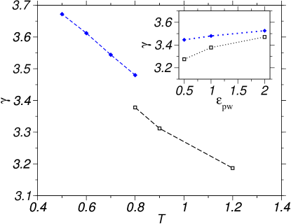
Figure 10: (Color online) Crystal-flat wall interfacial free energy $\gamma_{\rm wl}$ (diamonds) and liquid-flat wall interfacial excess free energy $\gamma_{\rm wc}$ (squares) as a function of temperature. $NP_{\rm N}AT$ simulations were carried out at $P_{\rm N}=3$ and the wall-liquid interaction strength $\epsilon_{\rm w}=1$. The (111) orientation of the crystal was considered in determining $\gamma_{\rm wc}$. Inset corresponds to $\gamma_{\rm wl}$ and $\gamma_{\rm wc}$ as a function of the interaction strength $\epsilon_{\rm w}$ at coexistence: $P_{\rm N}=3.0$ and $T=0.8$. Symbols are same as in the main graph.

IV.2 $\gamma_{\text{wc}}$

We will compute the crystal-wall interfacial energy by the TI method only, since the crystal can support stress and hence the interfacial tension and interfacial free energy are not the same, thus invalidating the applicability of the PA method tiller91 . In performing simulations of crystal in contact with walls on both sides, the number of particles $N$ must be chosen such that it is compatible with the long range order of the crystal. This is in contrast to a liquid, where choosing a large enough $N$ yields a sufficiently large system and the two walls on either side of the liquid do not influence each other. However, the crystal has a long-range order and merely choosing a large $N$ may not necessarily be commensurate with this order. Such an incommensurate $N$ is associated with long range elastic distortion, that propagates from one wall to the other leading to an inaccurate value for $\gamma_{\text{wc}}$. This had already been pointed out by D. Deb et al. deb10 who studied the interfacial free energy of a hard-sphere crystal confined between softly repulsive walls described by the WCA potential.

As specified earlier, we restrict our attention to the close-packed (111) orientation of the crystal in contact with a flat wall along the $z$ axis. To evaluate $\gamma_{\text{wc}}$, a bulk fcc crystal with the (111) orientation along $z$ axis is simulated in the $NPT$ ensemble. Periodic boundary conditions are employed in all directions to determine the average equilibrium lattice constant and hence the density of the crystal. A fcc crystal with this density was chosen as the initial configuration for the TI simulations to compute $\gamma_{\rm wc}$. The length of the simulation box was chosen such that an integer number of unit cells along the $x$, $y$ and $z$ directions adapted exactly into the simulation box. Then, independent simulations in the $NP_{\text{N}}AT$ ensemble were carried out at each value of the $\lambda$ parameter during the two-step TI scheme. In Fig. 10, we plot $\gamma_{\text{wc}}$ for crystal in contact with a flat wall, as a function of temperature up to the coexistence temperature at $P_{\rm N}=3.0$. For comparison, $\gamma_{\rm wl}$ is also plotted at the same pressure. Similar to $\gamma_{\rm wl}$, $\gamma_{\rm wc}$ decreases as a function of temperature.

To predict the wetting behavior of the crystal in contact with the wall at crystal-liquid coexistence, one needs $\gamma_{\text{cl}}$ in addition to $\gamma_{\text{wl}}$ and $\gamma_{\text{wc}}$. However, without knowledge of $\gamma_{\text{cl}}$, it is still possible to predict whether the crystal will completely wet the wall ($\theta_{\text{c}}=0^{\circ}$) or do so only partially ($0<\theta_{\text{c}}<180^{\circ}$). To this end, simulations were carried out at coexistence ($P_{N}=3.0,T=0.8$) for the bulk liquid and crystal in contact with a flat wall at various interaction strengths between the wall and the bulk liquid or crystal. The data is reported in the inset of Fig. 10. No wetting layer was observed near the walls during wall-liquid simulations, allowing for a determination of the wall-liquid interfacial free energy directly at coexistence. We find that $\gamma_{\text{wc}}>\gamma_{\text{wl}}$, showing that there is incomplete wetting of a flat wall by the (111) orientation of the LJ crystal and that the contact angle can be varied by changing $\epsilon_{\text{pw}}$.

While $\gamma_{\text{cl}}$ has not been determined in this work, Davidchack and Laird davidchack03 ; laird09 , obtained the crystal-liquid interfacial free energy at coexistence for a similar LJ model. The bulk liquid and crystal densities at the coexistence temperature $T=0.809$ for their model is same as for our system at $P_{\text{N}}=3.0$ and $T=0.8$. At $T=0.809$, they obtained $\gamma_{\text{cl}}=0.428\pm 0.004$. Since the LJ model used in this work is not very different from their potential, it is safe to assume that the crystal-liquid interfacial free energies will not be far apart. Using $\gamma_{\text{cl}}=0.428\pm 0.004$ and the values of $\gamma_{\text{wl}}$ and $\gamma_{\text{wc}}$ used in this work, we obtain contact angles of $97.4^{\circ}$, $103.8^{\circ}$ and $113.6^{\circ}$ respectively, signifying partial wetting of the flat wall. This is in contrast to the hard sphere case, where the (111) orientation of the crystal led to complete wetting of the wall deb10 . Such a situation of incomplete wetting will facilitate the study of heterogeneous nucleation of a crystal droplet at a wall-liquid boundary, and enable us to test the predictions of classical nucleation theory.

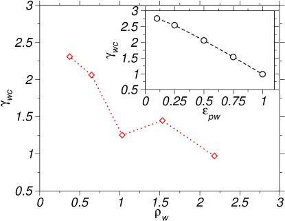
Figure 11: (Color online) Crystal-structured wall interfacial free energy, $\gamma_{\text{wc}}$, as a function of the structured wall density, for the (111) orientation of the crystal in contact with the (111) orientation of the structured wall. $NP_{N}AT$ simulations were carried out at a normal pressure and temperature $P_{\text{N}}=3$ and $T=0.5$ respectively, with the crystal-wall interaction strength $\epsilon_{\text{wc}}=0.5$. The inset shows $\gamma_{\text{wc}}$ as a function of $\epsilon_{pw}$ for a structured wall density $\rho_{w}=0.647$, other parameters remaining the same.

Having obtained the flat wall-crystal interfacial free energy, we can now compute the structured wall-crystal interfacial excess free energy $\gamma_{\text{wc}}$. We choose to investigate the (111) orientation of the crystal in contact with the (111) orientation of the structured wall. To obtain $\gamma_{\text{wc}}$, commensurate surfaces of the wall must be in contact with the crystal on both sides. We know that in the fcc structure, there is an $ABCABCABC...$ stacking of the lattice planes along the (111) orientation. The same order of the planes must be kept for the crystal plane in contact with the wall. For example, the the following stacking of the planes,

$$\begin{split}A_{\text{w}}B_{\text{w}}C_{\text{w}}A_{\text{w}}B_{\text{w}}C_{\text{w}}A_{\text{c}}B_{\text{c}}C_{\text{c}}A_{\text{c}}B_{\text{c}}C_{\text{c}}...\\ ......A_{\text{c}}B_{\text{c}}C_{\text{c}}A_{\text{w}}B_{\text{w}}C_{\text{w}}A_{\text{w}}B_{\text{w}}C_{\text{w}}.\end{split}$$ (37)

is commensurate. However, a stacking of the planes in an incommensurate manner such as

$$\begin{split}A_{\text{w}}B_{\text{w}}C_{\text{w}}A_{\text{w}}B_{\text{w}}C_{\text{w}}A_{\text{c}}B_{\text{c}}C_{\text{c}}A_{\text{c}}B_{\text{c}}C_{\text{c}}...\\ ......A_{\text{c}}B_{\text{c}}C_{\text{c}}C_{\text{w}}B_{\text{w}}A_{\text{w}}C_{\text{w}}B_{\text{w}}A_{\text{w}}\end{split}$$ (38)

will lead to long range deformation of the crystal.

In Fig. 11 and its inset, we plot $\gamma_{\text{wc}}$ as a function of the structured wall density and, in the inset, as a function of the wall-crystal interaction strength $\epsilon_{\rm pw}$. Similar to the liquid case we find that the interfacial free energy decreases with $\epsilon_{\rm pw}$ due to the stronger attraction between the crystal and the wall. Unlike the liquid case, Fig. 11 shows that while the main trend for $\gamma_{\rm wc}$ is to increase with decreasing density of the structured wall, there is a sharp dip when the density of the wall equals the density of the crystal. This is easy to understand, since less energy will be needed to create an interface, when the structured wall has the same structure as the crystal than when there is a mismatch between the wall and crystal structures leading to a relatively unfavorable interaction between them.

V Conclusion

We propose a thermodynamic integration (TI) scheme to compute interfacial free energies of liquids or crystals in contact with flat or structured walls from molecular dynamics simulation. In this work, this scheme has been applied to Lennard-Jones systems, but it can be easily generalized to other interaction models. The implementation of our method is simple, and, as demonstrated above, our method provides reliable and accurate estimates of $\gamma_{\rm wl}$ and $\gamma_{\rm wc}$ that enter in Young’s equation (1). In particular for structured walls (substrates), to the best of our knowledge, there are no simulation studies calculating the substrate-crystal interfacial free energy $\gamma_{\rm wc}$. Most of the previous simulation works on structured walls nijmeijer90 ; tang95 ; vanleeuwen90 ; bruin91 ; bakker89 ; crevecoeur95 have been limited to the calculation of the interfacial free energy $\gamma_{\rm wl}$ using the integration over the pressure anisotropy (PA). The PA method, however, does not give reliable results in general, and, in contrast to our TI scheme, it is not applicable to substrates that can support stress (such as structured walls where the wall particles are allowed to move and are thus not fixed to their ideal lattice positions, see discussion above). Therefore, the TI scheme proposed in this work can be considered as a novel approach to obtain accurate values for substrate-liquid or substrate-crystal interfacial free energies and thus it will be useful in studies of wetting and nucleation problems.

- (1) J. W. Gibbs, The Collected Works (Yale University Press, New Haven, CT, 1957), Vol. 1.
- (2) A. W. Adamson and A. P. Gast, Physical chemistry of surfaces (Wiley-Interscience, New York, 1997).
- (3) S. Dietrich, in Phase Transitions and Critical Phenomena, Vol. 12, edited by Domb and Lebowitz (Academic, New York, 1988).
- (4) J. S. Rowlinson and B. Widom, Molecular Theory of Capillarity (Clarendon, Oxford, 1982).
- (5) P. G. de Gennes, Rev. Mod. Phys. 57, 827 (1985); P. G. de Gennes, F. Brochart-Wyart, and D. Quéré, Capillarity and Wetting Phenomena. Drops, Bubbles, Pearls, Waves (Springer, New York, 2004).
- (6) G. Navascués, Rep. Prog. Phys. 42, 1131 (1979).
- (7) J. M. Howe, Interfaces in Materials (Wiley, New York, 1997); M. E. Glicksman and N. B. Singh, J. Cryst. Growth 98, 277 (1989); M. Muschol, D. Liu, and H. Z. Cummins, Phys. Rev. A 46, 1038 (1992).
- (8) M. P. Allen and D. J. Tildesley, Computer Simulations of Liquids (Clarendon, Oxford, 1987).
- (9) D. P. Landau and K. Binder, A Guide to Monte Carlo Simulations in Statistical Physics (Cambridge, USA, 2000).
- (10) H. Löwen, Phys. Rep. 237, 249 (1994); R. Evans, Liquids at Interfaces, Les Houches Session XLVIII, edited by J. Charvolin, J. F. Joanny, and J. Zinn-Justin (Elsevier, Amsterdam, 1990).
- (11) J. A. Barker and D. Henderson, Rev. Mod. Phys. 48, 587 (1976); B. Götzelmann, A. Haase, and S. Dietrich, Phys. Rev. E 53, 3456 (1996); H. Reiss, H. L. Frisch, E. Helfand, and J. L. Lebowitz, J. Chem. Phys. 32, 119 (1960); D. Henderson and M. Plischke, Proc. R. Soc. London, Ser. A 410, 409 (1987).
- (12) E. Velasco and P. Tarazona, J. Chem. Phys. 91, 7916 (1989); Yang-Xin Yu, J. Chem. Phys. 131, 024704 (2009).
- (13) J. R. Henderson and F. van Swol, Mol. Phys. 51, 991 (1984).
- (14) E. De Miguel and G. Jackson, Mol. Phys. 104, 3717 (2006).
- (15) M. J. P. Nijmeijer, C. Bruin, A. F. Bakker, and J. M. J. van Leeuwen, Phys. Rev. A 42, 6052 (1990).
- (16) J. Z. Tang and J. G. Harris, J. Chem. Phys. 103, 8201 (1995); J. G. Harris, J. Chem. Phys. 105, 4889 (1996).
- (17) M. J. P. Nijmeijer and J. M. J. van Leeuwen, J. Phys. A: Math. Gen. 23, 4211 (1990); J. H. Sikkenk, J. M. J. van Leeuwen, J. O. Indekeu, J. M. J. van Leeuwen, E. O. Vossnack, and A. F. Bakker, J. Stat. Phys. 52, 23 (1988).
- (18) M. J. P. Nijmeijer, C. Bruin, A. F. Bakker, and J. M. J. van Leeuwen, J. Phys.: Condens. Matter 4, 15 (1991).
- (19) F. Leroy, Daniel J. V. A. dos Santos, and F. Müller-Plathe, Macromol. Rapid Commun. 30, 864 (2009); F. Leroy and F. Müller-Plathe, J. Chem. Phys. 133, 044110 (2010).
- (20) J. H. Weijs, A. Marchand, B. Andreotti, D. Lohse, and J. Snoeijer, Phys. Fluids 23, 022001 (2011); L. Schimmele and S. Dietrich, Eur. Phys. J. E 30, 427 (2009); T. Getta and S. Dietrich, Phys. Rev. E 57, 655 (1998).
- (21) D. Frenkel and B. Smit, Understanding Molecular Simulation (Academic, San Diego, 2002); T. P. Straatsma, M. Zacharias, and J. A. MacCammon, Computer Simulations of Biomolecular Systems (Escom, Keiden, 1993).
- (22) J. G. Sampayao, A. Malijevský, E. A. Muller, E. De Miguel and G. Jackson, J. Chem. Phys. 132, 141101 (2010); P. R. ten Wolde and D. Frenkel, J. Chem. Phys. 109, 9901 (1998).
- (23) W. A. Tiller, The Science of Crystallization: Microscopic Interfacial Phenomena (Cambridge Univ. Press, New York, 1991).
- (24) F. Varnik, J. Baschnagel, and K. Binder, J. Chem. Phys. 113, 4444 (2000).
- (25) F. Varnik, Ph.D. Thesis (Mainz), 2000.
- (26) M. J. P. Nijmeijer, C. Bruin, A. F. Bakker, and J. M. J. Van Leeuwen, Physica A 160, 166 (1989).
- (27) M. J. P. Nijmeijer and C. Bruin, J. Chem. Phys. 103, 8201 (1995); C. Bruin, M. J. P. Nijmeijer, and R. M. Crevecoeur, J. Chem. Phys. 102, 7622 (1995).
- (28) B. B. Laird and R. L. Davidchack, J. Chem. Phys. 132, 204101 (2010).
- (29) M. Heni and H. Löwen, Phys. Rev. E 60, 7057 (1999).
- (30) A. Fortini and M. Dijkstra, J. Phys.: Condens. Matter 2006, 18, L371.
- (31) B. B. Laird and R. L. Davidchack, J. Phys. Chem. C 111, 15952 (2007).
- (32) D. Deb, A. Winkler, M. H. Yamani, M. Oettel, P. Virnau, and K. Binder, J. Chem. Phys. 134, 214706 (2011).
- (33) D. Deb, D. Wilms, A. Winkler, P. Virnau, and K. Binder, Int. J. Mod. Phys. C (2012).
- (34) F. G. Wang and D. P. Landau, Phys. Rev. Lett. 86, 2050 (2001).
- (35) G. Grochola, S. P. Russo, I. K. Snook, and I. Yarovsky, J. Chem. Phys. 117, 7676 (2002); G. Grochola, S. P. Russo, I. K. Snook, and I. Yarovsky, J. Chem. Phys. 117, 7685 (2002); G. Grochola, S. P. Russo, I. Yarovsky, and I. K. Snook, J. Chem. Phys. 120, 3425 (2004); G. Grochola, I. K. Snook, and S. P. Russo, J. Chem. Phys. 122, 174510 (2005); G. Grochola, I. K. Snook, and S. P. Russo, J. Chem. Phys. 122, 064711 (2005).
- (36) E. M. Grzelak and J. R. Errington, J. Chem. Phys. 128, 014710 (2008).
- (37) J. G. Kirkwood and F. P. Buff, J. Chem. Phys. 17, 338 (1949).
- (38) R. Shuttleworth, Proc. Phys. Soc. A 63, 444 (1950).
- (39) J. Irving and J. Kirkwood, J. Chem. Phys. 18, 817 (1950).
- (40) H. C. Andersen, J. Chem. Phys. 72, 2384 (1980).
- (41) M. Lupkowski and F. van Swol, J. Chem. Phys. 93, 737 (1990).
- (42) D. J. Courtemanche, T. A. Pasmore and F. van Swol, Mol. Phys. 80, 861 (1993).
- (43) M. Dijkstra, Phys. Rev. Lett. 93, 108303 (2004).
- (44) R. Davidchack and B. B. Laird, J. Phys. Chem. 118, 7657 (2003).
- (45) B. B. Laird, R. L. Davidchack, Y. Yang, and M. Asta, J. Chem. Phys. 131, 114110 (2009).