Evolutionary Processes in Finite Populations

Abstract

We consider the evolution of large but finite populations on arbitrary fitness landscapes. We describe the evolutionary process by a Markov, Moran process. We show that to $\mathcal{O}(1/N)$, the time-averaged fitness is lower for the finite population than it is for the infinite population. We also show that fluctuations in the number of individuals for a given genotype can be proportional to a power of the inverse of the mutation rate. Finally, we show that the probability for the system to take a given path through the fitness landscape can be non-monotonic in system size.

1 Introduction

Natural populations are characterized by finite sizes. For this reason, it is impossible for biology to sample the entire space of all possible genotypes. Even the number of possible sequences with high fitness is typically much larger than the population size in naturally occurring populations. Effects due to finite population size are particularly pronounced in asexual populations. For example, the reduction of fitness in a finite population without back mutation is termed Muller’s ratchet [1], and the decreased speed of evolution in a finite population without recombination is termed the the Hill-Robertson effect [2].

The relative influence of different evolutionary forces changes between small and large populations. While stochastic effects such as genetic drift act more strongly on small populations, natural selection acts more effectively on large populations. Many results in classical population genetics have focused on the limiting cases of small or infinite populations. In sufficiently small populations, beneficial mutations occur but rarely survive long enough to become established in the population. Those mutations that survive, however, can spread through a small population, reaching fixation, before another beneficial mutation arises. This regime is referred to as successional-mutations regime [3, 4] and is fairly well-understood. This theory has been useful, for example, to understand evolution of transcription factor binding sites [5]. As the population size increases, beneficial mutations arise more frequently. Fixation of individual mutations does not occur before the arrival of another beneficial mutation. In asexual populations this leads to competition between descendants of each of the mutations — an effect referred to as clonal interference [6]. As the population becomes even larger, ultimately stochastic effects become negligible, and the time-evolution of the evolving population can be described by a set of ordinary differential equations. This regime has been studied extensively in quasispecies theory, albeit often only for simple fitness functions.

Here we investigate the regime between clonal interference and quasispecies theory. We seek to predict the evolutionary dynamics followed by a large yet finite population and how this dynamics differs from that of an infinite population. The study of finite-population effects requires a stochastic description based on a master equation [7]. We make no assumption about the fitness landscape upon which the population evolves. We show that, averaged over time, the average fitness of a large finite population is lower than that of a population of infinite size. In other words, for large asexual populations evolving on a fixed fitness landscape, an increase in population size is accompanied by an increase in the average fitness. Furthermore, small mutation rates lead to high fluctuations and correlations. In particular, for small mutation rates, fluctuations and correlations in the number of individuals for a given genotype are inversely proportional to a power of the mutation rate. These large correlations enhance finite population effects and make the convergence to infinite-population behavior occur only for extremely large populations.

This article is organized as follows. We describe the stochastic process underlying our studies in section 2. We explain how this dynamic process can be written as a field theory. We derive analytic results for the infinite population evolution from this field theory. We describe finite population effects in section 3. We introduce the fitness landscape that we use to illustrate our results in section 4. In section 5 we investigate fluctuations in this random process. We verify our analytic results using stochastic simulations in section 2. We conclude in section 6.

2 Stochastic Process Mapped to a Field Theory

Throughout this article, we use the Moran process to model evolution of a population [8]. The individuals in the population are identified by their genotype, a sequence of length $l$. In this continuous-time process a constant population size, $N$, is maintained by simultaneous replication and death. The individual to be replicated is chosen randomly from the population with probability proportional to its microscopic fitness, while the individual to be killed is chosen randomly from the population with uniform probability. We further assume that replication and mutation are independent. Thus, there are two classes of events: mutation and replication. Mutation from genotype $i$ to genotype $j$ occurs at a rate of $\mu\Delta_{ij}N_{i}$, where $\mu$ is the mutation rate per locus, $N_{i}$ is the number of individuals with genotype $i$, and $\Delta_{ij}$ is equal to one if an individual can mutate from sequence $i$ to sequence $j$ with a single mutation and $\Delta_{ij}$ is equal to zero otherwise. This description allows for the incorporation of back-mutations which are often ignored in the literature. Note that the analytical results in this paper do not depend on this binary form of the matrix $\Delta$. Its elements can be arbitrary non-negative numbers as would be appropriate if back-mutation rates differed from forward mutation rates. Replication of genotype $i$ and simultaneous death of genotype $j$ occurs at a rate of $\frac{1}{N}r_{i}N_{i}N_{j}$, where $r_{i}$ is the replication rate of sequence $i$. The stochastic master equation for this process is

$$\frac{\partial}{\partial t}P(\boldsymbol{N};t) =\mu\sum_{i,j}\Delta_{ij}\left[\left(N_{i}+1\right)P(\boldsymbol{N}+\boldsymbol{e}_{i}-\boldsymbol{e}_{j};t)-N_{i}P(\boldsymbol{N};t)\right]$$

$$+\frac{1}{N}\sum_{i}r_{i}\sum_{j\neq i}\left[\left(N_{i}-1\right)\left(N_{j}+1\right)P(\boldsymbol{N}-\boldsymbol{e}_{i}+\boldsymbol{e}_{j};t)-N_{i}N_{j}P(\boldsymbol{N};t)\right].$$ (1)

Here $\boldsymbol{N}$ is a vector describing the state of the population by the number of individuals of each genoptype: $(N_{1},N_{2},\ldots)$, and $\boldsymbol{e}_{i}$ is a unit vector associated with genotype $i$. Note $\sum_{i}N_{i}=N$.

We obtain analytic expressions for the average occupation numbers and the fluctuations by mapping the stochastic process described in the previous section onto a field theory following [9]. To do this we introduce the state vector

$$\left|\psi(t)\right>=\sum_{\boldsymbol{N}}P(\boldsymbol{N};t)\left|\boldsymbol{N}\right>$$ (2)

whose time evolution is governed by

$$\frac{\partial}{\partial t}\left|\psi(t)\right> =\sum_{\boldsymbol{N}}\left[\mu\sum_{i,j}\Delta_{ij}\left[\left(N_{i}+1\right)P(\boldsymbol{N}+\boldsymbol{e}_{i}-\boldsymbol{e}_{j};t)-N_{i}P(\boldsymbol{N};t)\right]\right.$$

$$\qquad\left.+\frac{1}{N}\sum_{i}r_{i}\sum_{j\neq i}\left[\left(N_{i}-1\right)\left(N_{j}+1\right)P(\boldsymbol{N}-\boldsymbol{e}_{i}+\boldsymbol{e}_{j};t)-N_{i}N_{j}P(\boldsymbol{N};t)\right]\right]\left|\boldsymbol{N}\right>.$$ (3)

By defining annihilation and creation operators

$$\hat{a}_{i}\left|\boldsymbol{N}\right>=N_{i}\left|\boldsymbol{N}-\boldsymbol{e}_{i}\right>,\qquad\hat{a}_{i}^{\dagger}\left|\boldsymbol{N}\right>=\left|\boldsymbol{N}+\boldsymbol{e}_{i}\right>\qquad\hat{a}_{i}\hat{a}_{j}^{\dagger}-\hat{a}_{j}^{\dagger}\hat{a}_{i}=\delta_{ij},$$ (4)

we can write the governing equation for the state vector as

$$\frac{\partial}{\partial t}\left|\psi(t)\right>=-\hat{H}\left|\psi(t)\right>,$$ (5)

where

$$-\hat{H}=\mu\sum_{i,j}\Delta_{ij}\left(\hat{a}_{j}^{\dagger}-\hat{a}_{i}^{\dagger}\right)\hat{a}_{i}+\frac{1}{N}\sum_{i,j}r_{i}\hat{a}_{i}^{\dagger}\left(\hat{a}_{i}^{\dagger}-\hat{a}_{j}^{\dagger}\right)\hat{a}_{i}\hat{a}_{j}.$$ (6)

This differential equation has the formal solution

$$\left|\psi(t)\right>=e^{-\hat{H}t}\left|\psi(0)\right>,$$ (7)

where $\left|\psi(0)\right>=\left|\boldsymbol{N}^{0}\right>$ is the initial distribution of individuals in the population. At time $T$, the average of an observable represented by the (normal-ordered) operator $F(\{\hat{a}_{i}^{\dagger},\hat{a}_{i}\})$ can be obtained [10] by multiplying with the “sum bra” $\left<\cdot\right|=\left<0\right|(\prod_{i}e^{\hat{a}_{i}})$

$$\left<F\right>_{T}=\left<\cdot\right|F(\{\hat{a}_{i}^{\dagger},\hat{a}_{i}\})\left|\psi(T)\right>=\left<\cdot\vphantom{N^{0}}\right|F(\{\hat{a}_{i}^{\dagger},\hat{a}_{i}\})e^{-\hat{H}T}\left|\boldsymbol{N}^{0}\right>.$$ (8)

We introduce a Trotter factorization for the evolution operator $e^{-\hat{H}T}$, using a time interval $\epsilon\to 0$, in the basis of coherent states defined by $\hat{a}_{i}\left|\boldsymbol{z}\right>=z_{i}\left|\boldsymbol{z}\right>$ and obtain a path integral representation

$$\left<\cdot\vphantom{N^{0}}\right|F(\{\hat{a}_{i}^{\dagger},\hat{a}_{i}\})e^{-\hat{H}T}\left|\boldsymbol{N}^{0}\right> =\left<\cdot\vphantom{N^{0}}\right|F(\{\hat{a}_{i}^{\dagger},\hat{a}_{i}\})e^{-\epsilon\hat{H}}\cdot e^{-\epsilon\hat{H}}\cdot\,\cdots\,\cdot e^{-\epsilon\hat{H}}\left|\boldsymbol{N}^{0}\right>$$

$$=\int[Dz^{*}Dz]F(\{z(T/\epsilon)\})e^{-S(\boldsymbol{z},\boldsymbol{z}^{*})}.$$ (9)

Here, the action in the exponent is, after the change of variables $z_{i}^{*}\equiv 1+\bar{z}_{i}$,

$$S(\boldsymbol{z},\bar{\boldsymbol{z}}) =\sum_{i}\left[\sum_{k=0}^{T/\epsilon}\bar{z}_{i}(k)z_{i}(k)-\sum_{k=1}^{T/\epsilon}\bar{z}_{i}(k)z_{i}(k-1)-N_{i}(0)\ln\left(1+\bar{z}_{i}(0)\right)\right]$$

$$-\mu\epsilon\sum_{k=1}^{T/\epsilon}\sum_{i,j}\left(\bar{z}_{j}(k)-\bar{z}_{i}(k)\right)z_{i}(k-1)\Delta_{ij}$$

$$-\frac{\epsilon}{N}\sum_{k=1}^{T/\epsilon}\sum_{i,j}r_{i}\left(1+\bar{z}_{i}(k)\right)\left(\bar{z}_{i}(k)-\bar{z}_{j}(k)\right)z_{i}(k-1)z_{j}(k-1).$$ (10)

The population dynamics in the limit as the population size, $N$, becomes infinite emerges as a saddle point in the action [9]. Setting $\left.\delta S/\delta z_{i}(t)\right|_{c}=0$ leads to $\bar{z}_{i}^{c}(t)=0$. From setting $\left.\delta S/\delta\bar{z}_{i}(t)\right|_{c}=0$ we obtain $z_{i}^{c}(t)=Np_{i}(t)$ where $p_{i}(t)$ obeys the differential equation

$$\frac{dp_{i}}{dt}=\mu\sum_{j}\left(\Delta_{ji}p_{j}-\Delta_{ij}p_{i}\right)+r_{i}p_{i}-\left<r\right>p_{i}.$$ (11)

Here $\left<r\right>=\sum_{j}r_{j}p_{j}$ is the average fitness of the infinite population. This differential equation has the closed-form solution [11]

$$p_{i}(t)=\frac{\sum_{j}\left(e^{Yt}\right)_{ij}p_{j}(0)}{\sum_{a,j}\left(e^{Yt}\right)_{aj}p_{j}(0)},$$ (12)

where the matrix $Y$ is defined by $Y_{ij}=\mu\Delta_{ji}-\mu\delta_{ij}\sum_{k}\Delta_{ik}+\delta_{ij}r_{i}$.

3 Finite Population Shift to Probability Distribution

We proceed to quantify analytically how finite population effects alter the infinite population dynamics. To do so we expand the action about the saddle point and separate it into a Gaussian and a non-Gaussian part. Introducing $z_{i}(k)={z_{c}}_{i}(k)+\delta z_{i}(k)$ and $\bar{z}_{i}(k)=\delta\bar{z}_{i}(k)$ in Eq. 2 we can write $S=S_{0}+\Delta S$, where the reference action $S_{0}$ can be written as

$$S_{0}=\frac{1}{2}\boldsymbol{x}^{T}\cdot\Pi_{0}^{-1}\cdot\boldsymbol{x}$$ (13)

where

$$\boldsymbol{x}^{T}=\left(\{\delta\bar{\boldsymbol{z}}(0),\delta\boldsymbol{z}(0)\},\{\delta\bar{\boldsymbol{z}}(1),\delta\boldsymbol{z}(1)\},\cdots,\{\delta\bar{\boldsymbol{z}}(T/\epsilon),\delta\boldsymbol{z}(T/\epsilon)\}\right).$$ (14)

Here,

$$\Pi_{0}^{-1}=\left(\begin{array}[]{c|c|c|c|c}\left({\Pi_{0}^{-1}}\right)_{00}&-\left({\Pi_{0}^{-1}}\right)_{01}&0&0&\cdots\vphantom{\text{\huge X}}\\[4.0pt] \hline\cr-\left({\Pi_{0}^{-1}}\right)_{10}&\left({\Pi_{0}^{-1}}\right)_{11}&-\left({\Pi_{0}^{-1}}\right)_{12}&0&\cdots\vphantom{\text{\huge X}}\\[4.0pt] \hline\cr 0&-\left({\Pi_{0}^{-1}}\right)_{21}&\left({\Pi_{0}^{-1}}\right)_{22}&-\left({\Pi_{0}^{-1}}\right)_{23}&\ddots\vphantom{\text{\huge X}}\\[4.0pt] \hline\cr 0&0&-\left({\Pi_{0}^{-1}}\right)_{32}&\left({\Pi_{0}^{-1}}\right)_{33}&\ddots\vphantom{\text{\huge X}}\\[4.0pt] \hline\cr\vdots&\vdots&\ddots&\ddots&\ddots\vphantom{\text{\huge X}}\end{array}\right)$$ (20)

with

$$\left({\Pi_{0}^{-1}}\right)_{00}=\begin{pmatrix}\delta_{ij}N_{i}(0)&\delta_{ij}\\ \delta_{ij}&0\end{pmatrix}, \left({\Pi_{0}^{-1}}\right)_{kk}=\begin{pmatrix}-\epsilon(B)_{ij}&\delta_{ij}\\ \delta_{ij}&0\end{pmatrix},$$

$$\left({\Pi_{0}^{-1}}\right)_{k,k-1}=\begin{pmatrix}0&\delta_{ij}+\epsilon(A)_{ij}\\ 0&0\end{pmatrix}, \left({\Pi_{0}^{-1}}\right)_{k-1,k}=\begin{pmatrix}0&0\\ \delta_{ij}+\epsilon(A)^{T}_{ij}&0\end{pmatrix}.$$ (21)

The matrices $A$ and $B$ are

$$(A)_{ij} =\mu\Delta_{ji}-\mu\delta_{ij}\left(\sum_{m}\Delta_{im}\right)+\frac{1}{N}r_{i}{z_{c}}_{i}(k-1)+\delta_{ij}r_{i}$$

$$-\frac{1}{N}\delta_{ij}\left(\sum_{m}r_{m}{z_{c}}_{m}(k-1)\right)-\frac{1}{N}r_{j}{z_{c}}_{i}(k-1),$$ (22)

and

$$(B)_{ij}=2\delta_{ij}r_{i}{z_{c}}_{i}(k-1)-\frac{1}{N}\left(r_{i}+r_{j}\right){z_{c}}_{i}(k-1){z_{c}}_{j}(k-1).$$ (23)

The non-Gaussian part of the action is given by

$$\Delta S =-\sum_{i}N_{i}(0)\left[\ln\left(1+\delta\bar{z}_{i}(0)\right)-\delta\bar{z}_{i}(0)+\frac{1}{2}(\delta\bar{z}_{i}(0))^{2})\right]$$

$$-\frac{\epsilon}{N}\sum_{k=1}^{T/\epsilon}\sum_{i,j}\left[r_{i}\left(\delta\bar{z}_{i}(k)-\delta\bar{z}_{j}(k)\right)\delta z_{i}(k-1)\delta z_{j}(k-1)\right.$$ (24)

$$\qquad+r_{i}\delta\bar{z}_{i}(k)\left(\delta\bar{z}_{i}(k)-\delta\bar{z}_{j}(k)\right){z_{c}}_{i}(k-1)\delta z_{j}(k-1)$$

$$\qquad+r_{i}\delta\bar{z}_{i}(k)\left(\delta\bar{z}_{i}(k)-\delta\bar{z}_{j}(k)\right)\delta z_{i}(k-1){z_{c}}_{j}(k-1)$$

$$\qquad\left.+r_{i}\delta\bar{z}_{i}(k)\left(\delta\bar{z}_{i}(k)-\delta\bar{z}_{j}(k)\right)\delta z_{i}(k-1)\delta z_{j}(k-1)\right].$$

This formulation allows us to calculate averages using the Gaussian action and thermodynamic perturbation theory, which is equivalent to a cumulant expansion. The average occupation numbers are given by

$$\left<N_{i}\right>_{T} =\left<\cdot\vphantom{N^{0}}\right|\hat{a}_{i}^{\dagger}\hat{a}_{i}e^{-\hat{H}T}\left|\boldsymbol{N}^{0}\right>=\left<\cdot\vphantom{N^{0}}\right|\hat{a}_{i}e^{-\hat{H}T}\left|\boldsymbol{N}^{0}\right>=\int[Dz^{*}Dz]z_{i}(T/\epsilon)e^{-S(\boldsymbol{z},\bar{\boldsymbol{z}})}$$ (25)

$$=\int[Dz^{*}Dz]z_{i}(T/\epsilon)e^{-\Delta S}e^{-S_{0}}=\left<z_{i}(T/\epsilon)e^{-\Delta S}\right>_{0}$$ (26)

$$=\left<z_{i}(T/\epsilon)\right>_{0}-\left<z_{i}(T/\epsilon)\Delta S\right>_{0}+\frac{1}{2}\left<z_{i}(T/\epsilon)(\Delta S)^{2}\right>_{0}+\cdots$$ (27)

$$=Np_{i}(T)-\left<\delta z_{i}(T/\epsilon)\Delta S\right>_{0}+\frac{1}{2}\left<\delta z_{i}(T/\epsilon)(\Delta S)^{2}\right>_{0}+\cdots,$$ (28)

where the last step follows from $\left<(\Delta S)^{n}\right>_{0}=0$ $\forall n\in\mathbb{Z},n\geq 1$. This procedure leads to an asymptotic expansion for the occupation numbers in powers of $1/N$. To first order, we obtain

$$\frac{1}{N}\left<N_{a}\right>(T)\sim p_{a}(T)+\frac{1}{N^{2}}\int_{0}^{T}dt\,\sum_{i,j}{\Pi_{0}}^{z\bar{z}}_{ai}(T,t){\Pi_{0}}^{zz}_{ij}(t,t)\left(r_{i}-r_{j}\right).$$ (29)

This expansion about infinite size is accurate when the correction term on the right hand side of Eq. (29) is much smaller than $p_{a}(T)$. Equation (41) provides an estimate of the magnitude of the correction for a common landscape with $k$ intermediate steps. The second order term is given by Eq. A.1 in the appendix. We derive expressions for the matrices ${\Pi_{0}}^{z\bar{z}}_{ai}(T,t)$ and ${\Pi_{0}}^{zz}_{ij}(t,t)$ by inverting $\Pi_{0}^{-1}$ in Eq.  20. In continuous time for $T>t$, they obey

$$\frac{\partial{\Pi_{0}}^{z\bar{z}}(T,t)}{\partial T}=A(T){\Pi_{0}}^{z\bar{z}}(T,t),$$ (30)

with

$${\Pi_{0}}^{z\bar{z}}(t,t)=I$$ (31)

and

$$\frac{d{\Pi_{0}}^{zz}(t,t)}{dt}=B(t)+A(t){\Pi_{0}}^{zz}(t,t)+{\Pi_{0}}^{zz}(t,t)A^{T}(t),$$ (32)

with

$${\Pi_{0}}^{zz}_{ij}(0,0)=-\delta_{ij}N_{i}(0).$$ (33)

Using the expression for the first-order shift to the occupation numbers due to finite population effects, we calculate the finite population shift in the average fitness of the population. The average fitness correction is

$$\left<\delta r(T)\right> =\frac{1}{N^{2}}\int_{0}^{T}dt\,\sum_{i,j,a}r_{a}{\Pi_{0}}^{z\bar{z}}_{ai}(T,t){\Pi_{0}}^{zz}_{ij}(t,t)\left(r_{i}-r_{j}\right)$$ (34)

$$=-\frac{1}{N^{2}}\int_{0}^{T}dt\,\sum_{i,j,a}r_{a}{\Pi_{0}}^{z\bar{z}}_{ai}(T,t)\left({\Pi_{0}}^{zz}_{ij}(t,t)+N\delta_{ij}p_{i}(t)\right)r_{j},$$ (35)

This result shows that the correction to the mean fitness is $\mathcal{O}(1/N)$ the mean fitness in the limit of infinite population. This result can be rewritten in a more revealing form. Let $\bar{r}(t)$ be a random variable defined as

$$\bar{r}(t)\equiv\frac{1}{N}\sum_{i}r_{i}\left(N_{i}(t)-\left<N_{i}(t)\right>\right)$$ (36)

in the limit of large population size. The finite population correction to the average fitness can then be written as

$$\left<\delta r(T)\right> =-\int_{0}^{T}\left<\bar{r}(T)\,\bar{r}(t)\right>\,dt$$ (37)

and its time integral as

$$\int_{0}^{T}\left<\delta r(t)\right>\,dt=-\int_{0}^{T}dt\int_{0}^{t}dt^{\prime}\,\left<\bar{r}(t)\bar{r}(t^{\prime})\right>=-\frac{1}{2}\left<\left(\int_{0}^{T}\bar{r}(t)\,dt\right)^{2}\right>.$$ (38)

This expression for the average fitness correction, which resembles a fluctuation dissipation theorem, implies that the time-average of the finite-population shift is always negative. In other words, the average fitness of a large finite population is smaller than that of a population of infinite size. Note that this result is perturbative, valid for large population size $N$, and it does not require the average fitness to be a monotonic function of $N$ for small $N$. On complex fitness landscapes, it is possible for small asexual populations to achieve a higher average fitness than larger ones [12]. Nonetheless, for sufficiently large population sizes, the time-integrated average fitness increases monotonously with population size.

4 The Landscape

Figure 1: Left-hand side: the state-space for a fitness landscape with three forward-mutations and no back-mutations. Each node, $i$, is a particular genotype. The replication rate of each genotype is $r_{i}$. Right-hand side (discussed in Section 6): The state-space can be expanded to include mutational histories. Each two-mutation state is split into 2! = 2 states while the three-mutation state is split into 3! = 6 states. The node is now identified by a vector which conveys the mutational history of a particular path through the landscape.

The analytical expressions developed in this paper are applicable to arbitrary fitness landscapes and mutational pathways. However, we now describe in some detail the implications for fitness landscapes [13] defined by a certain number of fitness loci $l$ with two alleles each. Genotypes that differ from each other by exactly one point mutation in one of the loci are connected in the mutation matrix. Each position in sequence space is thus connected by a mutation event to $l$ other genotypes. Figure 1 shows the geometry of the landscape for the case of three loci. Typically in this landscape, the fitness of each state increases upon moving to the right in the figure.

5 Fluctuations around the Mean

The matrices ${\Pi_{0}}^{zz}(t,t)$ and ${\Pi_{0}}^{z\bar{z}}(T,t)$ can be understood intuitively. In the limit of large $N$, the off-diagonal elements of ${\Pi_{0}}^{zz}(t,t)$ describe the covariances between the occupation numbers at time $t$ while the diagonal elements are related to the variances of the occupation numbers at time $t$ by

$$\frac{1}{N^{2}}(\delta N_{a}(t))^{2}\sim\frac{1}{N}\left(p_{a}(t)+\frac{1}{N}{\Pi_{0}}^{zz}_{aa}(t,t)\right).$$ (39)

At different times, ${\Pi_{0}}^{zz}(T,t)$ gives the cross-covariances between the occupation numbers at times $T$ and $t$. The matrix ${\Pi_{0}}^{z\bar{z}}_{ai}(T,t)$ relates the correlations at different times to the same-time correlations via

$${\Pi_{0}}^{zz}(T,t)={\Pi_{0}}^{z\bar{z}}(T,t){\Pi_{0}}^{zz}(t,t).$$ (40)

We observe numerically that for small mutation rates, the fluctuations are proportional to a negative power of the mutation rate. Specifically,

$$\frac{1}{N^{2}}(\delta N_{a}(t))^{2}\sim\frac{1}{N}\left(\frac{r}{\mu}\right)^{k},$$ (41)

where $k$ is the number of mutational steps as shown in Fig. 2. This dependence can also be shown analytically for sufficiently simple landscapes. See section B in the appendix for one example. Thus the expansion, which naively appears to be in $1/N$ is actually in $1/(N\mu^{k})$. Thus, the expansion breaks down when $\mu<1/N^{1/k}$. The expansion is valid for large $N$ and $\mu\gg 1/N^{1/k}$.

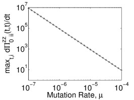
(a)

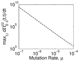
(b)

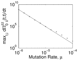
(c)

Figure 2: The maximal change of the variance with time (+), i.e. $\max_{t,i}d{\Pi_{0}}^{zz}_{ii}(t,t)/dt$ where ${\Pi_{0}}^{zz}$ is obtained from Eqs. 32 and 33, depends on the mutation rate as an inverse power law. Shown are calculations for a non-epistatic version of the landscape as described in section 4 with a) two possible mutations — $r_{0}=0,\Delta r_{1}\approx 0.049,\Delta r_{2}\approx 0.010$, b) three possible mutations — $r_{0}=0,\Delta r_{1}\approx 0.049,\Delta r_{2}\approx 0.010,\Delta r_{3}\approx 0.002$ — and c) four possible mutations — $r_{0}=0,\Delta r_{1}\approx 0.049,\Delta r_{2}\approx 0.020,\Delta r_{3}\approx 0.006,\Delta r_{4}\approx 0.002$. In this case, the fitness of each state is simply the sum of contributions from each mutation. The solid lines indicate power law fits using the values for $\mu\leq 10^{-5}$. Their exponents are a) -1.999, b) -2.989, and c) -3.939. The exponent is observed to be equal to the number of mutational steps in the landscape.

We verify our analytical results by performing stochastic simulations using the Lebowitz/Gillespie algorithm [14, 15]. Rewriting Eq. 29 for the first order shifts to the occupation numbers,

$$\left<N_{a}\right>(T)-Np_{a}(T)\sim\frac{1}{N}\int_{0}^{T}dt\,\sum_{i,j}{\Pi_{0}}^{z\bar{z}}_{ai}(T,t){\Pi_{0}}^{zz}_{ij}(t,t)\left(r_{i}-r_{j}\right),$$ (42)

we observe that the finite population correction converges to a constant value for large $N$. The average replication rate in the population is linear in the occupation numbers. It is equal to $\frac{1}{N}\sum_{i}r_{i}N_{i}(t)$. Therefore, the average replication rate also converges to the quasispecies result in the limit of a large population. That is, the average replication rate is equal to that of the infinite population plus a correction that is of order $1/N$ smaller. Figure 3 shows this convergence for one set of parameters. As a further check on our analytic results, we fit a cubic polynomial in $1/N$ to the simulation data displayed in Fig. 3. For the particular fitness parameters chosen here, the coefficients from this fit are $320.4\pm 2.5$ for the constant term and $(-5.3\pm 0.8)\times 10^{5}$ for the linear term, while our theory predicts $319.0$ and $-5.2\times 10^{5}$, respectively. Here, the coefficient of the linear term is obtained from Eq. A.1 in Appendix A.

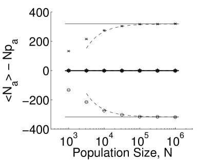
(a)

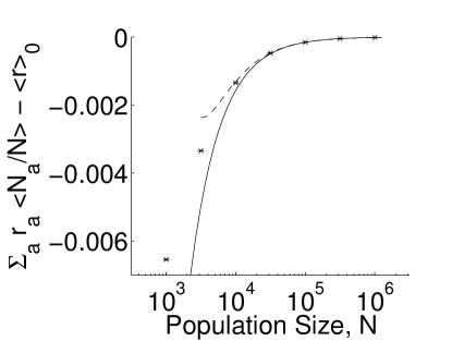
(b)

Figure 3: (a) Finite-population correction to the average occupation numbers (left-hand side of Eq. 42) as a function of population size, $N$, on a three-mutation landscape as shown in Fig. 1 including back-mutations. Shown are data for a mutation rate of $\mu=10^{-5}$ and replication rates of $r_{0}=0,r_{1}\approx 0.049,r_{2}\approx 0.010,r_{3}\approx 0.002,r_{4}\approx 0.059,r_{5}\approx 0.051,r_{6}\approx 0.012$, and $r_{7}\approx 0.061$. The time is chosen as $T=157.5$ which approximately maximizes $\left<N_{0}\right>(T)-Np_{0}(T)$. As $N$ increases, the corrections obtained from stochastic simulations — $N_{0}(\times)$, $N_{1}(\bigcirc)$, $N_{2}(+)$, $N_{3}(\ast)$, $N_{4}(\Box)$, $N_{5}(\Diamond)$, $N_{6}(\bigtriangledown)$, $N_{7}(\bigtriangleup)$ — converge to the values predicted by the theory (solid lines). The dashed curves show the second order expansion, given by Eqs. 42 and A.1. The error bars are one standard error. (b) Finite-size correction to the mean population fitness. The average replication rate in the population is linear in the occupation numbers, being equal to $\frac{1}{N}\sum_{i}r_{i}N_{i}(t)$, and so it too converges to the quasispecies result in the limit of a large population.

Similarly, we observe that the variances obtained from stochastic simulations agree with the analytic expression given in Eq. 39 as shown in Fig. 4.

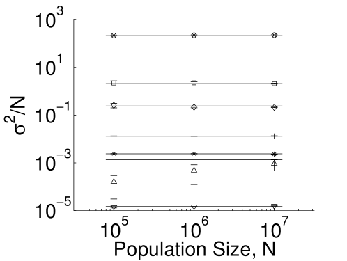
Figure 4: Variances divided by population size, $N$ as a function of $N$. The values obtained from stochastic simulations — $N_{0}(\times)$, $N_{1}(\bigcirc)$, $N_{2}(+)$, $N_{3}(\ast)$, $N_{4}(\Box)$, $N_{5}(\Diamond)$, $N_{6}(\bigtriangledown)$, $N_{7}(\bigtriangleup)$ — agree with the values predicted by Eq. 39 (solid lines). The time and other parameters are the same as in Fig. 3. The error bars are one standard error.

6 Discussion and Conclusion

Although the theory described in this paper was developed to study the time-evolution of the occupation numbers in sequence space, we can immediately apply these results to investigate which mutational paths individuals take. This allows us to predict the large $N$ behavior of the probability that a population will follow a certain mutational trajectory. To do this we simply expand the state space describing the identity of each individual to include not only the possible sequences but also the mutational histories. Figure 1 illustrates this expansion for the case of three mutations. Figure 5 compares the probability of following a given path as obtained from stochastic simulations to the expressions given in Eqs. 29 and A.1. We again observe that the simulation results converge to the values predicted by the theory as the population size increases. Interestingly, we observe numerically that the probability for a population to take a certain mutational path varies with the population size in a non-monotonic fashion. In particular, there is an intermediate population size at which the population is most likely to take the dominant path through the landscape.

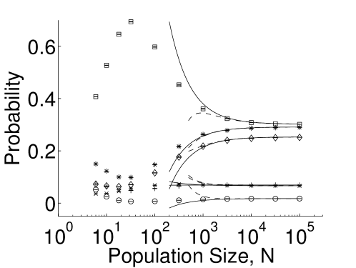
Figure 5: Probability that a population will follow a certain mutational trajectory as a function of population size. Shown are data for the landscape in Fig. 1 excluding back-mutations with a mutation rate of $\mu=10^{-3}$ and epistatic replication rates of $r_{0}=0,r_{1}\approx 0.049,r_{2}\approx 0.010,r_{3}\approx 0.002,r_{4}\approx 0.012,r_{5}\approx 0.051,r_{6}\approx 0.059$, and $r_{7}\approx 0.061$. Equation 42 (solid lines) predicts the asymptotic behavior of the simulation values — $N_{123}(\times)$, $N_{213}(\bigcirc)$, $N_{132}(\Box)$, $N_{312}(+)$, $N_{231}(\ast)$, $N_{321}(\Diamond)$ — for large population sizes. The second order expansion (dashed lines) improves the prediction for sufficiently large populations. The error bars are one standard error.

Fluctuations due to finite population can be quite large. As shown in Appendix B, these fluctuations are proportional to an inverse power of the mutation rate. That is, the expansion in $1/N$ has a coefficient that depends on a power of the inverse of the mutation rate. For this reason, convergence to the infinite population limit can be exceedingly slow. The coefficient in the expansion in $1/N$ also has a time dependence. As shown in Appendix C, this coefficient can be proportional to $t$, and so diverge at long times. This divergence occurs when there are multiple final states, with equal replication rates. For example, the fluctuations diverge at long times in the expanded state space due to what may be termed fixation of path probabilities.

In this paper we presented a path-integral formulation of evolution under a Moran-type process on arbitrary fitness landscapes. We derived analytic results that describe the dynamics exactly in the limit of an infinite population size and obtained an asymptotic expansion in the inverse of the population size for finite populations. We showed that the finite population correction to the time-averaged fitness is always negative, which implies that for sufficiently large population sizes the time-averaged fitness increases with population size. We also found that for small mutation rates, the infinite-population variances of the occupation numbers behave as $\mu^{-k}$ where $k$ is the number of mutational steps from the ancestral sequence. Finally, we showed how the formalism described in this paper can also be used to investigate which mutational path a population takes through the fitness landscape by expanding the sequence space to include mutational histories.

Appendix A Second Order Correction

Equation 29 gives the terms up $\mathcal{O}(N^{0})$ of an asymptotic expansion for the average occupation numbers in powers of $1/N$. We here determine the second order, $\mathcal{O}(N^{-1})$ correction terms. Figure A.1 shows all possible vertices appearing in the diagrams.

(a)

(b)

(c)

(d)

(e)

Figure A.1: Vertices for the diagrammatic expansion. A white circle represents an open time, while black circles stand for times that are integrated over.

Unlike the first correction term, which is derived from only the single non-vanishing diagram shown in Fig. A.2,

Figure A.2: Diagram for the $\mathcal{O}(N^{0})$ correction to the average occupation numbers.

the second order correction term comes from the nine different diagrams shown in Fig. A.3.

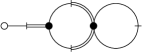
(a) Multiplicity: 2

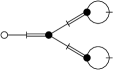
(b) Multiplicity: 1

(c) Multiplicity: 2

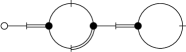
(d) Multiplicity: 4

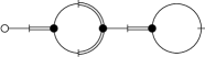
(e) Multiplicity: 2

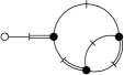
(f) Multiplicity: 8

(g) Multiplicity: 4

(h) Multiplicity: 8

(i) Multiplicity: 12

Figure A.3: Diagrams for the $\mathcal{O}(N^{-1})$ correction to the average occupation numbers with their multiplicities.

We obtain

$$\frac{1}{N}\left<N_{a}\right>(T)\sim p_{a}(T)+\frac{1}{N^{2}}\int_{0}^{T}dt\,\sum_{i,j}{\Pi_{0}}^{z\bar{z}}_{ai}(T,t){\Pi_{0}}^{zz}_{ij}(t,t)\left(r_{i}-r_{j}\right)+\frac{1}{N}\left<N_{a}\right>^{(2)}(T),$$ (A.1)

where

$$\left<N_{a}\right>^{(2)}(T)$$

$$=\frac{1}{2N^{2}}\int_{0}^{T}dt\,\sum_{i,j}\left({\Pi_{0}}^{z\bar{z}}_{ai}(T,t)-{\Pi_{0}}^{z\bar{z}}_{aj}(T,t)\right)\left(r_{i}-r_{j}\right)$$

$$\hskip 122.85876pt\int_{0}^{t}dt^{\prime}\,\sum_{i^{\prime},j^{\prime}}r_{i^{\prime}}\left({\Pi_{0}}^{z\bar{z}}_{ii^{\prime}}(t,t^{\prime})-{\Pi_{0}}^{z\bar{z}}_{ij^{\prime}}(t,t^{\prime})\right){\Pi_{0}}^{z\bar{z}}_{ji^{\prime}}(t,t^{\prime}){\Pi_{0}}^{zz}_{i^{\prime}j^{\prime}}(t^{\prime},t^{\prime})$$

$$+\frac{1}{4N^{3}}\int_{0}^{T}dt\,\sum_{i,j}\left({\Pi_{0}}^{z\bar{z}}_{ai}(T,t)-{\Pi_{0}}^{z\bar{z}}_{aj}(T,t)\right)\left(r_{i}-r_{j}\right)$$

$$\hskip 86.72377pt\int_{0}^{t}dt^{\prime}\,\sum_{i^{\prime},j^{\prime}}\left({\Pi_{0}}^{z\bar{z}}_{ii^{\prime}}(t,t^{\prime})-{\Pi_{0}}^{z\bar{z}}_{ij^{\prime}}(t,t^{\prime})\right)\left(r_{i^{\prime}}-r_{j^{\prime}}\right)\int_{0}^{t^{\prime}}dt^{\prime\prime}\,\sum_{i^{\prime\prime},j^{\prime\prime}}\left(r_{i^{\prime\prime}}-r_{j^{\prime\prime}}\right)$$

$$\hskip 122.85876pt\left[\left({\Pi_{0}}^{z\bar{z}}_{ji^{\prime\prime}}(t,t^{\prime\prime})-{\Pi_{0}}^{z\bar{z}}_{jj^{\prime\prime}}(t,t^{\prime\prime})\right)\left({\Pi_{0}}^{zz}_{i^{\prime}j^{\prime}}(t^{\prime},t^{\prime}){\Pi_{0}}^{zz}_{i^{\prime\prime}j^{\prime\prime}}(t^{\prime\prime},t^{\prime\prime})\right.\right.$$

$$\left.\hskip 260.17244pt+2{\Pi_{0}}^{zz}_{i^{\prime}j^{\prime\prime}}(t^{\prime},t^{\prime\prime}){\Pi_{0}}^{zz}_{j^{\prime}i^{\prime\prime}}(t^{\prime},t^{\prime\prime})\right)$$

$$\hskip 122.85876pt+2\left({\Pi_{0}}^{z\bar{z}}_{i^{\prime}i^{\prime\prime}}(t^{\prime},t^{\prime\prime})-{\Pi_{0}}^{z\bar{z}}_{i^{\prime}j^{\prime\prime}}(t^{\prime},t^{\prime\prime})\right)\left({\Pi_{0}}^{zz}_{jj^{\prime}}(t,t^{\prime}){\Pi_{0}}^{zz}_{i^{\prime\prime}j^{\prime\prime}}(t^{\prime\prime},t^{\prime\prime})\right.$$

$$\left.\left.\hskip 260.17244pt+2{\Pi_{0}}^{zz}_{ji^{\prime\prime}}(t,t^{\prime\prime}){\Pi_{0}}^{zz}_{j^{\prime}j^{\prime\prime}}(t^{\prime},t^{\prime\prime})\right)\right]$$

$$+\frac{1}{N^{3}}\int_{0}^{T}dt\,\sum_{i,j}\left({\Pi_{0}}^{z\bar{z}}_{ai}(T,t)-{\Pi_{0}}^{z\bar{z}}_{aj}(T,t)\right)\left(r_{i}-r_{j}\right)$$ (A.2)

$$\hskip 49.14307pt\int_{0}^{t}dt^{\prime}\,\sum_{i^{\prime},j^{\prime}}\left({\Pi_{0}}^{z\bar{z}}_{ii^{\prime}}(t,t^{\prime})-{\Pi_{0}}^{z\bar{z}}_{ij^{\prime}}(t,t^{\prime})\right)\left(r_{i^{\prime}}-r_{j^{\prime}}\right)\int_{0}^{t^{\prime}}dt^{\prime\prime}\,\sum_{i^{\prime\prime},j^{\prime\prime}}r_{i^{\prime\prime}}$$

$$\hskip 72.26999pt\left[{\Pi_{0}}^{z\bar{z}}_{ji^{\prime\prime}}(t,t^{\prime\prime})\left({\Pi_{0}}^{z\bar{z}}_{j^{\prime}i^{\prime\prime}}(t^{\prime},t^{\prime\prime})-{\Pi_{0}}^{z\bar{z}}_{j^{\prime}j^{\prime\prime}}(t^{\prime},t^{\prime\prime})\right)\left({\Pi_{0}}^{zz}_{i^{\prime}i^{\prime\prime}}(t^{\prime},t^{\prime\prime}){z_{c}}_{j^{\prime\prime}}(t^{\prime\prime})+{\Pi_{0}}^{zz}_{i^{\prime}j^{\prime\prime}}(t^{\prime},t^{\prime\prime}){z_{c}}_{i^{\prime\prime}}(t^{\prime\prime})\right)\right.$$

$$\hskip 72.26999pt+{\Pi_{0}}^{z\bar{z}}_{j^{\prime}i^{\prime\prime}}(t^{\prime},t^{\prime\prime})\left({\Pi_{0}}^{z\bar{z}}_{ji^{\prime\prime}}(t,t^{\prime\prime})-{\Pi_{0}}^{z\bar{z}}_{jj^{\prime\prime}}(t,t^{\prime\prime})\right)\left({\Pi_{0}}^{zz}_{i^{\prime}i^{\prime\prime}}(t^{\prime},t^{\prime\prime}){z_{c}}_{j^{\prime\prime}}(t^{\prime\prime})+{\Pi_{0}}^{zz}_{i^{\prime}j^{\prime\prime}}(t^{\prime},t^{\prime\prime}){z_{c}}_{i^{\prime\prime}}(t^{\prime\prime})\right)$$

$$\hskip 72.26999pt+\left.{\Pi_{0}}^{z\bar{z}}_{j^{\prime}i^{\prime\prime}}(t^{\prime},t^{\prime\prime})\left({\Pi_{0}}^{z\bar{z}}_{i^{\prime}i^{\prime\prime}}(t^{\prime},t^{\prime\prime})-{\Pi_{0}}^{z\bar{z}}_{i^{\prime}j^{\prime\prime}}(t^{\prime},t^{\prime\prime})\right)\left({\Pi_{0}}^{zz}_{ji^{\prime\prime}}(t,t^{\prime\prime}){z_{c}}_{j^{\prime\prime}}(t^{\prime\prime})+{\Pi_{0}}^{zz}_{jj^{\prime\prime}}(t,t^{\prime\prime}){z_{c}}_{i^{\prime\prime}}(t^{\prime\prime})\right)\right]$$

$$+\frac{1}{N^{3}}\int_{0}^{T}dt\,\sum_{i,j}\left({\Pi_{0}}^{z\bar{z}}_{ai}(T,t)-{\Pi_{0}}^{z\bar{z}}_{aj}(T,t)\right)\left(r_{i}-r_{j}\right)$$

$$\hskip 122.85876pt\int_{0}^{t}dt^{\prime}\,\sum_{i^{\prime},j^{\prime}}r_{i^{\prime}}\int_{0}^{t^{\prime}}dt^{\prime\prime}\,\sum_{i^{\prime\prime},j^{\prime\prime}}{\Pi_{0}}^{zz}_{i^{\prime\prime}j^{\prime\prime}}(t^{\prime\prime},t^{\prime\prime})\left(r_{i^{\prime\prime}}-r_{j^{\prime\prime}}\right)$$

$$\hskip 122.85876pt{\Pi_{0}}^{z\bar{z}}_{ii^{\prime}}(t,t^{\prime})\left({\Pi_{0}}^{z\bar{z}}_{ji^{\prime}}(t,t^{\prime})-{\Pi_{0}}^{z\bar{z}}_{jj^{\prime}}(t,t^{\prime})\right)\left({\Pi_{0}}^{z\bar{z}}_{i^{\prime}i^{\prime\prime}}(t^{\prime},t^{\prime\prime}){z_{c}}_{j^{\prime}}(t^{\prime})+{\Pi_{0}}^{z\bar{z}}_{j^{\prime}i^{\prime\prime}}(t^{\prime},t^{\prime\prime}){z_{c}}_{i^{\prime}}(t^{\prime})\right)$$

$$+\frac{2}{N^{2}}\int_{0}^{T}dt\,\sum_{i,j}\left({\Pi_{0}}^{z\bar{z}}_{ai}(T,t)-{\Pi_{0}}^{z\bar{z}}_{aj}(T,t)\right)\left(r_{i}-r_{j}\right)\int_{0}^{t}dt^{\prime}\,\sum_{i^{\prime},j^{\prime}}{\Pi_{0}}^{z\bar{z}}_{ii^{\prime}}(t,t^{\prime})\left(r_{i^{\prime}}-r_{j^{\prime}}\right)$$

$$\hskip 122.85876pt\sum_{i^{\prime\prime}}{\Pi_{0}}^{z\bar{z}}_{ji^{\prime\prime}}(t,0){\Pi_{0}}^{z\bar{z}}_{i^{\prime}i^{\prime\prime}}(t^{\prime},0){\Pi_{0}}^{z\bar{z}}_{j^{\prime}i^{\prime\prime}}(t^{\prime},0)n_{i^{\prime\prime}}(0)$$

Appendix B Fluctuations Proportional to a Negative Power of the Mutation Rate

In this appendix we consider a special case of the model described in section 2, for which we show analytically that for small mutation rates, $\mu$, the variance in the infinite population occupation numbers is proportional to $N\mu^{-k}$, where $k$ is the number of mutational steps in the landscape. We work in the limit that $N\to\infty$. We seek to understand when the $1/N$ expansions of Eqs. (29) and (39) break down. We will show that for small $\mu$, the naive expansion in $1/N$ is actually an expansion in $1/(N\mu^{k})$. The expansions in Eqs. (29) and (39), therefore, break down when $\mu<1/N^{1/k}$. In other words, the expansion is valid for large $N$ and $\mu\gg 1/N^{1/k}$. Let there be $k+1$ positions in sequence space linked by $k$ mutations which occur at equal rate $\mu$ such that $\Delta_{ij}=\delta_{i,j-1}$ for $i<k$, where $\delta_{i,j}$ is the Kronecker delta. The fitness increases in the direction of mutations (all mutations are beneficial) but the fitness increments decrease monotonically. This landscape is commonly encountered when there is a dominant path through a landscape. For example, we encountered this case when applying our theory to long-term experimental studies of bacterial evolution [16].

Figure B.1: A simple landscape in which mutations occur at rate $\mu$, without back mutation, the replication rate at position $i$ is $r_{i}$, and $N_{i}$ is the occupation number at position $i$.

Fig. B.1 shows a graphical representation of this landscape. We assume that the mutation rate is very small, $\mu\ll r$, and that there is no back mutation. Initially, the entire population is in the starting state, $N_{i}(t=0)=N\delta_{i,0}$. For this simple landscape Eq. 11 can be solved explicitly for the infinite population occupation numbers. In the limit as $\mu\rightarrow 0$, we have

$$p =\sum_{i=0}^{k}\sum_{b=0}^{i}\mu^{i}\gamma^{i}_{b}e^{r_{b}t}$$ (B.1)

$$p_{i} =p^{-1}\sum_{b=0}^{i}\mu^{i}\gamma^{i}_{b}e^{r_{b}t},$$ (B.2)

where

$$\gamma^{i}_{b}=\begin{cases}\frac{\displaystyle(-1)^{i-b}}{\displaystyle\prod_{j=b+1}^{i}\left(r_{j}-r_{b}\right)\prod_{j=0}^{b-1}\left(r_{b}-r_{j}\right)}&\qquad b\leq i\\ 0&\qquad b>i.\end{cases}$$ (B.3)

Substitution into Eq. (11) confirms these solutions in the $\mu\rightarrow 0$ limit.

Let $C_{ij}\equiv\lim_{N\rightarrow\infty}\left(\left<N_{i}N_{j}\right>-\left<N_{i}\right>\left<N_{i}\right>\right)/N$ denote the infinite-population covariance matrix. From section 5 we know that

$$C_{ij}(t)=\delta_{ij}p_{i}(t)+\frac{1}{N}{\Pi_{0}}^{zz}_{ij}(t,t)$$ (B.4)

In the limit of infinite $N$, the correlation matrix $C$ converges to a number independent of $N$. We can show that

$$\frac{dC(t)}{dt}=\bar{B}(t)+A(t)C(t)+C(t)A^{T}(t),$$ (B.5)

with

$$C_{ij}(0)=0$$ (B.6)

and

$$\bar{B}_{ij}(t) =-\left(\mu\Delta_{ij}p_{i}(t)+\mu\Delta_{ji}p_{j}(t)+(r_{i}+r_{j})p_{i}(t)p_{j}(t)\right)$$

$$+\delta_{ij}\left(\mu\sum_{a}\Delta_{ai}p_{a}(t)+\mu\sum_{a}\Delta_{ia}p_{i}(t)+r_{i}p_{i}(t)+\left<r\right>p_{i}(t)\right).$$ (B.7)

To compute $B$, one is allowed to use the infinite $N$ values for $p_{i}(t)$ because finite $N$ corrections to $p_{i}(t)$ lead to higher order terms in the expansion Eq. (39). Let $t_{0}=0$, $t_{a}\equiv\ln\left(\Delta r_{a}/\mu\right)/\Delta r_{a},0<a\leq k$. We examine Eq. (B.2). We consider $t>t_{a}$. Expression B.2 for $p_{a}$ will be dominated by the last term in the series, since the ratio of the magnitude of the last term to the second to last term is $\exp(\Delta r_{a}t)\prod_{j=0}^{j=a-2}(r_{a-1}-r_{j})/(r_{a}-r_{j})=(\Delta r_{a}/\mu)\exp[\Delta r_{a}(t-t_{a})]\prod_{j=0}^{j=a-2}(r_{a-1}-r_{j})/(r_{a}-r_{j})$, and this is large for small $\mu$ and $t>t_{a}$. Furthermore, the ratio of $p_{a}$ to $p_{a-1}$ is $(\mu/\Delta r_{a})\exp(\Delta r_{a}t)\prod_{j=0}^{j=a-2}(r_{a-1}-r_{j})/(r_{a}-r_{j})=\exp[\Delta r_{a}(t-t_{a})]\prod_{j=0}^{j=a-2}(r_{a-1}-r_{j})/(r_{a}-r_{j})$, which is also large for $t>t_{a}$. The time interval from $t_{a}$ to $t_{a+1}$ gets larger as $\mu$ gets smaller, so that the time period during which $p_{a-1}$ and $p_{a}$ are of similar magnitude, $t\sim t_{a}$, becomes less and less significant. Figure B.2 shows this result numerically.

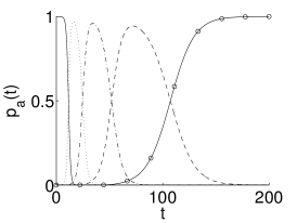
(a)

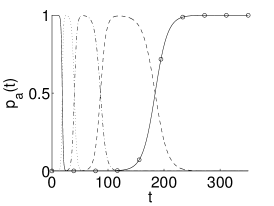
(b)

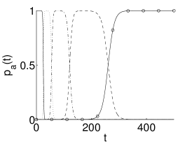
(c)

Figure B.2: Infinite population occupation numbers versus time for $k=4$, $r_{0}=0$, $r_{1}=1.00$, $r_{2}=1.45$, $r_{3}=1.65$, $r_{4}=1.74$, and three different values for $\mu$: (a) $10^{-5}$, (b) $10^{-8}$, and (c) $10^{-11}$. The occupation numbers, $p_{0}$ (solid), $p_{1}$ (dotted), $p_{2}$ (dash-dotted), $p_{3}$ (dashed), $p_{4}$ (solid with circles), are calculated using Eq. 12. Note that as $\mu$ becomes smaller, $p_{a}$ becomes more and more dominant during the time interval $t_{a}<t<t_{a+1}$.

Finally, the ratio of $p_{a+1}$ to $p_{a}$ is $\exp[\Delta r_{a+1}(t-t_{a+1})]\prod_{j=0}^{j=a-1}(r_{a}-r_{j})/(r_{a+1}-r_{j})$, which is small for $t<t_{a+1}$. Thus, for small $\mu$, in the time interval $t_{a}$ to $t_{a+1}$, most of the population is in state $a$. That is,

$$p_{a}(t)\gg p_{a^{\prime}}(t)\qquad a^{\prime}\neq a,t_{a}<t<t_{a+1},\mu\rightarrow 0.$$ (B.8)

Using this result and keeping the lowest order in $\mu$ in Eq. 22, we find

$$A_{ij}(t) \sim\left(r_{j}-r_{a}\right)\left(\delta_{i,j}-\delta_{i,a}\right),\qquad\qquad t_{a}<t<t_{a+1},\mu\rightarrow 0$$ (B.9)

such that

$$\frac{dC_{ij}(t)}{dt}\sim\bar{B}_{ij}(t)+\left(r_{i}+r_{j}-2r_{a}\right)C_{ij}(t)-\sum_{n}\left(r_{n}-r_{a}\right)\left(\delta_{j,a}C_{i,n}+\delta_{i,a}C_{j,n}\right).$$ (B.10)

For this landscape, Eq. B reduces to

$$\bar{B}_{ij}(t) =-\left[\mu\delta_{i,j-1}p_{i}(t)+\mu\delta_{i,j+1}p_{j}(t)+(r_{i}+r_{j})p_{i}(t)p_{j}(t)\right]$$

$$+\delta_{ij}\left(\mu p_{i-1}(t)+\mu\left(1-\delta_{i,k}\right)p_{i}(t)+r_{i}p_{i}(t)+\left<r\right>p_{i}(t)\right)$$ (B.11)

and, in particular,

$$\bar{B}_{kk}(t) =-2r_{k}\left(p_{k}(t)\right)^{2}+\mu p_{k-1}(t)+r_{k}p_{k}(t)+\left<r\right>p_{k}(t).$$ (B.12)

Substituting Eqs. B.1 and B.2 into this expression and keeping only the lowest power of $\mu$, we obtain, for $t<t_{1}$,

$$\bar{B}_{kk}(t<t_{1})\sim r_{k}\mu^{k}\sum_{a=0}^{k}\gamma^{k}_{a}e^{r_{a}t}\qquad\qquad\mu\rightarrow 0$$ (B.13)

and thus

$$\frac{dC_{kk}(t)}{dt}\sim r_{k}\mu^{k}\sum_{a=0}^{k}\gamma^{k}_{a}e^{r_{a}t}+2r_{k}C_{kk}(t),\qquad\qquad t<t_{1},\mu\rightarrow 0.$$ (B.14)

Integrating and only keeping terms to lowest order in $\mu$ yields

$$C_{kk}(t_{1})\sim\mu^{k}\left(\frac{\Delta r_{1}}{\mu}\right)^{2r_{k}/\Delta r_{1}}\sum_{a=0}^{k}\frac{\gamma^{k}_{a}}{2-r_{a}/r_{k}}\qquad\qquad\mu\rightarrow 0.$$ (B.15)

For later time periods, the evolution of $C_{kk}(t_{1}<t<t_{k})$ is dominated by the second term in Eq. B.10 as $\mu\rightarrow 0$:

$$\frac{dC_{kk}(t)}{dt}\sim 2\left(r_{k}-r_{a}\right)C_{kk}(t),\qquad\qquad t_{a}<t<t_{a+1},0<a<k,\mu\rightarrow 0$$ (B.16)

with solution

$$C_{kk}(t)\sim\mu^{k}e^{2(r_{k}-r_{a})t}\prod_{j=1}^{a}\left(\frac{\Delta r_{j}}{\mu}\right)^{2}\sum_{a^{\prime}=0}^{k}\frac{\gamma^{k}_{a^{\prime}}}{2-r_{a^{\prime}}/r_{k}}$$

$$t_{a}<t<t_{a+1},0<a<k,\mu\rightarrow 0.$$ (B.17)

Fig. B.3 shows the convergence of this approximation to Eq. 39 as $\mu\rightarrow 0$ for one set of replication rates.

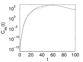
(a)

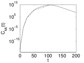
(b)

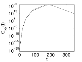
(c)

Figure B.3: Infinite population variance of the final state vs. time for $k=4$, $r_{0}=0$, $r_{1}=1.00$, $r_{2}=1.45$, $r_{3}=1.65$, $r_{4}=1.74$, and three different values for $\mu$: (a) $10^{-3}$, (b) $10^{-5}$, and (c) $10^{-8}$. Exact values calculated using Eq. 39 (solid lines) and the approximation given in Eq. B (dashed lines) are both shown. Note that $C_{kk}(t_{k})\propto\mu^{-k}$.

Using Eq. B, we find that as $\mu\rightarrow 0$

$$C_{kk}(t_{k}) \sim\mu^{k}e^{2\Delta r_{k}t_{k}}\sum_{a=0}^{k}\frac{\gamma^{k}_{a}}{2-r_{a}/r_{k}}\prod_{j=1}^{k-1}\left(\frac{\Delta r_{j}}{\mu}\right)^{2}$$

$$=\mu^{-k}\sum_{a=0}^{k}\frac{\gamma^{k}_{a}}{2-r_{a}/r_{k}}\prod_{j=1}^{k}\left(\Delta r_{j}\right)^{2}.$$ (B.18)

The maximum of $C_{kk}(t)$ occurs near $t_{k}$. This result follows from Eq. (B.10). The first term on the righthand side of Eq. (B.10) only matters during $0<t<t_{1}$. After that, $B_{kk}$ has a larger power of $\mu$ then $C_{kk}$ does. The second term on the righthand side is zero for $t>t_{k}$. Thus, for $t>t_{k}$, only the third term on the righthand side matters, and it is negative. Thus, for $t>t_{k}$, $C_{kk}(t)$ decreases. It is for this reason that the dashed curves in Fig. B.3 are shown for $0<t<t_{k}$ only.

Appendix C Fluctuations in the Expanded State Space at Large Times

Consider the expanded state space of a landscape as shown in Fig. 1 generalized to an arbitrary number of loci. For any finite population size $N$, the only sinks are the final states in which all mutations have occurred in some order, all of which have the same replication rate. Thus, after a certain time $t_{f}$, the occupation numbers at positions prior to the final states can be neglected so that the dynamics can be described by Eq. 2 with a single replication rate $r$ and without mutation,

$$\frac{\partial}{\partial t}P(\boldsymbol{N};t) =\frac{r}{N}\sum_{i,j\neq i}\left[\left(N_{i}-1\right)\left(N_{j}+1\right)P(\boldsymbol{N}-\boldsymbol{e}_{i}+\boldsymbol{e}_{j};t)-N_{i}N_{j}P(\boldsymbol{N};t)\right].$$

From this we obtain that the average occupation numbers remain constant

$$\left<N_{a}(t)\right>=\text{const}=\left<N_{a}(t_{f})\right>\qquad t\geq t_{f}$$ (C.1)

and that the covariances are

$$\Sigma_{ab}(t) \equiv\left<N_{a}(t)N_{b}(t)\right>-\left<N_{a}(t)\right>\left<N_{b}(t)\right>$$

$$=\left(1-e^{-2r(t-t_{f})/N}\right)\left<N_{a}\right>\left(\delta_{ab}N-\left<N_{b}\right>\right)+e^{-2r(t-t_{f})/N}\Sigma_{ab}(t_{f})\qquad t\geq t_{f}.$$ (C.2)

Expanding this to largest order in $N$, yields

$$\Sigma_{ab}(t)\sim 2r\left(t-t_{f}\right)\left(\delta_{ab}\left<N_{a}\right>-\frac{1}{N}\left<N_{a}\right>\left<N_{b}\right>\right)+\Sigma_{ab}(t_{f})\qquad t\geq t_{f}.$$ (C.3)

Note that the expansion in $N$ converges only for finite times.

References

[1]
H. J. Muller.
The relation of recombination to mutational advance.
Mutat. Res., 106:2–9, 1964.
[2]
W. G. Hill and A. Robertson.
The effect of linkage on limits to artificial selection.
Genetical Research, 8:265–294, 1966.
[3]
Michael M Desai and Daniel S Fisher.
Beneficial mutation selection balance and the effect of linkage on
positive selection.
Genetics, 176(3):1759–98, July 2007.
[4]
G. Sella and A. E. Hirsh.
The application of statistical physics to evolutionary biology.
Proc. Natl. Acad. Sci., 102:9541–9546, 2005.
[5]
J. Berg, S. Willmann, and M. Lässig.
Adaptive evolution of transcription factor binding sites.
BMC Evol. Biol., 4:42, 2004.
[6]
Philip Gerrish and Richard Lenski.
The fate of competing beneficial mutations in an asexual
population, 1998.
[7]
D Alves and J Fontanari.
Error threshold in finite populations.
Physical Review E, 57(6):7008–7013, June 1998.
[8]
P. A. P. Moran.
The Statistical Processes of Evolutionary Theory.
Clarendon Press, 1962.
[9]
Jeong-Man Park, Enrique Muñoz, and Michael W. Deem.
Quasispecies theory for finite populations.
Physical Review E, 81(1): 011902, 2010.
[10]
L. Peliti.
Path integral approach to birth-death processes on a lattice.
Journal de Physique, 46(9):1469–1483, 1985.
[11]
Colin J Thompson and John L McBride.
On Eigen’s theory of the self-organization of matter and the
evolution of biological macromolecules.
Mathematical Biosciences, 21(1-2):127–142, October 1974.
[12]
Kavita Jain, Joachim Krug, and Su-Chan Park.
Evolutionary advantage of small populations on complex fitness
landscapes.
Evolution; international journal of organic evolution,
65(7):1945–55, July 2011.
[13]
Matthew C. Cowperthwaite and Lauren Ancel Meyers.
How Mutational Networks Shape Evolution: Lessons from RNA Models.
Annual Review of Ecology, Evolution, and Systematics,
38(1):203–230, December 2007.
[14]
A B Bortz, M Kalos, and J Lebowitz.
A new algorithm for Monte Carlo simulation of Ising spin systems.
Journal of Computational Physics, 17(1):10–18, January 1975.
[15]
D Gillespie.
A general method for numerically simulating the stochastic time
evolution of coupled chemical reactions.
Journal of Computational Physics, 22(4):403–434, December
1976.
[16]
T. Paixão, D. M. Lorenz, J. Songhurst, M. W. Deem, R. Azencott, T. F.
Cooper, and R. B. R. Azevedo.
Clonal interference can lead to evolutionary farsightedness.
submitted.