Cold Fronts and Gas Sloshing in Galaxy Clusters with Anisotropic Thermal Conduction

Abstract

Cold fronts in cluster cool cores should be erased on short timescales by thermal conduction, unless protected by magnetic fields that are “draped” parallel to the front surfaces, suppressing conduction perpendicular to the sloshing fronts. We present a series of MHD simulations of cold front formation in the core of a galaxy cluster with anisotropic thermal conduction, exploring a parameter space of conduction strengths parallel and perpendicular to the field lines. Including conduction has a strong effect on the temperature distribution of the core and the appearance of the cold fronts. Though magnetic field lines are draping parallel to the front surfaces, preventing conduction directly across them, the temperature jumps across the fronts are nevertheless reduced. The geometry of the field is such that the cold gas below the front surfaces can be connected to hotter regions outside via field lines along directions perpendicular to the plane of the sloshing motions and along sections of the front which are not perfectly draped. This results in the heating of this gas below the front on a timescale of a Gyr, but the sharpness of the density and temperature jumps may be nevertheless preserved. By modifying the gas density distribution below the front, conduction may indirectly aid in suppressing Kelvin-Helmholtz instabilities. If conduction along the field lines is unsuppressed, we find that the characteristic sharp jumps seen in Chandra observations of cold front clusters do not form; therefore, the presence of of cold fronts in hot clusters is in contradiction with our simulations with full Spitzer conduction. This suggests that the presence of cold fronts in hot clusters could be used to place upper limits on conduction in the bulk of the ICM. Finally, the combination of sloshing and anisotropic thermal conduction can result in a larger flux of heat to the core than either process in isolation. While still not sufficient to prevent a cooling catastrophe in the very central ($r\sim$ 5 kpc) regions of the cool core (where something else is required, such as AGN feedback), it reduces significantly the mass of gas that experiences a cooling catastrophe outside those small radii.

1. Introduction

X-ray observations of galaxy clusters often show a bright, dense, centrally peaked core comprised of the intracluster medium (ICM) much cooler than the cluster average. The X-ray radiative cooling time, inversely proportional to the square of the gas density, is very short in these dense cores, on the order of several hundred Myr in the very central regions (Sarazin, 1986). This gave rise to an early “cooling flow” scenario, in which the gas cools catastrophically in the cluster center and is continuously replaced by the inflow of the surrounding cooling gas. However, Chandra and XMM-Newton have failed to detect the implied large quantities of very cool gas in the cores; in particular, the characteristic emission lines such as Fe XVII emitted by the plasma with $T<1$ keV are not observed (Peterson & Fabian, 2006). Since X-ray cooling is directly observed, a mechanism is required to heat the ICM in the core to compensate for the cooling. The two most studied heating mechanisms are feedback from active galactic nuclei (AGN) and thermal conduction. In this paper, we will be discussing the latter mechanism in connection with the phenomenon of gas sloshing.

The role of thermal conduction in the context of heating the cool cores of clusters of galaxies has been studied by many authors (see, e.g., Binney & Cowie, 1981; Narayan & Medvedev, 2001; Ruszkowski & Begelman, 2002; Zakamska & Narayan, 2003; Guo et al., 2008). Since in the ICM the Larmor radius of the electrons spiraling along the $B\sim 0.1-1$ $\mu$G magnetic field lines is many orders of magnitude smaller than the electron mean free path, the conduction is strongly anisotropic, occurring essentially exclusively along the field lines. Therefore, most of these works assumed an isotropically tangled magnetic field geometry and paramaterized the heat flux as an effective isotropic thermal conductivity given as a fraction, $f_{\rm Sp}$, of the ideal (field-free) Spitzer (1962) heat flux.

However, theoretical and numerical work over the last decade has revealed that the stability and thermal properties of the ICM are possibly more complicated than previously thought if anisotropic thermal conduction is modelled explicitly in the MHD regime. Early analysis by Balbus (2000, 2001) showed that when magnetized atmospheres with anisotropic thermal conduction are considered, their stability depends on the temperature gradient rather than the entropy gradient. He demonstrated that in regions where the temperature increases in the direction of gravity, the plasma is susceptible to the magnetothermal instability (hereafter MTI).

Further analytical work by Quataert (2008) and numerical work by Parrish & Quataert (2008) and Parrish et al. (2008, 2009) has shown that the cluster atmosphere is unstable even when the temperature decreases in the direction of gravity, as in the cluster cool cores (heat-flux buoyancy instability; HBI). The effect of the HBI is to realign the magnetic fields azimuthally $(\hat{\textbf{\emph{b}}}\cdot\hat{\textbf{\emph{{r}}}}\approx 0)$, and thereby significantly reduce the effective radial heat flux $Q_{r}$. This renders thermal conduction almost useless against preventing a “cooling catastrophe.” Subsequent work has shown that relatively low levels of turbulence can rearrange the field lines in a more isotropic configuration, permitting heat conduction to the core (Parrish et al., 2010; Ruszkowski & Oh, 2010, 2011). More recently, and of direct relevance to this work, Lecoanet et al. (2012) simulated the dynamics of Rayleigh-Taylor (RT) stable and unstable contact discontinuities with anisotropic thermal conduction. Of particular relevance is their finding that the temperature gradients of RT-stable contact discontinuities (such as sloshing cold fronts) can be smoothed by anisotropic thermal conduction if the field lines are at least partially misaligned with the surface of the discontinuity. The smoothing of the temperature gradient of the RT-stable contact discontinuities in these simulations was limited by the HBI, which reoriented magnetic field lines initially perpendicular to the front surface in a more parallel direction, suppressing conduction across the surface at later times.

So far, the numerical simulations of the evolution of the cluster atmospheres with anisotropic thermal conduction have mostly been limited to isolated, spherically symmetric clusters initially in hydrostatic equilibrium. These works have been essential in order to determine the character of the instabilities that are present when such physical effects are taken into account. A recent exception to this is the paper by Ruszkowski et al. (2011), which simulated the formation of a galaxy cluster from cosmological initial conditions.

The previous works assumed that the heat conduction along the field lines is at the Spitzer value. However, the effective conductivity along the field lines may be reduced due to strong curvature of the field lines and stochastic magnetic mirrors on small scales (e.g., Chandran et al., 1999; Malyshkin & Kulsrud, 2001; Narayan & Medvedev, 2001). Markevitch et al. (2003b) attempted to constrain heat conduction in the ICM from the observed temperature differences in the merging, non-cool-core cluster Abell 754. They determined that the effective conduction in the direction of the observed temperature gradients is an order of magnitude less than Spitzer, which, under the assumption of an isotropically tangled field, imples suppression along the field lines. Finally, Schekochihin et al. (2005) suggested that plasma microscale instabilities may be very important in the high-$\beta$ plasma of the ICM, and consequently its thermal conductivity may be many orders of magnitude smaller than the Spitzer value (Schekochihin et al., 2008).

In this work we consider a scenario where the initial cluster core is relaxed but undergoes a period of gas “sloshing.” Many cool-core systems exhibit edges in X-ray surface brightness approximately concentric with respect to brightness peak of the cluster (e.g., Mazzotta et al., 2001; Markevitch et al., 2001, 2003). X-ray spectra of these regions have revealed that in most cases the brighter (and therefore denser) side of the edge is the colder side, and hence these jumps in gas density have been dubbed “cold fronts” (for a detailed review see Markevitch & Vikhlinin, 2007). These features have been observed in the majority of cool-core systems (Ghizzardi et al., 2010). The presence of one or more cold fronts is seen as an indication of the motion of gas in a cluster. For relaxed systems, the primarily spiral-shaped cold fronts are believed to arise from gas sloshing in the deep dark matter-dominated potential well. These motions are initiated when the low-entropy, cool gas of the core is displaced from the bottom of the dark matter potential well, either by gravitational perturbations from infalling subclusters (Ascasibar & Markevitch, 2006) or by an interaction with a shock front (Churazov et al., 2003).

In an earlier paper, ZuHone et al. (2010, hereafter ZMJ10), we have investigated the possible flow of heat to the cluster cool core as a result of the sloshing motions bringing hot gas from larger radii into contact with the cool gas of the core. We determined that if the gas viscosity is small, significant mixing between the hot and cold gas will result, raising the entropy of the core, though this heat flow was found to be insufficient to completely offset the effects of radiative cooling. In that work, we did not include thermal conduction, but only mixing of gases with different temperatures.

ZMJ10 modeled the ICM as a (possibly viscous) unmagnetized fluid. However, the ICM is known to be magnetized, and this fact has important considerations for heat transport. For example, it has been suggested that the narrow width of cold fronts in galaxy clusters can be used to constrain the effectiveness of heat conduction in the ICM (e.g., Ettori & Fabian, 2000; Xiang et al., 2007). The sharp temperature gradient of the cold front should be smoothed out on short timescales if conduction is not suppressed across the front surface. Such suppression could be provided by magnetic field lines oriented parallel to the cold front surfaces, a situation believed to naturally arise due to the effects of magnetic draping and shear amplification (Asai et al., 2004, 2005; Lyutikov, 2006; Asai et al., 2007; Keshet et al., 2010). In a previous paper (zuh11, hereafter ZML11), we performed simulations of gas sloshing with magnetic fields, showing that such shear amplification and draping does occur around cold fronts in cluster cores. These simulations also showed that magnetic fields have similar effects as viscosity on the ICM, inhibiting the mixing of the hot and cold flows and reducing the increase of core entropy due to sloshing.

In this work, we build upon our earlier simulations (ZMJ10, ZML11) by including the effects of anistropic thermal conduction in a simulation of gas sloshing in a cool-core galaxy cluster. We will show that the magnetic fields draped across the cold fronts indeed inhibit the smoothing out of the temperature gradient, but only to a degree. The crucial points to note are a) due to fluid instabilities the magnetic field lines may not be oriented perfectly azimuthal with the front and b) cold fronts are not completely enclosed surfaces–there are still field lines that connect the cold side of the cold fronts to regions of higher temperature in the cluster atmosphere over short distances. Therefore, if thermal conduction is important, it may provide a more efficient way than gas mixing to transfer heat between the hot and cold flows characteristic of sloshing motions.

This paper is organized as follows: in Section 2 we describe the simulations and the code. In Section 3 we describe the effects of anisotropic conduction and gas sloshing on the thermal state of the cluster core for different configurations of the magnetic field and various prescriptions for thermal conduction. Finally, in Section 4 we summarize our results and discuss future developments of this work. We assume a flat $\Lambda$CDM cosmology with $h=0.7$, $\Omega_{\rm m}=0.3$, and $\Omega_{b}=0.02h^{-2}$.

2. Method

In our simulations, we solve the following set of MHD equations (in Gaussian units):

$$\frac{\partial{\rho}}{\partial{t}}+\nabla\cdot(\rho{\bf v}) = 0$$ (1)

$$\frac{\partial{(\rho{\bf v})}}{\partial{t}}+\nabla\cdot\left(\rho{\bf vv}-\frac{\bf BB}{4\pi}\right)+\nabla{p} = \rho{\bf g}$$ (2)

$$\frac{\partial{E}}{\partial{t}}+\nabla\cdot\left[{\bf v}(E+p)-\frac{{\bf B}({\bf v\cdot B})}{4\pi}\right] = \rho{\bf g\cdot v}-\nabla\cdot{\bf Q}$$

$$- n_{e}n_{H}\Lambda(T,Z)$$

$$\frac{\partial{\bf B}}{\partial{t}}+\nabla\cdot({\bf vB}-{\bf Bv}) = 0$$ (4)

where

$$p=p_{\rm th}+\frac{B^{2}}{8\pi}$$ (5)

$$E=\frac{\rho{v^{2}}}{2}+\epsilon+\frac{B^{2}}{8\pi}$$ (6)

where $p_{\rm th}$ is the gas pressure, $\epsilon$ is the gas internal energy per unit volume, and $\bf{B}$ is the magnetic field strength. For all our simulations, we assume an ideal equation of state with $\gamma=5/3$ and primordial abundances with molecular weight $\mu=0.6$.

We performed our simulations using FLASH 3.3, a parallel hydrodynamics/$N$-body astrophysical simulation code developed at the FLASH Center for Computational Science at the University of Chicago(Fryxell et al., 2000; Dubey et al., 2009). FLASH 3.3 solves the equations of magnetohydrodynamics using a directionally unsplit staggered mesh algorithm (USM; Lee & Deane, 2009). The USM algorithm used in FLASH 3.3 is based on a finite-volume, high-order Godunov scheme combined with a constrained transport method (CT), which guarantees that the evolved magnetic field satisfies the divergence-free condition (Evans & Hawley, 1988). In our simulations, the order of the USM algorithm corresponds to the Piecewise-Parabolic Method (PPM) of Colella & Woodward (1984), which is ideally suited for capturing shocks and contact discontinuties (such as the cold fronts that appear in our simulations).

The heat flux due to thermal conduction is given as:

$${\bf Q}=-\kappa_{\rm Sp}\left[f_{\perp}\left({\bf I}-\hat{\textbf{\emph{b}}}\hat{\textbf{\emph{b}}}\right)+f_{\parallel}\hat{\textbf{\emph{b}}}\hat{\textbf{\emph{b}}}\right]\cdot\nabla{T}$$ (7)

where we chose to represent the conductivity coefficient as a product of the Spitzer conductivity $\kappa_{\rm Sp}$ and the fractions $f_{\parallel}$ and $f_{\perp}$ of Spitzer conductivity parallel and perpendicular to the field line, respectively. $\hat{\textbf{\emph{b}}}\hat{\textbf{\emph{b}}}$ and ${\bf I}-\hat{\textbf{\emph{b}}}\hat{\textbf{\emph{b}}}$ are projection operators that single out the components of the temperature gradient $\nabla{T}$ parallel and perpendicular to the magnetic field line, with $\hat{\textbf{\emph{b}}}$ the unit vector in the direction of the local magnetic field. Most works assume $f_{\parallel}=1$ and $f_{\perp}=0$ in the conditions of the ICM (e.g., heat conducted strictly along the field lines without suppression), due to the large mean free path for collisions compared to the Larmor radius of the electron. We assume this prescription as the default, but also investigate alternative scenarios, represented by simulations with different values of $f_{\parallel}$ and $f_{\perp}$. For example, if the magnetic field is strongly curved on small scales, the effective conductivity along the field lines may be smaller than the Spitzer value, resulting in a smaller $f_{\parallel}$.

Alternatively, if a fraction of the magnetic field lines draped along the cold front surfaces reconnect with lines below these surfaces, a small amount of heat conduction perpendicular to the cold front surfaces may result. Our ideal MHD simulations do not model reconnection explicitly, as non-ideal terms including resistivity are not included (there is a small numerical resistivity associated with the finite resolution of the simulation, but this effective resistivity is negligible, see Section LABEL:sec:). However, we may account for the conduction that may occur across cold front surfaces in an approximate way by modeling it as a non-zero $f_{\perp}$, with the same temperature dependence as the parallel conduction. Since we are not modeling the reconnecting field lines and the conduction along them explicitly, our simple model is intended to provide only an order of magnitude estimate of this possible effect.

It is important to distinguish our ”perpendicular” conduction across the cold front surfaces from conduction perpendicular to the field lines resulting from collisions between electrons. Because the Larmor radius is many orders of magnitude smaller than the electron mean free path, this perpendicular conduction is effectively zero for the conditions in galaxy clusters. Additionally, the temperature dependence of this conduction would be $\propto T^{-1/2}$ instead of the $\propto T^{5/2}$ dependence for conduction along the field lines (Braginskii, 1965). In contrast, since our ”perpendicular” conduction is intended to account for conduction that occurs parallel to reconnecting field lines, it has the same temperature dependence as the parallel conduction.

Following Cowie & McKee (1977), we included the effect of conduction saturation whenever the characteristic lengthscale associated with the temperature gradient is smaller than the mean free path, though in the bulk of the ICM this effect is not significant. We implemented anisotropic conduction following the approach of Sharma & Hammett (2007). More specifically, we applied a monotonized central (MC) limiter to the conductive fluxes. This method ensures that anisotropic conduction does not lead to negative temperatures in the presence of steep temperature gradients. A verification test of our implementation of the anisotropic conduction module in FLASH 3.3 was given in Ruszkowski et al. (2011).

We want to examine the effects of anisotropic thermal conduction in a sloshing galaxy cluster core in isolation (in particular, the effect on the cold fronts), and so for most of our simulations, we do not include the effects of radiative cooling. We then include radiative cooling to determine the effect of sloshing with anisotropic conduction on the thermal state of the cluster core. The X-ray cooling function is determined using the Mewe, Kaastra, & Liedahl (1995) model with a uniform metallicity of $Z=0.3Z_{\sun}$.

The gravitational potential on the grid is set up as the sum of two “rigid bodies” corresponding to the contributions to the potential from both clusters. This approach to modeling the potential is used for simplicity and speed over solving the Poisson equation for the matter distribution, and is an adequate approximation for our purposes. It is the same approach that we used in ZML11, and is justified in Roediger & ZuHone (2011).

Table 1Simulation Parameter Space

Simulation	Relaxed/Sloshing	Magnetic Field	$f_{\parallel}$	$f_{\perp}$	X-ray Cooling?
S1	Sloshing	Tangled	0.0	0.0	NO
S2	Sloshing	Azimuthal	0.0	0.0	NO
SC1	Sloshing	Tangled	1.0	0.0	NO
SC2	Sloshing	Azimuthal	1.0	0.0	NO
SC3	Sloshing	Tangled	0.1	0.0	NO
SC4	Sloshing	Tangled	0.1	0.01	NO
RX	Relaxed	Tangled	0.0	0.0	YES
RCX	Relaxed	Tangled	1.0	0.0	YES
SX	Sloshing	Tangled	0.0	0.0	YES
SCX1	Sloshing	Tangled	1.0	0.0	YES
SCX2	Sloshing	Azimuthal	1.0	0.0	YES
SXNoB	Sloshing	No Fields	0.0	0.0	YES

We refer the reader to ZML11 for the full details of our physical setup, but will provide the following short description. Our simulations consist of a massive ($M\approx 1.5\times 10^{15}{\cal M}_{\sun}$, $T_{X}\sim 8$ keV), cool-core cluster, initially in hydrostatic equilibrium, merging with a small (mass ratio $R$ = 5) gasless subcluster, which sets off the sloshing of the cool core. We begin the simulation at a point in time when the cluster centers have a mutual separation of $d$ = 3 Mpc and an impact parameter $b$ = 500 kpc. The initial velocities of the subclusters are set up assuming that the total kinetic energy of the system is set to half of its total potential energy. For all of the simulations, we set up the main cluster within a cubical computational domain of width $L=2.4$ Mpc on a side, with a finest cell size on our AMR grid of $\Delta{x}=2.34$ kpc.

The magnetic field of the cluster is set up in an identical way to the simulations of ZML11, following the approach of Ruszkowski et al. (2007, 2008) and Ruszkowski & Oh (2010). A random magnetic field $\tilde{\bf B}({\bf k})$ is set up in $\bf{k}$-space on a uniform grid using independent normal random deviates for the real and imaginary components of the field. Thus, the components of the complex magnetic field in $\bf{k}$-space are set up such that

$$\tilde{B_{x}}(\bf{k}) = B_{1}[N(u_{1})+iN(u_{2})]$$ (8)

$$\tilde{B_{y}}(\bf{k}) = B_{2}[N(u_{3})+iN(u_{4})]$$ (9)

$$\tilde{B_{z}}(\bf{k}) = B_{3}[N(u_{5})+iN(u_{6})]$$ (10)

where $N(u)$ is a function of the uniformly distributed random variable $u$ that returns Gaussian-distributed random values, and the values $B_{i}$ are field amplitudes. We adopt a dependence of the magnetic field amplitude $B(k)$ on the wavenumber $|\bf{k}|$ similar to (but not the same as) Ruszkowski et al. (2007) and Ruszkowski & Oh (2010):

$$B(k)\propto k^{-11/6}{\rm exp}[-(k/k_{0})^{2}]{\rm exp}[-k_{1}/k]$$ (11)

where $k_{0}$ and $k_{1}$ control the exponential cutoff terms in the magnetic energy spectra. The cutoff at high wavenumber $k_{0}$ roughly corresponds to the coherence length of the magnetic field $k_{0}=2\pi/\lambda_{0}=2\pi/(43~{}{\rm kpc})$, observed in some cluster cores. The cutoff at low wavenumber $k_{1}=2\pi/\lambda_{1}$ roughly corresponds to $\lambda_{1}\approx r_{500}/2\approx$ 500 kpc, which is held fixed for all of our simulations. This field spectrum corresponds to a Kolmogorov shape for the energy spectrum $(P_{B}(k)\propto k^{-5/3})$ with cutoffs at large and small linear scales. This field is then Fourier transformed to yield ${\bf B}({\bf x})$, which is rescaled to have an average value of $\sqrt{8\pi{p}/\beta}$ to yield a field with a pressure that is proportional to the gas pressure, i.e., to have a spatially uniform $\beta$ for the initial field. We set the initial $\beta=400$. This procedure ensures that there will be significant power at all length scales between $\lambda_{1}$ and $\lambda_{0}$, which will result in a field that is significantly tangled down to the scale of $\lambda_{0}$.

As mentioned above, previous simulation works have predicted that due to the action of the HBI, an azimuthal magnetic field should arise in the cluster core, in the absence of turbulence driven by galaxy motions or AGN. For this purpose, we also include a simulation that has a purely azimuthal initial field similar to that used in Bogdanović et al. (2009), described in spherical coordinates by

$$B_{r} = 0$$ (12)

$$B_{\theta} = 2B_{0}\sin{\theta}\cos{2\phi}$$ (13)

$$B_{\phi} = -B_{0}\sin{2\phi}\sin{2\theta}$$ (14)

Its magnitude was then scaled by the gas pressure with $\beta=400$.

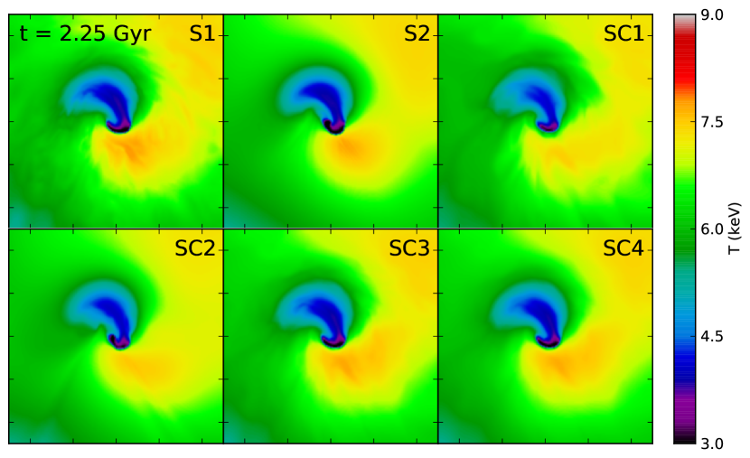
Figure 1.— Slices through the center of the domain in the $x-y$ plane of the temperature for the sloshing simulations with and without conduction for the epoch $t$ = 2.25 Gyr. Each panel is 500 kpc on a side. The colorscale is temperature in keV. Major tick marks indicate 100 kpc distances.

Finally, for both configurations, a field consistent with $\nabla\cdot{\bf B}=0$ is generated by performing the Fourier transform and then by “cleaning” the field of divergence terms in Fourier space via the the projection

$$\tilde{\bf B}^{\prime}({\bf k})=(\bf{I}-\bf{\hat{k}\hat{k}})\tilde{\bf B}({\bf k})$$ (15)

where $\hat{\bf{k}}$ is the unit vector in $\bf{k}$-space, and I is the identity operator. Note that this operation does not change the power spectrum of the magnetic field fluctuations. Upon transformation back to real space, the magnetic field satisfies $\nabla\cdot{\bf B}=0$. This field is then interpolated onto our AMR grid in such a way that the condition $\nabla\cdot{\bf B}=0$ is maintained.

Because our sloshing simulations begin with the two clusters at a distance, it takes a period of time ($\sim$2 Gyr) for the influence of the subcluster to perturb the cool core of the main cluster and initiate sloshing. If we had began the simulation with anisotropic thermal conduction “switched on”, it would alter the thermal state of the core and the HBI and MTI would alter the cluster magnetic field spatial configuration long before sloshing had begun, since the growth times of these instabilities and the conduction timescale for the core are on the order of $\sim$ a few $10^{8}$ yr. Worse yet, if we began the simulation with radiative cooling switched on, the cool core would cool rapidly (also on a timescale of $\sim$ a few $10^{8}$ yr) and we would have a cooling catastrophe before sloshing started. To avoid these effects, we switch on conduction (and cooling in the simulations where it is included) at a time $t\sim 2$ Gyr after the beginning of the simulation, shortly after the subcluster has made its pericentric passage of the cluster core and right at the beginning of the sloshing period. This enables us to examine the effects of conduction and sloshing together on a typical cool-core cluster state.

An unfortunate side-effect of this evolutionary period before the core passage is that the magnetic field configuration will slowly evolve away from its initial configuration. Hence, the initially isotropically tangled field configuration with $\langle|\hat{\textbf{\emph{b}}}\cdot\hat{\textbf{\emph{{r}}}}|\rangle=0.5$ evolves to a slightly more radial field configuration with $\langle|\hat{\textbf{\emph{b}}}\cdot\hat{\textbf{\emph{{r}}}}|\rangle\approx 0.56$, and the initially azimuthal field configuration with $\langle|\hat{\textbf{\emph{b}}}\cdot\hat{\textbf{\emph{{r}}}}|\rangle=0$ also evolves to a slightly more radial field configuration with $\langle|\hat{\textbf{\emph{b}}}\cdot\hat{\textbf{\emph{{r}}}}|\rangle\approx 0.35$. This is not a major concern, as the former is not too far off from an isotropically tangled field configuration and the latter is not too far from the field configuration of the saturation state of the HBI as seen in simulations (Parrish et al., 2009; Bogdanović et al., 2009). In real clusters, there is always turbulence and small disturbances from galaxies and DM clumps that keep the field tangled (Parrish et al., 2010; Ruszkowski & Oh, 2010, 2011).

We will refer to the simulations using the following codes. The letter “R” will indicate a cluster that is evolved in isolation, whereas “S” will indicate a cluster evolved with a gravitational interaction causing sloshing. “C” will indicate anisotropic thermal conduction is turned on, and “X” will indicate X-ray radiative cooling is turned on. Simulations that differ in the prescription for conduction and the initial field line configuration will be delimited by numbers. Table 1 lists all simulation runs with their particular parameters.

3. Results

3.1. Brief Outline of the Sloshing Process

We have described the initiation and the evolution of sloshing cold fronts in previous works (e.g., AM06, ZMJ10, ZML11), the latter paper including the effects of magnetic fields. We refer the reader to these papers for the full description, but we will outline the process in brief here.

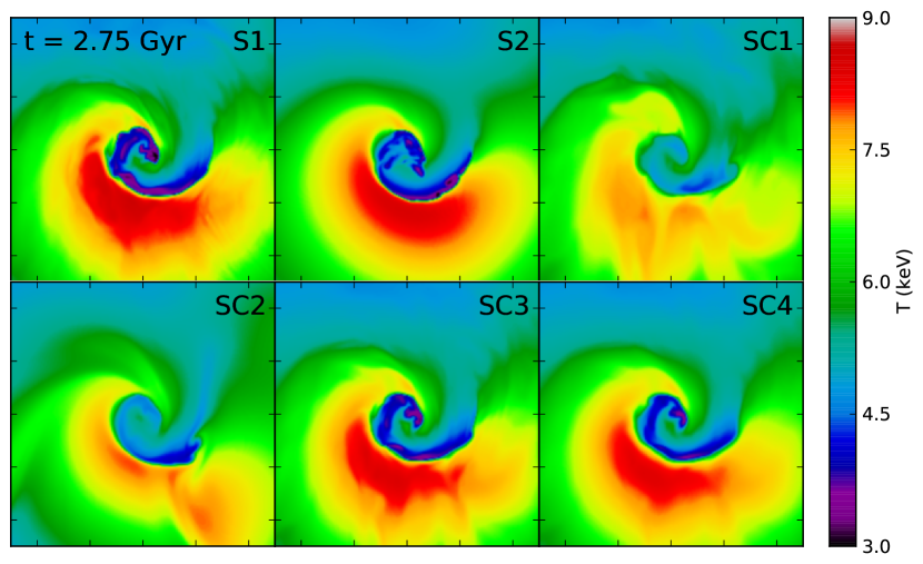
Figure 2.— Same as Figure 1 but corresponding to the epoch $t$ = 2.75 Gyr.

As the subcluster approaches the main cluster’s core and makes its passage, the gas and DM peaks of the main cluster feel the same gravity force toward the subcluster and move together towards it. However, the gas feels the effect of the ram pressure of the ambient medium. This fact becomes significant as the gas core is held back from the core of the dark matter by this pressure. This results in a separation of the gas and DM peaks of the cluster. As this ram pressure declines with the decreasing gravitational attraction of the outgoing subcluster, the gas that was held back by the ram pressure falls into the DM potential minimum and overshoots it. In addition to the gravitational disturbance, the wake trailing the subcluster transfers some of the angular momentum from the subcluster to the core gas and also helps to push the core gas out of the DM potential well. As the cool gas from the core climbs out of the potential minimum, it expands adiabatically. However, the densest, lowest-entropy gas quickly begins to sink back towards the potential minimum against the ram pressure from the surrounding ICM. Once again, as the cool gas falls into the potential well it overshoots it, and the process repeats itself on a smaller linear scale. Each time, a contact discontinuity (“cold front”) is produced. Due to the angular momentum transferred from the subcluster by the wake, these fronts have a spiral-shaped structure. As we noted in ZML11, this general outline is not affected significantly by the strength of the magnetic field or its spatial configuration, so the features seen in density and temperature maps are essentially the same between our two reference (e.g., without conduction) simulations, S1 and S2 (the S1 simulation corresponds to the Beta400 simulation in ZML11), and the runs without magnetic fields in ZMJ10. When speaking of the orientation of the temperature gradient across the cold fronts, we shall refer to the hotter, less dense gas as the side “above” the front and the colder, denser gas “below” the front, consistent with the direction of the gravitational acceleration.

3.2. The Effect of Conduction on Cold Fronts

Figures 1 through 4 show slices through the center of the cluster of the gas temperature for several different epochs, for our simulations with and without anisotropic conduction (but without radiative cooling). We will first compare runs with no conduction to runs with full Spitzer conduction along the field lines ($f_{\parallel}=1,f_{\perp}=0$). Our runs S1 (top left panels) and S2 (top center panels) correspond to sloshing simulations with initially tangled fields and initially azimuthal fields, respectively. Likewise, our runs SC1 (top right panels) and SC2 (bottom left panels) correspond to sloshing simulations with anisotropic heat conduction, with initially tangled fields and initially azimuthal fields.

Including conduction has a dramatic effect on the temperature structure of the cold fronts. The adiabatic simulations without conduction (S1 and S2) develop a number of well-defined cold fronts over time, which maintain temperature differences of $\sim$1.5-2 across the fronts throughout their evolution. This is not the case for the simulations with anisotropic unsuppressed Spitzer conduction (simulations SC1 and SC2). Over time, the cold gas inside the fronts is heated up, so that the temperature contrasts across the fronts become smaller, roughly $\sim$1.3-1.5. The changing thermal state of the gas also changes the shape of the fronts in some places. In particular, due to the fact that the inner 50 kpc becomes nearly isothermal, cold fronts do not occur on the smallest scales, in conflict with observations of cool-core clusters, which typically show a number of cold fronts at both small and intermediate radii within the core. The temperature of the core in simulation SC2 increases more slowly than in simulation SC1, because the more azimuthally oriented field lines in the former suppress conduction from larger radii more efficiently than the more tangled fields of simulation SC1 do.

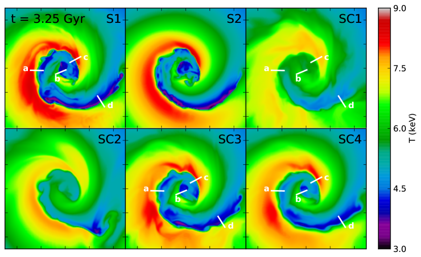
Figure 3.— Same as Figure 1 but corresponding to the epoch $t$ = 3.25 Gyr. The profiles marked with letters correspond to those plotted in Figures 5 and 6.

Figures 1 through 4 also show results for the simulations with other values for the conduction coefficients $f_{\perp}$ and $f_{\parallel}$. The SC3 simulation has the same field line configuration as the SC1 simulation, but the conduction along the lines is suppressed by a factor of 10. If field lines are strongly curved on very small linear scales, the effective conduction coefficient parallel to the field lines may be smaller than the Spitzer value by an order of magnitude due to the presence of stochastic magnetic mirrors (e.g., Narayan & Medvedev, 2001). We choose $f_{\parallel}=0.1$ to determine the effect of such a reduction. Alternatively, if plasma microscale instabilities play a significant role, the thermal conductivity of the ICM may be many orders of magnitude smaller (Schekochihin et al., 2008). For all practical purposes, this case is equivalent to the runs without conduction.

On the other hand, if (for example) $\sim$1% of the magnetic field lines parallel to the fronts reconnect, the effective fraction of Spitzer conduction perpendicular to the large-scale direction of the field could be $f_{\perp}\sim 0.01$. We assume this value of $f_{\perp}$ for simulation SC4, keeping the value of $f_{\parallel}=0.1$ for comparison with simulation SC3. As expected, for the SC3 simulation, far less heat is conducted to the cluster core, and the temperature contrast of the cold fronts with the surrounding medium is much closer to the case without any conduction. In the SC4 simulation, the small perpendicular conductivity, combined with a steep temperature jump across the cold front, has succeeded over time to smooth out the temperature gradient across the cold fronts.

Figure 5 compares temperature gradients across cold fronts between the S1 and the SC1 simulations at a late epoch, $t$ = 3.25 Gyr. Four particular locations across the fronts are picked out for inspection (see Figure 3 for the profile locations, marked by the corresponding letters). The profiles show that the temperature jumps in the conducting simulation have all been reduced. For some of the profiles (e.g., (a) and possibly (d)), the width of the temperature jump in the simulation with conduction SC1 is not greater than the jump in the non-conducting simulation S1 (a few simulation cells, $\sim 5-10$ kpc–essentially unresolved by the simulations), whereas for other profiles in simulation SC1, the temperature jumps have been smoothed out over several zone sizes (we will explore these issues further in Section 3.3). Particularly apparent in profile (d) is that conduction has modified the temperature distribution below the front, while preserving the sharp jump across the front.

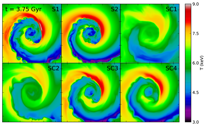
Figure 4.— Same as Figure 1 but corresponding to the epoch $t$ = 3.75 Gyr.

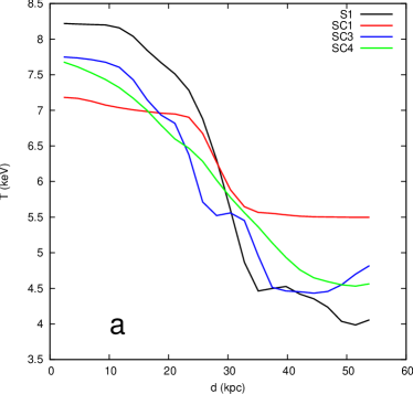
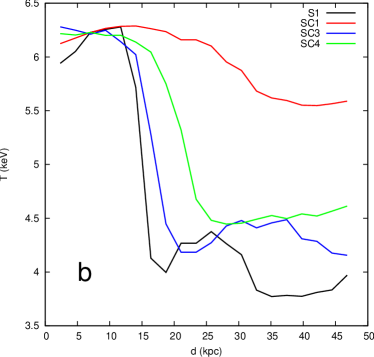
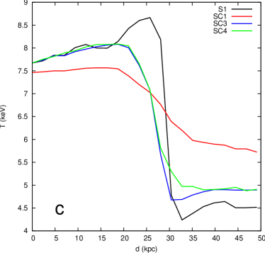
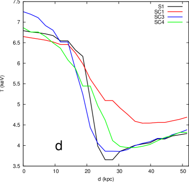
Figure 5.— Temperature profiles of cold fronts in simulations without conduction and with varying prescriptions for conduction, along the profiles marked with the corresponding letters in Figure 3. Conduction reduces the magnitude and increases the width of the jumps to varying degrees.

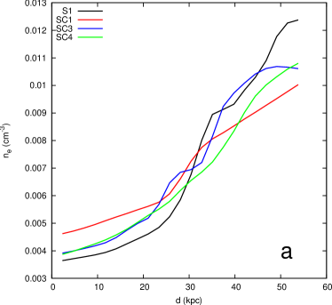
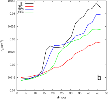
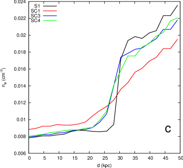
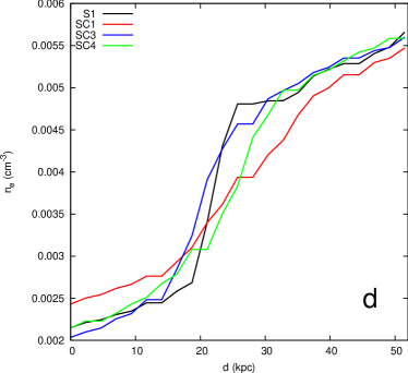
Figure 6.— Density profiles of cold fronts in simulations without conduction and with varying prescriptions for conduction, along the profiles marked with corresponding letters in Figure 3.

Figure 5 also highlights example temperature jumps in the SC3 and SC4 simulations (along the same profile locations, see Figure 3). The temperature difference across the fronts are similar between these two simulations and the S1 simulation, due to the high suppression of conduction, but the smoothing out of the gradient due to the conduction perpendicular to the field lines in the SC4 simulation is noticeable, with the temperature change occurring over roughly twice the number of cells ($\sim$10 kpc) compared to the case without perpendicular conduction due to field line reconnection.

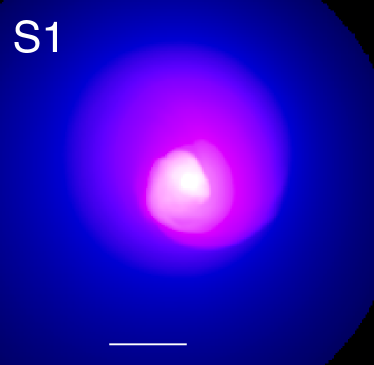
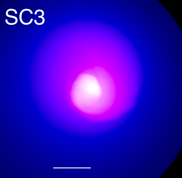
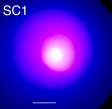
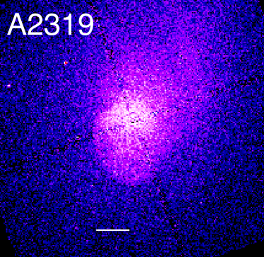
Figure 7.— Projected X-ray emission along the $z$-axis of the simulation domain for the S1 (no conduction), SC1 (Spitzer conduction), and SC3 (0.1 Spitzer conduction) simulations at the epoch $t$ = 2.75 Gyr, with a Chandra X-ray image of A2319 included for comparison. White bars indicate 100 kpc distances. This indicates that conduction smooths out the density jumps, making them barely discernable as seen in X-ray images in comparison to the sharp jumps in emission seen in A2319.

The jumps in density across the cold fronts are similarly affected by conduction. As heat flows from the hot gas above the cold fronts to the cool gas below the front, the former contracts and the latter expands in the same proportion as the change in temperature. Figure 6 shows the density jumps across the cold fronts at the same positions in Figure 3. In simulations with conduction, the density jumps are reduced and the widths of the density jumps are increased to varying degrees, in the same proportion as the temperature jumps except that the sign of the gradient is reversed. In the most extreme cases, the density jumps have been essentially erased, either in the strong parallel conduction case SC1 or the case SC4 with a small component of conduction perpendicular to the magnetic field lines. The smoothed profiles in these simulations are in disagreement with observations of cold fronts in clusters.

The differences between the simulations S1, SC3, and SC4 indicate that numerical reconnection across the cold front surfaces and any associated heat flux due to this reconnection is negligible. The cold fronts in the simulations S1 and SC3 have essentially the same temperature and density jumps, whereas adding a small perpendicular conduction smooths out the jumps over twice the number of cells. The fact that we do not see this degree of smoothing in the SC3 simulation indicates that numerical reconnection is too small to provide any significant heat flux across the fronts.

The smaller density jumps and the modification of the density profiles below the fronts that reduce the density contrast have a significant effect on the appearance of cold fronts as seen in X-ray images, due to the strong dependence of the X-ray emission on the gas density. Figure 7 shows synthetic X-ray images for the S1, SC1, and SC3 simulations, at the epoch $t$ = 2.75 Gyr, created by computing the bolometric MeKaL emissivity in each FLASH cell and projecting it along the $z$-axis (in the same manner as ZML11). Additionally, a Chandra X-ray image of Abell 2319 is also presented for comparison (this cluster is slightly hotter than our model cluster, with average $T\sim 9-10$ keV). This cluster exhibits a cold front with a very sharp jump in X-ray emission, with a width roughly the size of the Chandra PSF (O’Hara et al., 2004; Govoni et al., 2004).

The characteristic spiral shape of the cold fronts is apparent in each simulated image. However, the sharp edges in emission across the front surfaces are essentially absent from the SC1 case, whereas in the SC3 and S1 simulations, the sharp jumps are clearly seen. Therefore, for our simulated hot cluster, unsuppressed Spitzer conduction appears to produce cold fronts that are far less prominent than those in observed hot clusters, and it is questionable whether or not they may be even called “cold fronts” at all. We reserve a more quantitative comparison with observed clusters of different temperatures and plasma $\beta$ values and the possible constraints on conductivity for a future paper.

It also is apparent from these figures that conduction may have an effect on the smoothness of the front surfaces. For example, the cold fronts in simulations SC1 and SC2 exhibit fewer small-scale features along the front surfaces than their counterparts without conduction, S1 and S2. The widening of the cold front interfaces (seen clearly in Figure 6) will cause them to be less susceptible to the Kelvin-Helmholtz instability (see, e.g., Churazov & Inogamov, 2004).

3.3. The Geometry of the Magnetic Field Lines

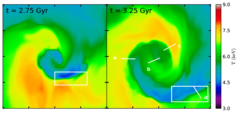
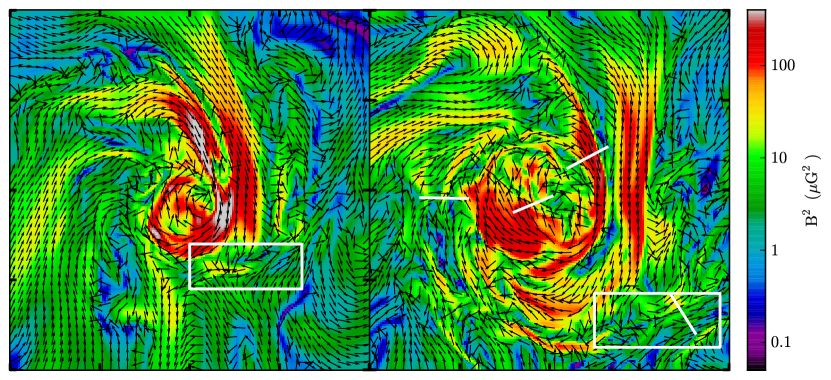
Figure 8.— Slices through the $z$ = 0 coordinate plane of the temperature and the magnetic field energy in the vicinity of four representative profiles with the 2D vector field $\hat{\textbf{\emph{b}}}=(b_{x},b_{y})$ overlaid for the simulation SC1 (Spitzer conduction along field lines) at the epochs $t$ = 2.75 Gyr and 3.25 Gyr. Each panel is 400 kpc on a side. Tick marks indicate 100 kpc distances. The field vectors are located at the positions of their tails. Top panels: Temperature in keV. Bottom panels: The magnetic field energy $B^{2}$ in $\mu{G}^{2}$. Red, elongated regions in the bottom panels indicate magnetic draping layers. The white rectangles indicate the regions without strong draping layers described in the text. The white lines indicate the profile locations from Figure 3.

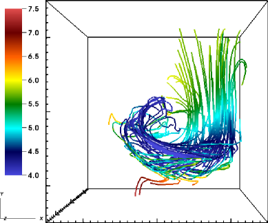
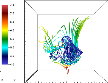
Figure 9.— Magnetic field lines in the SC1 (Spitzer conduction) simulation beginning at points inside the cold fronts with $T<$ 4.5 keV and continuing up to a length of 100 kpc at the epoch $t$ = 2.5 Gyr. Left panel: View along the $z$-axis. Right panel: View along the $x$-axis. Color along the lines indicates temperature in keV. The box size is 150 kpc, and the major tick marks indicate 50 kpc distances. This indicates that field lines connect regions of cold gas under the cold front surfaces to hot gas outside them.

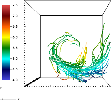
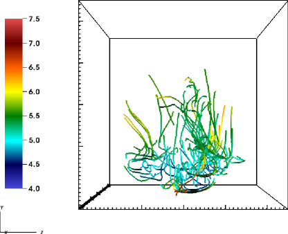
Figure 10.— Magnetic field lines in the SC1 simulation beginning at points inside the cold fronts with $T<$ 5.5 keV and continuing up to a length of 100 kpc at the epoch $t$ = 3.0 Gyr. Left panel: View along the $z$-axis. Right panel: View along the $x$-axis. Color along the lines indicates temperature in keV. The box size is 250 kpc, and the major tick marks indicate 50 kpc distances. This indicates that field lines connect regions of cold gas under the cold front surfaces to hot gas outside them.

The simulations from ZML11 showed magnetic field is amplified and the lines oriented parallel to the cold front surfaces, which would prevent conduction across the cold front surfaces from the hotter gas just above the fronts. The fact that there are examples of discernable temperature jumps over the same spatial range (a few simulation cells) even in the SC1 run indicates that conduction is still strongly suppressed directly across the front surfaces. What accounts for the significant changes in density and temperature across the fronts that still occur?

Figure 11.— The evolution of the volume-averaged (within a sphere of radius $R$ = 100 kpc) angle between the magnetic field unit vector and the radial unit vector $\langle\theta_{B}\rangle=\cos^{-1}\langle|\hat{\textbf{\emph{b}}}\cdot\hat{\textbf{\emph{{r}}}}|\rangle$ over time for simulations with and without conduction.

The cool gas below the cold fronts is only completely immune to the effects of heat conduction if there are no field lines leading from hotter regions of the cluster atmosphere into the cold regions of the fronts from other directions. The fronts seen in X-ray observations do not completely enclose the cool core. In principle, there could be magnetic field lines that reach the regions below the fronts from hotter regions on the other side of the cluster. More importantly, simulations of gas sloshing show that the resulting spiral structure has an alternating pattern of hot and cold flows, with hot flows developing below cold fronts as they expand to higher radii. Keshet (2011) showed that these latter flows are of hot gas being drawn into the core region form higher radii. These regions can be magnetically connected to the cool gas immediately below the fronts. Additionally, though the cold fronts that form in simulations are extended in directions perpendicular to the sloshing plane, the characteristic size of the fronts in this direction (along the line of sight where the observer sees the spiral structure) is smaller than in the plane. This exposes the cold regions of the fronts to magnetic field lines extending into hotter regions along directions perpendicular to the sloshing plane.

The preceding arguments lead us to expect that some field lines that pass through cold gas below the front surfaces may be connected to hotter regions over relatively short distances. Figures 9 and 10 show magnetic field lines beginning at several points in the cold region below the front surface and followed for a distance of 100 kpc. A large number of field lines are tangentially oriented to the front surfaces, as can be easily seen in both projections, shielding this cold gas from the hotter gas directly above the front. However, the figures show that there are still a number of field lines that extend into hotter regions of the cluster core along other directions. At the epochs of $t$ = 2.5 Gyr and $t$ = 3.0 Gyr, the coldest temperatures below the front surfaces are approximately $T\sim$4.5-5 keV, and these regions are connected to regions with temperatures of $T\sim$6-7.5 keV. In the right panel of Figure 9, field lines stretched along the $y$ and $z$ directions connect cold gas underneath the front surfaces to hotter gas. In Figure 10, lines connecting cool gas with hot gas that was brought in by sloshing are evident near the center of the left panel of the figure.

Finally, the simulations show that there is not always a perfect alignment of strong magnetic field layers with cold fronts. Figure 8 shows slices through the center of the simulation domain in the $x-y$ plane (coincident with the plane of the sloshing motions) of the gas temperature and the magnetic field energy for the epochs $t$ = 2.75 Gyr and $t$ = 3.25 Gyr with the magnetic field vector components in the $x$ and $y$-directions overlaid. Extended regions of strong magnetic field indicate places where the magnetic field strength has been increased by shear amplification. The locations of the profiles from Figure 3 are also marked. While some locations along the cold fronts exhibit a strong field layer parallel to the front, this is not strictly true everywhere along the fronts. In particular, the $t$ = 2.75 Gyr panel shows that the trailing edge of the cold spiral in the southwestern direction (indicated roughly by the white rectangles in Figure 8) is not draped by a high-$B$ layer. It can be seen that the magnetic field vectors along this portion of the spiral front are not strictly aligned parallel to the front surface. Regions of ordered, strong field are interspersed with regions of weak, tangled field as shown by the vectors at these locations. At a somewhat later time, $t$ = 3.25 Gyr, this location still lacks a strongly magnetized parallel layer. This also happens to be the location of profile (d). That particular temperature jump was shown to be smoothed out significantly in Figure 5. Though at the epoch $t$ = 3.25 Gyr there does appear to be a small, parallel, highly magnetized layer at that particular front location, this layer was not present previously and the temperature jump likely has been smoothed out before the formation of this layer.

Cold fronts that are not draped by strong magnetic fields will be more susceptible to the K-H instability, which will distort the front surface and lead to gas mixing between hot and cold phases. This is because the orientation of the draping fields tends to coincide with the direction of the shearing motions. Perturbations of the field lines perpendicular to the front surfaces at these locations will lead to smoothing out of the fronts as outlined in Lecoanet et al. (2012), though the extent of this smoothing will be limited by the HBI, which will reorient magnetic field lines parallel to the front surface. Lecoanet et al. (2012) estimated that the scale height of the temperature gradient for such a front would smooth to a height of $h_{T}\sim\chi^{2/3}/g^{1/3}$, where $\chi$ is the Spitzer thermal diffusivity and $g$ is the gravitational acceleration. Taking example values from our simulation for a cold front at $r\approx$120 kpc, we find $\chi\sim 5\times 10^{30}$ cm² s^-1 and $g\sim 3\times 10^{-8}$ cm s^-2. This yields an approximate scale height of the temperature gradient across the front of $h_{T}\sim 30$ kpc, which is similar to the widths of some of the temperature gradients across the fronts in Figure 5.

In simulations of thermal instabilities in magnetized galaxy clusters, a helpful quantity to examine has been the average angle between the magnetic field and radial unit vectors, given by

$$\langle\theta_{B}\rangle=\cos^{-1}\langle|\hat{\textbf{\emph{b}}}\cdot\hat{\textbf{\emph{{r}}}}|\rangle$$ (16)

Isotropically oriented tangled field lines will have an average $\langle|\hat{\textbf{\emph{b}}}\cdot\hat{\textbf{\emph{{r}}}}|\rangle=0.5$ and hence the corresponding angle is $\langle\theta_{B}\rangle\approx 60^{\circ}$. The HBI drives field lines in a more azimuthal direction ($\theta_{B}\sim 70-80^{\circ}$) in the presence of a positive radial temperature gradient (as in a cool core). Sloshing motions in general preserve the overall positive temperature gradient of the cool core, implying that the HBI should still be active. However, they will also drag the field lines around into a more azimuthally oriented configuration as they are draped around the cold fronts.

Figure 11 shows the evolution of the volume-averaged angle of the magnetic field with respect to the radial direction within a radius of 100 kpc over time for the S1, S2, SC1, and SC2 simulations. The simulations with initially tangled and azimuthal fields begin with $\langle\theta_{B}\rangle\approx 56^{\circ}$ and $\langle\theta_{B}\rangle\approx 70^{\circ}$, respectively. We find that largely the evolution of this “magnetic angle” is driven by the sloshing motions themselves, since the evolution of $\theta_{B}$ is essentially identical between the simulations with and without conduction that have the same initial magnetic field setup. An exception to this general rule are the simulations with initially azimuthal magnetic field lines, S2 and SC2. When conduction is included, the final $\theta_{B}$ indicates a more azimuthal direction than in the case where conduction is absent. This is possibly due to the fact that in this case the core is more magnetically isolated due to the azimuthally oriented field lines, and the positive temperature gradient is better preserved in the core than in the tangled field line case. In such a scenario, the HBI would drive the field lines in a more azimuthal direction once the conduction is turned on.

3.4. The Evolution of the Entropy of the Cluster Core

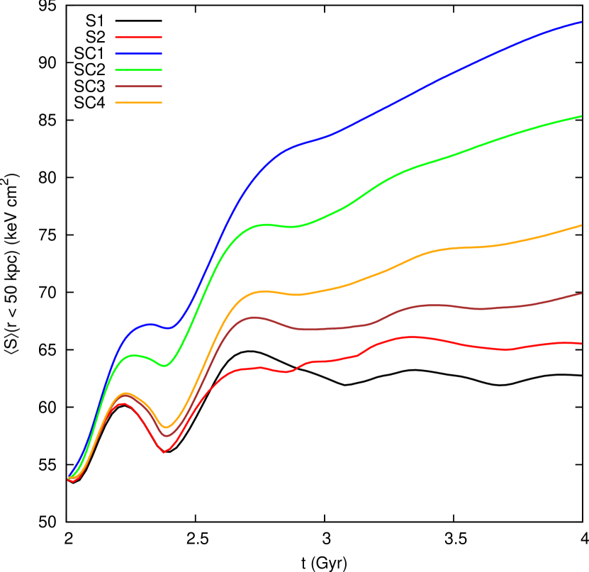
Figure 12.— Evolution of the average entropy within 50 kpc of the cluster center for simulations with and without anisotropic thermal conduction.

Given that our simulations show that the magnetic field geometry of the sloshing cool core still permits heat conduction to the cluster core, it is important to determine what effect this has on the thermal state of the core. The evolution of average entropy within the inner 50 kpc of the cluster center over time is shown in Figure 12. In the simulations without conduction (S1 and S2), the average entropy of the cluster core increases due to sloshing bringing hot gas from the cluster outskirts with the cool gas of the core into contact, which then mix to a certain degree. However, the magnetic field suppresses such mixing (ZML11), and the increase in entropy levels off roughly 0.5 Gyr after the simulation begins. ZML11 showed that the difference in initial field geometry has little effect on the entropy increase in this case.

In contrast, in the simulations with anisotropic Spitzer conduction (SC1 and SC2), heat conducts along the field lines to the cluster center, and the entropy increase of the core continues unabated for the duration of the simulation. As expected, the effect is stronger in the case with initially random field lines than in the case with initially azimuthal field lines. The average specific entropy increase in these two simulations is roughly $\Delta{S}\sim 20-30$ keV cm² higher than in the adiabatic simulations.

A similar situation exists for the simulations with weaker conduction coefficients. The simulation with conductivity 1/10 of the Spitzer value strictly along the field lines (SC3) has a correspondingly smaller increase in entropy over the SC1 simulation, with $\Delta{S}\sim 5$ keV cm², close to the entropy increase due to sloshing alone, but the entropy is still increasing at the end of the simulation. The inclusion of even the small, 1/100 Spitzer conduction perpendicular to the field lines (SC4) results in a significantly higher entropy increase over simulation S1 than the SC3 case, with $\Delta{S}\sim 10$ keV cm²–this is because in the sloshing core, temperature gradients across the magnetic field lines are much higher than along the lines. The result of all of the simulations with some form of anisotropic conduction is that heat can be conducted efficiently to the core, even in the presence of azimuthal cold fronts.

3.5. Simulations with Conduction and Radiative Cooling

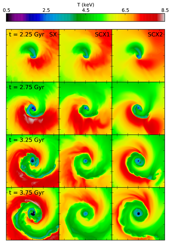
Figure 13.— Slices through the center of the domain in the $x-y$ plane of the temperature for the sloshing simulations with cooling for the epoch $t$ = 2.25, 2.75, 3.25, and 3.75 Gyr. Each panel is 500 kpc on a side. The colorscale is temperature in keV. Major tick marks indicate 100 kpc distances.

We now include radiative cooling in our simulations. The runs with radiative cooling SCX1 and SCX2 correspond to the non-cooling runs SC1 and SC2. The cooling is “turned on” at the same moment as the anisotropic conduction, at the epoch $t$ = 2 Gyr. As control cases to isolate the effects of sloshing and conduction, we also ran the following simulations. RX is an initially relaxed cluster left in isolation without heat conduction. Due to the absence of any heating mechanism, it experiences a cooling catastrophe in the core within a few hundred Myr. RCX is a similar run with an isolated cluster, except it also includes Spitzer conduction along the field lines. Thermal conduction partially offsets the cooling of the core in this run, but the HBI quickly reorients the magnetic field lines in the core in the azimuthal direction and a cooling catastrophe still occurs. The last run, SX, is identical to simulation S1 (without conduction and with sloshing), but with radiative cooling included.

In ZMJ10, we showed that radiative cooling may be slowed by sloshing itself, due to the mixing of hot gas from the outskirts with the cold gas for the core. However, the inclusion of even weak magnetic fields reduces this mixing and inhibits the consequent heating of the core, depending on the strength of the magnetic field (ZML11). From our results in ZMJ10, we expect that regardless of the strength of the magnetic field, the heat delivered to the core from sloshing alone will not be sufficient to prevent a cooling catastrophe at the innermost regions of the cool core. The left panels of Figure 13 shows slices of temperature through the center of the cluster for selected epochs for the SX simulation. In this run, the core temperature drops below 1 keV within a radius of $r\sim 20$ kpc. Additionally, the core density peaks at high values of $n_{e}\sim 1-5$ cm^-3, in conflict with observations of real clusters. Therefore, the goal of the runs with conduction and cooling is to determine if sloshing with conduction together is able to prevent such a cooling catastrophe.

The center and right panels of Figure 13 shows slices of temperature through the center of the cluster for selected epochs for the sloshing simulations including cooling and conduction. Anisotropic conduction, even in the case where it is most efficient, is unable on its own to suppress the runaway cooling in the very center of the cluster, with central temperatures falling to the temperature floor of our simulation ($T\sim 0.01$ keV), far below the temperatures observed in real clusters. However, the temperature is significantly raised outside the very central region of the cool core, at radii $r\,\hbox{\lower 2.58334pt\hbox{$\sim$}\hbox to0.0pt{\hss\raise 2.58334pt\hbox{$>$}}}\,10$ kpc.

The two leftmost panels of Figure 14 show the evolution of the gas mass with short cooling times within the inner 50 kpc of the cluster center over time. We were only able to run the RX simulation out to an epoch of $t\sim 3.6$ Gyr, as the extremely high densities, low temperatures, and magnetic pressures in this simulation made the simulation too unstable to continue past this point. Finally, we have also included a cooling run SXNoB, identical to simulation SX, but without magnetic fields, to compare the rate of increase of cool gas when the mixing of hot and cool gases is not suppressed by such fields. This the same simulation as in ZMJ10, but the setup (resolution and model for the gravitational potential) is identical to our present work, to enable a direct comparison.

The top panels of Figure 14 show the evolution of the gas mass with short cooling times within the inner 50 kpc of the cluster center over time. We were only able to run the RX simulation out to an epoch of $t\sim 3.6$ Gyr, as the extremely high densities, low temperatures, and magnetic pressures in this simulation made the simulation too unstable to continue past this point. Finally, we have also included a cooling run SXNoB, identical to simulation SX, but without magnetic fields, to compare the rate of increase of cool gas when the mixing of hot and cool gases is not suppressed by such fields. This the same simulation as in ZMJ10, but the setup (resolution and model for the gravitational potential) is identical to our present work, to enable a direct comparison.

Over the course of $\sim$2 Gyr, all of the simulations have a significant increase of the mass of cool gas in their cores. However, both sloshing and conduction reduce the buildup of cool gas. The top-left panel of Figure 14 shows the buildup of gas mass with $t_{\rm cool}<0.1$ Gyr. At the onset of cooling, there is no gas in the core with a cooling time this short. Within $\sim$0.25 Gyr, in the relaxed cluster simulations (RX and RCX), a gas mass of $\sim~{}10^{9}-10^{10}~{}M_{\odot}$ with such cooling time has built up in the core. This is somewhat slowed by conduction in the RCX simulation, and by $t\sim$ 4 Gyr the mass of cool gas is lower than that of the RX simulation by a factor of a few. In the simulations with sloshing (SX and SCX1), the initial buildup of cool gas does not begin until $\sim$0.5 Gyr after the onset of cooling. However, in the SX simulation, the mass of cool gas eventually catches up with that of the RX simulation. Out of all of these simulations, the run with both sloshing and conduction (SCX1) is most effective at suppressing the cooling of the gas for the long term, with nearly an order of magnitude less mass of cool gas in the core than in the RX simulation.

In the case of simulation SXNoB, no gas below $t_{\rm cool}=0.1$ Gyr appears until $\sim$1 Gyr after the onset of cooling. Gas mixing, which is much more efficient in the absence of a magnetic field (or perhaps in the presence of field variations on microscopic scales that would strongly reduce field tension), provides a source of heat to the core gas and prevents the catastrophic cooling of gas until this later stage. However, the mass of cool gas increases quickly after this point and is eventually comparable with that of simulation RCX. This indicates that in the absence of magnetic field tension, strong gas mixing due to sloshing is a comparable source of heat to anisotropic conduction.

The top-right panel of Figure 14 shows the buildup of gas mass with $t_{\rm cool}<1.0$ Gyr. In this case, all simulations already start with the same mass of gas with cooling timescales this short. However, the general trend for each of these simulations is the same as for the case for the gas mass with $t_{\rm cool}<0.1$ Gyr. The runs with conduction (or gas mixing) and sloshing exhibit a slower buildup of cool gas.

The bottom panels of Figure 14 show slices through the $z=0$ plane of the temperature at the epoch $t$ = 3.5 Gyr, with contours marking the surfaces with specific cooling times of 0.1, 0.5, and 1.0 Gyr, for the simulations RX and SCX1. It is clear that the effect of sloshing and conduction together is to reduce the volume of the region with very low cooling times and temperatures. Without conduction and sloshing, a $r\sim 10$ kpc region with $t_{\rm cool}<0.1$ Gyr develops, whereas with both of these effects included, this region is restricted to $r\sim 3$ kpc.

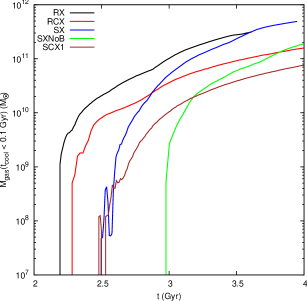
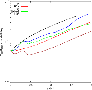
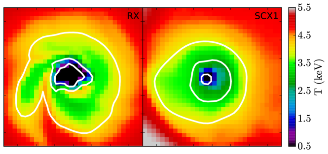
Figure 14.— Top panels: Mass of gas with a cooling time below a given value vs. simulation time for several of the cooling simulations. Left panel: Mass of gas with $t_{\rm cool}<0.1$ Gyr. Right panel: Mass of gas with $t_{\rm cool}<1.0$ Gyr. Bottom panels: Slices through the $z=0$ plane of the temperature in keV for the RX and SCX1 simulations at the epoch $t$ = 3.5 Gyr. White contours mark the surfaces with $t_{\rm cool}$ = 1.0, 0.5, and 0.1 Gyr. Each panel is 75 kpc on a side. Tick marks indicate 10 kpc distances.

Overall, this result indicates that sloshing, even with anisotropic thermal conduction, is not enough to completely stabilize a cool core against a cooling catastrophe, and that for the central regions of clusters, AGN feedback or other mechanisms are necessary to regulate the temperature of the core. However, sloshing and conduction are able to suppress or significantly delay catastrophic cooling in the cluster cooling cores ($r\sim 50-100$ kpc) outside the very central regions of radii $r\,\hbox{\lower 2.58334pt\hbox{$\sim$}\hbox to0.0pt{\hss\raise 2.58334pt\hbox{$<$}}}\,3$ kpc.

4. Discussion and Conclusions

Gas sloshing, a prevalent phenomenon in relaxed galaxy clusters, is evidenced by the nearly ubiquitous presence of spiral-shaped cold fronts in cluster cool cores. The temperature jumps across these fronts imply that either thermal conduction is intrinsically weak in galaxy clusters or the magnetic field is oriented parallel to the front surfaces, restricting conduction across the fronts. Most previous works have assumed the latter, and simulations have confirmed that such magnetic layers form around cold fronts in clusters.

Sloshing may also have an important role in determining the thermal evolution of the cluster core. It brings the cold gas of the core into contact with hot gas, possibly facilitating a transfer of heat between these phases, either via mixing of the hot and cold gas or by heat conduction. This raises the possibility that sloshing may be partially responsible for preventing a “cooling catastrophe” in the cores of galaxy clusters. However, the ICM is magnetized, which, as we showed in ZML11, partially suppresses mixing.

To determine whether anisotropic heat conduction in the presence of magnetic fields has any effect on sloshing cold fronts and the thermal state of the cool cores, we have performed MHD simulations with various configurations of the magnetic field and the conduction coefficients. We determine that, in spite of the fact that the cold fronts indeed are mostly draped by a strong parallel magnetic field, they are not completely thermally isolated from hotter gas. The shear amplification and stretching of magnetic field lines occurs only in a thin layer at some of the cold front surfaces, which only prevents heat conduction to the cold gas below the front from the hot gas directly above the front. Heat can still flow around the cold front, along field lines connected to the cold gas from other regions, either from the hot gas at higher radii perpendicular to the sloshing plane or from the hot flows that are brought inside the cool core by sloshing. Thus, while the sharpness of the temperature gradient at the cold front surfaces may be preserved at some locations along the fronts, the cool gas below the fronts can still be heated from other directions. Also, at some points along the cold front surfaces, the sharpness of the temperature gradient is not preserved because a stabilizing parallel magnetic field layer fails to form. Conduction also leads to the reduction of the density jumps and the widening of the cold front interfaces, which can aid in suppressing Kelvin-Helmholtz instabilities. Importantly, for the hot simulated cluster presented in this work, we find that if conduction is unsuppressed along the field lines, the density jumps can be smoothed to such a degree that the cold fronts are no longer apparent in synthetic X-ray observations, in profound disagreement with observed clusters. Due to the strong temperature dependence of Spitzer conduction, we cannot use our model cluster, which is hot ($T_{X}\sim 8$ keV), to draw conclusions about the smearing out of cold fronts due to conduction in cooler clusters. In a future paper, we will attempt more quantitative comparisons with observed cold fronts in other clusters in order to more generally constrain conduction.

We find that a conduction coefficient parallel to the field lines an order of magnitude smaller than the Spitzer value has a nearly insignificant effect on the temperature of the core and the density and temperature jumps at the cold front surfaces, producing cold fronts that are in agreement with observations. On the other hand, adding even a small perpendicular conduction (0.01 of Spitzer), that may, for example, mimic the effect of field line reconnection, has an effect on the core specific entropy similar to the case with unsuppressed Spitzer conduction along the field lines (because the temperature gradients across the field lines are higher), and slightly smoothes out the temperature gradients of the fronts over the course of a few Gyr.

In the absence of radiative cooling, gas mixing and the conduction of heat between the hot and cold phases in the cluster core raises the temperature and the entropy of the core, and if left unchecked, would eliminate the cool core entirely, leaving behind a high-entropy isothermal core. When radiative cooling is taken into account, we find that, even for full Spitzer conduction along the field lines, a cooling catastrophe still occurs in the cluster center, though the effects of conduction and sloshing together can significantly suppress the buildup of cool gas in the core and restrict the cooling catastrophe to a small ($r\,\hbox{\lower 2.58334pt\hbox{$\sim$}\hbox to0.0pt{\hss\raise 2.58334pt\hbox{$<$}}}\,5$ kpc) volume in the very center. The fact that conduction is unable to suppress cooling completely in the cluster center is somewhat inevitable, as for isobaric perturbations the cooling rate increases with lower temperature and the heating rate from conduction decreases (Kunz et al., 2011). AGN feedback or other mechanisms are still necessary to prevent gas from cooling in these central regions. However, our results show that sloshing and conduction together can produce a significant amount of heat to offset some cooling in the cluster core.

We note that we have only considered one merger scenario and one initial $\beta$ for the magnetic field. Though different choices in these parameter spaces are not expected to change our main conclusions, from our previous works we may make reasonable guesses about the effect of changing our initial conditions. Certain merger setups result in more mixing of hot and cold gases than others (ZMJ10), whereas a lower initial $\beta$ results in stronger magnetic field layers at the cold front surfaces and hence more suppression of K-H instabilities (ZML11). Most importantly for our considerations, the strong temperature dependence of Spitzer conduction makes it particularly strong for our $T\sim 8$ keV simulated cluster. In order to use observations of cold fronts in real clusters to put constraints on suppression of conduction, a wider parameter space of initial cluster temperatures and plasma $\beta$ values would need to be explored. Such a study, including a quantitative comparison with a sample of observed cold fronts, will be presented in a future work.

References

- Asai et al. (2004) Asai, N., Fukuda, N., & Matsumoto, R. 2004, ApJ, 606, L105
- Asai et al. (2005) Asai, N., Fukuda, N., & Matsumoto, R. 2005, Advances in Space Research, 36, 636
- Asai et al. (2007) Asai, N., Fukuda, N., & Matsumoto, R. 2007, ApJ, 663, 816
- Ascasibar & Markevitch (2006) Ascasibar, Y., & Markevitch, M. 2006, ApJ, 650, 102
- Balbus (2000) Balbus, S. A. 2000, ApJ, 534, 420
- Balbus (2001) Balbus, S. A. 2001, ApJ, 562, 909
- Balbus (2004) Balbus, S. A. 2004, ApJ, 616, 857
- Binney & Cowie (1981) Binney, J., & Cowie, L. L. 1981, ApJ, 247, 464
- Bogdanović et al. (2009) Bogdanović, T., Reynolds, C. S., Balbus, S. A., & Parrish, I. J. 2009, ApJ, 704, 211
- Braginskii (1965) Braginskii, S. I. 1965, Reviews of Plasma Physics, 1, 205
- Cavagnolo et al. (2009) Cavagnolo, K. W., Donahue, M., Voit, G. M., & Sun, M. 2009, ApJS, 182, 12
- Chandran et al. (1999) Chandran, B. D. G., Cowley, S. C., Ivanushkina, M., & Sydora, R. 1999, ApJ, 525, 638
- Churazov et al. (2003) Churazov, E., Forman, W., Jones, C., Böhringer, H. 2003, ApJ, 590, 225
- Churazov & Inogamov (2004) Churazov, E., & Inogamov, N. 2004, MNRAS, 350, L52
- Colella & Woodward (1984) Colella, P., & Woodward, P. R. 1984, Journal of Computational Physics, 54, 174
- Cowie & McKee (1977) Cowie, L. L., & McKee, C. F. 1977, ApJ, 211, 135
- Dubey et al. (2009) Dubey, A., Antypas, K., Ganapathy, M. K., Reid, L. B., Riley, K. M., Sheeler, D., Siegel, A., Weide, K. Extensible component based architecture for FLASH, a massively parallel, multiphysics simulation code. Parallel Computing 35 (10-11), 512–522.
- Ettori & Fabian (2000) Ettori, S., & Fabian, A. C. 2000, MNRAS, 317, L57
- Evans & Hawley (1988) Evans, C. R., & Hawley, J. F. 1988, ApJ, 332, 659
- Fryxell et al. (2000) Fryxell, B., et al. 2000, ApJS, 131, 273
- Ghizzardi et al. (2010) Ghizzardi, S., Rossetti, M., & Molendi, S. 2010, A&A, 516, A32
- Govoni et al. (2004) Govoni, F., Markevitch, M., Vikhlinin, A., et al. 2004, ApJ, 605, 695
- Guo et al. (2008) Guo, F., Oh, S. P., & Ruszkowski, M. 2008, ApJ, 688, 859
- Keshet et al. (2010) Keshet, U., Markevitch, M., Birnboim, Y., & Loeb, A. 2010, ApJ, 719, L74
- Keshet (2011) Keshet, U. 2011, arXiv:1111.2337
- Kunz et al. (2011) Kunz, M. W., Schekochihin, A. A., Cowley, S. C., Binney, J. J., & Sanders, J. S. 2011, MNRAS, 410, 2446
- Lecoanet et al. (2012) Lecoanet, D., Parrish, I. J., & Quataert, E. 2012, arXiv:1202.2117
- Lee & Deane (2009) Lee, D., & Deane, A. E. 2009, Journal of Computational Physics, 228, 952
- Lyutikov (2006) Lyutikov, M. 2006, MNRAS, 373, 73
- Malyshkin & Kulsrud (2001) Malyshkin, L., & Kulsrud, R. 2001, ApJ, 549, 402
- Markevitch et al. (2001) Markevitch, M., Vikhlinin, A., & Mazzotta, P. 2001, ApJ, 562, L153
- Markevitch et al. (2003) Markevitch, M., Vikhlinin, A., & Forman, W. R. 2003, Astronomical Society of the Pacific Conference Series, 301, 37
- Markevitch et al. (2003b) Markevitch, M., Mazzotta, P., Vikhlinin, A., et al. 2003, ApJ, 586, L19
- Markevitch & Vikhlinin (2007) Markevitch, M., & Vikhlinin, A. 2007, Phys. Rep., 443, 1
- Mazzotta et al. (2001) Mazzotta, P., Markevitch, M., Vikhlinin, A., Forman, W. R., David, L. P., & VanSpeybroeck, L. 2001, ApJ, 555, 205
- Mewe, Kaastra, & Liedahl (1995) Mewe, R., Kaastra, J. S., & Liedahl, D. A. 1995, Legacy, 6, 16
- Narayan & Medvedev (2001) Narayan, R., & Medvedev, M. V. 2001, ApJ, 562, L129
- O’Hara et al. (2004) O’Hara, T. B., Mohr, J. J., & Guerrero, M. A. 2004, ApJ, 604, 604
- Parrish & Quataert (2008) Parrish, I. J., & Quataert, E. 2008, ApJ, 677, L9
- Parrish et al. (2008) Parrish, I. J., Stone, J. M., & Lemaster, N. 2008, ApJ, 688, 905
- Parrish et al. (2009) Parrish, I. J., Quataert, E., & Sharma, P. 2009, ApJ, 703, 96
- Parrish et al. (2010) Parrish, I. J., Quataert, E., & Sharma, P. 2010, ApJ, 712, L194
- Parrish et al. (2012) Parrish, I. J., McCourt, M., Quataert, E., & Sharma, P. 2012, MNRAS, 2543
- Peterson & Fabian (2006) Peterson, J. R., & Fabian, A. C. 2006, Phys. Rep., 427, 1
- Quataert (2008) Quataert, E. 2008, ApJ, 673, 758
- Roediger & ZuHone (2011) Roediger, E., & Zuhone, J. A. 2011, MNRAS, 1793
- Ruszkowski & Begelman (2002) Ruszkowski, M., & Begelman, M. C. 2002, ApJ, 581, 223
- Ruszkowski et al. (2007) Ruszkowski, M., Enßlin, T. A., Brüggen, M., Heinz, S., & Pfrommer, C. 2007, MNRAS, 378, 662
- Ruszkowski et al. (2008) Ruszkowski, M., Enßlin, T. A., Brüggen, M., Begelman, M. C., & Churazov, E. 2008, MNRAS, 383, 1359
- Ruszkowski & Oh (2010) Ruszkowski, M., & Oh, S. P. 2010, ApJ, 713, 1332
- Ruszkowski & Oh (2011) Ruszkowski, M., & Oh, S. P. 2011, MNRAS, 414, 1493
- Ruszkowski et al. (2011) Ruszkowski, M., Lee, D., Brüggen, M., Parrish, I., & Oh, S. P. 2011, ApJ, 740, 81
- Sarazin (1986) Sarazin, C. L. 1986, Reviews of Modern Physics, 58, 1
- Schekochihin et al. (2005) Schekochihin, A. A., Cowley, S. C., Kulsrud, R. M., Hammett, G. W., & Sharma, P. 2005, ApJ, 629, 139
- Schekochihin et al. (2008) Schekochihin, A. A., Cowley, S. C., Kulsrud, R. M., Rosin, M. S., & Heinemann, T. 2008, Physical Review Letters, 100, 081301
- Sharma & Hammett (2007) Sharma, P., & Hammett, G. W. 2007, Journal of Computational Physics, 227, 123
- Spitzer (1962) Spitzer, L. 1962, Physics of Fully Ionized Gases, New York: Interscience (2nd edition), 1962
- Turk et al. (2011) Turk, M. J., Smith, B. D., Oishi, J. S., Skory, S., Skillman, S. W., Abel, T., & Norman, M. L. 2011, ApJS, 192, 9
- Vikhlinin et al. (2001) Vikhlinin, A., Markevitch, M., & Murray, S. S. 2001, ApJ, 549, L47
- Vikhlinin & Markevitch (2002) Vikhlinin, A. A., & Markevitch, M. L. 2002, Astronomy Letters, 28, 495
- Xiang et al. (2007) Xiang, F., Churazov, E., Dolag, K., Springel, V., & Vikhlinin, A. 2007, MNRAS, 379, 1325
- Zakamska & Narayan (2003) Zakamska, N. L., & Narayan, R. 2003, ApJ, 582, 162
- ZuHone et al. (2010) ZuHone, J. A., Markevitch, M., & Johnson, R. E. 2010, ApJ, 717, 908 (ZMJ10)
- ZuHone et al. (2011) ZuHone, J. A., Markevitch, M., & Lee, D. 2011, ApJ, 743, 16