Investigating the effects of smoothness of interfaces
on stability of probing nano-scale thin films
by neutron reflectometry

Abstract

Most of the reflectometry methods which are used for determining the phase of complex reflection coefficient such as reference method and Variation of Surroundings medium are based on solving the Schrödinger equation using a discontinuous and step-like scattering optical potential. However, during the deposition process for making a real sample the two adjacent layers are mixed together and the interface would not be discontinuous and sharp. The smearing of adjacent layers at the interface (smoothness of interface), would affect the reflectivity, phase of reflection coefficient and reconstruction of the scattering length density (SLD) of the sample. In this paper, we have investigated the stability of reference method in the presence of smooth interfaces. The smoothness of interfaces is considered by using a continuous function scattering potential. We have also proposed a method to achieve the most reliable output result while retrieving the SLD of the sample.

Key words: neutron reflectometry, thin films, smooth potential, reference method

PACS: 68.35.-p, 63.22.Np

Abstract

Бiльшiсть методiв рефлектометрiї, що використовуються для визначення фази комплексного коефiцiєнту вiдбивання такi як еталонний метод i змiна прилеглого середовища грунтуються на розв’язку рiвняння Шредiнгера з використанням розривного i сходинкоподiбного оптичного потенцiалу розсiювання. Проте, пiд час процесу напорошування для пiдготовки реального зразка два сусiднi шари змiшуються i мiжфазова границя може не бути розривною i чiткою. Розмивання сусiднiх шарiв при мiжфазовiй границi (гладкiсть iнтерфейсу), може мати вплив на вiдбивання, фазу коефiцiєнта вiдбивання i перебудову густини довжини розсiювання зразка. В цiй статтi ми дослiдили стiйкiсть еталонного методу у присутностi гладких мiжфазових границь. Гладкiсть мiжфазових границь розглядається, використовуючи неперервну функцiю потенцiалу розсiювання. Ми також запропонували метод для отримання найбiльш надiйного результату, який вiдновлює густину довжини розсiювання зразка.

Ключовi слова: нейтронна рефлектометрiя, тонкi плiвки, гладкий потенцiал, еталонний метод

1 Introduction

In the past decades, neutron reflectometry has been developed as an atomic-scale probe with applications to the study of surface structure ranging from liquid surfaces to the solid thin films. The type and thickness of the nanostructure materials can be determined from measuring the number of neutrons, reflected elastically and specularly from the unknown sample [1, 2, 3].

Neutron reflectometry problems are generally divided into two groups; ‘‘Direct problems’’ and ‘‘Inverse problems’’. The goal of the direct problems is to solve the Schrödinger equation for a distinct sample so that the neutron wave function is determined; On the other hand, the application of inverse problems is to extract the information of the interacting potential by using the complex reflection coefficient [1].

Measuring the intensity of reflected neutrons in terms of the perpendicular component of neutron wave vector to the surface, $q$, provides us with useful information about the scattering length density of the sample along its depth. As with any scattering technique in which only the intensities are measured, the loss of the phase of reflection would result in unresolvable ambiguities on retrieving the SLD from measurement. Without the knowledge of the phase of reflection, more than one SLD can be found for the same reflectivity data. By knowing the phase of the reflection, a unique result would be obtained for the depth profile of the unknown sample [4, 5].

In the recent years, several methods have been worked out for determining the complex reflection coefficient such as: Dwell time method, variation of surroundings medium and the reference layer method which seems to be the most practical [1].

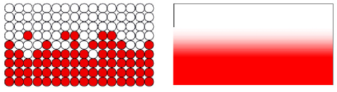
(a)             (b)

Figure 1: Smearing of the SLD of two adjacent layers at the interface. The SLD of layer have been mixed together during the deposition process. (a) Smearing of layers in atomic scale. (b) Continuous variation of SLD at the interface in one dimension.

All of these methods are worked out for an ideal sample in which the interface of two adjacent layers is discontinuous and sharp. In this case, the reflection coefficient is determined by the solution of one dimensional Schrödinger equation for a step-like optical potential. However, as we know from a real sample, there is some smearing at the boundaries. This generally happens during the deposition of a top layer which is miscible with the bottom material (figure 1). This process is strongly temperature dependent. In this case, the interface is defined as a thin layer across which, the SLD of the sample varies smoothly around the mean position of the interface [6].

In most of the simulation methods, the reflectivity measurement and phase determination process is performed for an ideal sample. Considering a continuous and smooth varying optical potential at the interface, it would affect the retrieved reflection coefficient. In the present work, we have studied the effects of potential smoothness on retrieving the depth profile of the sample and the phase of the reflection by considering a continuous potential at boundaries, using reference layers method. As retrieving the SLD from the real and imaginary part of the reflection coefficient is very sensitive, we are going to investigate the way one can find the characteristics of an unknown sample in the presence of the smoothness effects.

2 Theory and method

Interaction of neutron with nuclei is demonstrated by the neutron optical potential $v(z)$, which is a function of the scattering length density of the sample, $v(z)=2\pi\hbar^{2}\rho(z)/4\pi$ where $\rho(z)$ is the scattering length density (SLD) profile as a function of the coordinate $z$; normal to the sample surface [2, 7]. As the thickness of the sample is of the order of nanometer, multiple scattering is neglected in neutron specular reflectometry and the neutron specular reflection is accurately described by a one-dimensional Schrödinger wave equation

$$\left\{\partial_{z}^{2}+\left[q_{0}^{2}-4\pi\rho(z)\right]\right\}\psi(q,z)=0,$$ (1)

where $\psi(q,z)$ is the neutron wave function and $q_{0}$ is the $z$-component of the incident neutron wave vector in vacuum.

Specular reflection is rigorously invertible, however, if both the modulus and the phase of the complex reflection coefficient, $r(q_{0})$, were known, a unique result for scattering length density, $\rho(z)$ would be determined [5].

An exact relation for the reflection coefficient $r(q_{0})$ can be derived from the transfer matrix which is a $2\times 2$ matrix with the elements $A(q_{0}),B(q_{0}),C(q_{0})$, and $D(q_{0})$ which are determined by solving the equation (1), for a film with SLD $\rho(z)$ [3, 7].

Correspondingly, for a sample with arbitrary surroundings, the solution of equation (1) in terms of the transfer matrix elements is represented by:

$$\begin{pmatrix}1\\ \mathrm{i}h\\ \end{pmatrix}t\mathrm{e}^{\mathrm{i}hqL}=\begin{pmatrix}A&B\\ C&D\\ \end{pmatrix}\begin{pmatrix}1+r\\ \mathrm{i}f(1-r)\\ \end{pmatrix},$$ (2)

where $t(q)$ is the transmission coefficient and $f$ and $h$ are the refractive index of the fronting and backing medium having SLD values of $\rho_{f}$ and $\rho_{h}$ respectively. For non-vacuum surroundings, $n=\Big{(}1-4\pi\frac{\rho_{n}}{q_{0}^{2}}\Big{)}^{1/2}$ where $n$ stands for $f$ and $h$. Correspondingly, for vacuum fronting or backing $n(q)=f=h=1$ [1].

The transfer matrix has a unit determinant and is unimodular;

$$A(q_{0})D(q_{0})-B(q_{0})C(q_{0})=1.$$ (3)

As the other property of the transfer matrix, reversing the potential, $\rho(z)\longrightarrow\rho(L-z)$, would cause the interchange of the diagonal elements $A$ and $D$ without having any effect on the off-diagonal elements, $B$ and $C$ [1].

By solving the equation (1) for the reflection coefficient, $r(q)$, we have:

$$r=\frac{\left(f^{2}h^{2}B^{2}+f^{2}D^{2}\right)-\left(h^{2}A^{2}+C^{2}\right)-2\mathrm{i}\left(fh^{2}AB+fCD\right)}{\left(f^{2}h^{2}B^{2}+f^{2}D^{2}\right)+\left(h^{2}A^{2}+C^{2}\right)+2fh}\,.$$ (4)

The reflectivity $R(q)=|r(q)|^{2}$ can be represented in terms of the transfer matrix elements by introducing a new quantity $\Sigma(q)$:

$$\Sigma(q)=2\frac{1+R^{fh}}{1-R^{fh}}=\left(f^{2}h^{2}B^{2}+f^{2}D^{2}\right)+\left(h^{2}A^{2}+C^{2}\right)$$ (5)

where $R$ is the amplitude of the complex reflection coefficient and the superscript $fh$, denotes a sample with fronting and backing medium with refractive index $f$ and $h$, respectively. By introducing the following new quantities

$$\alpha^{fh}=\left(f^{-1}hA^{2}+f^{-1}h^{-1}C^{2}\right),$$

$$\beta^{fh}=\left(fhB^{2}+fh^{-1}D^{2}\right),$$

$$\gamma^{fh}=hAB+h^{-1}CD.$$ (6)

Equations (4) and (5), are represented as

$$r^{fh}=\frac{\beta^{fh}-\alpha^{fh}-2\mathrm{i}\gamma^{fh}}{\beta^{fh}+\alpha^{fh}+2}\,,$$ (7)

$$\Sigma(q)=\beta^{fh}+\alpha^{fh}.$$ (8)

These two equations are the two key relations in reference method. Equation (2) shows that below the critical wave number $q_{\mathrm{c}}=4\pi{\rm Max}\left(\varrho_{f},\varrho_{h}\right)^{1/2}$, the method is not applicable since the information of $r(q)$ is not available. However, the missing data below the $q_{\mathrm{c}}$ could be accurately retrieved by extrapolation [1, 7]. In section 4 we will introduce an algebraic method for determining the missing value below the critical $q$.

2.1 Reference layer method

Here we explain how one can find the complex reflection coefficient of any unknown non-absorptive layer by using some reference layers. Suppose a known layer has been mediated between the fronting medium and the unknown layer. In this case, the transfer matrix of the whole sample (containing the known and unknown layers) can be expressed by the multiplication of the transfer matrix of each one as follows:

$$\begin{pmatrix}A&B\\ C&D\\ \end{pmatrix}=\begin{pmatrix}a&b\\ c&d\\ \end{pmatrix}\begin{pmatrix}w&x\\ y&z\\ \end{pmatrix},$$ (9)

where $(a,\dots,d)$ refer to the matrix elements of the unknown part and $(w,\dots,z)$ present the matrix elements of the known part. Consequently we have

$$\Sigma=\left(h^{2}a^{2}+c^{2}\right)\left(w^{2}+f^{2}x^{2}\right)+\left(h^{2}b^{2}+d^{2}\right)\left(y^{2}+f^{2}z^{2}\right)+2\left(h^{2}ab+cd\right)\left(wy+f^{2}xz\right).$$ (10)

Alternatively, the above formula can be denoted in compact notation in terms of three unknown real-valued parameters as

$$\Sigma(q)=2\frac{1+R^{fh}}{1-R^{fh}}=h^{2}\widetilde{\beta}^{ff}_{\mathrm{K}}\alpha^{hh}_{\mathrm{U}}+f^{2}\widetilde{\alpha}^{ff}_{\mathrm{K}}\beta^{hh}_{\mathrm{U}}+2fh\widetilde{\gamma}^{ff}_{\mathrm{K}}\gamma^{hh}_{\mathrm{U}}\,,$$ (11)

where the subscripts $\mathrm{K}$ and $\mathrm{U}$ refer to the known and unknown parts of the sample and the tilde represents the parameters of the sample with mirror reversed potential $(A\longleftrightarrow D)$. $ff$ and $hh$ denote the same fronting and backing media having the SLD values of $\rho_{f}$ and $\rho_{h}$, respectively.

In order to determine the reflection coefficient, $r(q)$, we consider three measurements of reflectivity for the three known reference layers. Using equation (2) and (11) for three different reference layers $(\rm K_{1},\rm K_{2},\rm K_{3})$, three equations will be obtained. By solving these equations in matrix algebra as shown in equation (12), the parameters $(\alpha^{hh}_{\mathrm{U}},\beta^{hh}_{\mathrm{U}},\gamma^{hh}_{\mathrm{U}})$ are determined which represent the $r^{hh}(q)$ for the unknown film in contact with a uniform identical surroundings in front and back with $\rho_{h}$.

$$\begin{pmatrix}\alpha^{hh}_{\mathrm{U}}\\ \beta^{hh}_{\mathrm{U}}\\ \gamma^{hh}_{\mathrm{U}}\end{pmatrix}={\bf M}\begin{pmatrix}\Sigma_{1}\\ \Sigma_{2}\\ \Sigma_{3}\end{pmatrix},\qquad{\bf M}=\begin{pmatrix}h^{2}\widetilde{\beta}^{ff}_{\mathrm{K}_{1}}&f^{2}\widetilde{\alpha}^{ff}_{\mathrm{K}_{1}}&2fh\widetilde{\gamma}^{ff}_{\mathrm{K}_{1}}\\ h^{2}\widetilde{\beta}^{ff}_{\mathrm{K}_{2}}&f^{2}\widetilde{\alpha}^{ff}_{\mathrm{K}_{2}}&2fh\widetilde{\gamma}^{ff}_{\mathrm{K}_{2}}\\ h^{2}\widetilde{\beta}^{ff}_{\mathrm{K}_{3}}&f^{2}\widetilde{\alpha}^{ff}_{\mathrm{K}_{3}}&2fh\widetilde{\gamma}^{ff}_{\mathrm{K}_{3}}\end{pmatrix}^{-1}.$$ (12)

For $q>q_{\rm c}$ this gives us the reflection coefficient

$$r_{\mathrm{U}}^{hh}=\frac{\beta_{\mathrm{U}}^{hh}-\alpha_{\mathrm{U}}^{hh}-2\mathrm{i}\gamma_{\mathrm{U}}^{hh}}{\beta_{\mathrm{U}}^{hh}+\alpha_{\mathrm{U}}^{hh}+2}\,,$$ (13)

which is equivalent to the reflectivity of a ‘‘free film’’ defined by $\rho_{\mathrm{equiv}}(z)=\rho_{\mathrm{U}}(z)-\rho_{h}$. By inverting $r_{\mathrm{U}}^{hh}$ and shifting by a known constant value, the SLD of the free film can be retrieved [1, 8].

2.2 Determining the phase below the critical wave number

There are several ways for retrieving the missing data below the critical wave number such as extrapolation or using polarized neutron and a magnetic substrate. Here we introduce an algebraic method to retrieve the data below $q_{\rm c}$.

The transfer matrix for a layer having constant SLD in terms of wave number is represented by:

$${\bf T}=\begin{pmatrix}\cos nq_{0}L&\frac{1}{n}\sin nq_{0}L\\ -n\sin nq_{0}L&\cos nq_{0}L\end{pmatrix},$$ (14)

where $n=\sqrt{1-4\pi\varrho/q_{0}^{2}}$, $L$ is the thickness and $\varrho$ is the SLD of the sample.

Introducing several new parameters, $\varrho_{\rm eq}=\varrho-\varrho_{h}$, $q_{\rm eq}=\sqrt{q_{0}^{2}-4\pi\varrho_{h}}$ and $n_{\rm eq}=\sqrt{1-4\pi\varrho_{\rm eq}/q_{\rm eq}^{2}}$, for ${\bf T}$ we have

$${\bf T}=\begin{pmatrix}\cos n_{\rm eq}q_{\rm eq}L&\frac{1}{hn_{\rm eq}}\sin n_{\rm eq}q_{\rm eq}L\\ -hn_{\rm eq}\sin n_{\rm eq}q_{\rm eq}L&\cos n_{\rm eq}q_{\rm eq}L\end{pmatrix}.$$ (15)

By inserting the elements of transfer matrix in equation (13) and using equation equation (7), we have:

$$r^{hh}(\varrho)\Big{|}_{q_{0}=\sqrt{4\pi\varrho_{h}}}=r^{11}(\varrho-\varrho_{h})\Big{|}_{q_{j}=\sqrt{q_{0}^{2}-4\pi\varrho_{h}}}\,.$$ (16)

Equation (16) shows that knowing $r^{hh}(\varrho)$ for $q_{0}\geqslant\sqrt{4\pi\varrho_{h}}$, the reflection coefficient of a free sample having SLD value of $\varrho_{\rm eq}=\varrho-\varrho_{h}$, $r^{11}(\varrho-\varrho_{h})$, is known for specific wave number $q_{j}=\sqrt{q_{0}^{2}-4\pi\varrho_{h}}$ for $q_{j}\geqslant 0$.

2.3 Smooth variation of interface

As we mentioned in section 2.1, there is some smearing at boundaries in real samples and the SLD varies smoothly and continuously from one layer to another. The smooth variation of SLD at boundaries can be expressed by Error function as follows [9]:

$$\varrho(z)=\varrho_{1}(z)+\frac{\varrho_{2}(z)-\varrho_{1}(z)}{2}\left[1+\mathrm{erf}\left(\frac{z-\Delta}{\sqrt{2}\sigma}\right)\right],$$ (17)

where $\sigma$ is the smoothness factor. In other word, $\sigma$ is the thickness of the smoothly varying area across the interface. $\Delta$ is also the mean position of the interface or the turning point of the Error function. Since the reference layer method is based on discontinuity of the interfacial potential, it is obvious that the effect of smoothness at boundaries would affect the reconstruction procedure. In the next section we have investigated these effects numerically.

3 Numerical example

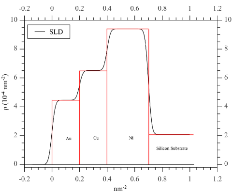
Figure 2: A known reference layer over the Cu-Ni sample with smooth potential at boundaries. The red lines demonstrate the ideal sample with non-smooth boundaries.

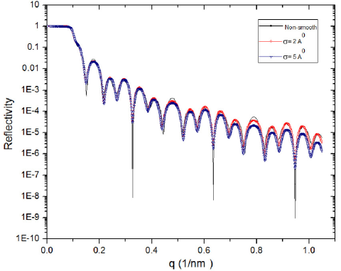
Figure 3: (Color online) Reflectivity from the sample of figure 2 for three cases: $\sigma=0,\ 0.2$ and 0.5 nm.

As a realistic example to study the stability of the reference method by using a smooth potential, we consider a sample with 20 nm thick Copper on 30 nm Nickel having a constant SLD of $6.52\times 10^{-4}$ nm^-2 and $9.4\times 10^{-4}$ nm^-2 as the unknown layer; and three separate reference layers with 20 nm Au, 15 nm Cr and 10 nm Co having a constant SLD value of $4.46,3.03$ and 2.23 ($\times 10^{-4}$ nm^-2), respectively. Figure 2 shows this configuration for the gold layer as reference. Figure 3 also shows the reflectivity of the sample of figure 2 for three difference smoothness factors. The smearing of potential at boundaries is taken into account by using $\sigma=0,\ 0.2$ and 0.5 nm. The effects of smoothness on output results are clear in the figure, particularly at large wave numbers, while the data for small wave numbers truly correspond with none-smooth data.

Reflectivity of the unknown part of the sample with smooth varying SLD at the interface with $\sigma=5$ Å is illustrated in figure 4 (upper curve). Similar to figure 3, the effects of smoothness are more obvious at large wave numbers. However, consideration of smoothness at interface would cause some abrupt noises at certain values of wave numbers such as: $q\simeq 0.3$ and 0.6 nm^-1. The noises also appear for the real and imaginary data of reflection coefficient (figure 5 (a), (b)). These noises are due to the abrupt changes in some of the elements of the ${\bf M}$ matrix, equation (12), in the reference method. The intensity and distribution of these noises along the different ranges of wave numbers are extremely relevant to the smoothness factor, thickness of the reference layers and the range of neutron wave numbers. In order to better understand the origin of these noises, we have plotted the ${\bf M}(3,3)$ element of the ${\bf M}$ matrix in figure 4 (lower curve). The result shows that ${\bf M}(3,3)$ has some noises in $q$ values, exactly as for the reflectivity data. Such severe noises in output results would cause a complete loss of reflection coefficient data in those $q$ values. As we mentioned in section 2, the data of reflection coefficient in the whole range of wave numbers, even bellow the critical wave number, are needed to retrieve the SLD of the sample. Unfortunately, the noises are distributed over different values of wave numbers ranging from small to large $q$’s. This deficiency makes the data useless in retrieving the SLD of the sample. Here we are going to propose a method for removing or reducing these noises.

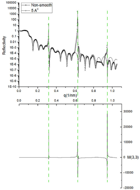
Figure 4: Reflectivity of the unknown sample of figure 2 which is reconstructed by using three reference layers: 20 nm gold, 15 nm Cr and 10 nm Co (Circled curve is for $\sigma=0.5$ nm and solid line is for the ideal sample, $\sigma=0$). ${\bf M}(3,3)$ element of the ${\bf M}$ matrix, equation (12), is plotted for better understanding of the origin of reflectivity noises.

The stability of the method to a great extent depends on the ${\bf M}$ matrix which is a function of the known part of the sample. The best result for the reflection coefficient of the unknown part of the sample comes out of the equation (12) in the case where the behavior of the ${\bf M}$ matrix is smooth. Our investigation shows that not every arbitrary reference layer can lead to a smooth result for the ${\bf M}$ matrix. Since we can control the choice of the reference layers, we can run a simulation to find the best layers for which the ${\bf M}$ matrix behaves smoothly and without noise. By choosing the best reference layer, we can retrieve reliable results for the unknown part of the sample. Those reference layers which are well behaved can be used for experimental implementation of the reflectometry experiments. As we mentioned before, the noise strongly depends on the thickness of the reference layers, and the choice of a proper thickness for the reference films would enhance the accuracy of the output results. In our example, the numerical calculations show that the best result with the smallest noise level would be obtained for 15, 10 and 20 nm thicknesses for Au, Co and Cr, respectively. The purified curves of real and imaginary parts of reflection coefficient in this case are shown in figures 6 (a), (b). As it is clear in the figure, we have much better results with less noise in comparison with figure 5.

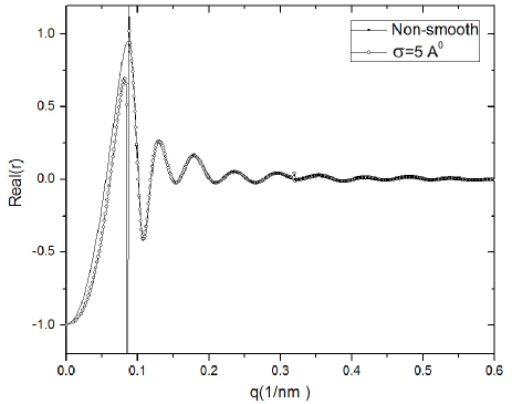
(a)
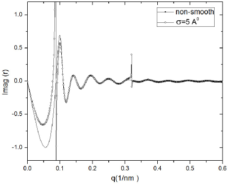
(b)

Figure 5: The reflection coefficient of the unknown part of the sample of figure 2 for two different $\sigma=0$, 5 Å by three reference layers as; 20 nm Au, 15 nm Cr and 10 nm Co. (a) Real and (b), imaginary parts of the reflection coefficient.

Thereupon, the choice of an appropriate thickness for the reference layers would completely remove the noise or displace it to large wave numbers, where it would cause no ambiguity in retrieving the SLD profile of the sample. The rest of the noises can be removed by extrapolation. By using these corrected data as input for some useful codes such as the one which is developed by Sacks [10, 11, 12] based on the Gel’fand-Levitan integral equation [1, 2, 3], the scattering length density of the sample is retrieved. The data of reflection coefficient up to $q=0.6$ are sufficient to retrieve the SLD by Sacks code and we can neglect the data of large wave numbers. Hence, after purification of data, any remaining noise in the range of large wave numbers can be neglected.

The SLD profile corresponding to $r^{hh}(q)$ was retrieved by using the real and imaginary parts of the reflection coefficient at the presence of the smoothness. As it is shown in figure 7, the method of reference layers is stable at the presence of smoothness and the SLD corresponding to $r^{hh}(q)$ is truly reconstructed. The circled curve depicts the retrieved SLD profile of the sample. The retrieved thicknesses corresponds well with the thickness of the sample.

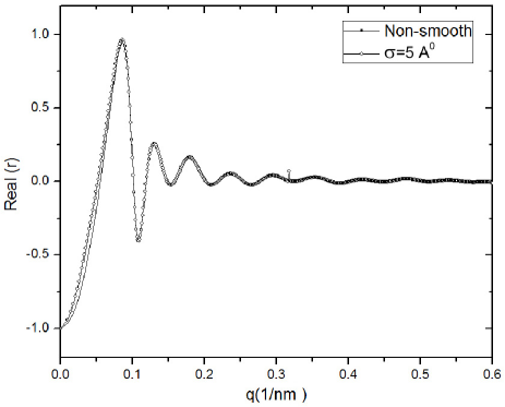
(a)
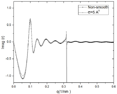
(b)

Figure 6: The reflection coefficient of the unknown part of the sample of figure 2 for $\sigma=0$, 5 Å. The three reference layers are: 15 nm Au, 20 nm Cr and 10 nm Co. Due to the proper selection of reference layers, the noise is removed in comparison with the result of figure 4. (a) Real and (b), imaginary parts of the reflection coefficient.

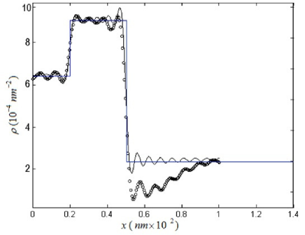
Figure 7: The reconstructed SLD of the unknown sample shown in figure 2, surrounded by identical medium on both sides ($\varrho_{hh}$), obtained by inversion of the extracted values of the reflection coefficient in the momentum range $0\leqslant q\leqslant 0.6$ nm^-1. The non-smooth profile is shown by thin solid line. The circled curve represents the SLD of the sample in the presence of smoothness.

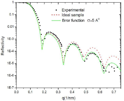
Figure 8: (Color online) Experimental reflectivity curve in contrast to the simulated reflectivity at the presence of smoothness of boundaries and the ideal sample. The green solid line demonstrates the reflectivity at the presence of smoothness and better corresponds with the experimental curve.

Consideration of smoothness of interfaces makes the output results more corresponding to experimental data. In order to verify the efficiency of the method, the reflectivity curves were plotted in figure 8 for a sample from [9], Al₂O₃(6.7 nm)/FeCo(20 nm)/GaAS, for either of smooth (green solid line) and non-smooth boundaries (red dashed line), in contrast to the experimental reflectivity curve. As it is shown in the figure, the reflectivity curve in the presence of smoothness of interfaces better corresponds with the experimental reflectivity curve while the simulated reflectivity for an ideal sample does not absolutely correspond with the experimental curve, particularly at large wave numbers. The results verify that consideration of the smoothness of interfaces is of highest importance.

4 Conclusion

In most of the simulation methods of neutron reflectometry, the SLD of adjacent layers is supposed to be discontinuous and sharp. Since in real samples there is observed some smearing at boundaries, consideration of smoothness would effect the output results and the retrieved data.

In this paper by considering a certain type of Error function which denotes the smooth variation of SLD across the interface and implementing it into the reference method, the effects of smoothness on determining the phase and retrieving the SLD profile of the sample were investigated. Due to consideration of smoothness of interfaces, several abrupt noises existed in the output, such as reflectivity, real and imaginary parts of reflection amplitude. It was shown that these noises are due to the abrupt change in the elements of ${\bf M}$ matrix of equation (12). We proposed to choose a proper thicknesses for the reference layers, which would completely remove the noise or shifted it to the large wave numbers $(q>0.6)$, where the data of reflectivity are not needed in order to retrieve the SLD and we can easily neglect them. Consequently, the SLD of the sample was retrieved by using the purified data of the reflection coefficient.

In order to make sure that the method is highly reliable, we also compared the simulated reflectivity with the experimental curve for a sample. Astoundingly, the results show that consideration of smooth variation of SLD at the interface would make the measured reflectivity to better correspond with the experimental data. The results also certify that the reference method is stable in the presence of smooth interfaces.

Ukrainian 0

Дослiдження впливу гладкостi мiжфазових границь
на стiйкiсть зондуючих наномасштабних тонких плiвок
за допомогою нейтронної рефлектометрiї

С.С. Джаромi, С.Ф. Масудi

             
Фiзичний факультет, Технологiчний унiверситет iм. K.Н. Тусi, а/с 15875-4416, Тегеран, Iран

References

- [1] Majkrzak C.F., Berk N.F., Perez-Salas U.A., Langmuir, 2003, 19, 7796; doi:10.1021/la0341254.
- [2] Zhou X.-L., Chen S.-H., Phys. Rep., 1995, 257, 223; doi:10.1016/0370-1573(94)00110-O.
- [3] Penfold J., Thomas R.K., J. Phys.: Condens. Matter, 1990, 2, 1369; doi:10.1088/0953-8984/2/6/001.
- [4] Kasper J., Leeb H., Lipperheide R., Phys. Rev. Lett., 1998, 80, 2614; doi:10.1103/PhysRevLett.80.2614.
- [5] Masoudi S.F., Pazirandeh A., Physica B, 2005, 356, 21; doi:10.1016/j.physb.2004.10.038.
- [6] Jahromi S.S., Masoudi S.F., Appl. Phys. A, 2010, 99, 255; doi:10.1007/s00339-009-5515-5.
- [7] Majkrzak C.F., Berk N.F., Physica B, 2003, 336, 27; doi:10.1016/S0921-4526(03)00266-7.
- [8] Majkrzak C.F., Berk N.F., Physica B, 1996, 221, 520; doi:10.1016/0921-4526(95)00974-4.
- [9] Fitzsimmons M.R., Majkrzak C.F., Application of polarized neutron reflectometry to studies of artificially structured magnetic materials. In: Modern Techniques for Characterizing Magnetic Materials, edited by Yimei Zhu, Springer, New York, 2005; doi:10.1007/0-387-23395-4_3.
- [10] Klibanov M.V., Sacks P.E., J. Comput. Phys., 1994, 112, 273; doi:10.1006/jcph.1994.1099.
- [11] Chadan K., Sabatier P.C., Inverse Problem in Quantum Scattering Theory, 2nd edn, Springer, New York, 1989.
-
[12]
Aktosun T., Sacks P., Inverse Prob., 1998, 14, 211; doi:10.1088/0266-5611/14/2/001;
Sacks P., Aktosun T., SIAM J. Appl. Math., 2000, 60, 1340; doi:10.1137/S0036139999355588;
Aktosun T., Sacks P., Inverse Prob., 2000, 16, 821; doi:10.1088/0266-5611/16/3/317.
Ukrainian \adddialect\l@ukrainian0 \l@ukrainian