Generalized linear isotherm regularity equation
of state applied to metals

Abstract

A three-parameter equation of state (EOS) without physically incorrect oscillations is proposed based on the generalized Lennard-Jones (GLJ) potential and the approach in developing linear isotherm regularity (LIR) EOS of Parsafar and Mason [J. Phys. Chem., 1994, 49, 3049]. The proposed (GLIR) EOS can include the LIR EOS therein as a special case. The three-parameter GLIR, Parsafar and Mason (PM) [Phys. Rev. B, 1994, 49, 3049], Shanker, Singh and Kushwah (SSK) [Physica B, 1997, 229, 419], Parsafar, Spohr and Patey (PSP) [J. Phys. Chem. B, 2009, 113, 11980], and reformulated PM and SSK EOSs are applied to 30 metallic solids within wide pressure ranges. It is shown that the PM, PMR and PSP EOSs for most solids, and the SSK and SSKR EOSs for several solids, have physically incorrect turning points, and pressure becomes negative at high enough pressure. The GLIR EOS is capable not only of overcoming the problem existing in other five EOSs where the pressure becomes negative at high pressure, but also gives results superior to other EOSs.

Key words: three-parameter equation of state, metallic solids, high pressure, physically incorrect oscillation

PACS: 64.30.Ef, 64.10.+h, 05.70.Ce

Abstract

Запропоновано трипараметричне рiвняння стану без фiзично некоректних осциляцiй, що базується на узагальненому потенцiалi Леннарда-Джонса (GLJ) i пiдходi Парсафара i Мейсона [Parsafar G.A., Mason E.A., J. Phys. Chem., 1994, 49, 3049] до виведення рiвняння стану з регулярнiстю лiнiйної iзотерми (LIR). Запропоноване узагальнене рiвняння стану може включати в себе LIR рiвняння стану як частковий випадок. Трипараметрична узагальнена регулярнiсть лiнiйної iзотерми [Parsafar G.A., Mason E.A., Phys. Rev. B, 1994, 49, 3049] (PM), [Shanker J., Singh B., Kushwa S.S., Physica B, 1997, 229, 419] (SSK), [Parsafar G.A., Spohr H.V., Patey G.N., J. Phys. Chem. B, 2009, 113, 11980] (PSP) i переформульованi PM SSK рiвняння стану є застосованi до 30 металiчних твердих тiл у широкiй областi тиску. Показано, що PM, PMR i PSP рiвняння стану для бiльшостi твердих тiл та SSK i SSKR рiвняння стану для декiлькох твердих тiл мають фiзично некоректнi поворотнi точки, i тиск стає негативним при досить високому тиску. Узагальнене рiвняння стану є здатним не тiльки подолати проблему, iснуючу в iнших п’яти рiвняннях стану, де тиск стає негативним при високому тиску, але також дає кращi результати, нiж iншi рiвняння стану.

Ключовi слова: трипараметричне рiвняння стану, металiчнi твердi тiла, високий тиск, фiзично некоректнi осциляцiї

1 Introduction

The equation of state (EOS) describes the relationships of a system among thermodynamic variables such as pressure, temperature and volume, which plays an important role in many fields, such as condensed-matter physics and geophysics. The Murnaghan [1] and Birch [2, 3] EOSs for solids are widely used in geophysics. Since Rose et al. [4] proposed in 1986 that there exists a universal EOS (UEOS) being valid for all types of solids through analyzing the energy band data, a lot of forms of UEOS have been put forward [5, 6, 7, 8, 9, 10, 11, 12, 13, 14, 15, 16]. However, some of them have been applied to the study of thermodynamic properties of liquids [6, 7, 8, 9, 10, 11, 12, 13, 14, 15, 16, 17, 18, 19], while the traditional Tait EOS has also been used as universal equation both for solids [11, 12] and liquids [13, 14, 15, 16, 17, 18, 19].

In 1994, Parsafar and Mason (PM) proposed the following EOS by using a series expansion of internal energy [11]

$$P\left(\frac{V}{V_{0}}\right)^{2}=C_{0}+C_{1}\left(\frac{V_{0}}{V}\right)+C_{2}\left(\frac{V_{0}}{V}\right)^{2}.$$ (1)

Here, $V_{0}$ is the volume at zero pressure. $C_{0}$, $C_{1}$, $C_{2}$ are three coefficients in the PM EOS. In 1997, Shanker, Singh and Kushwah (SSK) proposed the following EOS [12, 13]

$$P=D_{0}+D_{1}\left(\frac{V_{0}}{V}\right)+D_{2}\left(\frac{V_{0}}{V}\right)^{2},$$ (2)

where $D_{0}$, $D_{1}$, $D_{2}$ are three coefficients in the SSK EOS. It can be seen that the SSK EOS can be expressed as volume-analytic and pressure-analytic forms.

In 1994, Parsafar and Mason proposed the following linear isotherm regularity (LIR) EOS for gases and liquids based on the Lennard-Jones (LJ) (12–6) potential [14]

$$\left(Z-1\right)\left(\frac{V}{V_{0}}\right)^{2}=A_{0}+A_{2}\left(\frac{V_{0}}{V}\right)^{2}.$$ (3)

Here, $Z$ is the compressibility factor, which is equal to $PV/RT$. The upper density limit of LIR [14] is less certain but seems to be the freezing line for liquids ($T<T_{\mathrm{c}}$) and at least about twice the Boyle density for supercritical fluids. LIR EOS has been extended to mixtures [15] and to other forms [16, 17, 18] through adopting different potential functions, including the exponential-6 [16], LJ (6–3) [17], LJ (885–4) [18], and LJ (12–6–3) [19] potentials.

Recently, Parsafar, Spohr and Patey (PSP) [19], extended the equation (3) to the following form with three parameters based on an effective near-neighbor pair interaction of an LJ (12–6–3) potential

$$\left(Z-1\right)\left(\frac{V}{V_{0}}\right)^{2}=A_{0}+A_{1}\left(\frac{V_{0}}{V}\right)+A_{2}\left(\frac{V_{0}}{V}\right)^{2}.$$ (4)

The PSP EOS can be equivalently reformulated as truncated Virial form

$$P=\frac{RT}{V}+\frac{Q_{1}}{V^{2}}+\frac{Q_{2}}{V^{3}}+\frac{Q_{3}}{V^{5}}\,.$$ (5)

Parsafar et al. [19] claimed that the PSP EOS (4) can be applied to all fluids and solids, and their application for solids [19] does not reveal any pressure or temperature limitations.

However, we noticed that the PM EOS (1) and the PSP EOS (4), (5) are physically wrong at high pressure conditions for some solids. This is because the coefficients $C_{2}$ in equation (1) and $A_{2}$ in equation (4) should be positive for all solids to ensure a physically correct tendency at high pressure, $P\rightarrow\infty$ as $V\rightarrow 0$. However, the values of $C_{2}$ for most solids studied in this paper are negative; and the values of $A_{2}$ for solids NaCl and CaO studied by Parsafar et al. [19], and for most solids studied in this paper are also negative. This leads to an unphysical tendency, $P\rightarrow-\infty$ as $V\rightarrow 0$.

The incorrect tendency makes the PM [11] and PSP [19] EOSs inapplicable to high pressure conditions. We may preliminarily analyze the reason for the failure of two EOSs as follows. Holzapfel [20] has pointed out that the limitation of an EOS as the volume tends to zero, should be the Tomas–Fermi (TF) model, $P\propto V^{-5/3}$. The repulsion terms in PM [11] and PSP [19] EOSs are, $P\propto V^{-4}$ and $P\propto V^{-5}$, respectively. Their exponent numbers 4 and 5 are far larger than 5/3, and are too hard for solids. In order to fit experimental $P-V$ data at low and middle pressure ranges, the optimized $C_{2}$ and $A_{3}$ should take on negative values.

In this work, we propose generalized LIR (GLIR) EOS based on a near-neighbor pair potential of the extended Lennard-Jones ($m_{1}$,$n_{1}$) type. The GLIR contains three parameters and can overcome the defect appearing in the PM EOS (1) and PSP EOS (4). In section 2, the three-parameter GLIR EOS is proposed. In section 3, equations (1) and (2) and their modified version, PSP EOS (4) and the GLIR EOS are applied to twenty solids within wide pressure ranges of hundreds GPa and at ambient temperature, the results being analyzed and discussed. In section 4, the conclusion is presented.

2 Analytic equations of state

We adopt the effective pair interaction of an extended Lennard-Jones ($m_{1}$,$n_{1}$) type potential [10, 17, 19, 20]

$$\varepsilon\left(r\right)=\frac{\varepsilon_{0}}{m_{1}-n_{1}}\left[n_{1}\left(\frac{r_{\mathrm{e}}}{r}\right)^{m_{1}}-m_{1}\left(\frac{r_{\mathrm{e}}}{r}\right)^{n_{1}}\right].$$ (6)

It is well known that the effective potentials for metals usually have oscillating tails due to Friedel oscillations of electron density, and the Lennard-Jones (LJ) potentials are not really appropriate for correct reproduction of the energetics of metals. However, many works [10, 11, 12, 13, 14, 15, 16, 17, 18, 19] have shown that the LJ potentials can mimic many properties of metals in some compression ranges. By adopting the nearest neighbor assumption [11], the total configurational energy of a solid is

$$U = \frac{N\delta\varepsilon_{0}}{2\left(m_{1}-n_{1}\right)}\left[n_{1}\left(\frac{r_{\mathrm{e}}}{r}\right)^{m_{1}}-m_{1}\left(\frac{r_{\mathrm{e}}}{r}\right)^{n_{1}}\right]$$ (7)

$$= \frac{N\delta\varepsilon_{0}}{2\left(m_{1}-n_{1}\right)}\left[n_{1}\left(\frac{V_{\mathrm{e}}}{V_{0}}\right)^{m_{1}/3}-m_{1}\left(\frac{V_{\mathrm{e}}}{V_{0}}\right)^{n_{1}/3}\right],$$

where $V=a^{3}/\gamma$, $V_{0}=\left(r_{\mathrm{e}}\right)^{3}/\gamma$, $a$ is the nearest neighbor distance, and $\delta$ is the mean coordination number [10, 19]. Following Parsafar and Mason [8], the internal pressure can be obtained by the derivative of equation (6)

$$P_{\mathrm{int}}=-\frac{\partial U}{\partial V}=\frac{m_{1}n_{1}N\delta\varepsilon_{0}}{6\left(m_{1}-n_{1}\right)}\left[\left(\frac{V_{\mathrm{e}}}{V_{0}}\right)^{m_{1}/3+1}-\left(\frac{V_{\mathrm{e}}}{V_{0}}\right)^{n_{1}/3+1}\right].$$ (8)

Let us substitute the equation (7) into the following internal energy equation

$$P=T\left(\frac{\partial P}{\partial T}\right)_{V}-\left(\frac{\partial U}{\partial V}\right)_{T}\,.$$ (9)

After integration, we derive the equation

$$P=\frac{RT}{V}+A_{1}\left(\frac{V_{0}}{V}\right)^{n_{1}/3+1}+A_{2}\left(\frac{V_{0}}{V}\right)^{m_{1}/3+1}.$$ (10)

Here, $A_{1}$ and $A_{2}$ are functions of temperature.

In order to obtain an extended LIR EOS, we would limit parameters $m_{1}$ and $n_{1}$ to satisfy the relationship, $m_{1}$ = 2 $n_{1}$, and

$$m_{1}/3=2m,\qquad n_{1}/3=m.$$ (11)

Then, equation (7) changes to the following form

$$P=\frac{RT}{V}+A_{1}\left(\frac{V_{0}}{V}\right)^{m+1}+A_{2}\left(\frac{V_{0}}{V}\right)^{2m+1}.$$ (12)

By using definition of compressibility, $Z=PV/RT$, equation (12) can be reformulated following the generalized LIR (GLIR) EOS

$$\left(Z-1\right)\left(\frac{V}{V_{0}}\right)^{m}=B_{0}+B_{1}\left(\frac{V_{0}}{V}\right)^{m},$$ (13)

$$B_{0}=\frac{A_{0}V_{0}}{RT}\,,\qquad B_{1}=\frac{A_{2}V_{0}}{RT}\,.$$ (14)

It can be seen that the LIR EOS in equation (3) can be included in the GLIR EOS (13) as a special case when $m$ = 2. Since $m$ = 1, equation (13) just reduces to the virial EOS. Although the parameter number of PSP EOS (4) is the same as the three-parameter GLIR EOS (13), equation (13) with adjustable parameter $m$ is more flexible and more accurate than equation (4).

Otherwise, we found in our calculations that the PM [11] and SSK [12, 13] EOSs can be reformulated in the following forms:

$$P\left(\frac{V}{V_{0}}\right)^{4} = C_{2}+C_{1}\left(\frac{V}{V_{0}}\right)+C_{0}\left(\frac{V}{V_{0}}\right)^{2},$$ (15)

$$P\left(\frac{V}{V_{0}}\right)^{2} = D_{2}+D_{1}\left(\frac{V}{V_{0}}\right)+D_{0}\left(\frac{V}{V_{0}}\right)^{2}.$$ (16)

We name this form as PMR and SSKR EOSs. Although the PMR EOS and SSKR EOSs are mathematically equivalent to the PM and SSK EOSs, they physically differ from each other. This is because all of equations (1), (2) and equations (15), (16) can be seen as Taylor expansion, but the expansion variable of equations (1), (2) is ($V_{0}$/$V$), and that of equations (15), (16) is ($V$/$V_{0}$). At zero pressure, both values of ($V_{0}$/$V$) and ($V$/$V_{0}$) are equal to 1. At high pressure, the values of ($V$/$V_{0}$) are smaller than 1, the Taylor expansions in equations (15), (16) are fast convergent. However, the values of ($V_{0}$/$V$) are larger than 1 at high pressure, the Taylor expansions in equations (1), (2) are slowly convergent. Thus, the PMR and SSKR EOSs in equations (15), (16) are more accurate than the original PM and SSK EOSs in equations (1), (2).

3 Results and discussion

Now we apply six EOSs to 28 metallic solids, including GLIR (13), PM [11], PMR (15), SSK [12, 13], SSKR (16) and PSP [19] EOSs. All experimental data are taken from Kennedy and Keeler (1972) [21], except for W [22].

Table 1: The experimental data of $V_{0}$ (cm³/mol) and comparison of average relative errors ($\Delta_{\mathrm{p}}$%) of pressure for 30 metallic solids calculated from the GLIR, PM, PMR, SSK, SSKR, and PSP EOSs.

		GLIR	PM	PMR	SSK	SSKR	PSP
	$V_{0}$	$\Delta_{\mathrm{p}}\%$	$\Delta_{\mathrm{p}}\%$	$\Delta_{\mathrm{p}}\%$	$\Delta_{\mathrm{p}}\%$	$\Delta_{\mathrm{p}}\%$	$\Delta_{\mathrm{p}}\%$
Cu	7.115	0.54	0.54	0.50	9.34	4.65	0.43
Mo	9.387	0.80	1.99	1.45	1.08	1.05	1.32
Zn	9.166	0.30	0.55	0.39	9.34	5.46	0.48
Ag	10.27	0.38	0.47	0.41	6.22	4.10	0.45
Pt	9.098	0.70	0.70	0.70	2.15	1.69	0.70
Ti	12.01	0.68	3.38	2.03	2.07	1.07	2.09
Ta	10.80	0.66	1.14	0.86	0.68	0.64	0.89
Au	10.22	0.64	0.64	0.64	2.44	1.80	0.64
Pd	8.896	0.72	0.72	0.72	2.21	1.55	0.72
Zr	14.02	0.62	7.02	4.21	3.70	2.13	3.51
Cr	7.231	0.99	1.00	1.00	1.35	1.20	1.00
Co	6.689	0.65	0.61	0.61	0.60	0.60	0.60
Ni	6.592	0.60	0.61	0.61	1.13	0.98	0.62
Nb	10.83	1.71	1.90	2.00	2.15	2.20	1.76
Cd	13.00	0.24	0.30	0.29	4.08	2.92	0.31
Al	10.00	0.85	0.76	0.76	0.87	0.66	0.49
Th	19.97	0.36	0.95	0.69	0.78	0.53	0.86
V	8.365	0.39	0.70	0.58	0.41	0.39	0.49
In	15.73	0.57	0.76	0.62	3.98	2.91	0.60
Be	4.890	0.43	0.64	0.55	0.61	0.52	0.51
Pb	18.27	0.30	0.31	0.31	2.86	2.06	2.09
Sn	16.32	0.26	0.31	0.29	2.50	1.81	0.29
Mg	14.00	0.33	0.59	0.47	0.27	0.26	0.66
Ca	26.13	0.61	5.67	4.05	2.91	1.69	4.98
Tl	17.23	0.29	0.29	0.29	1.38	1.08	0.28
Na	23.71	0.48	0.94	0.68	0.23	0.21	1.15
K	45.62	0.39	1.30	1.20	0.85	0.46	1.80
Rb	56.08	0.43	1.21	1.15	0.64	0.36	1.75
mean error		0.57	1.29	1.00	2.39	1.61	1.12

In table 1, we list the volume at zero pressure $V_{0}$, average fitting errors of pressure for the 28 solids. It can be seen that the GLIR (13) yields the smallest fitting errors for 20 solids, and for the other 8 solids the errors are also fairly small. The fitting precision for different solids is fairly stable for the GLIR EOS (13), while instable for the other five EOSs. The largest errors among the 28 solids for the six EOSs are 1.71% of Nb, 7.02% of Zr, 4.21% of Zr, 9.34% of Zn, 5.46% of Zn, 4.98% of Ca, respectively. In the last line of the table, we list the total average error for the 28 solids. It can be seen that the GLIR EOS yields the best results with average error 0.57%; the PMR EOS yields second best results with average error 1.00%; the PSP EOS, PM EOS, SSKR EOS, and SSK EOS subsequently give worse results with average errors 1.12%, 1.29%, 1.61% and 2.39%, respectively.

Table 2: Optimized values of coefficients for the GLIR, PM and PMR EOSs determined by fitting experimental compression data. The parameters for the GLIR EOS are dimensionless; and all parameters for PM and PMR EOSs are in GPa.

	GLIR			PM			PMR
	$m$	$B_{0}$	$B_{1}$	$C_{0}$	$C_{1}$	$C_{2}$	$C_{0}$	$C_{1}$	$C_{2}$
Cu	0.906	–449.53	448.57	–153.86	167.29	–13.44	–13.24	166.74	–153.51
Mo	0.592	–1731.45	1732.80	–395.31	458.15	–98.61	–101.51	465.36	–363.72
Zn	1.199	–188.20	187.21	–48.41	34.78	13.53	14.11	33.18	–47.34
Ag	1.197	–368.37	367.35	–81.38	55.72	25.60	26.14	54.37	–80.54
Pt	1.031	–1000.33	999.46	–272.52	263.83	8.69	9.54	261.87	–271.40
Ti	0.416	–1185.34	1184.03	–126.25	164.13	–37.40	–40.20	171.78	–131.30
Ta	0.527	–1655.67	1654.63	–218.00	369.91	–88.75	–90.88	375.05	–284.06
Au	1.004	–762.52	761.51	–184.79	183.79	0.70	1.52	181.85	–183.36
Pd	1.031	–683.16	682.19	–188.56	181.27	7.29	7.11	181.68	188.80
Zr	0.197	–2763.5	2762.6	–122.61	166.63	–43.34	–48.00	179.09	–130.68
Cr	0.924	–609.57	608.36	–209.26	226.66	–17.46	–17.58	226.93	–209.41
Co	0.729	–733.72	732.70	–257.16	318.67	–61.49	–61.29	318.20	–256.89
Ni	0.893	–565.39	564.35	–211.11	234.21	–23.09	–22.88	233.72	–210.83
Nb	0.582	–1282.5	1281.3	–250.03	331.05	–81.09	–82.18	333.60	–251.51
Cd	1.223	–216.51	215.61	–36.99	23.21	13.76	13.84	23.00	–36.86
Al	0.719	–452.88	451.48	–106.33	132.17	–26.01	–25.01	129.71	–104.84
Th	0.613	–701.54	700.18	–65.47	81.33	–15.71	–16.41	83.24	–66.73
V	0.569	–939.67	938.80	–223.73	293.70	–69.84	–70.98	296.38	–225.29
In	1.058	–240.83	239.89	–38.61	36.62	1.930	2.430	35.31	–37.75
Be	0.477	–500.16	499.19	–177.73	239.41	–61.58	–62.52	241.66	–179.05
Pb	1.022	–323.72	322.61	–43.61	42.49	1.090	1.240	42.12	–44.37
Sn	1.118	–256.62	255.80	–37.87	32.02	5.850	5.970	31.72	–37.69
Mg	0.592	–338.70	337.60	–44.32	55.83	–11.41	–11.81	56.91	–45.03
Ca	0.076	–2812.2	2810.9	–20.35	27.60	–6.810	–8.040	31.34	–23.05
Tl	1.154	–216.85	215.66	–28.85	21.85	6.990	7.160	21.43	–28.60
Na	0.540	–112.14	111.09	–6.740	8.370	–1.540	–1.660	8.740	–7.030
K	0.419	–147.58	146.11	–2.900	3.670	–0.670	–0.750	3.980	–3.160
Rb	0.457	–115.00	113.29	–1.780	2.230	–0.360	2.440	–1.970	1.210

In tables 2 and 3, we list the fitted parameters for the six EOSs, table 2 shows that the values of $m$ in the GLIR EOS (13) are smaller than 1 for 19 solids, and slightly larger than 1 for 10 solids. This implies that the interactions in the metals are far softer than the LJ (12–6) potential, and are approximately approaching the LJ (6–3) potential for the 10 solids, and even softer than the LJ (6–3) potential for other 20 solids. The table also shows that the parameter $B_{1}$ in the GLIR EOS (13) always takes on positive values, and this ensures a correct tendency as the volume tends to infinity.

However, the values of $C_{2}$ in the PM and PMR EOSs are negative for 18 and 25 solids, respectively. The values of $D_{2}$ in the SSKR EOS, $A_{2}$ in the PSP EOS are also negative for 2 and 18 solids, respectively. For these solids, the corresponding EOSs may exhibit a physically incorrect tendency as the volume tends to infinity. To compare, the GLIR EOS (13) is not only the most precise one, but also is a unique EOS that does not exhibit a physically incorrect tendency among the six EOSs studied in this work. In figures 1, 2 and 3, we plot the experimental compression data and the curves calculated using the GLIR, PMR, SSKR and PSP for 10 solids, including Cu, Mo, Ag, Ti, Ta, Zr, Ni, Nb, Th and Be. These figures show that the calculated compression curves from the GLIR and SSKR EOSs are correct at high pressure for the 10 solids, although for Zr, the parameter $D_{2}$ in the SSKR EOS takes on a negative value. But the PMR EOS yields incorrect compression curves at high pressure for 7 of 10 solids, except for the solid Cu, Ag, and Ni. And the turn point is in the range $V$/$V_{0}\approx$ ($0.3\div 0.5$) for the 7 solids. Moreover, the PSP EOS also yields incorrect compression curves at high pressure for 9 of 10 solids, except for the solid Ag. And the turn point is about $V$/$V_{0}$ $\approx$ 0.3 for solids Cu and Ni; about $V$/$V_{0}\approx$ 0.5 for other 7 solids.

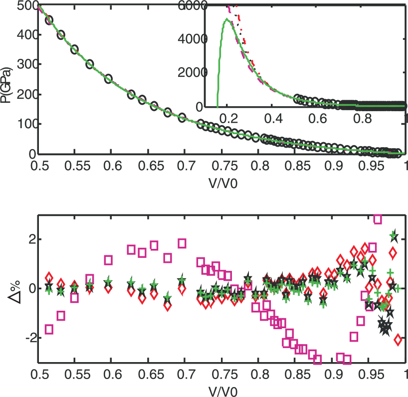
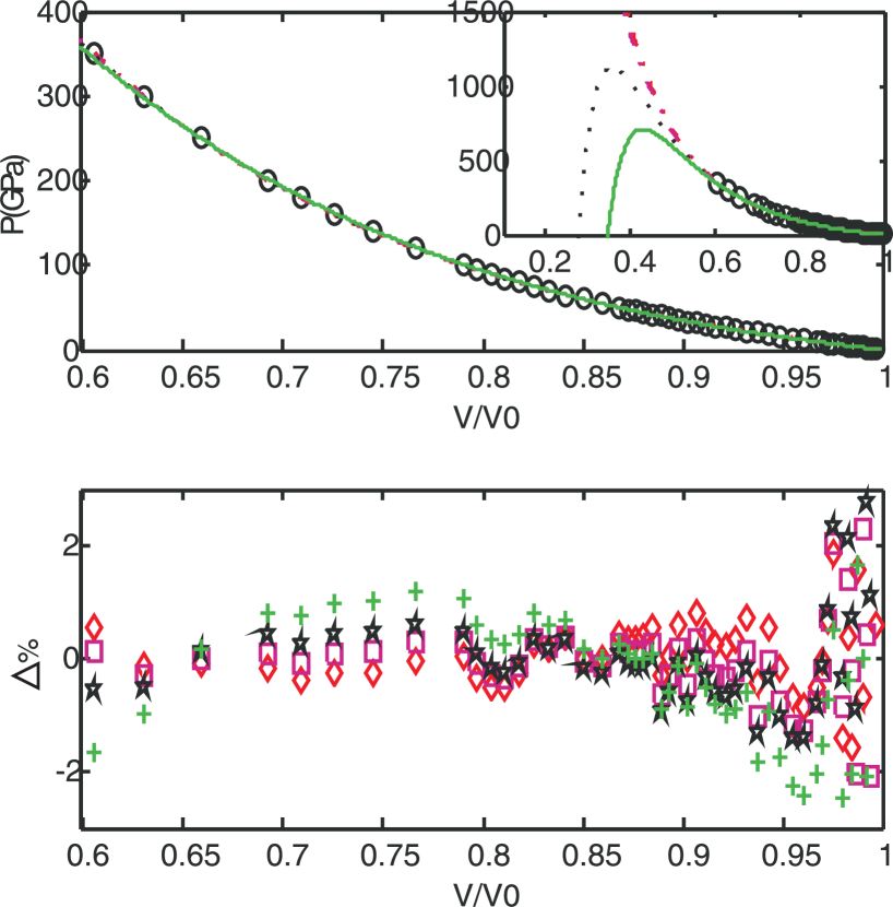
(a)

(b)

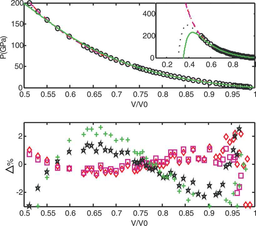
(c)

(d)

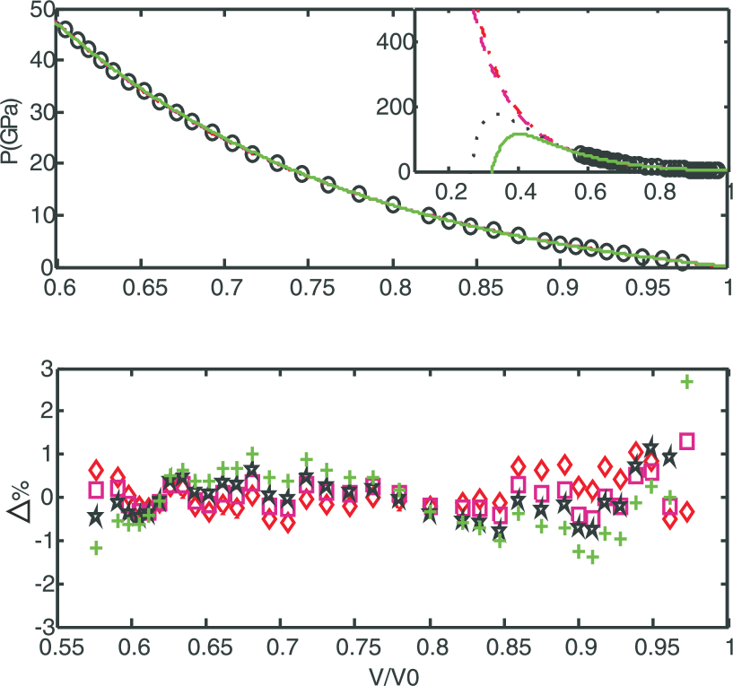
(e)

(f)

Figure 1: (Color online) Comparison of compression curves of Cu (a), Mo (b), Ag (c), Ti (d), Mg (e), and Zr (f) calculated by using different equations with experimental data ($\circ$): solid line, PSP EOS; dashed line, SSKR EOS; dot line, PMR EOS; dot-dashed line, GLIR EOS. And comparison of percentage error of pressure calculated using different equations: $+$, PSP EOS; $\square$, SSKR EOS; $\star$, PMR EOS; $\Diamond$, GLIR EOS.

Table 3: Optimized values of coefficients for the SSK, SSKR and PSP EOSs determined by fitting experimental compression data. The parameters for the PSP EOS are dimensionless; and all parameters for SSK and SSKR EOSs are in GPa.

	SSK			SSKR			PSP
	$D_{0}$	$D_{1}$	$D_{2}$	$D_{0}$	$D_{1}$	$D_{2}$	$A_{0}$	$A_{1}$	$A_{2}$
Cu	293.73	–686.40	394.71	381.53	–650.37	269.96	427.41	–419.20	–9.020
Mo	156.70	–578.16	421.54	421.11	–577.10	156.06	1316.8	–1209.8	–107.85
Zn	260.70	–528.62	271.29	256.94	–489.17	234.34	192.99	–206.99	12.750
Ag	326.55	–720.31	395.34	382.78	–688.72	307.02	359.42	–389.56	28.99
Pt	466.76	–1193.8	727.49	720.07	–1176.7	456.98	996.17	–1008.9	11.81
Ti	8.260	–121.04	112.44	114.63	–127.03	12.22	585.21	–536.06	–49.24
Ta	72.99	–344.84	271.82	272.46	–346.38	73.90	1179.1	–1066.7	–113.03
Au	325.64	–816.00	490.93	484.10	–799.81	316.14	761.26	–763.39	1.120
Pd	344.40	–865.63	521.72	513.51	–846.47	333.32	682.39	–690.84	7.450
Zr	–40.14	–22.08	61.86	64.60	–29.40	–35.39	690.45	–617.45	–73.00
Cr	259.25	–700.19	441.11	437.08	–609.92	253.56	605.12	–591.28	–15.00
Co	161.67	–516.19	354.61	354.11	–515.05	161.00	663.78	–618.34	–46.25
Ni	241.20	–661.39	420.41	417.51	–654.68	237.36	553.90	–537.02	–17.83
Nb	70.990	–313.58	242.46	241.83	–312.12	70.140	1029.9	–931.42	–99.57
Cd	175.83	–376.06	201.58	195.08	–359.21	165.11	211.34	–231.68	19.28
Al	64.27	–207.75	143.33	144.62	–210.93	66.190	39.50	–370.24	–26.01
Th	39.87	–129.44	89.70	89.03	–127.60	38.66	500.66	–467.25	–33.83
V	72.94	–302.04	229.17	228.67	–300.87	72.25	733.25	–663.29	–70.70
In	109.23	–241.91	133.57	129.82	–231.91	102.73	244.77	–249.76	3.890
Be	26.94	–175.10	148.11	148.97	–177.14	28.14	338.68	–303.43	–36.13
Pb	103.88	–239.29	136.04	132.39	–229.89	97.94	276.25	–287.00	11.52
Sn	110.10	–251.61	142.07	138.48	–242.59	104.52	256.41	–268.25	10.89
Mg	21.76	–77.32	55.60	55.56	–77.22	21.69	238.92	–222.07	–17.46
Ca	–14.73	6.430	8.020	8.840	3.940	–12.93	220.27	–198.94	–20.39
Tl	85.87	–200.18	114.59	112.74	–195.66	83.15	210.86	–225.44	13.47
Na	3.410	–12.71	9.300	9.330	–12.81	3.480	61.28	–58.10	–3.550
K	0.170	–3.950	3.700	3.810	–4.330	0.490	48.05	–44.26	–2.410
Rb	0.530	–3.450	2.850	2.910	–3.680	0.750	35.90	–32.56	–1.400

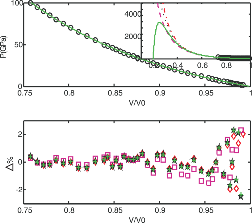
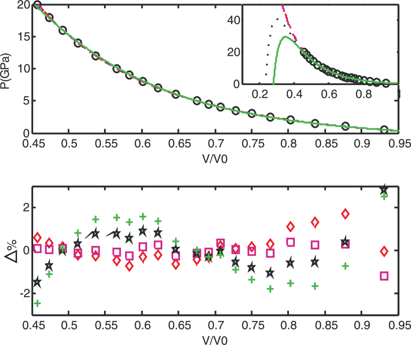
(a)

(b)

Figure 2: (Color online) Comparison of compression curves of Ni (a) and Na (b) calculated by using different equations with experimental data ($\circ$): solid line, PSP EOS; dashed line, SSKR EOS; dot line, PMR EOS; dot-dashed line, GLIR EOS. And comparison of percentage error of pressure calculated using different equations: $+$, PSP EOS; $\square$, SSKR EOS; $\star$, PMR EOS; $\Diamond$, GLIR EOS.

In these figures, we also plot the variation of relative errors of pressure with compression ratio $V$/$V_{0}$. It can be seen from these figures that, for solids Cu and Ag, the oscillations of relative errors from the SSKR EOS are the most prominent, and are the same from other three EOSs; for solids Ti and Zr, the oscillations of relative errors from the PSP EOS and PMR EOS are more evident than the SSKR and GLIR EOSs; and for other solids, the oscillations from all four EOSs are equivalent with each other. It is notable that the relative errors from the GLIR EOS are most stable and fairly small for all 10 solids and for all compression ratio ranges. These results show that the GLIR EOS can be seen as the best one among six EOSs studied in this work.

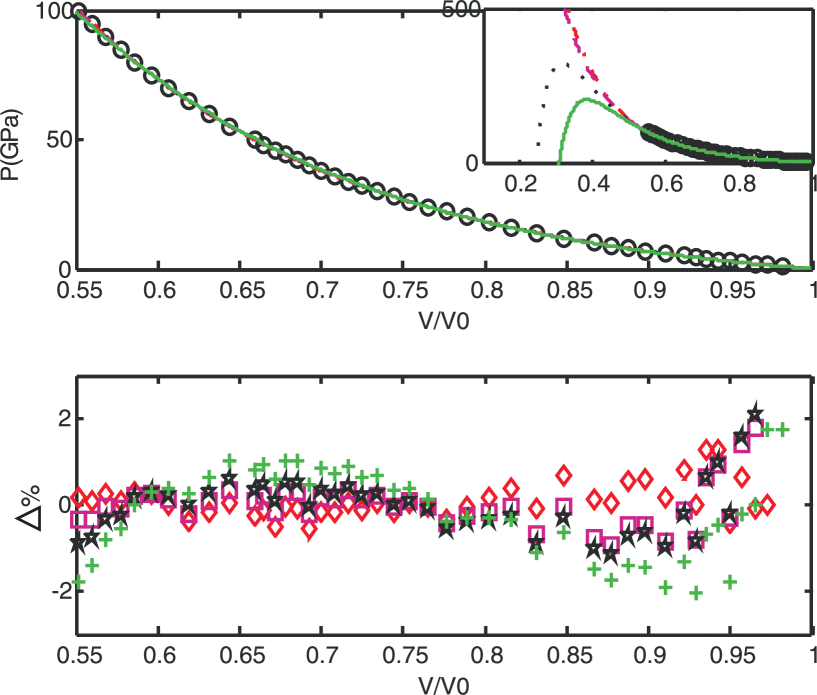
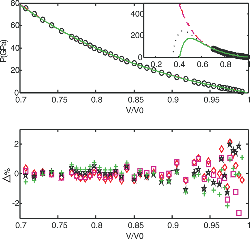
(a)

(b)

Figure 3: (Color online) Comparison of compression curves of Th (a) and Be (b) calculated by using different equations with experimental data ($\circ$): solid line, PSP EOS; dashed line, SSKR EOS; dot line, PMR EOS; dot-dashed line, GLIR EOS. And comparison of percentage error of pressure calculated using different equations: $+$, PSP EOS; $\square$, SSKR EOS; $\star$, PMR EOS; $\Diamond$, GLIR EOS.

4 Conclusion

In conclusion, we develop a three-parameter GLIR based on the GLJ potential and the approach of Parsafar and Mason [14] in developing the LIR EOS. Comparing with other five EOSs popular in literature, the precision of the GLIR EOS developed in this paper is superior to other EOSs. The GLIR EOS is capable of overcoming the problem existing in other EOSs where the pressure becomes negative at high enough pressure conditions.

Ukrainian 0

Узагальнене рiвняння стану, застосовне до металiв

Г. Сан${}^{\textsf{\footnotesize{\mbox{?}}}}$, Дж.Г. Сан${}^{\textsf{\footnotesize{\mbox{?},\penalty 1000\mbox{?}}}}$, В.Дж. Йу${}^{\textsf{\footnotesize{\mbox{?}}}}$, Дж. Танг${}^{\textsf{\footnotesize{\mbox{?}}}}$

             
${}^{\textsf{\footnotesize 1}}$ Кафедра прикладної фiзики, Китайський унiверситет електронiки та технологiй, Ченду 610054, КНР ${}^{\textsf{\footnotesize 2}}$ Лабораторiя фiзики ударної хвилi i детонацiї, Пiвденно-Захiдний iнститут фiзики плинiв,
Мiанян 621900, КНР

References

- [1] Murnaghan F.D., Proc. Natl. Acad. Sci. U.S.A., 1944, 30, 244; doi:10.1073/pnas.30.9.244.
- [2] Birch F., Phys. Rev., 1947, 71, 809; doi:10.1103/PhysRev.71.809.
- [3] Birch F., J. Geophys. Res., 1978, 83, 1257; doi:10.1029/JB083iB03p01257.
- [4] Rose J.H., Smith J.R., Guinea F., Ferrante J., Phys. Rev. B, 1984, 29, 2963; doi:10.1103/PhysRevB.29.2963.
- [5] Vinet P., Smith J.R., Ferrante J., Rose J.H., Phys. Rev. B, 1987, 35, 1945; doi:10.1103/PhysRevB.35.1945.
- [6] Kuchhal P., Kumar R., Dass N., Phys. Rev. B, 1997, 55, 8042; doi:10.1103/PhysRevB.55.8042.
- [7] Schlosser H., Ferrante J., Phys. Rev. B, 1989, 40, 6405; doi:10.1103/PhysRevB.40.6405.
- [8] Baonza V.G., Caceres M., Nunez J., Chem. Phys. Lett., 1994, 228, 137; doi:10.1016/0009-2614(94)00935-X.
- [9] Baonza V.G., Caceres M., Nunez J., J. Phys. Chem., 1994, 98, 4955; doi:10.1021/j100070a001.
- [10] Sun J.X., J. Phys.: Condens. Matter, 2005, 17, L103; doi:10.1088/0953-8984/17/12/L01.
- [11] Parsafar G.A., Mason E.A., Phys. Rev. B, 1994, 49, 3049; doi:10.1103/PhysRevB.49.3049.
- [12] Shanker J., Singh B., Kushwah S.S., Physica B, 1997, 229, 419; doi:10.1016/S0921-4526(96)00528-5.
- [13] Saxena S.K., J. Phys. Chem. Solids, 2004, 65, 1561; doi:10.1016/j.jpcs.2004.02.003.
- [14] Parsafar G., Mason E.A., J. Phys. Chem., 1994, 98, 1962; doi:10.1021/j100058a040.
- [15] Parsafar G., Sohraby N., J. Phys. Chem., 1996, 100, 12644; doi:10.1021/jp960239v.
- [16] Ghatee M.H., Shams-Abadi H., J. Phys. Chem. B, 2001, 105, 702; doi:10.1021/jp001022a.
- [17] Ghatee M.H., Bahadori M., J. Phys. Chem. B, 2001, 105, 11256; doi:10.1021/jp011592q.
- [18] Ghatee M.H., Niroomand-Hosseini F., J. Phys. Chem. B, 2004, 108, 10034; doi:10.1021/jp036977i.
- [19] Parsafar G.A., Spohr H.V., Patey G.N., J. Phys. Chem. B, 2009, 113, 11977; doi:10.1021/jp903519c.
- [20] Holzapfel W.B., Phys. Rev. B, 2003, 67, 026102; doi:10.1103/PhysRevB.67.026102.
- [21] Kennedy G.C., Keeler R.N., American Institute of Physics Handbook, 3rd edn., McGraw-Hill, New York, 1972.
- [22] Hixson R ., Fritz J.N., J. Appl. Phys., 1992, 71, 1721; doi:10.1063/1.351203.
Ukrainian \adddialect\l@ukrainian0 \l@ukrainian