Inhomogeneity and nonlinear screening in gapped bilayer graphene

Abstract

We demonstrate that for gapped bilayer graphene, the nonlinear nature of the screening of an external disorder potential and the resulting inhomogeneity of the electron liquid are crucial for describing the electronic compressibility. In particular, traditional diagrammatic methods of many-body theory do not include this inhomogeneity and therefore fail to reproduce experimental data accurately, particularly at low carrier densities. In contrast, a direct calculation of the charge landscape via a numerical Thomas-Fermi energy functional method along with the appropriate bulk averaging procedure captures all the essential physics, including the interplay between the band gap and the inhomogeneity.

I Introduction

Measurements of the electronic compressibility provide a way of characterizing the electron gas in both three-dimensional and two-dimensional materials and information about the nature of interactions between the electrons and the influence of the environment on the electron liquid can be gained. Therefore, it is highly important to have a clear theoretical understanding of experimental measurements of the compressibility. The compressibility $K$ is given byAbergel (2012) $K=\frac{1}{n^{2}}\frac{dn}{d\mu}$ where $n$ is the excess carrier density and $\mu$ is the chemical potential and so the key calculation is that of $\frac{d\mu}{dn}$. Recently, the compressibility of both monolayerDas Sarma et al. (2011) and bilayerAbergel et al. (2010) graphene has been examined with capacitance probes, Henriksen and Eisenstein (2010); Young et al. (2010); Young and Levitov (2011) scanning single electron transistor (SET) microscopy Martin et al. (2008, 2010) and scanning tunneling microscopy (STM). Zhang et al. (2009); Deshpande et al. (2009a); Xue et al. (2011); Deshpande et al. (2009b) In STM, the fine spatial resolution of recent studies has shown a high degree of inhomogeneity in the charge landscape of graphene systems, and revealed that the material used as the substrate has a significant impact on this inhomogeneity.Xue et al. (2011) When the overall excess electronic density is close to zero (the so-called “charge-neutrality point”), the electron liquid breaks up into ‘puddles’ of electrons and holes, presumably to screen an external potential generated by disorder of some kind. Theoretical studies of graphene systems with charged impurities Rossi and Das Sarma (2011) and corrugations or ripples Gibertini et al. (2012) have shown that either of these mechanisms may contribute to the observed inhomogeneity.

Also, gapped electronic systems are highly important in many device applications, and bilayer graphene is an attractive material in this context since the band gap and carrier density can be controlled dynamically via gating. Das Sarma et al. (2011); Abergel et al. (2010); McCann and Fal’ko (2006) Therefore a clear understanding of the interplay between the inhomogeneity which is intrinsic to all graphene systems and the gapped nature of gated bilayer graphene is essential. In this paper we present a full analysis of this issue via the theoretical consideration of the compressibility and comparison with recent experimental work. Henriksen and Eisenstein (2010) Consistent with experimental findings (which are described in detail in Ref. Das Sarma et al., 2011), we take the disorder to be arising from random quenched charged impurities in the environment of the bilayer graphene (BLG) with a two-dimensional (2D) impurity density of $n_{i}$ separated from the graphene layers by an average distance $d$. In Section III we apply the standard diagrammatic perturbation theory which is widely used to describe electron-impurity scattering in condensed matter systems. We show that this theoretical technique does not give the correct qualitative picture in the gapped regime when the inhomogeneity is strong. We contend that this failure is due to the fact that this theory cannot incorporate the effects of the inhomogeneous charge distribution or the nonlinear nature of the screening. In Sec. IV we present a functional approach to calculate $\frac{d\mu}{dn}$ based on and extending the Thomas-Fermi theory (TFT) of Ref. Rossi and Das Sarma, 2011, that is able to take into account the effect on the compressibility of the interplay of disorder and band-gap in the theoretically challenging regime when the band gap is of the same order, or smaller, than the strength of the disorder.

We shall show that there are in fact two different criteria for assessing when the inhomogeneity is too strong for perturbative theories to be valid. The first is when the proportion of the graphene which is in the insulating (and hence incompressible) state becomes significant. The second is when the average fluctuations characterized by the root mean square of the density distribution becomes large compared to the average carrier density. This situation is qualitatively different in monolayer graphene Abergel (2012); Rossi and Das Sarma (2008); Asgari et al. (2008); Hwang et al. (2007) where there is no band gap and hence the screening nonlinearity has a much smaller effect on the compressibility since there is no mixed phase.

II The clean limit

In this section we give an overview of the single particle physics of bilayer graphene in order to remind the reader of the most important points and to define our notation. The band structure of bilayer graphene can be approximated via a four-component Hamiltonian which describes the wave function amplitude on each of the four lattice sites in the unit cell. Abergel et al. (2010) In this representation, there are two branches in the conduction and valence bands, with one branch separated from the other by the inter-layer coupling energy $\gamma_{1}\approx 0.4\mathrm{eV}$. In the strongly inhomogeneous regime, the split bands may become partially occupied even at low average carrier density and therefore we keep all four bands in our analysis. The band structure is given by

$$E_{\alpha\boldsymbol{\mathrm{k}}}=\nu_{\alpha}\sqrt{v_{F}^{2}k^{2}+\frac{\gamma_{1}^{2}}{2}+\frac{u^{2}}{4}+b_{\alpha}\sqrt{\frac{\gamma_{1}^{4}}{4}+v_{F}^{2}k^{2}(\gamma_{1}^{2}+u^{2})}}$$ (1)

where $u$ is the band gap at $k=0$, $\nu=+1$ in the conduction band and $\nu=-1$ in the valence band, $b=+1$ in the split branches and $b=-1$ in the low-energy branches, $v_{F}$ is the Fermi velocity associated with monolayer graphene, and $\hbar=1$. These bands are each four-fold degenerate due to the presence of spin and the two valleys in the Brillouin zone. The actual band gapMcCann and Fal’ko (2006) is given by $\tilde{u}=u\gamma_{1}/\sqrt{u^{2}+\gamma_{1}^{2}}$. This band structure is illustrated in Fig. 1(a) for the ungapped case and two different band gaps. The quartic (or ‘sombrero’) shape of the low-energy branches is clearly visible in the gapped examples. The compressibility associated with these bands can be calculated analytically by relating the density to the Fermi energy and computing the derivative. Abergel (2012) The full expression is

$$\frac{d\mu}{dn}=\frac{\gamma_{1}u}{\sqrt{\gamma_{1}^{2}+u^{2}}}\delta(n)+\frac{v_{F}^{2}\pi}{2}\begin{cases}\frac{v_{F}^{2}\pi|n|}{\sqrt{\gamma_{1}^{2}+u^{2}}}\frac{1}{\sqrt{v_{F}^{4}\pi^{2}|n|^{2}+u^{2}\gamma_{1}^{2}}}&v_{F}^{2}\pi|n|<u^{2}\\[14.22636pt] \frac{1-\frac{\gamma_{1}^{2}+u^{2}}{2\sqrt{v_{F}^{2}\pi|n|(\gamma_{1}^{2}+u^{2})+\frac{\gamma_{1}^{4}}{4}}}}{\sqrt{v_{F}^{2}\pi|n|+\frac{u^{2}}{4}+\frac{\gamma_{1}^{2}}{2}-\sqrt{v_{F}^{2}\pi|n|(\gamma_{1}^{2}+u^{2})+\frac{\gamma_{1}^{4}}{4}}}}&u^{2}\leq v_{F}^{2}\pi|n|<2\gamma_{1}^{2}+u^{2}\\[28.45274pt] \frac{1}{\sqrt{2v_{F}^{2}\pi|n|-u^{2}}}&v_{F}^{2}\pi|n|\geq 2\gamma_{1}^{2}+u^{2}\end{cases}$$ (2)

where $v_{F}^{2}\pi n$ is the Fermi energy measured in terms of the density. Note that the first term implies that the electron liquid is incompressible at $n=0$. There are three different cases because of the changes in the topology of the Fermi surface. At $n\approx 0$ the Fermi surface is ring shaped, but when the Fermi energy reaches the top of the sombrero part of the band structure (i.e. $\mu=u$), this changes to a disk and hence there is a step in the value of $\frac{d\mu}{dn}$. Then, at much higher density ($\sim 2\times 10^{13}\mathrm{cm}^{-2}$) the split band becomes occupied, and there are now two Fermi surfaces so that there is a second jump in $\frac{d\mu}{dn}$. The clean $\frac{d\mu}{dn}$ is shown in Fig. 1(b) for the three cases corresponding to the band structures in Fig. 1(a).

Figure 1: (a) The low-energy conduction and valence bands of bilayer graphene with and without a gate-induced band gap. (b) The clean $\frac{d\mu}{dn}$ given by Eq. (2). For both panels the dotted lines are $u=0$, the solid lines are $u=100\mathrm{meV}$, and the dashed lines are $u=200\mathrm{meV}$. The wave vector is measured in units of the lattice constant $a$.

III Diagrammatic perturbation theory

In this section we discuss perturbative methods for describing the electron-impurity interaction. Inherent in this approach Mahan (1993) is an average over disorder realizations which explicitely restores translational symmetry to the theory. We shall show that this approximation is not valid in the situation we discuss because it removes the possibility for inhomogeneity to form as a consequence of the electron-impurity scattering. In order to show that this failure is not an artifact of the specific level of approximation in the theory, we also apply the perturbation expansion keeping two different sets of diagrams, sum the infinite series associated with them, and find the same qualitative features in the predicted $\frac{d\mu}{dn}$ which do not match the experimental results.

In order to obtain $\frac{d\mu}{dn}$ in this microscopic theory, the crucial feature which distinguishes the disordered case from the clean case is the presence of the electron-impurity self-energy in the electron Green’s function. We compute this self-energy within two different approximations Mahan (1993); Doniach and Sondheimer (1998) – the Born approximation (BA) and the self-consistent Born approximation (SCBA). In the BA the self-energy is

$$\Sigma^{\mathrm{BA}}_{\alpha}(\boldsymbol{\mathrm{k}},E)=n_{i}\sum_{\boldsymbol{\mathrm{k}}^{\prime},\alpha^{\prime}}\frac{|V(\boldsymbol{\mathrm{k}}-\boldsymbol{\mathrm{k}}^{\prime})|^{2}F_{\alpha\alpha^{\prime}}(\boldsymbol{\mathrm{k}},\boldsymbol{\mathrm{k}}^{\prime})}{E-E_{\alpha^{\prime}\boldsymbol{\mathrm{k}}^{\prime}}+i\eta},$$ (3)

where $F_{\alpha\alpha^{\prime}}(\boldsymbol{\mathrm{k}},\boldsymbol{\mathrm{k}}^{\prime})$ is the wave function overlap of the initial and final states in the scattering process, $E_{\alpha\boldsymbol{\mathrm{k}}}$ is the energy of an electron with wave vector $\boldsymbol{\mathrm{k}}$ in band $\alpha$ from Eq. (1), $\eta$ is a positive infinitesimal, and $V(\boldsymbol{\mathrm{k}})$ is the screened impurity potential

$$V(\boldsymbol{\mathrm{k}})=\frac{2\pi e^{2}}{\kappa(k+q_{s})}e^{-kd},\quad q_{s}=\frac{2\pi e^{2}}{\kappa}\rho_{0}(\mu),$$ (4)

with $q_{s}$ being the screening wave vector in the static random phase approximation, $\rho_{0}$ the density of states of the clean system, and $\kappa$ the dielectric constant. Note that the assumption of a homogeneous charge landscape also enters in the use of $q_{s}$ as the screening wave vector. The SCBA takes into account the full Green’s function for propagation between scattering events and for which the self-energy is given by

$$\Sigma^{\mathrm{SCBA}}_{\alpha}(\boldsymbol{\mathrm{k}},E)=n_{i}\sum_{\boldsymbol{\mathrm{k}}^{\prime},\alpha^{\prime}}\frac{|V(\boldsymbol{\mathrm{k}}-\boldsymbol{\mathrm{k}}^{\prime})|^{2}F_{\alpha\alpha^{\prime}}(\boldsymbol{\mathrm{k}},\boldsymbol{\mathrm{k}}^{\prime})}{E-E_{\alpha^{\prime}\boldsymbol{\mathrm{k}}^{\prime}}-\Sigma_{\alpha^{\prime}}(\boldsymbol{\mathrm{k}}^{\prime},E)}.$$ (5)

Note the self-consistent inclusion of the self-energy in the Green’s function on the right-hand side. Once the self-energy has been obtained, the electron Green’s function $G_{\alpha}(\boldsymbol{\mathrm{k}},E)=\left[E-E_{\alpha\boldsymbol{\mathrm{k}}}-\Sigma_{\alpha}(\boldsymbol{\mathrm{k}},E)\right]^{-1}$ can be straightforwardly computed. The density of states $\frac{dn}{d\mu}$ is then related to the imaginary part of the Green’s function, since

$$\rho(E)\equiv\frac{dn}{d\mu}=-\frac{g_{s}g_{v}}{\pi}\sum_{\alpha}\int\frac{d^{2}\boldsymbol{\mathrm{k}}}{4\pi^{2}}\mathrm{Im}G_{\alpha}(\boldsymbol{\mathrm{k}},E),$$ (6)

where $g_{s}=g_{v}=2$ are the spin and valley degeneracies, respectively.

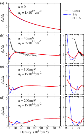
Figure 2: (Color online) $\frac{d\mu}{dn}$ for three different values of the band gap and impurity density for the diagrammatic perturbation theories. The points in panel (b) are taken from Fig. 2 of Ref. Henriksen and Eisenstein, 2010. Throughout, $\frac{d\mu}{dn}$ is given in units of $\mathrm{eV}\mathrm{nm}^{2}$.

In Fig. 2 we show the calculated $\frac{d\mu}{dn}$ for the clean case, Abergel (2012) the BA, and the SCBA as a function of the carrier density. The right-hand panels show the same data on a logarithmic scale to emphasize the low-density features. In the ungapped case shown in Fig. 2(a), the BA and SCBA give essentially the same result as the clean limit. When a band gap is present, as in Figs. 2(b) to 2(d), the clean limit shows a clear step occuring at the density $\tilde{n}=u^{2}/(v_{F}^{2}\pi)$ which marks the density where the chemical potential leaves the sombrero region of the band structure and the topology of the Fermi surface changes from a ring to a disk. Abergel et al. (2010) For $n\gg\tilde{n}$ the BA and SCBA are similar to the clean limit, but for low-to-moderate density $n\lesssim\tilde{n}$ the strong modification of the density of states (DOS) near the band edge Abergel et al. (2012) implies that $\frac{d\mu}{dn}$ is enhanced relative to the clean system but is still a decreasing function as $n$ becomes small. There is also a sharp divergence in the BA and SCBA for very small $n$ which is not observed experimentally. Henriksen and Eisenstein (2010); Young et al. (2010) Additional structure for $n<\tilde{n}$ in the BA comes from the non-trivial shape of the DOS near $\mu=u$ in that approximation, which is smoothed out by the self consistency of the SCBA. Abergel et al. (2012)

In Fig. 2(b) we also show experimental data for the gapped regime. Note that the data in Ref. Henriksen and Eisenstein, 2010 is a capacitance measurement, and in order to extract $\frac{d\mu}{dn}$ we need accurate knowledge of experimental parameters, such as the impurity density, the gate-induced band gap, the stray capacitance, and the dielectric environment, all of which are known only approximately. Therefore the experimental data shown here does not correspond to the parameters used in the calculation and hence we cannot expect quantitative agreement. Other experiments Young et al. (2010); Young and Levitov (2011) show the same qualitative features as in Ref. Henriksen and Eisenstein, 2010 although direct comparison to these data is not possible since the low-density $\frac{d\mu}{dn}$ is obscured by the specifics of the experimental setup used in these measurements. We see in Fig. 2(b) that a broad peak forms in the experimental data at low density in complete qualitative contrast to the BA and SCBA theoretical results. Therefore, these theories utterly fail to capture the essential physics of the gapped system at low densities. This is, however, not unexpected since the low density regime is completely dominated by the charged impurity induced random puddles of compressible and incompressible regions.

IV Thomas-Fermi theory

We now describe the TFT for the inhomogeneous system. In this approach, the carrier density landscape is obtained by minimizing a Thomas-Fermi energy functional of the spatially-varying density $n(\boldsymbol{\mathrm{r}})$ that includes a term due to the presence of disorder. The TFT is similar in spirit to the density functional theory (DFT) Hohenberg and Kohn (1964); Kohn and Sham (1965); Kohn (1999) but in TFT the kinetic energy operator is also replaced by a functional $E_{K}[n]$. This simplification makes the TFT valid only when the density profile varies on length scales larger than the Fermi wavelength, i.e., when $|\nabla n/n|<k_{F}$, where $k_{F}=\sqrt{\pi|n|}$ is the Fermi wave vector. This approach has been very successful in the context of transport calculations Das Sarma et al. (2011) which provides strong phenomenological support for the use of this theory. Specifically for bilayer graphene, the puddle length scale is $\sim 20\mathrm{nm}$ and the density of carriers in the puddles is $\sim 10^{12}\mathrm{cm}^{-2}$ so that this inequality is marginally satisfied. However, we can also justify this approximation by pointing out that the root-mean-square of the density distribution is much larger than its average. At the charge-neutrality point (CNP) the average density $n=0$ cannot be taken as a measure of the typical carrier density inside the puddles and a better estimate is given by $n_{\mathrm{rms}}$. As a consequence, at low dopings (close to the CNP) $n_{\mathrm{rms}}$ should be used instead of $n$ in the inequality above. Given that $n_{\mathrm{rms}}\sim n_{i}$ we then conclude that the TFT is valid at all densities so long as $n_{i}$ is not too small ($n_{i}>10^{11}\mathrm{cm}^{-2}$). A full DFT for the disordered problem has been completed for monolayer graphene Polini et al. (2008) and shows very similar results to the TFT applied in the same context. Rossi and Das Sarma (2008) However, the DFT is much more demanding of computational resources, and therefore it is not possible to simulate large lattice sizes or complete a comprehensive average over disorder realizations in a reasonable timescale. Moreover, given the difficulty to quantitatively compare the theoretical and experimental results (since parameters, such as the impurity density and stray capacitance, are not known accurately) and the complete failure of the diagrammatic methods to even achieve a gross qualitative description of the experimental results at low carrier density, our main motivation is to show that a functional method like the TFT is able to capture the qualitative features of the compressibility observed in experiments. The functional approach described below, notwithstanding the specifics of the TFT, is more than adequate to describe the compressibility of gapped systems in which the band gap is comparable to or smaller than the disorder strength.

The TFT energy functional is given by

$$E[n]=E_{K}[n(\boldsymbol{\mathrm{r}})]+\frac{e^{2}}{2\kappa}\int d\boldsymbol{\mathrm{r}}^{\prime}\int d\boldsymbol{\mathrm{r}}\frac{n(\boldsymbol{\mathrm{r}})n(\boldsymbol{\mathrm{r}}^{\prime})}{|\boldsymbol{\mathrm{r}}-\boldsymbol{\mathrm{r}}^{\prime}|}\\ +\frac{e^{2}}{\kappa}\int d\boldsymbol{\mathrm{r}}V_{D}(\boldsymbol{\mathrm{r}})n(\boldsymbol{\mathrm{r}})-\mu\int d\boldsymbol{\mathrm{r}}n(\boldsymbol{\mathrm{r}}),$$ (7)

where $e^{2}V_{D}/\kappa$ is the bare disorder potential which is assumed to be due to the Coulomb interaction with random charged impurities with no spatial correlation and an equal probability of being positively or negatively charged. The first term is the kinetic energy where

$$\epsilon_{K}[n(\boldsymbol{\mathrm{r}})]\equiv\frac{\delta E_{K}}{\delta n}=\begin{cases}\frac{1}{2}\sqrt{\frac{v_{F}^{4}\pi^{2}|n|^{2}+\gamma_{1}^{2}u^{2}}{\gamma_{1}^{2}+u^{2}}},&v_{F}^{2}\pi|n|<u^{2}\\ \sqrt{v_{F}^{2}\pi|n|+\frac{\gamma_{1}^{2}}{2}+\frac{u^{2}}{4}-\sqrt{v_{F}^{2}\pi|n|(\gamma_{1}^{2}+u^{2})+\frac{\gamma_{1}^{4}}{4}}},&u^{2}\leq v_{F}^{2}\pi|n|<2\gamma_{1}^{2}+u^{2}\\ \frac{1}{2}\sqrt{2v_{F}^{2}\pi|n|-u^{2}},&2\gamma_{1}^{2}+u^{2}\leq v_{F}^{2}\pi|n|\end{cases}$$ (8)

is the ground state kinetic energy per excess carrier. The second term is the Hartree part of the electron-electron interaction, the third term is the contribution due to the disorder potential, and in the fourth term $\mu$ is the chemical potential. We neglect exchange and correlation terms Borghi et al. (2010) since, as we shall show below, $\frac{d\mu}{dn}$ at low density is predominantly determined by the proportion of the sample which is incompressible and the inclusion of these terms will not change this. The ground state density landscape is identified by the equation $\delta E/\delta n=0$. Taking this variational derivative of $E[n]$, we find

$$\frac{\delta E}{\delta n}=\epsilon_{K}[n(\boldsymbol{\mathrm{r}})]+\frac{e^{2}}{2\kappa}\int d\boldsymbol{\mathrm{r}}^{\prime}\frac{n(\boldsymbol{\mathrm{r}}^{\prime})}{|\boldsymbol{\mathrm{r}}-\boldsymbol{\mathrm{r}}^{\prime}|}+\frac{e^{2}}{2\kappa}V_{D}(\boldsymbol{\mathrm{r}})-\mu.$$ (9)

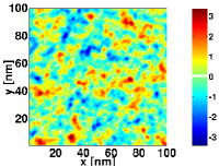
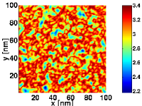
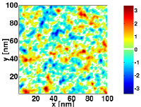
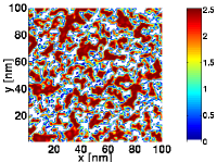
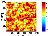
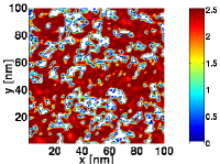
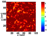
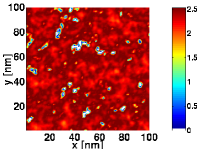
Figure 3: (Color online) (Left column) Spatial density profile, and (Right column) spatial $\frac{d\mu}{dn}$ profile for a single disorder realization. The units of the color bars are $10^{12}\mathrm{cm}^{-2}$ for the density and $\mathrm{eV}\,\mathrm{nm}^{2}$ for $\frac{d\mu}{dn}$, and $n_{i}=3\times 10^{11}\mathrm{cm}^{-2}$ throughout. The incompressible regions where $n=0$ are shown in white. The first row has $u=0$ and $\langle n\rangle=0$; the second row has $u=40\mathrm{meV}$ and $\langle n\rangle=0$; the third row has $u=40\mathrm{meV}$ and $\langle n\rangle\approx 2\times 10^{12}\mathrm{cm}^{-2}$; and the fourth row has $u=40\mathrm{meV}$ and $\langle n\rangle\approx 4\times 10^{12}\mathrm{cm}^{-2}$.

Within our formalism it is fairly easy to assume the presence of spatial correlations among the impurities, and the presence of correlations has important effects on the transport properties of BLG; Li et al. (2011); Yan and Fuhrer (2011); Li et al. (2012) however they do not modify the qualitative effects that the disorder has on the compressibility.

Assuming that the clean $\frac{d\mu}{dn}$ is valid locally, in Fig. 3 we show the spatial profile of the density distribution (left column) and $\frac{d\mu}{dn}$ (right column) for a single realization of disorder with $n_{i}=3\times 10^{11}\mathrm{cm}^{-2}$ for the gapless regime (first row) and the gapped case with $u=40\mathrm{meV}$ and three values of the global charge density. The white regions are the parts of the graphene where the local density is zero and hence the graphene is incompressible. It is immediately noticeable that in the presence of a band gap (second row) there are large incompressible regions which are not present in the gapless case (even at zero excess carrier density), and these regions persist even when the average charge density $\langle n\rangle$ is significant ($\langle n\rangle\approx 2\times 10^{12}\mathrm{cm}^{-2}$, third row) and are still just visible when $\langle n\rangle\approx 4\times 10^{12}\mathrm{cm}^{-2}$ (fourth row). More accurate functional methods than the TFT will not give substantially different values for the ratio of the sample that is covered by insulating (incompressible) regions, which we shall show is the dominant factor in determining $\frac{d\mu}{dn}$ at low density. All these methods can do is to give slightly different values of $n$ and density profiles inside metallic regions, both of which have very little influence on $\frac{d\mu}{dn}$ for the situation of interest.

By considering many disorder realizations we can calculate disorder averaged quantities and, in particular, the probability distribution function of the local carrier density $P(n)$. This function can then be used to compute the average density $\langle n\rangle=\int n^{\prime}P(n^{\prime})dn^{\prime}$. As shown in Fig. 4(a), $P(n)$ is trimodal for $\langle n\rangle=0$ in the gapped regime: it exhibits a large peak shown by an arrow at $n=0$ that quantifies the fraction of the sample ocupied by insulating regions and two smaller and broader peaks centered around values of $n$ which are determined by the nonlinear screening of the disorder potential and which therefore depend on both $u$ and $n_{i}$. Figure 4(a) also shows that $P(n)$ has a jump for $n=\tilde{n}$. As the doping increases, the fraction of the sample area covered by insulating regions $P(n=0)$ decreases as shown in Fig. 4(b). Notice the factor of $10^{3}$ difference in the vertical scale between Figs. 4(a) and 4(b). The evolution of $P(n)$ with $\langle n\rangle$ is shown in Fig. 4(c). For finite doping, the distribution becomes asymmetric in $n$ and becomes unimodal only at relatively large doping. In the unimodal regime, $P(n)$ is approximated closely by a Gaussian centered around $\langle n\rangle$.

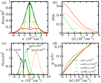
Figure 4: (Color online.) (a) $P(n)$ at the charge neutrality point $\langle n\rangle=0$ for different values of $u$ and $n_{i}$. For $u\neq 0$, the arrow at $n=0$ represents the very narrow peak whose height is orders of magnitude larger than the $y$-scale used. (b) $P(n=0)$ for parameters corresponding to Fig. 2(b) to 2(d). A dotted line at $P(0)=0.1$ provided as a guide to the eye. (c) Evolution of $P(n)$ with $\langle n\rangle$ for $u=40\mathrm{meV}$ and $n_{i}=3\times 10^{11}\mathrm{cm}^{-2}$. (d) $\mu$ as a function of doping. The legend in (d) also applies to panels (a) and (c).

Experimental probes such as the capacitance measurements and scanning SET microscopy, simultaneously probe an area of the sample which is significantly larger than the puddles size as predicted in the TFT and measured by STM. Zhang et al. (2009); Deshpande et al. (2009a); Xue et al. (2011); Deshpande et al. (2009b) Therefore, an averaging procedure must be implemented to replicate $\frac{d\mu}{dn}$ as a function of $\langle n\rangle$ as measured in those experiments. By disorder averaging the TFT results, we obtain the dependence of the average chemical potential $\langle\mu\rangle$ (which is identical to $\mu$ in Eq. (7)) with respect to the average density $\langle n\rangle$. Because of the non-linear screening, the relation between $\langle\mu\rangle$ and $\langle n\rangle$ is also modified by the value of the gap and the strength of the disorder, as shown in Fig. 4(d). Thus, the TFT results clearly show the inhomogeneous nature of the carrier density landscape in BLG in the presence of disorder. Using the TFT we calculate the average $\left\langle\frac{d\mu}{dn}\right\rangle=\frac{d\langle\mu\rangle}{d\langle n\rangle}$ which closely simulates the way in which $\langle d\mu/dn\rangle$ is obtained in both capacitance measurements Henriksen and Eisenstein (2010); Young et al. (2010); Young and Levitov (2011) and in SET spectroscopy. Martin et al. (2008, 2010)

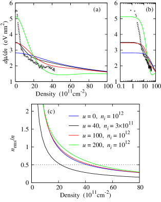
Figure 5: (Color online.) (a) The predicted $\frac{d\mu}{dn}$ in the TFT. (b) As in (a), but on a logarithmic scale to emphasize the low-density regime. (c) The density fluctuation due to disorder for the same parameters as in (a). The dotted line at $n_{n_{\mathrm{rms}}}/n=0.5$ is included as a guide to the eye.

Figure 5(a) shows the calculated $\frac{d\mu}{dn}$ using the TFT for the same four sets of parameters as in Fig. 2. We immediately see that it exhibits qualitatively different behavior from the BA and SCBA, and at low density it shows a broad peak in qualitative agreement with the experimental data. We stress that (as mentioned above) the data in Ref. Henriksen and Eisenstein, 2010 is the only appropriate data for direct comparison with our theories, but since various parameters of the experimental system are unknown, we cannot expect quantitative agreement between our calculations and the measured data. Comparison of Fig. 2 with Figs. 5(a) and 4(b) shows that the deviation of the perturbation theory from the TFT occurs when $P(0)>0.1$, indicating that the presence of insulating, incompressible regions is the dominating feature of the compressibility at low density. In Fig. 5(c) we show our TFT calculated density fluctuation characterized by the root-mean-square value $n_{\mathrm{rms}}$ as a function of density. This clearly establishes that, when a band gap is present and as the fluctuations (i.e. inhomogeneity) become large with decreasing average density, the calculated TFT results for $\frac{d\mu}{dn}$ start deviating substantially from the many-body perturbative ensemble averaged results, and when $n_{\mathrm{rms}}/n\approx 0.5$, one must carry out the nonlinear screening theory to obtain the qualitatively correct features for the compressibility.

V Discussion

Therefore, we identify two different reasons for the failure of the standard diagrammatic methods in gapped inhomogeneous systems. The first is the presence of strong inhomogeneity characterized by the parameter $n_{\mathrm{rms}}/n$. When $n_{\mathrm{rms}}/n>a$ with $a\sim 1$, the ground state cannot be assumed to be homogeneous and therefore implicit translational invariance incorporated in the disorder averaging step of the diagrammatic theory fails to qualitatively describe the experimental situation. The exact value of $a$ depends on the experimental quantity under consideration and the details of the experimental conditions. The second reason for failure is the existence of a random mixed inhomogeneous state where insulating (incompressible) and metallic (compressible) regions coexist in the presence of a band gap of the order of or smaller than the disorder strength. The diagrammatic methods fail because they cannot account for this mixed state. For the compressibility, comparison of Fig. 4(b) with Fig. 2 shows that the critical fraction of the sample area to be covered by insulating regions for the perturbative theories to give strong qualitative disagreement with the experiments is $P(0)>0.1$. Thus, disorder has a much stronger qualitative effect at low carrier densities for gapped bilayer graphene Henriksen and Eisenstein (2010); Martin et al. (2010) than for the monolayer Martin et al. (2008) since BLG, by virtue of being a gapped system, can be in the random mixed state which is not accessible for ungapped systems.

In conclusion, we have demonstrated that the nonlinear nature of the screening of an external disorder potential in gapped bilayer graphene and the resulting charge inhomogeneity are crucial in understanding the ground state electronic properties for a wide range of experimentally relevant carrier densities. In particular, standard many-body diagrammatic techniques assume that the density profile is homogeneous in both the screening and the Green’s function, and therefore give qualitatively incorrect predictions for the compressibility in the presence of an external band gap. In contrast, the TFT retains the inhomogeneity and non-linear screening of the density distribution in the energy functional $E[n(\boldsymbol{\mathrm{r}})]$ and therefore captures the essential physics of the system. We emphasize that this particular averaging procedure discussed in Sec. IV, simulating the experimental conditions, is simply inaccessible to any type of theories invoking a homogeneous charge landscape to obtain many-body self-energy or broadening. We also point out that although we have presented results where the disorder potential is induced by random charged impurities, our general conclusion will remain valid for any form of disorder which produces a scalar potential perturbation to the clean Hamiltonian, such as corrugations in the graphene sheet. Gibertini et al. (2012) Finally, although we have described calculation of the compressibility (and equivalently $\frac{d\mu}{dn}$) the general logic of our argument applies to other observable quantities also. For instance, application of the Kubo formula for transport with Green’s functions derived in the same way as in Sec. III will suffer from similar problems in the inhomogeneous regime. In this example, an effective medium theory Rossi et al. (2009) or a full quantum transport analysis that explicitly takes into account the inhomogeneities Rossi et al. (2012) should be used instead.