Carbon-rich dust production in metal-poor galaxies in the Local Group

Abstract

We have observed a sample of 19 carbon stars in the Sculptor, Carina, Fornax, and Leo I dwarf spheroidal galaxies with the Infrared Spectrograph on the Spitzer Space Telescope. The spectra show significant quantities of dust around the carbon stars in Sculptor, Fornax, and Leo I, but little in Carina. Previous comparisons of carbon stars with similar pulsation properties in the Galaxy and the Magellanic Clouds revealed no evidence that metallicity affected the production of dust by carbon stars. However, the more metal-poor stars in the current sample appear to be generating less dust. These data extend two known trends to lower metallicities. In more metal-poor samples, the SiC dust emission weakens, while the acetylene absorption strengthens. The bolometric magnitudes and infrared spectral properties of the carbon stars in Fornax are consistent with metallicities more similar to carbon stars in the Magellanic Clouds than in the other dwarf spheroidals in our sample. A study of the carbon budget in these stars reinforces previous considerations that the dredge-up of sufficient quantities of carbon from the stellar cores may trigger the final superwind phase, ending a star’s lifetime on the asymptotic giant branch.

1. Introduction

Stars on the asymptotic giant branch (AGB) are an important source of dust injected into the interstellar medium in the Milky Way (e.g., Gehrz, 1989; Habing, 1996). How important they are in more metal-poor environments is an open question, with consequences for the early history of the Milky Way, current conditions in other smaller Local Group galaxies, and even for galaxies in the high-redshift Universe.

The sensitivity of the Infrared Spectrograph (IRS; Houck et al., 2004) on the Spitzer Space Telescope (Werner et al., 2004) has made it possible to explore this question by observing the dust forming around individual evolved stars in environments spanning a range of metallicities, both in our own galaxy and elsewhere in the Local Group. The IRS has observed dust around AGB stars in the Large Magellanic Cloud (LMC; Zijlstra et al., 2006; Buchanan et al., 2006; Leisenring et al., 2008), Small Magellanic Cloud (SMC; Sloan et al., 2006; Lagadec et al., 2007), Fornax Dwarf Spheroidal (Matsuura et al., 2007), Sagittarius Dwarf Spheroidal (Lagadec et al., 2009), Sculptor Dwarf Spheroidal (Sloan et al., 2009), and several Galactic globular clusters (Lebzelter et al., 2006; Sloan et al., 2010; McDonald et al., 2011). These metalliticies of these systems span a range of $-$2.1 $<$ [Fe/H] $<$ 0.0. Comparisons of these samples with each other and with samples from the Galactic disk reveal that the amount of dust produced around oxygen-rich AGB stars decreases in more metal-poor environments (Sloan et al., 2008, 2010), but for carbon-rich AGB stars, the amount of dust observed shows no measurable dependence on metallicity (Matsuura et al., 2007; Groenewegen et al., 2007; Sloan et al., 2008).

Stars on the AGB will produce either carbon-dominated or oxygen-dominated dust, depending on their dredge-up histories and initial abundances. AGB stars generate carbon via the triple-alpha sequence (Salpeter, 1952) in a helium-burning shell around an inert C/O core (e.g., Iben & Renzini, 1983). The helium fusion proceeds in a series of thermal pulses in the interior, leading to pulses of convection which dredge newly produced carbon up to the surface. The dredge-ups can raise the photospheric C/O ratio above unity, converting an AGB star with a spectral class of M giant to a carbon star. The envelopes of AGB stars are unstable to pulsations with typical periods of hundreds of days, making them readily identifiable as long-period variables (LPVs). These pulsations in the envelopes may even drive the mass-loss process (see Mattsson et al., 2008, and references therein).

The formation of CO in the resulting outflows will exhaust all of the available carbon or oxygen, whichever is less abundant, leading to a chemical dichotomy in the dust which will condense out of the outflowing gas. Alumina and silicates will dominate the shells around M giants, and amorphous carbon will dominate the shells around carbon stars (e.g., Martin & Rogers, 1987; Onaka et al., 1989; Egan & Sloan, 2001).

In more metal-poor galaxies, stars of lower initial mass will become carbon stars on the AGB. Counts of carbon stars in the LMC and SMC reveal this fact observationally (Blanco et al., 1978, 1980; Cioni & Habing, 2003), and it is expected theoretically (Renzini & Voli, 1981; Karakas & Lattanzio, 2007). A recent infrared census of the SMC with Spitzer reveals the consequence: carbon stars produce more dust than their oxygen-rich AGB counterparts or red supergiants (Matsuura, 2012), possibly much more (Boyer et al., 2012). The SMC serves as a proxy for metal-poor galaxies too distant for their constituent stars to be studied individually. By studying even more metal-poor galaxies in the Local Group, we can push to even more primitive systems.

The infrared spectra of seven carbon stars beyond the Magellanic Clouds have been published so far, six in Fornax (Matsuura et al., 2007), and one in Sculptor (Sloan et al., 2009). This paper presents spectra from the IRS for a larger sample of carbon stars in these two galaxies, as well as the Carina and Leo I dwarf spheroidal (dSph) galaxies. The stars in the sample are quite faint in the infrared, and the development of a new algorithm to extract spectra from the two-dimensional IRS images (Lebouteiller et al., 2010) makes it possible to analyze their spectra similarly to closer and brighter samples. Additionally, near-infrared (NIR) monitoring from the South African Astronomical Observatory (SAAO) has provided information on the pulsation modes and periods of the targeted stars which was not available when Spitzer observed them. These two improvements give us the opportunity to extend the previous comparisons of mass loss and dust production in evolved stars to more distant galaxies with lower metallicities.

Section 2 presents our targeted galaxies, with an emphasis on their distances and metallicities, and explains how we selected our sample of stars. Section 3 describes the observations and data reduction. In Section 4, we determine bolometric magnitudes and use these to re-assess the metallicities. Section 5 presents the spectroscopic results, and Section 6 discusses the consequences of our findings.

2. The sample

2.1. Target galaxies

Table 1Dwarf Spheroidal Galaxies Studied

dSph	Distance	Adopted	Mean	Adopted
galaxy	modulus	$E(B-V)$	[Fe/H]	[Fe/H]
Sculptor	19.64 $\pm$ 0.04	0.02	$-$1.56 $\pm$ 0.40	$\sim$$-$1.0
Carina	20.10 $\pm$ 0.04	0.025	$-$1.73 $\pm$ 0.35	$-$1.73
Fornax	20.74 $\pm$ 0.07	0.025	$-$0.99 $\pm$ 0.44	$-$0.3 to $-$0.8
Leo I	22.07 $\pm$ 0.07	0.03	$-$1.35 $\pm$ 0.24	$-$1.35

Table 2Distances to the Galaxies

Galaxy	Distance	Ref.
	modulus
Sculptor	19.71 $\pm$ 0.10	Kaluzny et al. (1995)
	19.64 $\pm$ 0.04	Rizzi et al. (2007a)
	19.67 $\pm$ 0.12	Pietryzyński et al. (2008)
Carina	20.09 $\pm$ 0.06	Smecker-Hane et al. (1994)
	20.06 $\pm$ 0.12	Mateo et al. (1998)
	20.19 $\pm$ 0.12	Dall’Ora et al. (2003)
	20.11 $\pm$ 0.13	Pietryzyński et al. (2009) (avg. of $J$, $K$)
Fornax	20.76 $\pm$ 0.10	Buonanno et al. (1999)
	20.70 $\pm$ 0.12	Saviane et al. (2000) (tip of RGB)
	20.76 $\pm$ 0.04	Saviane et al. (2000) (HB)
	20.65 $\pm$ 0.11	Bersier (2000)
	20.86 $\pm$ (0.04)	Pietryzyński et al. (2003)
	20.66 $\pm$ (0.04)	Mackey & Gilmore (2003)
	20.64 $\pm$ 0.09	Greco et al. (2007)
	20.72 $\pm$ 0.04	Rizzi et al. (2007b)
	20.75 $\pm$ 0.19	Gullieuszik et al. (2007) (tip of RGB)
	20.75 $\pm$ 0.11	Gullieuszik et al. (2007) (red clump)
	20.84 $\pm$ 0.14	Pietryzyński et al. (2009)
Leo I	22.18 $\pm$ 0.11	Lee et al. (1993)
	22.00 $\pm$ 0.15	Caputo et al. (1999)
	22.04 $\pm$ 0.14	Held et al. (2001)
	22.05 $\pm$ 0.18	Méndez et al. (2002)
	22.02 $\pm$ 0.13	Bellazzini et al. (2004)
	22.04 $\pm$ 0.11	Held et al. (2010)

Our targets sample the evolved stellar population in four dwarf spheroidal galaxies in the Local Group. Sculptor was the first dwarf spheroidal discovered, quickly followed by Fornax (Shapley, 1938). Leo I was uncovered during the first Palomar Sky Survey (Harrington & Wilson, 1950), and Cannon et al. (1977) detected the Carina dwarf while conducting the Southern Sky Survey from the European Southern Observatory (ESO). Table 1 presents some basic data for these galaxies that we will use for the remainder of the paper, and it requires some explanation.

The distance moduli were determined with weighted averages of published distances based on standard candles such as RR Lyrae variables, the horizontal branch (HB), and the tip of the red giant branch (RGB). The uncertainties in the distance moduli are statistical and do not reflect systematic errors, which are likely to be larger. Table 2 lists the individual distance measurements used to determine the results in Table 1. The entries in Table 2 are not meant to be exhaustive; some measurements rendered redundant or obsolete by more recent work are not included. Uncertainties smaller than 0.04 magnitudes have been raised to that limit for the purpose of weighting (and noted with parentheses in Table 2).

Table 1 includes our assumed values of interstellar reddening from foreground extinction in the Galaxy, $E(B-V)$. In this study, they only influence our derived bolometric magnitudes, and the influence is small, because the extinction is small to begin with and smaller still in the NIR, where the carbon stars emit most of their energy. As an example, a reddening of 0.03 magnitudes corresponds to an extinction of 0.03 magnitudes at $J$ and 0.01 at $K$ (using the extinction law of Rieke & Lebofsky, 1985), making the impact of reddening smaller than our uncertainty in distance. Our assumed reddening values are consistent with the literature and the infrared dust maps of Schlegel et al. (1998), except that reddening derived from the dust maps is higher than typical values used for Carina (0.06 vs. 0.025 mag.; e.g., Smecker-Hane et al., 1994; Mateo et al., 1998).

2.2. Metallicities

Our objective is to understand how the infrared spectral characteristics of carbon stars vary with metallicity, making it important that we understand the metallicity distribution functions (MDFs) of the parent populations of our targeted carbon stars in each galaxy. Tackling this question is not easy, given the complex star formation histories of these systems. Each galaxy is unique in this regard.

2.2.1 Sculptor

Sculptor has two populations with different ages, metallicities, and spatial distributions. Its color-magnitude diagram (CMD) shows two RGB bumps and two HBs, consistent with two populations with distinct metallicities (Majewski et al., 1999). Hurley-Keller et al. (1999) noticed that the red HB, which arises from the more metal-rich population, is confined to the center of the galaxy.

In the past decade, multiple studies have used the Fibre Large Multi-Element Spectrograph (FLAMES) at the Very Large Telescope (VLT), measuring the Ca II triplet (CaT) at 0.85 $\mu$m to determine the metallicity of hundreds of RGB stars. Those that focus on the core regions (within $\sim$10–15$\arcmin$ of the center) tend to produce more metal-rich MDFs compared to those sampling larger parts of the galaxy. Inside 12$\arcmin$ of the center, Tolstoy et al. (2004) find a MDF with $<$[Fe/H]$>$ = $-$1.49 $\pm$ 0.35, but outside that ellipsoidal radius, $<$[Fe/H]$>$ = $-$1.91 $\pm$ 0.27 (our calculations based on figures in their paper; all metallicities are on the CG97 scale from Carretta & Gratton, 1997). Similarly, Kirby et al. (2009) find $<$[Fe/H]$>$ = $-$1.58 $\pm$ 0.41 for a large sample within 10$\arcmin$ of the center, while Helmi et al. (2006) find $<$[Fe/H]$>$ = $-$1.82 $\pm$ 0.34 for a sample out to the tidal radius (76$\farcm$5; our $<$[Fe/H]$>$ calculation based on their data).

Revaz et al. (2009) explain this dichotomy with a young, metal-rich population (age $\lesssim$ 2 Gyr), and an old metal-poor population (age $\gtrsim$ 9 Gyr). Their models indicate no intermediate-age population. Our carbon stars are more likely to belong to the younger population (see § 4.2), which corresponds to the population dominating the core of the galaxy. To approximate the metallicity in the core, we have averaged the inner sample defined by Tolstoy et al. (2004) and the sample of Kirby et al. (2009), weighting by sample size (97 and 393, respectively), to arrive at an estimated $<$[Fe/H]$>$ of $-$1.56 $\pm$ 0.40. However, this value is too metal-poor compared to the metallicity of the younger population according to the models of Revaz et al. (2009), leading us to revise the metallicity in § 4.2.

2.2.2 Carina

Carina has experienced multiple, discrete star-formation events (Mighell, 1990). Smecker-Hane et al. (1996) detected three main-sequence turn-off points, along with three locations for helium-burning stars (two HBs and a red clump projected onto the RGB), which Hurley-Keller et al. (1998) dated to three star-formation events early in the galaxy’s history and $\sim$7 and $\sim$3 Gyr ago. This basic scenario has stood the test of another decade of observations (e.g., Monelli et al., 2003; Bono et al., 2010, and references therein). Models by Revaz et al. (2009) suggest that the intermediate population formed in a series of several bursts.

Despite this complex star-formation history, Carina shows a relatively shallow metallicity gradient (Walker et al., 2009) and a MDF no broader than that of Sculptor. CaT observations with VLT/FLAMES by Helmi et al. (2006) cover Carina out to $\sim$36$\arcmin$, and from their data we determine that $<$[Fe/H]$>$ = $-$1.81 $\pm$ 0.31. Other recent estimates are $-$1.72 $\pm$ 0.39 (Koch et al., 2006), $-$1.69 $\pm$ 0.51 (Koch et al., 2008), and $-$1.70 $\pm$ 0.19 (Bono et al., 2010). The mean of these results is $-$1.73 $\pm$ 0.35 (we have averaged the available uncertainties).

2.2.3 Fornax

Fornax has experienced a steadier rate of star formation over the past several Gyr compared to Sculptor and Carina, resulting in a broader MDF. The CMD of Fornax has a wide RGB (Demers et al., 1979), which requires a range of metallicities and/or ages. Fornax contains many carbon stars, proof of a substantial population of intermediate-age stars (Demers & Kunkel, 1979; Aaronson & Mould, 1980). Further study made it apparent that episodes of star formation have continued to within the last few hundred Myr (Aaronson & Mould, 1985; Buonanno et al., 1985, 1999), and that younger stars are more concentrated in the core of the galaxy (Stetson et al., 1998). More recent work has largely confirmed these earlier findings (e.g., Tolstoy et al., 2001; Pont et al., 2004; Helmi et al., 2006).

CaT observations in large samples of RGB stars by Battaglia et al. (2006) trace the metallicity gradient in Fornax. They find a MDF within 24$\arcmin$ of the center with $<$[Fe/H]$>$ = $-$0.99 $\pm$ 0.44, compared to $-$1.52 $\pm$ 0.46 outside 42$\arcmin$ of the center (the quoted quantities are our determinations from their data). A study of CMDs within Fornax by Coleman & de Jong (2008) support the spectroscopic results. Our sample of carbon stars mostly conforms to the innermost sample considered by Battaglia et al. (2006), and we will adopt $-$0.99 as a starting metallicity for consideration.

However, models by Revaz et al. (2009) suggest that the carbon stars could be significantly more metal-rich; most of the stars formed in the past few Gyr should have [Fe/H] in the range from $\sim$ $-$0.3 to $-$0.8, which would make these carbon stars more similar to those in the LMC and SMC than in the other three dwarf spheroidal galaxies in our sample. We return to this point in § 4.2 below.

2.2.4 Leo I

Leo I is the most distant of the dwarf galaxies in the Milky Way system of the Local Group. In fact, it is unclear whether or not it is gravitationally bound to the Local Group (e.g., Lépine et al., 2011). Its distance and its proximity to Regulus have made observations more challenging than for the other dwarfs considered here. Nonetheless, a picture has emerged of a galaxy with the contradictory properties of a relatively young population and relatively metal-poor abundances (Lee et al., 1993). The majority of the visible stars in the galaxy appear to have formed 3–7 Gyr ago (Demers et al., 1994) or 1–7 Gyr ago (Gallart et al., 1999).

Despite the ongoing star formation, gradients in the population are subtle (Gullieuszik et al., 2009; Held et al., 2010), and the metallicity shows a fairly narrow and well-defined distribution. CaT spectra give $<$[Fe/H]$>$ values of $-$1.34 $\pm$ 0.26 (102 stars; Bosler et al., 2007), $-$1.31 $\pm$ 0.25 (58 stars; Koch et al., 2007), and $-$1.41 $\pm$ 0.21 (54 stars; Gullieuszik et al., 2009). Combining these results and weighting by their sample size yields $<$[Fe/H]$>$ = $-$1.35 $\pm$ 0.24.

2.3. Stellar samples

Table 3Targets

Source	Position (J2000)		2MASS photometry			Other
name	RA	Dec.	$J$	$H$	$K_{s}$	designations
MAG 29	00 59 53.67	$-$33 38 30.8	14.846 $\pm$ 0.038	13.144 $\pm$ 0.031	11.603 $\pm$ 0.021
Scl V78 V544	00 59 58.94	$-$33 28 35.2	13.399 $\pm$ 0.021	12.633 $\pm$ 0.025	12.273 $\pm$ 0.023	ALW Scl 3
For BW 2	02 38 06.19	$-$34 31 19.4	16.052 $\pm$ 0.104	14.483 $\pm$ 0.055	13.315 $\pm$ 0.048	GLM 31
For BTH 13-23	02 38 50.56	$-$34 40 32.0	16.106 $\pm$ 0.094	14.525 $\pm$ 0.053	12.879 $\pm$ 0.029
For BTH 12-4	02 39 12.33	$-$34 32 45.0	14.722 $\pm$ 0.033	13.262 $\pm$ 0.038	12.120 $\pm$ 0.024	GLM 25
For BTH 3-129	02 39 41.60	$-$34 35 56.7	$\cdots$	15.970 $\pm$ 0.205	14.164 $\pm$ 0.070
For DK 18	02 39 54.21	$-$34 38 36.9	15.601 $\pm$ 0.064	14.162 $\pm$ 0.049	13.167 $\pm$ 0.033	GLM 24
For DK 52	02 40 06.66	$-$34 23 22.3	14.485 $\pm$ 0.029	13.377 $\pm$ 0.034	12.618 $\pm$ 0.027	DDB 17, GLM 13
For DI 2	02 40 09.47	$-$34 06 25.7	15.790 $\pm$ 0.075	14.556 $\pm$ 0.068	13.668 $\pm$ 0.052	GLM 16
For WEL C10	02 40 10.17	$-$34 33 21.9	14.063 $\pm$ 0.026	13.122 $\pm$ 0.021	12.545 $\pm$ 0.029	DI 20, SHS 105, BW 62, DDB 19, BTH 4-25
For BW 69	02 40 17.79	$-$34 27 35.8	15.424 $\pm$ 0.063	14.122 $\pm$ 0.049	13.182 $\pm$ 0.035	GLM 21
For BW 75	02 40 31.23	$-$34 28 44.2	14.745 $\pm$ 0.043	13.689 $\pm$ 0.046	13.072 $\pm$ 0.037	DDB 22, BTH 6-13, GLM 17
For BW 83	02 41 03.56	$-$34 48 05.4	14.441 $\pm$ 0.035	13.365 $\pm$ 0.034	12.694 $\pm$ 0.034	DDB 25, MAG 30, GLM 27
ALW Car 2	06 41 13.53	$-$50 54 25.0	13.925 $\pm$ 0.024	13.073 $\pm$ 0.028	12.658 $\pm$ 0.027
Car MCA C3	06 41 41.45	$-$50 58 08.1	13.742 $\pm$ 0.022	12.805 $\pm$ 0.023	12.340 $\pm$ 0.026	ALW Car 6
Car MCA C5	06 42 10.35	$-$50 56 24.0	13.940 $\pm$ 0.023	13.159 $\pm$ 0.027	12.785 $\pm$ 0.029	ALW Car 10
Leo I MFT C	10 08 22.25	$+$12 17 57.1	$\cdots$	16.195 $\pm$ 0.214	14.225 $\pm$ 0.060	HGR 8717
Leo I MFT A	10 08 29.28	$+$12 18 51.6	17.134 $\pm$ 0.202	15.429 $\pm$ 0.103	14.025 $\pm$ 0.053	HGR 6343
Leo I MFT E	10 09 00.5	$+$12 19 01	$\cdots$	$\cdots$	$\cdots$

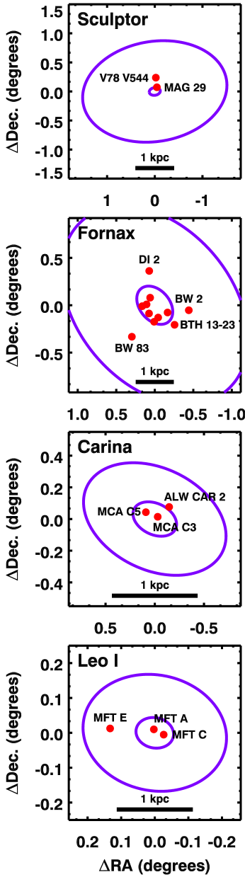
Figure 1.— The locations of our targets within each galaxy. The ellipses are the tidal and core radii defined by Irwin & Hatzidimitriou (1995). In Fornax, only the sources outside of the core are labelled.

Table 4Optical photometry

Source	Photometry				Ref.
name	$B$	$V$	$R$	$I$
MAG 29	$\cdots$	$\cdots$	20.22	18.04	USNO-B
Scl V78 V544	20.20	16.55	16.53 $\pm$ 0.49	16.70	USNO-B
For BW 2	$\cdots$	20.23 $\pm$ 0.07	19.21 $\pm$ 1.58	16.47 $\pm$ 0.05	BW, USNO-B
For BTH 13-23	$\cdots$	$\cdots$	$\cdots$	$\cdots$
For BTH 12-4	$\cdots$	$\cdots$	$\cdots$	$\cdots$
For BTH 3-129	$\cdots$	$\cdots$	$\cdots$	$\cdots$
For DK 18	21.45	18.57 $\pm$ 0.60	17.51 $\pm$ 1.46	16.01	DK, USNO-B
For DK 52	22.06	19.74 $\pm$ 0.33	17.93 $\pm$ 0.51	18.15	DK, WEL, USNO-B
For DI 2	21.4	18.3 $\pm$ 0.7	17.07 $\pm$ 0.42	16.75	WEL, DI, USNO-B
For WEL C10	22.31 $\pm$ 0.03	19.41 $\pm$ 0.05	18.24 $\pm$ 1.08	15.73 $\pm$ 0.04	SHS, BW, USNO-B
For BW 69	21.93	19.99 $\pm$ 0.05	19.80 $\pm$ 0.74	16.64 $\pm$ 0.04	BW, USNO-B, GSC
For BW 75	20.63	20.06 $\pm$ 0.03	18.14 $\pm$ 0.33	16.99 $\pm$ 0.07	GSC, BW, USNO-B
For BW 83	23.26	20.41 $\pm$ 0.10	17.63 $\pm$ 0.98	16.62 $\pm$ 0.06	BW, USNO-B, NOMAD
ALW Car 2	18.89 $\pm$ 0.64	17.64	16.37 $\pm$ 0.01	15.64	USNO-B, NOMAD, K06
Car MCA C3	18.43	17.48	15.86	15.27	USNO-B, NOMAD
Car MCA C5	18.95 $\pm$ 0.71	17.26 $\pm$ 0.09	16.01 $\pm$ 0.33	15.11	M82, USNO-B, NOMAD
Leo I MFT C	$\cdots$	$\cdots$	$\cdots$	$\cdots$
Leo I MFT A	$\cdots$	$\cdots$	$\cdots$	$\cdots$
Leo I MFT E	$\cdots$	$\cdots$	$\cdots$	$\cdots$

The carbon stars in our sample were observed in two Spitzer programs. The first, a Cycle 2 program, included five carbon stars in Fornax (published by Matsuura et al., 2007) and three carbon-star candidates in Leo I. The second program followed in Cycle 3 and included six carbon stars in Fornax, three in Carina, and two in Sculptor. Sloan et al. (2009) published one of the two Sculptor spectra. Table 3 gives the names, positions, and NIR fluxes from 2MASS (Skrutskie et al., 2006) of the stars in our sample. Figure 1 shows where our targets are located in each galaxy.

Fornax is well known as an abundant source of carbon stars, starting with the initial detection of several candidates by Demers & Kunkel (1979) and the spectroscopic confirmation of six by Aaronson & Mould (1980). By 1999, the number of confirmed carbon stars had climbed to 104 (Azzopardi et al., 1999). Multiple programs have searched Fornax for LPVs. Demers & Irwin (1987) found 30 candidates, but no Mira variables. Bersier & Wood (2002) identified 85 candidates, but did not attempt to determine periods. Whitelock et al. (2009) published the results of a thorough NIR monitoring program from the SAAO. The Cycle 2 program selected five targets in Fornax based on the SAAO observations, although at that time the mean NIR magnitudes and periods were not known. The six targets in Cycle 3 were selected based on 1–5 $\mu$m spectra and photometry with the Infrared Spectrometer and Array Camera (ISAAC) on the VLT. Groenewegen et al. (2009a) published the results of these observations, which include eight of our 11 targets. The combination of the various observations confirms that all of our sample are carbon-rich. The SAAO photometry provides periods for six of our 11 targets in Fornax. Four of these are Mira variables, while two are semi-regulars.

Our search for targets in Sculptor began with the 2MASS survey. Two targets fulfilled our criteria that $J-K_{s}>1.1$ and $K_{s}<$ 12.5. V78 V544 was originally identified as a LPV by van Agt (1978). This star had the reddest $J-K$ color (1.19) in the study by Frogel et al. (1982), but they were unable to determine if it was carbon-rich spectroscopically. Azzopardi et al. (1986) made that confirmation, noting that their list of eight carbon stars was likely to be complete. However, the optical surveys in use at that time missed the sources embedded in the most optically thick shells. Our other Sculptor target, MAG 29, has $J-K_{s}=3.24$. Mauron et al. (2004) first noticed this source in their search of 2MASS targets in the direction of several dwarf galaxies, but they estimated its distance to be $\sim$50 kpc, in the foreground of the Sculptor dwarf. Sloan et al. (2009) published an early version of the IRS spectrum of MAG 29. Using two different infrared color-magnitude relations, they estimated its distance to be 84 $\pm$ 13 kpc, consistent with the distance of Sculptor in Table 1, 85 $\pm$ 2 kpc. Near-infrared spectra of V78 V544 and MAG 29 by Groenewegen et al. (2009a) confirm their carbon-rich nature. Menzies et al. (2011) find that both are Mira variables and that the P-L relation gives distances for these two consistent with membership in Sculptor.

We also used the 2MASS survey to search Carina for suitable targets. Four sources fulfilled the criteria $J-K_{s}>$ 1.1 and $K_{s}<$ 13.0 (excluding obvious foreground sources), and of these we observed three. Mould et al. (1982) originally identified two of our three targets as carbon stars, and we adopt their names for them. Azzopardi et al. (1986) included all four of the red sources in their list of nine spectroscopically confirmed carbon stars in Carina. They stated that the list should be complete for the area observed.

More carbon stars have been detected in Leo I than in Sculptor or Carina. Azzopardi et al. (1986) listed 16 spectroscopically confirmed carbon stars and two candidate carbon stars in Leo I. However, none of these are very red. A more recent NIR survey from the SAAO detected five highly reddened stars with $J-K_{s}>$ 2 (Menzies et al., 2002). In our Cycle 2 program, we observed the three reddest, all with $J-K_{s}>$ 3. Menzies et al. (2010) determined periods for our three Leo I targets as part of a larger effort which identified 26 AGB variables in the galaxy from the SAAO. While it is quite likely that all three of our targets are carbon-rich, the spectra presented here are our first chance to confirm their chemistry.

Table 5Variability

Source	Var.	Period	Photometry						Ref.
name	class	(days)	$J$	$\Delta J$	$H$	$\Delta H$	$K_{s}$	$\Delta K_{s}$
MAG 29	Mira	554	14.35		12.94		11.44	0.87	M11
Scl V78 V544	Mira	189	13.78		12.90		12.38	0.42	M11
For BW 2	var.	$\cdots$	16.05 $\pm$ 0.10		14.48 $\pm$ 0.06		13.32 $\pm$ 0.05		BW, 2MASS
For BTH 13-23	Mira	350	17.09	1.28	15.33	1.24	13.63	1.02	W09
For BTH 12-4	Mira	470	16.01	1.44	14.31	1.14	12.91	0.96	W09
For BTH 3-129	Mira	400	18.00	1.64	15.83	1.43	13.90	1.16	W09
For DK 18	var.	$\cdots$	14.71	1.00	13.59	0.76	12.78	0.43	W09
For DK 52	var.	$\cdots$	14.76	0.61	13.60	0.52	12.80	0.32	W09
For DI 2	irr.	$\cdots$	15.79 $\pm$ 0.07		14.56 $\pm$ 0.07		13.67 $\pm$ 0.05		DI, 2MASS
For WEL C10	SR	317	15.09	0.64	13.87	0.43	13.05	0.26	DI, W09
For BW 69	SR	340	16.24		14.85		13.61		W09
For BW 75	var.	$\cdots$	15.12	1.00	13.94	0.75	13.16	0.51	W09
For BW 83	Mira	280	14.87	0.69	13.77	0.56	12.99	0.52	W09
ALW Car 2	var.	$\cdots$	13.93 $\pm$ 0.03		13.07 $\pm$ 0.03		12.66 $\pm$ 0.03		SAAO, 2MASS
Car MCA C3	var.	$\cdots$	13.74 $\pm$ 0.03		12.81 $\pm$ 0.02		12.34 $\pm$ 0.03		SAAO, 2MASS
Car MCA C5	var.	$\cdots$	13.94 $\pm$ 0.03		13.16 $\pm$ 0.03		12.79 $\pm$ 0.03		SAAO, 2MASS
Leo I MFT C	Mira	523	17.46	1.52	15.68	1.29	13.98	1.03	M10
Leo I MFT A	Mira	336	17.62	1.23	15.88	1.01	14.39	0.81	M10
Leo I MFT E	Mira	283	19.18	1.87	17.25	1.23	15.63	1.17	M10

Table 4 gives the best available optical photometry for the sources in our sample. Entries in bold are average magnitudes and the standard deviations when the quoted sources give multiple measurements or provide a mean. Table 5 presents variability classes, periods, and NIR photometry. The entries in bold in this table are mean magnitudes and peak-to-peak amplitudes published by the SAAO (references are given in the table notes).

3. Observations and data reduction

Table 6IRS observations

Source	AOR	Program	Observing date		On-source integration times (sec)
name	key		day	JD$-$2400000.5	SL2	SL1	LL2	LL1
MAG 29	18050816	30333	2006 Dec 19	54088.9	240	240	960	960
Scl V78 V544	18051072	30333	2006 Dec 20	54089.1	2880	5280	$\cdots$	$\cdots$
For BW 2	18053376	30333	2007 Feb 08	54139.7	480	480	2880	2880
For BTH 13-23	14540544	20357	2006 Jan 30	53765.6	2880	3360	$\cdots$	$\cdots$
For BTH 12-4	14541056	20357	2006 Jan 27	53762.9	2880	3360	$\cdots$	$\cdots$
For BTH 3-129	14540800	20357	2006 Jan 30	53765.5	2880	3360	$\cdots$	$\cdots$
For DK 18	18052864	30333	2007 Feb 08	54139.6	1440	1440	$\cdots$	$\cdots$
For DK 52	18052096	30333	2006 Dec 19	54088.9	1440	1440	$\cdots$	$\cdots$
For DI 2	18052352	30333	2007 Feb 06	54137.6	2880	2880	$\cdots$	$\cdots$
For WEL C10	14541824	20357	2006 Jan 27	53762.9	2880	3360	$\cdots$	$\cdots$
For BW 69	18052608	30333	2007 Feb 07	54138.9	1440	1440	$\cdots$	$\cdots$
For BW 75	14542080	20357	2006 Jan 27	53762.8	2880	3360	$\cdots$	$\cdots$
For BW 83	18053120	30333	2007 Feb 08	54139.7	1440	1440	$\cdots$	$\cdots$
ALW Car 2	18051584	30333	2007 Mar 12	54171.9	2880	5280	$\cdots$	$\cdots$
Car MCA C3	18051328	30333	2007 Mar 12	54171.8	2880	4800	$\cdots$	$\cdots$
Car MCA C5	18051840	30333	2007 Mar 13	54172.0	3840	5760	$\cdots$	$\cdots$
Leo I MFT C	14545152	20357	2006 May 25	53880.0	2880	3360	$\cdots$	$\cdots$
Leo I MFT A	14545408	20357	2006 May 25	53880.1	2880	3360	$\cdots$	$\cdots$
Leo I MFT E	14545920	20357	2006 May 25	53880.2	2880	3120	$\cdots$	$\cdots$

The IRS obtained infrared spectra of our 19 targets in the standard staring mode, observing each target in the two Short-Low (SL) apertures, producing spectra from 5 to 14 $\mu$m. SL order 2 (SL2) covers the 5.1–7.5 $\mu$m region, while SL order 1 (SL1) covers 7.5–14.2 $\mu$m. Two relatively bright targets were also observed in the two Long-Low (LL) apertures (LL2: 14–20.5 $\mu$m; LL1: 20.5–37 $\mu$m). Table 6 presents the details for each observation. The SL2 and LL2 spectra include a short piece of a first-order spectrum, the “bonus” order. These bonus orders provided overlap between SL2 and SL1 (and LL2 and LL1), making it possible to determine multiplicative corrections to remove discontinuities between segments which arise from pointing shifts during the IRS integrations. Each source was observed in two separate nod positions in each aperture, requiring four separate pointings for the SL-only spectra and eight for the two which included LL.

Our data analysis began with the flatfielded images produced by the S18.18 pipeline at the Spitzer Science Center (SSC). Before extracting spectra from images, we removed the background by subtracting the corresponding image with the source in a different position, either in the other nod position in the same aperture (a nod difference) or in the same nod position, but in the other aperture (an aperture difference). The SL images in Cycle 3 used aperture differences, but the Cycle 2 images required nod differences, due to the mismatching number of observations in SL2 and SL1. Nod differences were used for the two LL spectra.

The differenced IRS images were then cleaned, using the imclean procedure, which is similar to the irsclean procedure available from the SSC. Pixels were replaced with an average computed from surrounding rows if they were flagged as bad or if they were included in the campaign masks of rogue pixels distributed by the SSC. We generally treated a pixel as a rogue if it had been flagged as such twice in the current or any prior IRS campaign. The number of rogue pixels steadily grew over the course of the cryogenic Spitzer mission, and not all rogue pixels were ever flagged. We added several additional pixels to the rogue masks for the Cycle 3 data when we could see the impact of consistently misbehaving pixels on our final spectra. This step was crucial for improving the signal/noise (S/N) ratio of our faint spectra, because these unflagged rogue pixels contribute non-gaussian noise which becomes more significant at low flux levels.

Our extraction of spectra from the images relied on the optimal extraction algorithm developed at Cornell and described in detail by Lebouteiller et al. (2010). This algorithm fits a wavelength-dependent point-spread function (PSF) to each row of the spectral image, reducing the impact of noise from pixels containing little flux from the source. For point sources, it substantially improves the S/N compared to spectra extracted with more conventional algorithms.

Spectra from individual images with the source in a given nod position were then co-added. We used a spike-rejection algorithm to further reduce the effect of non-gaussian noise components when combining the spectra from the two nod positions. At that stage, we re-assessed the propagated noise. If the uncertainty as measured by comparing the two nod positions was larger, we used this value instead. Finally, spectra from different spectral orders were combined using a “stitch-and-trim” algorithm, first applying multiplicative corrections to remove discontinuities between spectral segments, then truncating invalid data from the ends of each segment. The corrections were typically on the order of $\sim$5%, although they could be as large as 15%.

The photometric calibration of the spectra has changed slightly from previous publications from the IRS team at Cornell, as outlined by Lebouteiller et al. (2011). We use HR 6348 (K0 III) as the standard for SL, as before, but the assumed truth spectrum for this source has been shifted down 5% to align with the updated calibration of the Multiband Imaging Photometer for Spitzer (MIPS) at 24 $\mu$m (Rieke et al., 2008). We used HR 6348 and HD 173511 (K5 III) for LL, with the latter spectrum shifted similarly.

Figure 2.— Optimally extracted SL spectra of the five Fornax carbon stars originally presented by Matsuura et al. (2007). The fluxes measured at 6.0–6.5 $\mu$m are given beside each target name.

Figure 3.— Optimally extracted SL spectra of the six new carbon stars in Fornax. Fluxes measured at 6.0–6.5 $\mu$m follow each target name.

Figure 4.— Optimally extracted SL spectra of the sources in Sculptor, Carina, and Leo I. The fluxes after each target name are measured at 6.0–6.5 $\mu$m.

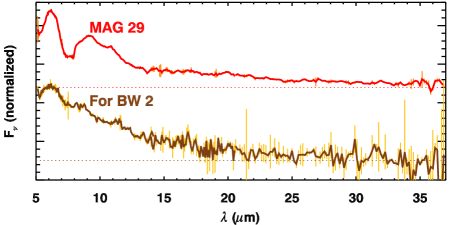
Figure 5.— The full IRS spectra for MAG 29 and For BW 2, which were observed in both SL and LL. The dotted lines mark the zero-flux levels for both spectra.

Figures 2–4 present the final SL spectra for our 19 targets. Figure 5 presents the full spectra for the two sources also observed in LL.

4. Refining the metallicity estimates

4.1. Bolometric magnitudes

Table 7Bolometric magnitudes

Source	Our	External	Other values for $M_{\rm bol}$
name	$M_{\rm bol}$	uncertainty	M07	L08	G09	SAAO
MAG 29	$-$4.90 $\pm$ 0.04	$\cdots$	$\cdots$	$\cdots$	$\cdots$	$\cdots$
Scl V78 V544	$-$4.20 $\pm$ 0.04	$\cdots$	$\cdots$	$\cdots$	$\cdots$	$\cdots$
For BW 2	$-$4.41 $\pm$ 0.29	0.25	$\cdots$	$\cdots$	$-$4.05	$\cdots$
For BTH 13-23	$-$4.28 $\pm$ 0.04	0.30	$-$4.90	$-$4.84	$\cdots$	$-$4.45
For BTH 12-4	$-$4.90 $\pm$ 0.04	0.29	$-$5.52	$-$5.26	$-$5.20	$-$4.80
For BTH 3-129	$-$4.65 $\pm$ 0.04	0.17	$-$4.95	$\cdots$	$\cdots$	$-$4.68
For DK 18	$-$4.88 $\pm$ 0.04	0.54	$\cdots$	$\cdots$	$-$4.11	$\cdots$
For DK 52	$-$4.62 $\pm$ 0.04	0.02	$\cdots$	$\cdots$	$-$4.65	$\cdots$
For DI 2	$-$4.06 $\pm$ 0.29	0.34	$\cdots$	$\cdots$	$-$3.58	$\cdots$
For WEL C10	$-$4.61 $\pm$ 0.04	0.20	$-$4.60:	$\cdots$	$\cdots$	$-$4.21
For BW 69	$-$3.98 $\pm$ 0.04	0.06	$\cdots$	$\cdots$	$-$4.07	$\cdots$
For BW 75	$-$4.35 $\pm$ 0.04	0.22	$-$4.67	$\cdots$	$-$4.25	$\cdots$
For BW 83	$-$4.57 $\pm$ 0.04	0.19	$\cdots$	$\cdots$	$-$4.61	$-$4.27
ALW Car 2	$-$4.54 $\pm$ 0.29	$\cdots$	$\cdots$	$\cdots$	$\cdots$	$\cdots$
Car MCA C3	$-$4.82 $\pm$ 0.29	$\cdots$	$\cdots$	$\cdots$	$\cdots$	$\cdots$
Car MCA C5	$-$4.57 $\pm$ 0.29	$\cdots$	$\cdots$	$\cdots$	$\cdots$	$\cdots$
Leo I MFT C	$-$4.77 $\pm$ 0.13	0.47	$\cdots$	$\cdots$	$\cdots$	$-$5.44
Leo I MFT A	$-$4.43 $\pm$ 0.13	0.23	$\cdots$	$\cdots$	$\cdots$	$-$4.75
Leo I MFT E	$-$4.34 $\pm$ 0.13	0.42	$\cdots$	$\cdots$	$\cdots$	$-$3.74

We estimate bolometric magnitudes by integrating the IRS spectra, combined with the available optical and NIR photometry. Table 7 presents the results and compares them with previously published estimates. Over the region covered by the spectrum, simple integration suffices. Below 5.1 $\mu$m, we integrate on a grid of $F_{\lambda}$ vs. wavelength linearly interpolated through the photometry in Tables 4 and 5. We extrapolate with a Rayleigh-Jeans tail at the long-wavelength end and a Wien distribution at the short-wavelength end. The final magnitudes are scaled to the distances given in Table 1.

This paper marks a shift from previous determinations of bolometric magnitude. Before, we did not consider $BVRI$ photometry. The change is significant. The Wien distribution extrapolated from $J$ overestimates the flux in the visual regime by $\sim$0.2 magnitudes for our bluest sources, because the combination of molecular band absorption and dust extinction drops more quickly with decreasing wavelength. The largest difference in our sample is 0.27 magnitudes. The difference decreases to zero past $J-K\sim 3$. A line can be fitted to this shift: $\Delta M_{\rm bol}=0.27-0.075(J-K)$, although the scatter is $\sim$0.1 magnitudes. It would be appropriate to apply this correction to our previously published bolometric magnitudes for carbon stars (e.g., Sloan et al., 2006, and most of the other IRS papers cited in §1).

We have simplified the treatment of the $BVRI$ photometry by not considering differences in photometric systems or attempting transformations among them. Such an effort would have virtually no impact on the bolometric magnitudes reported here. However, for the NIR photometry, we did distinguish between the SAAO and 2MASS systems, as it is in this wavelength regime that the spectral energy distributions (SEDs) of our sources peak.

The impact of the correction for interstellar reddening is much smaller. It brightens the bluest stars by only $\sim$0.02 magnitudes in our samples, with the correction decreasing to nearly zero for the most enshrouded carbon stars. The redder the $J-K$ color, the more the peak of the SED has shifted away from wavelengths most affected by interstellar reddening.

The most significant source of uncertainty in our sample is the variability of the star. The $JHK$ photometry dominates the final bolometric magnitude. Comparing the mean magnitudes from the SAAO to the 2MASS data reveals an average difference ($|\Delta M_{\rm bol}|$) of 0.29 magnitudes, in either direction, with differences as large as 0.6 magnitudes. Interestingly, we get similarly large differences if we only consider the sources identified as semi-regulars, irregulars, or simply “variables”. For any variable star, the mean magnitude is definitely preferable to NIR photometry that only sparsely covers the period of variability.

For the sources with mean NIR magnitudes, the uncertainties in bolometric magnitude in Table 7 are just the uncertainty in distance modulus. For the remaining five sources, we set the uncertainties to 0.29 to reflect the limitations of the 2MASS photometry. The reader should bear in mind, though, that errors as large as 0.6 magnitudes are possible.

Table 7 also lists what we describe as “external” uncertainties in $M_{\rm bol}$. These are the standard deviation of all values of $M_{\rm bol}$ for a given star in Table 7. The values from other authors have been adjusted to our adopted distance moduli (in Table 1). The values published by Matsuura et al. (2007) are based on earlier versions of the IRS data for the five stars in common between this work and theirs. They used these data along with the NIR photometry from the SAAO and fitted radiative transfer models to determine the luminosity. Four of their bolometric magnitudes appear in their Table 4; we reconstructed the fifth from the luminosity given in the text. Lagadec et al. (2008) used 2MASS photometry and applied the bolometric corrections defined by Whitelock et al. (2006), which were calibrated from Galactic carbon stars with photometry from the optical into the mid-infrared, including mean magnitudes at $JHK$, IRAS data to 25 $\mu$m and MSX data to 15 $\mu$m. Groenewegen et al. (2009a) applied the bolometric corrections defined by Bessell & Wood (1984) to 2MASS photometry. The bolometric magnitudes from the SAAO in Table 7 are based on mean magnitudes at $JHK$ and the bolometric corrections of Whitelock et al. (2006). The external uncertainties may well overestimate our actual uncertainty in $M_{\rm bol}$ as they reflect systematic differences between groups with access to different data, but including these systematics will force us to be cautious with our $M_{\rm bol}$ results.

4.2. Masses and metallicities

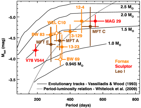
Figure 6.— The 11 sources for which we have periods plotted on a period-luminosity (P-L) diagram and compared to evolutionary tracks by Vassiliadis & Wood (1993) and the P-L relation of Whitelock et al. (2009). The masses given are initial values in solar masses. For $M_{\rm bol}$, the error bars are the larger of the uncertainties in Table 7, with a minimum assumed uncertainty of 0.15 magnitudes (which affects Fornax BW 69 and the two Sculptor objects). We have assumed a 10% uncertainty in period. To avoid clutter in the figure, we have shortened the source names. The two open circles mark the semi-regular variables.

Table 8Possible stellar ages

Source	Estimated	Estimated
name	initial mass ($M_{\odot}$)	age (Gyr)
MAG 29	1.5–1.9	0.9–1.7
Scl V78 V544	1.2–1.8	1.0–3.5
For BTH 13-23	0.97–1.5	1.8–11
For BTH 12-4	1.4–2.2	0.6–2.7
For BTH 3-129	1.3–1.7	1.2–3.3
For WEL C10	1.3–1.9	0.9–3.3
For BW 69	0.94–1.1	5.5–12
For BW 83	1.3–2.0	0.8–3.3
Leo I MFT C	1.0–2.3	0.5–6.9
Leo I MFT A	1.0–1.5	1.7–6.9
Leo I MFT E	0.98–1.9	0.8–7.3

We have pulsation periods for 11 of our 19 targets, including both carbon stars in Sculptor, all three in Leo I, and six of the 11 in Fornax (see Table 5). Figure 6 compares their periods and bolometric magnitudes to evolutionary tracks by Vassiliadis & Wood (1993), allowing us to make rough estimates of their initial mass, and thus their age. The evolutionary tracks convert the relatively robust period-mass-radius relation from stellar pulsation theory into a period-mass-luminosity relation by assuming a relation between effective temperature and luminosity. The mass-loss history must be estimated to convert current to initial mass, and the histories utilized by Vassiliadis & Wood (1993) have successfully reproduced the luminosities at the tips of the RGB in Magellanic clusters. More theoretical approaches to the problem (e.g., Kamath et al., 2011) basically validate the older evolutionary tracks.

The error bars in Figure 6 are the larger of the internal and external uncertainties for $M_{\rm bol}$ in Table 7, although we have assumed a minimum uncertainty of 0.15 magnitudes, which affects MAG 29 and V78 V544 in Sculptor and For BW 69. For period, we assumed a 10% uncertainty, based on the fact that Groenewegen et al. (2009b) have found shifts in period on this order for some of the sources in their sample (not counting those sources with possible changes in pulsation mode). Our conservative approach to the uncertainties leads to a fairly wide range of initial masses and ages in our sample, but even these broad limits can help constrain the metallicities.

Table 8 gives our rough estimates of initial masses and current ages, based on Figure 6. Assuming that the stellar lifetimes scale as $M^{-2.5}$ would overestimate the ages, because more metal-poor stars evolve off of the main sequence more quickly. To estimate the ages, we have used models by Maraston (2005), who give main-sequence turn-off masses at metallicities of [Fe/H] = $-$1.35, $-$0.33, and 0.0. The first metallicity matches Leo I perfectly. For Sculptor we spline interpolated to [Fe/H] = $-$1.0. For Fornax, we spline interpolated to $-$0.3 and $-$0.8, using the former for the lower bound on the mass and the latter for the upper bound. To get from main-sequence turn-off point to the AGB, we assumed that a star spends a time on the red giant branch equal to 10% of its main-sequence lifetime.

The likely ages of both stars in Sculptor are consistent with the models of Revaz et al. (2009), which show virtually no star formation in Sculptor over the period from $\sim$8 to $\sim$2 Gyr ago. Thus both stars must be younger than $\sim$2 Gyr old. Their models indicate that stars produced in this recent round of star formation have [Fe/H] $\sim$ $-$1.0. This value is significantly higher than the mean in Table 1 and the value of $-$1.4 assumed by Sloan et al. (2009).

Menzies et al. (2011) also placed MAG 29 in the younger population in Sculptor, with an age of $\sim$1–2 Gyr. However, they made this estimate based on its pulsation period, which they argue is a good diagnostic for age (see their § 6 and references therein. They assigned Scl V78 V544 in the older population due to its shorter pulsation period, while we find that its luminosity is more consistent with the younger population (age $\lesssim$ 2 Gyr). The discrepancy between the two approaches arises from the significant spread in periods possible for stars of a given mass.

Two of the targets in Fornax, WEL C10 and BW 69, are semi-regular pulsators. The location of For BW 69 amongst the other data suggests that it is a fundamental-mode pulsator. If it were pulsating in the first overtone, then its position in Figure 6 would correspond to a period $\sim$2.2 times longer (Wood & Sebo, 1996), which would imply an unreasonably low mass. If For WEL C10 were pulsating in the first overtone, it would shift to the right-most point in the figure and become something of an outlier. While we suspect that it is pulsating in the fundamental mode, an error here would have only a small impact on its estimated mass, because the track for 1.5 M_⊙ is nearly horizontal.

Four of the six sources with periods in Fornax have relatively young ages of $\sim$3.3 Gyr or less. The models of Revaz et al. (2009) suggest stars of this age would have corresponding metallicities in the range $-$0.8 $<$ [Fe/H] $<$ $-$0.3. This range is fairly constant over the likely time frame, and it is more similar to the Magellanic samples than to the other dwarf spheroidals considered here. The uncertain mass of BTH 13-23 leads to an unconstrained age and a poorly constrained metallicity. BW 69 looks to be at least 5.5 Gyr old. Using the models of Revaz et al. (2009) as a guide, its maximum metallicity is $\sim$$-$0.5, the mean metallicity of the SMC, although it cold be more metal-poor.

Five stars in Fornax without periods do not appear in Figure 6. Two were outside the survey area of Whitelock et al. (2009), and both were identified as variables by other observers (see Table 5). Whitelock et al. (2009) identified the other three as variables but were unable to report a period. All five bolometric magnitudes do little to constrain their likely masses, ages, and metallicities, which we will assume are similar to the sources for which we have periods.

The three carbon stars in Leo I are probably younger than $\sim$7 M_⊙, but their relatively unconstrained masses allow us to say little more about their age. Fortunately for our efforts to constrain their metallicity, the MDF for Leo I is narrow ($<$[Fe/H]$>$ = $-$1.35 $\pm$ 0.24, see § 2.2). No matter their mass and age, these stars are likely to be more metal-poor than those in Fornax and even Sculptor.

The SAAO reports that all three of our targets in Carina are semi-regular variables, but the periods are undetermined (J. Menzies, P. Whitelock, and M. W. Feast, 2011, private communication). As with Leo I, the metallicities in Carina are distributed more narrowly than in Sculptor or Fornax: $<$[Fe/H]$>$ = $-$1.73 $\pm$ 0.35, making it likely that these targets are even more metal-poor than those in Leo I. The metallicity measurement by Abia et al. (2008) reinforces this point; they found [M/H] = $-$1.7 for MCA C3.

Thus the metallicities of the carbon stars observed in Fornax and Sculptor are probably higher than previously proposed. While Matsuura et al. (2007) adopted [Fe/H] $\sim$ $-$1.0 for the five Fornax stars they examined, we find that [Fe/H] appears to be more Magellanic in nature: $\sim$$-$0.3 to $-$0.8. Similarly, while Sloan et al. (2009) suggested that MAG 29, which is also associated with significant quantities of carbon-rich dust, would have formed with [Fe/H] $\sim$ $-$1.4, we have revised this metallicity up to $\sim$$-$1.0.

Figure 6 includes the P-L relation of Whitelock et al. (2009): $M_{\rm bol}$ = $-$3.3 log $P$ (days) + 3.979. This relation appears on the plot as a narrow dotted curve, but for typical data, it is $\sim$0.4–0.5 magnitudes wide at any period. Most of our data fall within this range. The evolutionary tracks show why a significant spread in periods would be expected for stars of a given mass (and therefore age). For stars of mass $\gtrsim$ 1.5 M_⊙, once they reach pulsation periods of $\sim$350–400 days, their period will continue to increase, but their luminosity will remain largely fixed. Thus the width of the P-L relation depends on how long AGB stars will survive once they begin pulsating in the fundamental mode. This width can lead to considerable uncertainty in any distances determined using P-L relations for LPVs, and for this reason we did not include distances based on the periods of LPVs in § 2.1 above.

4.3. Comparison samples

In the analysis below, we compare the carbon stars we have observed in the four targeted dwarf spheroidal galaxies with similar infrared spectroscopy of samples in the Milky Way, LMC, and SMC. The Galactic spectra are from the atlas of spectra from the Short-Wavelength Spectrometer (SWS) on the Infrared Space Observatory (ISO) (Sloan et al., 2003). The sample includes the 37 sources classified by Kraemer et al. (2002) as carbon stars, including nine stars observed multiple times. Using the multiple observations, we have arrived at typical variations over the pulsation cycle of the star in the strengths of the extracted features; these are plotted in the relevant figures to give an idea of the systematic uncertainties in the data. See the description by Sloan et al. (2006) for more detail on the Galactic sample. A paper in preparation will present the spectral properties of this sample in more detail.

The Magellanic samples of carbon stars come from the following programs: 200, 1094, 3277, 3426, 3505, and 3591. The publications arising from these programs are referenced in §1. These samples include a total of 72 carbon stars in the LMC and 34 in the SMC.

Some caution is required when comparing spectral data amongst the samples, as a variety of selection criteria bias them in different ways. For example, Programs 1094 and 3591 focused on dusty sources in the LMC, thus selecting against optically thin dust shells, while Program 3426 sampled the brightest infrared sources in the LMC, which again selected against optically thin dust shells. The impact of these particular criteria is readily apparent in the following figures. For this reason, we will attempt to compare the data in the different samples by plotting the variable of interest against a dependent variable. The effect of metallicity will reveal itself through changes in the dependency from one galaxy to the next.

5. Spectral analysis

5.1. The Manchester Method

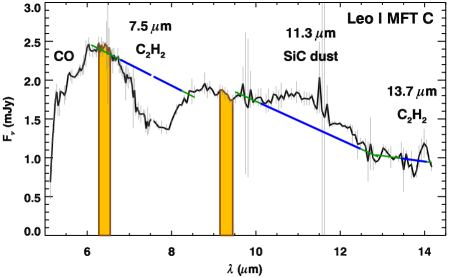
Figure 7.— An example of the carbon-rich dust and molecular features in the spectrum of Leo I MFT C. We use the Manchester Method to measure the [6.4]$-$[9.3] color, the strength of the SiC dust emission feature at 11.3 $\mu$m (or other dust features in the vicinity), and the acetylene absorption bands at 7.5 and 13.7 $\mu$m. Note that the latter is just the Q branch of a much broader feature. The method estimates the strength of the SiC and C₂H₂ features line segments, with the continua estimated over the ranges where the lines are thin and the features measured where the lines are thick. Table 10 gives the [6.4]$-$[9.3] colors and SiC feature strengths, while Table 11 gives the equivalent widths for the acetylene bands.

Table 9Fitting wavelengths

Feature	$\lambda$	Blue continuum	Red continuum
	($\mu$m)	($\mu$m)	($\mu$m)
C2H2 abs.	7.5	6.08–6.77	8.25–8.55
SiC dust em.	11.3	9.50–10.10	12.50–12.90
C2H2 abs.	13.7	12.80–13.40	14.10–14.70

Table 10Spectral dust properties

Source	[6.4.]$-$[9.3]	Mass-loss rates (M⊙/yr)		“SiC” feature strength
name	(mags.)	total ($\log\dot{M}$)	dust ($\log\dot{D}$)	$\lambda_{c}$ ($\mu$m)	feature/continuum
MAG 29	0.432 $\pm$ 0.008	$-$5.91	$-$8.21	10.87 $\pm$ 0.08	0.028 $\pm$ 0.005
Scl V78 V544	$-$0.147 $\pm$ 0.016	$\cdots$	$\cdots$	$\cdots$	0.061 $\pm$ 0.034
For BW 2	0.333 $\pm$ 0.015	$-$6.07	$-$8.37	11.51 $\pm$ 0.16	0.084 $\pm$ 0.013
For BTH 13-23	0.716 $\pm$ 0.006	$-$5.45	$-$7.75	11.29 $\pm$ 0.07	0.133 $\pm$ 0.006
For BTH 12-4	0.602 $\pm$ 0.005	$-$5.64	$-$7.94	11.27 $\pm$ 0.12	0.045 $\pm$ 0.004
For BTH 3-129	0.592 $\pm$ 0.006	$-$5.65	$-$7.95	11.23 $\pm$ 0.04	0.173 $\pm$ 0.005
For DK 18	0.152 $\pm$ 0.021	$-$6.36	$-$8.66	11.48 $\pm$ 0.28	0.120 $\pm$ 0.024
For DK 52	0.198 $\pm$ 0.031	$-$6.28	$-$8.58	11.50 $\pm$ 0.43	0.093 $\pm$ 0.031
For DI 2	$-$0.153 $\pm$ 0.068	$\cdots$	$\cdots$	11.34 $\pm$ 0.15	0.317 $\pm$ 0.053
For WEL C10	$-$0.046 $\pm$ 0.022	$\cdots$	$\cdots$	11.80 $\pm$ 0.33	0.051 $\pm$ 0.015
For BW 69	0.232 $\pm$ 0.023	$-$6.23	$-$8.53	$\cdots$	0.011 $\pm$ 0.026
For BW 75	0.156 $\pm$ 0.019	$-$6.35	$-$8.65	$\cdots$	0.032 $\pm$ 0.018
For BW 83	0.163 $\pm$ 0.032	$-$6.34	$-$8.64	11.93 $\pm$ 0.26	0.041 $\pm$ 0.014
ALW Car 2	$-$0.025 $\pm$ 0.028	$\cdots$	$\cdots$	$\cdots$	0.012 $\pm$ 0.047
Car MCA C3	$-$0.157 $\pm$ 0.018	$\cdots$	$\cdots$	$\cdots$	$-$0.008 $\pm$ 0.039
Car MCA C5	$-$0.031 $\pm$ 0.031	$\cdots$	$\cdots$	$\cdots$	0.088 $\pm$ 0.056
Leo I MFT C	0.500 $\pm$ 0.015	$-$5.80	$-$8.10	11.24 $\pm$ 0.45	0.155 $\pm$ 0.043
Leo I MFT A	0.069 $\pm$ 0.016	$-$6.49	$-$8.79	$\cdots$	0.080 $\pm$ 0.038
Leo I MFT E	0.226 $\pm$ 0.012	$-$6.24	$-$8.54	11.32 $\pm$ 0.22	0.196 $\pm$ 0.026

Table 11Spectral acetylene properties

Source	7.5 $\mu$m C2H2 band		13.7 $\mu$m C2H2 band (Q branch)
name	$\lambda_{c}$ ($\mu$m)	EW ($\mu$m)	$\lambda_{c}$ ($\mu$m)	EW ($\mu$m)
MAG 29	7.49 $\pm$ 0.02	0.780 $\pm$ 0.012	13.69 $\pm$ 0.04	0.079 $\pm$ 0.007
Scl V78 V544	7.31 $\pm$ 0.15	0.186 $\pm$ 0.013	$\cdots$	0.144 $\pm$ 0.031
For BW 2	7.34 $\pm$ 0.09	0.112 $\pm$ 0.010	$\cdots$	$-$0.002 $\pm$ 0.029
For BTH 13-23	7.43 $\pm$ 0.02	0.238 $\pm$ 0.004	13.68 $\pm$ 0.03	0.042 $\pm$ 0.004
For BTH 12-4	7.52 $\pm$ 0.08	0.050 $\pm$ 0.004	13.70 $\pm$ 0.02	0.058 $\pm$ 0.003
For BTH 3-129	7.42 $\pm$ 0.02	0.191 $\pm$ 0.005	13.66 $\pm$ 0.02	0.030 $\pm$ 0.002
For DK 18	7.46 $\pm$ 0.11	0.160 $\pm$ 0.011	$\cdots$	0.040 $\pm$ 0.032
For DK 52	$\cdots$	0.117 $\pm$ 0.024	13.80 $\pm$ 0.08	0.157 $\pm$ 0.027
For DI 2	7.24 $\pm$ 0.13	0.183 $\pm$ 0.035	$\cdots$	0.122 $\pm$ 0.051
For WEL C10	7.47 $\pm$ 0.05	0.178 $\pm$ 0.008	$\cdots$	0.095 $\pm$ 0.013
For BW 69	7.44 $\pm$ 0.15	0.149 $\pm$ 0.021	$\cdots$	0.034 $\pm$ 0.021
For BW 75	7.52 $\pm$ 0.11	0.136 $\pm$ 0.009	$\cdots$	0.019 $\pm$ 0.021
For BW 83	7.48 $\pm$ 0.16	0.146 $\pm$ 0.020	13.66 $\pm$ 0.09	0.130 $\pm$ 0.023
ALW Car 2	$\cdots$	$-$0.074 $\pm$ 0.023	$\cdots$	$-$0.341 $\pm$ 0.034
Car MCA C3	$\cdots$	0.040 $\pm$ 0.014	13.70 $\pm$ 0.09	0.150 $\pm$ 0.020
Car MCA C5	$\cdots$	$-$0.018 $\pm$ 0.018	$\cdots$	0.127 $\pm$ 0.028
Leo I MFT C	7.52 $\pm$ 0.05	0.315 $\pm$ 0.010	$\cdots$	$-$0.008 $\pm$ 0.020
Leo I MFT A	7.43 $\pm$ 0.08	0.251 $\pm$ 0.016	$\cdots$	0.083 $\pm$ 0.036
Leo I MFT E	7.53 $\pm$ 0.14	0.075 $\pm$ 0.013	$\cdots$	0.039 $\pm$ 0.019

The mid-infrared spectra of carbon stars are rich in emission and absorption features. Figure 7 illustrates how we sort these out for one spectrum, using the Manchester Method, which was first developed for IRS spectra of carbon stars in the Magellanic Clouds (Sloan et al., 2006; Zijlstra et al., 2006). The [6.4]$-$[9.3] color samples the spectra at 6.25–6.55 and 9.10–9.50 $\mu$m. These two wavelength intervals are relatively free of emission or absorption features, and as detailed in § 5.2 below, can be used to estimate the total amount of dust emission in the spectrum. For ease of reference, we will refer to this quantity as “dust content” in the following discussion. To measure the relative strengths of the acetylene bands and SiC emission features in the spectra, we use line segments to estimate the continuum above or below the feature. Table 9 gives the wavelengths used to fit continua and measure the various features. For the molecular bands, we report an equivalent width (EW); for the SiC dust emission, we report its total integrated strength, divided by the continuum underneath, as estimated by the fitted line segment. For all features, we also report a central wavelength, defined as the wavelength which bisects the integrated flux of the feature. The uncertainty in the central wavelength indicates the range possible given the uncertainty in the extracted strength.

Table 10 presents the [6.4]$-$[9.3] color and the relative strength of the SiC dust emission feature at $\sim$11.3 $\mu$m. The SiC feature is covered below in § 5.3. Table 11 presents the equivalent widths and central wavelengths of the absorption bands from acetylene gas, as described in § 5.4.

5.2. Dust content and pulsation period

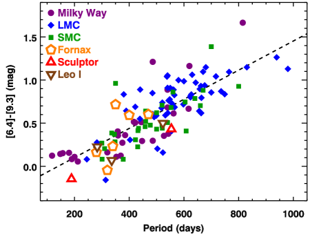
Figure 8.— The relation between [6.4]$-$[9.3] color and pulsation period for our sample of carbon stars in Local Group dwarfs, compared to samples from the Galaxy, LMC, and SMC. The uncertainties in [6.4]$-$[9.3] color are generally smaller than the plotting symbols, and it is reasonable to assume that the uncertainty in period is about 10%. The dashed curve is a line fitted to all of the stars with periods in the Milky Way, LMC, SMC, and Fornax. All four galaxies show a similar dependence of total dust content on pulsation period, despite their differences in metallicity. However, all five stars in Sculptor and Leo I lie below the line at a statistically significant level, indicating that the impact of metallicity is revealing itself for the most metal-poor stars sampled.

The [6.4]$-$[9.3] color measures the total emission from the star plus shell in two wavelength ranges between the various absorption and emission features. Amorphous carbon, which dominates the dust around carbon stars (see Martin & Rogers, 1987), has no resonances in the infrared, so that the apparent “continuum” in a spectrum is actually a combination of star plus dust. The [6.4]$-$[9.3] color provides a means of measuring the relative combinations of these two components and thus serves as a proxy for total dust content.

Groenewegen et al. (2007, their Fig. 7) calibrated the [6.4]$-$[9.3] color to total mass-loss rate by applying radiative transfer models to a large sample of IRS spectra of Magellanic carbon stars. They found a linear relationship between the log of the total mass-loss rate and the [6.4]$-$[9.3] color. Because their models used the same gas-to-dust ratio ($\psi$ = 200) and the same outflow velocity ($v_{\rm out}$ = 10 km/s) for all stars, their calibration of the [6.4]$-$[9.3] color actually ties it directly to the total mass of warm dust contributing in the 6–10 $\mu$m spectral region. Dividing $\dot{M}$ by the gas-to-dust ratio gives the dust production rate ($\dot{D}$, DPR, or dust MLR), and dividing $\dot{D}$ by the outflow velocity gives a quantity proportional to the optical depth of the radiating dust, which we are calling the dust content.

Sloan et al. (2008) presented the dust-color relation in terms of log $\dot{D}$ vs. [6.4]$-$[9.3]. Adding a term to account for the outflow velocity and correcting their typographical error,

$$\log~{}\dot{D}\left(\frac{{\rm M_{\odot}}}{{\rm yr}}\right)=\log\,\left(\frac{v_{{\rm out}}}{10\,{\rm km/s}}\right)$$

$$\times\,\{~{}-8.9+1.6\,([6.4]-[9.3])~{}\}.$$ (1)

This equation makes no assumptions about outflow velocity, and it is free of any dependence on gas-to-dust ratio. We will return to the question of how these quantities vary with metallicity in § 6.5 below.

Table 10 gives the [6.4]$-$[9.3] color for each source. In order to translate these colors into more familiar quantities, Table 10 also provides $\dot{D}$ using the above equation and an assumed outflow velocity of 10 km/s and $\dot{M}$ assuming $\psi$ = 200. It is important to remember, though, that the [6.4]$-$[9.3] color actually measures the dust content.

Sloan et al. (2008) compared the dust content in carbon stars in Magellanic and Galactic samples by plotting the [6.4]$-$[9.3] color as a function of the pulsation period of the star (their Fig. 29). They found that the amount of dust as measured by the [6.4]$-$[9.3] color increases with pulsation period. The scatter in [6.4]$-$[9.3] color at a given period is substantial. Within this envelope, no dependency on metallicity was apparent between the samples from the Galaxy, LMC or SMC.

Earlier publications of data from our Local Group sample did not have the benefit of the periods determined from the SAAO, but we are now in a position to compare our Local Group carbon stars directly to the other samples. Figure 8 includes data for carbon stars in Fornax, Sculptor, and Leo I, along with the comparison sample from the Galaxy, LMC, and SMC. The overall dependency of dust content with pulsation period is unchanged. The new Fornax data appear to follow the same dependency, although the period coverage is smaller. This similarity is consistent with our revised metallicity. The figure includes a line fitted to all of the Galactic, Magellanic, and Fornax data:

$$[6.4]-[9.3]=-0.227+0.00169\,\,P\,{\rm(days)}.$$ (2)

Interestingly, the five spectra from Sculptor and Leo I all lie below the fitted line in Figure 8. The mean difference for these five is $-$0.185 magnitudes, with an uncertainty in the mean of 0.047 magnitudes. The comparison data, including Fornax, show a standard deviation of 0.209 magnitudes about the fitted line, and with a sample of 121 objects with periods, the uncertainty in the mean is 0.019 magnitudes. Adding the uncertainties in quadrature gives an uncertainty in the difference between the fitted line and the data from Sculptor and Leo I of 0.051 magnitudes, making the difference between them and the other samples 3.6 $\sigma$.

In contrast, the mean difference between the Fornax data and the fitted line in Figure 8 is only 0.018 magnitudes. Comparing this difference to a standard deviation of 0.241 and an uncertainty in the mean of 0.098 magnitudes shows that Fornax follows the Magellanic and Galactic samples.

The difference for Sculptor and Leo I is statistically significant. The carbon stars in these two galaxies almost certainly do not belong to the same population as Fornax, the SMC, the LMC, and the Galaxy ($p$ value = 0.00014). Nonetheless, we have only five deviant spectra, further verification with larger samples would be helpful. While we have revised previous estimates of the metallicity of the carbon stars in Fornax upward to Magellanic values and the metallicity in Sculptor from $-$1.4 to $-$1.0, the Leo I sample restores the range of [Fe/H] sampled in this analysis down to $\sim$ $-$1.35. We conclude that for the most metal-poor stars in our sample, the impact of the initial metallicity of the star on its future dust production as a carbon-rich AGB star is large enough to be noticeable in the infrared.

5.3. Silicon carbide dust emission

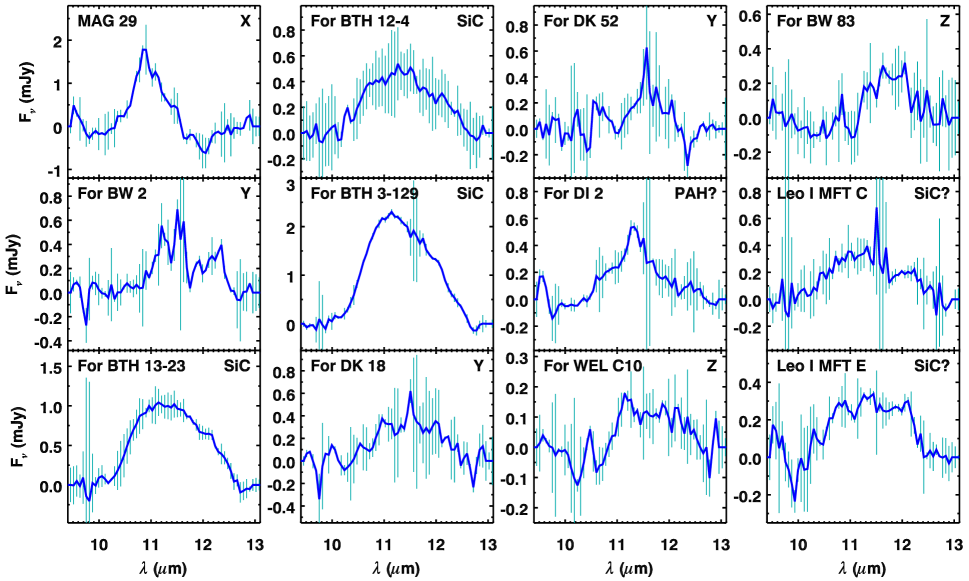
Figure 9.— The extracted spectral features in the vicinity of the SiC dust emission feature for the 12 spectra where the extracted flux has a S/N ratio $>$ 2.5, along with identifications of the features where possible. “X” refers to the apparent feature in the spectrum of MAG 29 centered at 10.9 $\mu$m and most likely due to the continuum between molecular absorption bands. “Y” labels features with a central wavelength at $\sim$11.5 $\mu$m, and “Z” labels features centered to the red, $\sim$11.8–11.9 $\mu$m.

5.3.1 In the dwarf spheroidals

The SiC feature at $\sim$11.3 $\mu$m is generally weak in this sample. Only three sources show an unambiguous SiC feature, although two more have spectral structure consistent with it. In Table 10, seven features have a S/N ratio $<$ 2.5. For these, the central wavelength is omitted because it is meaningless; their continuum-subtracted spectra are essentially noise in this region. Figure 9 illustrates the extracted features in the vicinity of 11.3–11.5 $\mu$m for the remaining 12 sources which have an extracted strength with a S/N ratio $>$ 2.5.

The five probable or possible SiC features all have central wavelengths of 11.2–11.3 $\mu$m. Three of these are in Fornax (BTH 3-129, 12-4, and 13-23), and they were all discussed previously by Matsuura et al. (2007). The other two are in Leo I. In both cases, the emission profile is not a perfect match for SiC, but given the noise, SiC is the most likely explanation.

Fornax DI 2 has an emission feature which peaks at 11.3 $\mu$m and has a width and shape consistent with the out-of-plane C–H solo bending mode in polycyclic aromatic hydrocarbons (PAHs). The problem with this assignment is that no other PAH features can be identified with any confidence. There is a hint of the 8.6 $\mu$m feature, but noise masks the 6.2 $\mu$m feature, and acetylene absorption would hide the 7.5–7.9 $\mu$m emission complex. No 12.7 $\mu$m feature is apparent.

Other features in Figure 9 can be placed in three groups, labelled “X”, “Y”, and “Z”.

MAG 29 has the sole “X” feature, an apparent emission feature centered at 10.9 $\mu$m, but its strength amounts to only 3% of the continuum integrated over the same wavelength range. Given the strong molecular absorption bands in this spectrum (§ 5.4), we suspect that the apparent peak at $\sim$11 $\mu$m is simply the continuum between molecular absorption bands. C₃ at 10 $\mu$m might explain the drop to the blue side of this “feature” (Zijlstra et al., 2006). The drop to the red could be due to the broad wings of the C₂H₂ band centered at 13.7 $\mu$m, which grow wider for higher gas temperatures.

Three spectra show what we are calling the “Y” feature, which peaks at $\sim$11.5 $\mu$m and is sharper and more symmetric than the SiC feature. These features are weak, and the spectra have poor S/N ratios, preventing any conclusive statements about their carrier. Nonetheless, it should be noted that graphite produces an emission feature in this spectral range (Draine & Lee, 1984; Laor & Draine, 1993). The absence of this feature in the spectrum of IRC +10216 (Martin & Rogers, 1987) and other Galactic carbon stars led to the currently favored model where amorphous carbon, and not graphite, dominates the dust around carbon stars. The 11.5 $\mu$m graphite feature arises from C–C displacements between graphene sheets, and in laboratory data it is exceptionally narrow due to the regular spacing and large extent of these sheets. Smaller sheets and irregularities in the lattice structure would fatten the feature, but whether or not it would have a shape like the observed “Y” feature is unknown. The presence of graphite in carbon-rich dust shells is an interesting possibility, but given the limited quality of the extracted features, any further speculation is unwarranted.

Two spectra show possible emission features in this range which peak further to the red, in the 11.8–11.9 $\mu$m region. We are calling this the “Z” feature. As with the “Y” feature, though, the data are noisy. One could argue that the feature in the spectrum of For WEL C10 is a very noisy example of SiC emission, while the feature in For BW 63 could be a noisy “Y” feature.

5.3.2 Comparing the samples

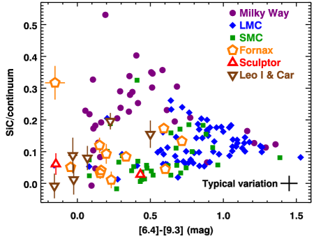
Figure 10.— The strength of the SiC dust emission at $\sim$11.3 $\mu$m, relative to the underlying continuum from star and amorphous carbon dust, plotted as a function of [6.4]$-$[9.3] color. The error bars labelled “Typical variation” indicate the expected changes in spectral properties over a pulsation cycle of the central star. The uncertainties are plotted for the program stars, but they are generally smaller than the plotting symbols. The Galactic carbon stars follow a different sequence than most of the carbon stars in the other galaxies. The one data point from Fornax with [6.4]$-$[9.3] = $-$0.15 and SiC/cont. = 0.32 is For DI 2, which appears to show emission from PAHs and not SiC at $\sim$11.3 $\mu$m.

Figure 10 plots the strength of the SiC dust emission, normalized to the underlying continuum as a function of the [6.4]$-$[9.3] color. The SiC dust strength is integrated between 10.1 and 12.5 $\mu$m and divided by the total “continuum” emission in the same interval, where “continuum” is the combination of emission from amorphous carbon dust and the central star.

Sloan et al. (2006) found that the relative strength of the SiC emission feature decreased as the metallicity of the sample decreased. In Figure 10, two different sequences of relative SiC strength vs. total dust content are apparent, with a clear bimodality at colors of $\sim$0.2–0.6. In this range, Galactic stars dominate the upper sequence, with not one falling on the lower sequence. Once [6.4]$-$[9.3] exceeds $\sim$0.6, the sequences begin to merge, although the difference between the Galactic and Magellanic samples is still evident.

Generally, the carbon stars in the dwarf spheroidals follow the lower sequence in Figure 10. Fornax DI 2 (with [6.4]$-$[9.3] = $-$0.15 and SiC/cont. = 0.32) is the most significant exception, showing an emission feature at 11.3 $\mu$m with strong contrast to the continuum but virtually no other dust. This emission feature looks more like PAHs than SiC (see Figure 9), but as discussed above, that identification is problematic and uncertain. The blue [6.4]$-$[9.3] color indicates that For DI 2 is virtually naked, making SiC dust unlikely. Another major exception is Leo I MFT E ([6.4]$-$[9.3] = 0.23, SiC/cont. = 0.20). In this case, the feature is most likely SiC and the exception appears to be real.

Three carbon stars in dwarf spheroidals appear in Figure 10 with SiC/cont. $>$ 0.13 and [6.4]$-$[9.3] $>$ 0.45. These objects are (left to right in Figure 10): Leo I MFT C, For BTH 3-129, and For BTH 13-23. While the apparent SiC emission in Leo I MFT C is somewhat noisy, its profile is consistent with SiC. The identifications of the features in the two Fornax spectra are firm, due to the strength and profiles of these features. We see no obvious characteristics to distinguish these sources from the others with weaker SiC features, much as Sloan et al. (2006) found when investigating the five SMC sources in the same region. None of these eight stand out in terms of pulsation period, luminosity, or any other identified property. Why they have stronger SiC features than other sources from the same galaxies remains unknown.

The sources in Fornax show SiC strengths similar to the Magellanic sources, fully consistent with the metallicities we believe they formed with. The general lack of dust in the three Carina sources places them in the lower left corner of Figure 10, where the two tracks converge, giving us little new insight. The Leo I sources, however, are a bit of a surprise, with one of the three on the upper sequence.

5.4. Acetylene gas absorption

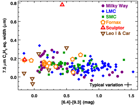
Figure 11.— The equivalent width of the absorption band from C₂H₂ at 7.5 $\mu$m as a function of the [6.4]$-$[9.3] color. The data point in the top center is MAG 29 in Sculptor. This spectrum has a 7.5 $\mu$m band more than twice as deep as any other measured. The general trend of stronger absorption bands with decreasing metallicity is most apparent for 0.5 $<$ [6.4]$-$[9.3] $<$ 1.0.

Table 11 presents the equivalent widths of the acetylene (C₂H₂) bands centered at 7.5 $\mu$m and 13.7 $\mu$m. As with Table 10, we do not quote the central wavelength if the S/N ratio of the equivalent width is less than 2.5. In addition, we omit it if the uncertainty in the wavelength exceeds 0.2 $\mu$m at 7.5 $\mu$m or 0.10 $\mu$m at 13.7 $\mu$m. In the cases with no central wavelength in Table 11, the equivalent width of the feature plus the uncertainty could be considered as an upper limit.

The 7.5 $\mu$m band arises from the P and R branches of the $\nu_{4}^{1}+\nu_{5}^{1}$ transitions and often presents a double-troughed structure with a central peak at 7.5 $\mu$m. The sharp absorption feature at 13.7 $\mu$m arises from the Q branch of the $\nu_{5}$ transition, primarily the fundamental mode, but with some contribution from higher overtones. The P and R branches extend this feature to cover the $\sim$13–15 $\mu$m range, but our lack of LL coverage prevents us from measuring the full band. Table 11 presents the equivalent width of just the Q branch at 13.7 $\mu$m. Matsuura et al. (2006) found that HCN, which often produces bands in the immediate vicinity of the C₂H₂ bands in Galactic carbon stars, was absent in the spectra of carbon stars in the LMC. This conclusion also applies to carbon stars in the SMC (Sloan et al., 2006). No evidence of HCN appears in the Local Group spectra presented here, but we note that limited S/N ratios and wavelength coverage at 14 $\mu$m prevent us from drawing any firm conclusions.

The wavelengths in Table 9 were used for all features except one, the 7.5 $\mu$m band in MAG 29. That band is so strong that the continuum wavelengths fall in the wings of the absorption, forcing us to shift them to 6.14–6.44 $\mu$m on the blue side and 9.12–9.52 $\mu$m to the red. It is also possible that the extension of the absorption to longer wavelengths is due to another molecule, but that molecule would probably be another hydrocarbon and thus trace the same molecular hydrocarbon mix as the acetylene feature.

We have detected a 7.5 $\mu$m band in most of our spectra. The exceptions include all three carbon stars in Carina as well as For DK 52. All of the spectra with detections show a clear minimum in the wavelength range covered by the band, although the noise can be considerable in some cases, due most likely to mismatches in the individual nod spectra and non-gaussian contributions which become a problem at these low flux levels.

The narrow 13.7 $\mu$m band is more difficult to detect. In addition to the lower signals at these wavelengths, only two of the spectra have LL data, leaving only three data points in SL for fitting the red continuum for the rest of the spectra, since we do not use SL past 14.17 $\mu$m. Nonetheless, we still detect a 13.7 $\mu$m band in seven of the 19 spectra, an impressive result given the sub-mJy strengths of most of the spectra at 14 $\mu$m.

All of our sources in Sculptor, Fornax, and Carina have been confirmed as carbon stars in the literature. Held et al. (2010) describe two of the three targets in Leo I, MFT C and A, as probable carbon stars. MFT C shows a convincingly strong 7.5 $\mu$m absorption band, and the 11.2 $\mu$m emission feature, while noisy, shows a shape consistent with SiC, allowing us to confirm its carbon-rich nature. MFT A also has a strong 7.5 $\mu$m band, although it is noisy. Given the lack of any obvious features at 11.3 and 13.7 $\mu$m, this object remains an unconfirmed carbon star. The chemistry of MFT E is less clear in the literature. The IRS spectrum shows what is best described as a weak, but noisy, 7.5 $\mu$m acetylene band and an emission feature at 11.3 $\mu$m consistent with SiC, which leads us to treat it as a probable, but unconfirmed carbon star.

We will focus on the 7.5 $\mu$m absorption band from C₂H₂ due to its better S/N ratio. Figure 11 plots its equivalent width vs. [6.4]$-$[9.3] color, allowing us to compare the molecular band strength at similar overall dust contents. The differences between the samples are most apparent in the color range 0.5–1.0, with a clear trend in increasing band strength from the Galaxy to the LMC to the SMC. Again, the three equivalent widths from Fornax are generally consistent with the Magellanic sample. Two of the three are among the strongest bands in this color range.

The data from the other dwarf galaxies are outside this color range, but a couple of comments are in order. First, MAG 29 in Scl has an equivalent width more than twice as strong as anything else in the sample. Menzies et al. (2011) noted that the IRS spectrum was obtained at maximum luminosity, which might account for the strong acetylene absorption. Even if this band varied by a factor of two over a pulsation cycle, it would still be stronger when at its minimum than in any other spectrum considered here. Second, two of the three stars in Leo I are among the strongest absorbers at 7.5 $\mu$m. The strong acetylene absorption in MAG 29 and in Leo I is consistent with the metal-poor nature of Sculptor and Leo I.

5.5. Metallicity diagnostics

Table 12Mean SiC and acetylene strengths

Galaxy	Number	$<$SiC/cont.$>$	$<$$7.5~{}{\rm\mu m}\$EW$>$
Milky Way	8	0.29 $\pm$ 0.07	0.06 $\pm$ 0.04
LMC	23	0.11 $\pm$ 0.07	0.08 $\pm$ 0.05
SMC	12	0.08 $\pm$ 0.06	0.12 $\pm$ 0.05
For dSph	3	0.12 $\pm$ 0.06	0.16 $\pm$ 0.10

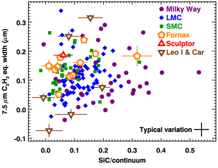
Figure 12.— The equivalent width of the acetylene band at 7.5 $\mu$m plotted as a function of the SiC/continuum emission ratio. MAG 29 is missing from this plot because it is so far above the rest of the data, with EW = 0.78 $\mu$m and SiC/cont. = 0.03. Lagadec et al. (2008) proposed this comparison as a metallicity diagnostic (their Fig. 11).

Table 12 summarizes the mean and standard deviation of the strength of the SiC emission (normalized to the continuum) and the equivalent width of the 7.5 $\mu$m acetylene absorption band. Both of these quantities vary with [6.4]$-$[9.3] color, and the various samples considered are incomplete at some colors. Consequently, we limit the comparison to the range 0.5 $<$ [6.4]$-$[9.3] $\leq$ 0.8. From the Milky Way to the LMC to the SMC, the trend of decreasing SiC strength and increasing C₂H₂ strength is clear. It is possible that the overlapping spreads in the data arise from a range of metallicities within the three galaxies. As described above (§ 2.2 and 4.2), we suspect that the metallicity of Fornax is closer to Magellanic than to the other dwarf spheroidal galaxies considered here. We have only three spectra in this color range, and they give ambiguous results. The SiC feature suggests a similarity to the LMC, but the spread in acetylene strengths limits our conclusions.

Lagadec et al. (2008) proposed plotting the two quantities in Table 12 against each other to diagnose metallicity. Figure 12 follows that lead. While the sample from each galaxy shows considerable scatter, the gradient is unmistakable, with the Galaxy dominating in the lower right, the LMC in the middle, and the SMC in the upper left. The Fornax spectra are distributed much like the SMC spectra. As explained above, the one discrepant point in Fornax is For DI 2, which might have PAHs, not SiC, in its spectrum. Overall, Figure 12 reinforces our suspicions about Fornax and suggests that it and the SMC have similar metallicity distributions.

The Sculptor data keep to the metal-poor side of the diagram, with MAG 29 literally off the charts (not plotted, with SiC/cont. = 0.03 and EW = 0.78 $\mu$m). This behavior is fully consistent with the narrow and metal-poor MDF for Sculptor. The three Carina spectra are clustered in the lower left, where metallicity is indeterminant. The Leo I data are more of a puzzle. Two of the three spectra are in the upper left, where we would expect them from the metallicity of their host galaxy, but Leo I MFT E lands squarely among the metal-rich spectra. This might indeed indicate a higher initial metallicity, but it may also suggest that a bit of caution is warranted with these data. One alternative explanation is that this spectrum is affected by strong C₃ absorption at 10 $\mu$m, which would push our continuum fit downward and enhance the apparent strength of the SiC emission.

6. Discussion

6.1. Carbon dust content and metallicity 

The most surprising result of this study is that the carbon stars in Sculptor and Leo I seem to have less dust around them than their counterparts in more metal-rich galaxies. Previous studies of carbon stars in the Galaxy, the LMC, and the SMC showed that the amount of circumstellar dust, as measured by the [6.4]$-$[9.3] color, followed the same relationship with pulsation period of the star, despite their differences in metallicity. The six carbon stars in Fornax with known pulsation periods also follow this relation. As explained in § 4.2, we believe that these stars have metallicities similar to those in the LMC and SMC. The two carbon stars in Sculptor, for which we estimate [Fe/H]$\sim$$-$1.0, and the three carbon stars in Leo I, with [Fe/H]$\sim$$-$1.35, are shifted downward on average about 0.19 magnitudes in Figure 8. This difference corresponds to a factor of two in dust production ($\dot{D}$, Equation 1).

The scatter in Figure 8 is considerable. The standard deviation about the fitted line corresponds to a range in $\dot{D}$ of a factor of 2.2 (up or down). The cause of this wide envelope around the general proportionality of dust content to pulsation period is an open question. A more careful look at the Magellanic data rules out luminosity (Sloan et al., in preparation). Metallicity also does not work, even though we expect a fairly broad range of metallicities within each of the Milky Way, LMC, and SMC. If metallicity were responsible, it would lead to a measurable shift in the mean dust content between each galaxy, which we do not see.

The data leave us to conclude that for [Fe/H] $\gtrsim$ $-$0.7, the amount of carbon-rich circumstellar dust shows no relation to the metallicity. The remainder of the discussion focuses on the implications. As stated in § 5.2 above, the carbon dust content is measured by the [6.4]$-$[9.3] color, with no assumptions about outflow velocity or gas-to-dust ratio.

6.2. C/O ratio and metallicity 

For a carbon star, the dust content depends primarily on the abundance of C, which it produces via the 3-$\alpha$ sequence and dredges to its surface. The free carbon available for dust production depends on what remains after CO consumes the available oxygen, so that

$$\frac{C_{\rm free}}{O}=\frac{C}{O}-1.$$ (3)

In this equation and the ones that follow, “C” and “O” are the fractional abundances of carbon and oxygen, by number. Not all of the free carbon will form dust; some of it appears in our spectra as acetylene, and other carbon-bearing molecules are possible. Because our carbon stars are embedded in dust and their distances make them faint, they are difficult targets for the high-resolution optical spectroscopy usually used to determine C/O ratios. While waiting for that problem to be solved, we can still estimate what C/O ratios we should expect. We can write

$$\frac{C}{O}=\frac{C_{i}+\delta C}{O}=\left(\frac{C}{O}\right)_{i}+\left(\frac{\delta C}{O_{i}}\right),$$ (4)

where $C_{i}$ is the initial carbon abundance, $\delta C$ is the change in abundance due to dredge-up, and we have assumed that the oxygen abundance does not change from its initial level.

Observations of the C/O ratio in dwarf galaxies reveal a decrease in C/O with decreasing metallicity (Garnett et al., 1995; Kobulnicky & Skillman, 1998, where O/H serves as a proxy for metallicity). This is the initial C/O ratio prior to any dredge-up on the AGB. Data from stellar spectroscopy in the Galaxy compiled by Chiappini et al. (1999, 2003) show no significant trend in [C_i/Fe] with [Fe/H]. The scatter is substantial, $\sim$0.2 dex, and the point is not without controversy, but we will assume no systematic relation between [C_i/Fe] and [Fe/H]. Similar spectroscopy by Mélendez & Burbuy (2002, and references therein) shows that a steadily increasing [O/Fe] ratio in more metal-poor samples is the culprit behind the changing (C/O)_i ratio. We estimate that in the range $-$1.5 $\lesssim$ [Fe/H] $\leq$ 0.0, [O/Fe] increases 0.25 dex for every decrease of 1 dex in [Fe/H]. The scatter about this trend is $\sim$0.1 dex on average. Applying this trend to the above equation gives:

$$\frac{C}{O}=\left(\frac{C}{O}\right)_{\odot}\left(10^{0.25\,{\rm[Fe/H]}}+\delta C\,10^{-0.75\,{\rm[Fe/H]}}\right).$$ (5)

The first term in the right-most parentheses is just the initial C/O ratio, which decreases by a factor of 1.78 for every dex in [Fe/H].

Let us assume that the amount of dredged up carbon ($\delta C$) does not vary significantly with metallicity. The arguments which follow will pursue the consequences and show that in fact this assumption is probably invalid.

For the sake of argument, we will also assume that a typical C/O ratio for a carbon star at solar metallicity is $\sim$1.1 (following Lagadec & Zijlstra, 2008, but see also Ohnaka et al. 2000). At solar metallicity, the initial C/O ratio of a star would be 0.54 (Asplund et al., 2005). To raise the C/O ratio to 1.1, $\delta C$ would have to be 0.56 O_⊙. Keeping this quantity fixed with metallicity leads to a C/O ratio at analogous stages of AGB evolution of 1.4 at [Fe/H] = $-$0.3 (i.e. in the LMC), 2.2 at [Fe/H] = $-$0.7 (SMC), and 3.5 at [Fe/H] = $-$1.0 (Sculptor).

Dividing Equation (2) by (C/O)_⊙ leads to a relation for the free carbon as a fraction of the total initial carbon at solar metallicity:

$$\frac{C_{\rm free}}{C_{\odot}}=\left(\frac{C}{O}-1\right)1.85\times 10^{0.75\,{\rm[Fe/H]}}.$$ (6)

For a star of solar metallicity, $C_{\rm free}$ = 0.19 $C_{\odot}$ (in this particular case, $C_{\odot}$ is the amount of carbon the star formed with). The corresponding values for the LMC, SMC, and Sculptor are 0.44, 0.68, and 0.81. It is instructive to consider the example of the SMC. Despite the fact that stars in the SMC form with only 20% of the carbon in their Galactic counterparts, if they dredge up the same amount of carbon, they will have 3.6 times more carbon free to form dust. This is a direct result of the reduced oxygen abundance, which limits how much carbon is sequestered as CO. All things being equal, we would expect to see more carbon-rich dust at lower metallicities, and yet, our measurements of the carbon dust content remain relatively constant with metallicity. We even see a possible dip at the metal-poor end of our sample.

6.3. Acetylene, the carbon budget, and mass-loss triggers

Before giving up on our assumption that $\delta C$ does not depend on metallicity, we should consider what might happen to this excess of free carbon at low metallicity. If the dust content stays flat or even falls, some other reservoir must be absorbing the carbon. SiC represents only trace amounts, but the strengthening acetylene bands at lower metallicity could be a solution.

Table 12 shows that the mean strength of the 7.5 $\mu$m acetylene band is twice as strong in the SMC than in the Milky Way, although the spread of the data about these means is considerable. If the 7.5 $\mu$m acetylene band accurately traces the total carbon mass in gaseous hydrocarbon molecules, then it follows from Table 12 that hydrocarbon gases sequester two times more carbon in the typical carbon star in the SMC compared to the Milky Way.

While this is a significant amount of carbon in gaseous form, it is not enough to account for the factor of 3.6 more free carbon expected in the SMC. We know of no other likely reservoir for the carbon, leading us to conclude that the amount of dredged up carbon ($\delta C$) must in fact decrease at lower metallicity. Neither the rate at which the triple-$\alpha$ sequence produces carbon nor the dredge-up efficiency should decrease at lower metallicity. To reduce $\delta C$, it is necessary to terminate the dredge-up process progressively earlier on the AGB in more metal-poor stars.

Models by Woitke (2006) show that the opacity of carbon-rich dust is sufficient to drive the mass-loss process. If a dredge-up event during a thermal pulse drives the C/O ratio high enough, then the jump in free carbon will lead to a pulse of dust formation which could quickly strip the envelope and bring the AGB evolution to a rapid end. Lagadec & Zijlstra (2008) proposed just such a scenario, although their definition of the free carbon differs from ours. The key point is that the trigger is not the C/O ratio, but the quantity of free carbon, modified, if seeds are important to the condensation process, by the abundances of elements such as Ti and perhaps Si. A spectroscopic census of the Sgr dSph galaxy (McDonald et al., in preparation) finds that the typical lifetime of a star as a carbon star may be similar to the time between thermal pulses. Once a star develops a carbon-rich envelope, the formation of dust and the loss of mass accelerates quickly.

6.4. Si, seeding, and abundance

Van Loon et al. (2008) explained the increasing acetylene band strengths in more metal-poor stars as a consequence of the lower abundances of elements like Ti. The lower abundances would result in fewer available seeds like TiC for the condensation of amorphous carbon dust, making the process less efficient.

SiC could play a similar role as a condensation seed. Sloan et al. (2006) suggested that the decreasing SiC emission at lower metallicity would arise naturally from decreasing Si abundances. Lagadec et al. (2007) and Leisenring et al. (2008) developed this idea, explaining the different tracks of SiC emission strength with [6.4]$-$[9.3] color in Figure 10 in the different samples as an increasingly delayed condensation of SiC with decreasing metallicity. Other seeds requiring heavy elements should behave similarly with decreasing metallicity. Without these seeds at lower metallicities, the less efficient formation of amorphous carbon is likely to result in a greater fraction of the free carbon tied up in simpler molecules like acetylene.

Observations of Magellanic planetary nebulae (PNe) by Bernard-Salas et al. (2009) create one difficulty for the idea that the reduced SiC strength in metal-poor carbon stars arises from reduced Si abundances. They found that strong emission features centered at $\sim$11 $\mu$m in several spectra, and they attributed these features to SiC. We suspect that the 11 $\mu$m feature in their PN spectra does not arise from SiC, but instead from a different carrier. The PN features are triangular in shape and peak at $\sim$11.1 $\mu$m, compared to the more rounded SiC features which peak at $\sim$11.3 $\mu$m. Additionally, the PN features are usually associated with features at $\sim$16 $\mu$m. Both the 11 and 16 $\mu$m features are often seen in spectra showing the still unidentified 21 $\mu$m feature (Kraemer et al., 2002, Sloan et al. in preparation).

6.5. Gas-to-dust ratio and outflow velocity

For evolved oxygen-rich stars, the gas-to-dust ratio should depend strongly on metallicity, because the abundances of the elements which form oxygen-rich dust scale with metallicity (e.g., van Loon, 2000). The outflow velocity depends on the radiation pressure on the dust and its coupling to the gas due to collisions, and it should also vary with metallicity.

The situation for carbon stars is different, because they produce the carbon which drives the mass-loss themselves. The spectra in this paper show that if the dust content decreases with lower metallicity, the dependence is weak and noticeable only for the most metal-poor stars observed. Following the carbon budget leads us to the same conclusion as Lagadec & Zijlstra (2008), that the free carbon serves as a trigger for the superwind phase.

The lack of a strong dependence of carbon-rich dust content with metallicity makes it difficult to see how the gas-to-dust ratio or the outflow velocity should depend on metallicity. If radiation pressure accelerates the dust, and collisions between dust grains and gas molecules accelerate the gas, then the amount of dust would determine both outflow velocity and total mass-loss rate, and as we have shown, the amount of dust does not vary strongly with metallicity. If pulsations drive the mass-loss process, then the mass-loss rate will depend primarily on the pulsation period and amplitude, which are relatively insensitive to metallicity. Again, neither the outflow velocity nor the gas-to-dust ratio should depend strongly on metallicity.

A rigorous test of these predictions awaits observations from the Atacama Large Millimeter Array (ALMA). Less sensitive telescopes can be used to study carbon stars in the Galactic Halo. Lagadec et al. (2010) observed a sample of six carbon stars in the Halo and found that they have smaller outflow velocities than carbon stars in the Galactic disk. Lagadec et al. (2012) obtained infrared spectra of four of these carbon stars with the IRS, and they found evidence suggesting that halo Carbon stars also have high gas-to-dust ratios. Thus, both outflow velocity and gas-to-dust ratio may depend on metallicity for carbon stars, after all, but some caution is in order. First, the metallicity of the observed carbon stars is uncertain; they may be ejected from the Galactic disk. Second, if the outflow velocity of the dust is higher than the gas, then the inferred gas-to-dust ratios may not differ from the disk sample as much. The Halo carbon stars raise some interesting possibilities, but these initial results require follow-up.

The review of CO line observations in Galactic carbon stars by Schöier (2007) shows a range of possible outflow velocities, from a few km/s to over 20 km/s, with higher outflow velocities generally associated with higher total mass-loss rates. The relation between outflow velocity and total mass-loss rate is consistent with increasing amounts of circumstellar dust, which leads to more efficient acceleration of the circumstellar envelope. Metallicity is not needed to explain the effect, even if the range of possible outflow velocities does inject a degree of caution when using Equation (1) or interpreting the mass-loss rates presented in Table 10.

7. Summary

The sample of carbon stars beyond the Magellanic Clouds observed by the IRS on Spitzer consists of 19 stars in the Sculptor, Carina, Fornax, and Leo I dwarf spheroidal galaxies. The invidual targets were chosen based on their red NIR colors or their pulsation properties. The bolometric magnitudes of the two targets in Sculptor, their pulsation periods, and reference to recent modelling work lead us to revise their estimated metallicity ([Fe/H]) up to $\sim$$-$1.0. Similarly, we suggest that the carbon stars in Fornax have metallicities more similar to the LMC and SMC than to the other dwarfs studied. The mean metallicity in Leo I and Carina are $\sim$ $-$1.4 and $-$1.7, respectively.

All carbon stars follow a general relation of increasing dust content as the pulsation period increases. Metallicity does not show any influence down to [Fe/H]$\sim$$-$0.7, so that despite their differences in initial metallicity, carbon stars in the Galaxy, LMC, SMC, and Fornax with similar pulsation periods produce similar quantities of dust. The five stars observed in Sculptor and Leo I produce less dust, at a significance level of 3.6 $\sigma$. The carbon stars in Carina show no dust, but lack of pulsation periods prevent us from comparing them to the stars in the other galaxies.

The new carbon stars extend the previously detected trends of decreasing emission from SiC dust and increasing absorption from acetylene gas as the metallicity falls to even lower metallicities. The carbon stars in Fornax show SiC features and acetylene bands consistent with our revised metallicity.

If the quantity of freshly produced carbon from the stellar interior to the photosphere does not depend on metallicity, the lower initial abundances of oxygen in more metal-poor stars would lead to substantially greater quantities of free carbon. Yet, as our observations have shown, they do not produce substantially larger amounts of amorphous carbon dust. While more metal-poor stars do produce more acetylene gas, it is not enough to account for the expected increases of free carbon. We conclude that some process must truncate the dredge-up earlier in more metal-poor samples, quite likely a superwind triggered by a free-carbon threshold which strips the star of its envelope and ends its evolution on the AGB.

Because the amount of circumstellar carbon-rich dust observed does not depend strongly on the metallicity, we should not expect any strong dependencies of outflow velocity or gas-to-dust ratio on metallicity as well.

References

- Aaronson & Mould (1980) Aaronson, M., & Mould, J. 1980, ApJ, 240, 804
- Aaronson & Mould (1985) Aaronson, M., & Mould, J. 1985, ApJ, 290, 191
- Abia et al. (2008) Abia, C., de Laverny, P., & Wahlin, R. 2008, A&A, 481, 161
- Asplund et al. (2005) Asplund, M., Grevesse, N., & Sauval, A. J. 2005, in Cosmic Abundances as Records of Stellar Evolution and Nucleosynthesis, ed., F. N. Bash, & T. G. Barnes, ASP Conf. Series, 336, 25 (San Francisco: ASP)
- Azzopardi et al. (1985) Azzopardi, M., Lequex, J., & Westerlund, B. E. 1985, A&A, 144, 388
- Azzopardi et al. (1986) Azzopardi, M., Lequex, J., & Westerlund, B. E. 1986, A&A, 161, 232
- Azzopardi et al. (1999) Azzopardi, M., Muratorio, G., Breysacher, J., & Westerlund, B. E. 1999, in The Stellar Content of Local Group Galaxies, Proc. IAU Symp. 192, ed. P. Whitelock, & Cannon, R., 144 (San Francisco: PASP)
- Battaglia et al. (2006) Battaglia, G., et al. 2006, A&A, 459, 423
- Beichman et al. (1988) Beichman, C. A., Neugebauer, G., Habing, H. J., Clegg, P. E., & Chester, T. J. 1988, Infrared astronomical satellite (IRAS) catalogs and atlases. Volume 1: Explanatory supplement
- Bellazzini et al. (2004) Bellazzini, M., Gennari, N., Ferraro, F. R., & Sollima, A. 2004, MNRAS, 354, 708
- Bernard-Salas et al. (2009) Bernard-Salas, J., Peeters, E., Sloan, G. C., Gutenkunst, S., Zijlstra, A. A., Matsuura, M., Tielens, A. G. G. M., & Houck, J. R. 2009, ApJ, 699, 1541.
- Bersier (2000) Bersier, D. 2000, ApJ, 543, L23
- Bersier & Wood (2002) Bersier, D., & Wood, P. R. 2002, AJ, 123, 840
- Bessell & Wood (1984) Bessell, M. S., & Wood, P. R. 1984, PASP, 96, 247
- Blanco et al. (1978) Blanco, B. M., Blanco, V. M., & McCarthy, M. F. 1978, Nature, 271, 638
- Blanco et al. (1980) Blanco, V. M., Blanco, B. M., & McCarthy, M. F. 1980, ApJ, 242, 938
- Bono et al. (2010) Bono, G., et al. 2010, PASP, 122, 651
- Bosler et al. (2007) Bosler, T. L., Smecker-Hane, T. A., & Stetson, P. B. 2007, MNRAS, 378, 318
- Boyer et al. (2012) Boyer, M. L., Srinivasan, S., Riebel, D., McDonald, I., van Loon, J. Th., Clayton, G. C., Gordon, K. D., Meixner, M., Sargent, B. A., & Sloan, G. C. 2012, ApJ, 748, 40
- Buchanan et al. (2006) Buchanan, C. L., Kastner, J. H., Forrest, W. J., Hrivnak, B. J., Sahai, R., Egan, M., Frank, A., & Barnbaum, C. 2006, AJ, 132, 1890
- Buonanno et al. (1985) Buonanno, R., Corsi, C. E., Fusi Pecci, F., Hardy, E., & Zinn, R. 1985, A&A, 152, 65
- Buonanno et al. (1999) Buonanno, R., Corsi, C. E., Castellani, M., Marcano, G., Fusi Pecci, F., & Zinn, R. 1999, AJ, 118, 1671
- Cannon et al. (1977) Cannon, R. D, Hawarden, T. G., & Tritton, S. B. 1977, MNRAS, 180, 81P
- Caputo et al. (1999) Caputo, F., Cassisi, S., Castellani, M., Marconi, G., & Santolamazza, P. 1999, AJ, 117, 2199
- Carretta & Gratton (1997) Carretta, E., & Gratton, R. G. 1997, A&AS, 121, 95
- Chiappini et al. (1999) Chiappini, C., Matteucii, F., Beers, T. C., & Nomoto, K. 1999, ApJ, 515, 226
- Chiappini et al. (2003) Chiappini, C., Romano, D., Matteucci, F. 2003, MNRAS, 339, 63
- Cioni & Habing (2003) Cioni, M.-R. L. & Habing, H. J. 2003, A&A, 402, 133
- Cohen, et al. (2003) Cohen, M., Wheaton, W. A., & Megeath, S. T. 2003, AJ, 126, 1090
- Coleman & de Jong (2008) Coleman, M. G., & de Jong, J. T. A. 2008, ApJ, 685, 933
- Dall’Ora et al. (2003) Dall’Ora, M., Ripepi, V., Caputo, F., Castellani, V., Bono, G., Smith, H. A.; Brocato, E., Buonanno, R., Castellani, M., Corsi, C. E., Marconi, M., Monelli, M., Nonino, M., Pulone, L., & Walker, A. R. 2003, AJ, 126, 197
- Demers & Irwin (1987) Demers, S., & Irwin, M. J. 1987, MNRAS, 226, 943
- Demers & Kunkel (1979) Demers, S., & Kunkel, W. E. 1979, PASP, 91, 761
- Demers et al. (1979) Demers, S., Kunkel, W. E., & Hardy, E. 1979, ApJ, 232, 84
- Demers et al. (1994) Demers, S., Irwin, M. J., & Gambu, I. 1994, MNRAS, 266, 7
- Demers et al. (2002) Demers, S., Dallaire, M., & Battinelli, P. 2002, AJ, 123, 3428
- Draine & Lee (1984) Draine, B. T., & Lee, H. M. 1984, ApJ, 285, 89
- Egan & Sloan (2001) Egan, M. P., & Sloan, G. C. 2001, ApJ, 558, 165
- Egan et al. (2003) Egan, M. P., et al. 2003, Air Force Research Laboratory Technical Report AFRL-VS-TR-2003-1589 (Hanscom AFB: USAF)
- Frogel et al. (1982) Frogel, J. A., Blanco, V. M., McCarthy, M. F., & Cohen J. G. 1982, ApJ, 252, 133
- Gallart et al. (1999) Gallart, C., Freedman, W. L., Aparicio, A. Bertelli, G., & Chiosi, C. 1999, AJ, 118, 2245
- Garnett et al. (1995) Garnett, D. R., Skillman, E. D., Dufour, R. J., Peimbert, M., Torres-Peimbert, S., Terlevich, R., Terlevich, E., & Shields, G. A. 1995, ApJ, 443, 64
- Gehrz (1989) Gehrz, R. 1989, in Interstellar Dust, Proc. IAU Symp. 135, ed. L. J. Allamandola, & A. G. G. M. Tielens (Dordrecht: Kluwer Academic Publishers), 445
- Greco et al. (2007) Greco, C., Clementini, G., Catelan, M., Held, E. V., Poretti, E., Gullieuszik, M., Maio, M., Rest, A., De Lee, N., Smith, H. A., & Pritzl, B. J. 2007, ApJ, 670, 332
- Groenewegen et al. (2007) Groenewegen, M. A. T., et al. 2007, MNRAS, 376, 313
- Groenewegen et al. (2009a) Groenewegen, M. A. T., Lançon, A., & Marescaux, M. 2009, A&A, 504, 1031
- Groenewegen et al. (2009b) Groenewegen, M. A. T., Sloan, G. C., Soszyński, I., & Petersen, E. 2009b, A&A, 506, 1277
- Gullieuszik et al. (2007) Gullieuszik, M., Held, E. V., Rizzi, L., Saviane, I., Momany, Y., & Ortolani, S. 2007, A&A, 467, 1025
- Gullieuszik et al. (2009) Gullieuszik, M., Held, E. V., Saviane, I., & Rizzi, L. 2009, A&A, 500, 735
- Habing (1996) Habing, H. J. 1996, Astron. & Astrophys. Rev., 7, 97
- Harrington & Wilson (1950) Harrington, R. G., & Wilson A. G. 1950, PASP, 62, 118
- Held et al. (2001) Held, E. V., Clementini, G., Rizzi, L., Momany, Y., Saviane, I., & Di Fabrizio, L., 2001, ApJ, 562, L39
- Held et al. (2010) Held, E. V., Gullieuszik, M., Rizzi, L., Girardi, L., Marigo, P., & Saviane, I. 2010, MNRAS, 1475
- Helmi et al. (2006) Helmi, A., et al. 2006, ApJ, 651, L121
- Houck et al. (2004) Houck, J. R., et al. 2004, ApJS, 154, 18
- Hurley-Keller et al. (1998) Hurley-Keller, D., Mateo, M., & Nemec, J. 1998, AJ, 115, 1840
- Hurley-Keller et al. (1999) Hurley-Keller, D., Mateo, M., & Grebel, E. K. 1999, ApJ, 523, L25
- Iben & Renzini (1983) Iben, I., Jr., & Renzini, A. 1983, ARA&A, 21, 272
- Irwin & Hatzidimitriou (1995) Irwin, M., & Hatzidimitriou, D. 1995, MNRAS, 277, 1354
- Kaluzny et al. (1995) Kaluzny, J., Krzemiński, W., & Mazur, B. 1995, AJ, 110, 2206
- Kamath et al. (2011) Kamath, D., Karakas, A. I., & Wood, P. R. 2011, ApJ, in press
- Karakas & Lattanzio (2007) Karakas, A., & Lattanzio, J. C., Publ. of the Astron. Soc. of Australia, 24, 103
- Kirby et al. (2009) Kirby, E. N., Guhathakurta, P., Bolte, M., Sneden, C., & Geha, M. C. 2009, ApJ, 705, 328
- Kobulnicky & Skillman (1998) Kobulnicky, H. A., & Skillman, E. D. 1998, ApJ, 497, 601
- Koch et al. (2006) Koch, A., Grebel, E. K., Wyse, R. F. G., Kleyna, J. T., Wilkinson, M. I., Harbeck, D. R., Gilmore, G. F., & Evans, N. W. 2006, AJ, 131, 895
- Koch et al. (2007) Koch, A., Wilkinson, M. I., Kleyna, J. T., Gilmore, G. F., Grebel, E. K., Mackey, A. D., Evans, N. W., & Wyse, R. F. G. 2007, ApJ, 657, 241
- Koch et al. (2008) Koch, A., Grebel, E. K., Gilmore, G. F., Wyse, R. F. G., Kleyna, J. T., Harbeck, D. R., Wilkinson, M. I., & Evans, N. W. 2008, AJ, 135, 1580
- Kraemer et al. (2002) Kraemer, K. E., Sloan, G. C., Price, S. D., & Walker, H. J. 2002, ApJS, 140, 389
- Lagadec et al. (2007) Lagadec, E., Zijlstra, A. A., Sloan, G. C., Matsuura, M., Wood, P. R., van Loon, J. Th., Harris, G. J., Blommaert, J. A. D. L., Hony, S., Groenewegen, M. A. T., Feast, M. S., Whitelock, P. A., Menzies, J. W., & Cioni, M.-R. 2007, MNRAS, 376, 1270
- Lagadec et al. (2008) Lagadec, E., Zijlstra, A. A., Matsuura, M., Menzies, J. W., van Loon, J. Th., & Whitelock, P. A. 2008, MNRAS, 383, 399
- Lagadec & Zijlstra (2008) Lagadec, E., & Zijlstra, A. A. 2008, MNRAS, 390, L59
- Lagadec et al. (2009) Lagadec, E., Zijlstra, A. A., Sloan, G. C., Wood, P. R., Matsuura, M., Bernard-Salas, J, Blommaert, J. A. D. L., Cioni, M.-R. L., Feast, M. W., Groenewegen, M. A. T., Hony, S., Menzies, J. W., van Loon, J. Th., & Whitelock, P. A. 2009, MNRAS, 396, 598
- Lagadec et al. (2010) Lagadec, E., Zijlstra, A. A., Mauron, N., Fuller, G., Josselin, E., Sloan, G. C., & Riggs, A. J. E. 2010, MNRAS, 403, 1331
- Lagadec et al. (2012) Lagadec, E., Sloan G. C., Zijlstra, A. A., Mauron, N., & Houck, J. R. 2012, MNRAS, submitted
- Laor & Draine (1993) Laor, A., & Draine, B. T. 1993, ApJ, 402, 441
- Lasker et al. (2008) Lasker, B. M., et al. 2008, AJ, 136, 735 (Guide Star Catalog 2.3.2)
- Lebouteiller et al. (2010) Lebouteiller, V., Bernard-Salas, J., Sloan, G. C., & Barry, D. J. 2010, PASP, 122, 231
- Lebouteiller et al. (2011) Lebouteiller, V., Barry, D. J., Spoon, H. W. W., Bernard-Salas, J., Sloan, G. C., Houck, J.R., & Weedman, D. 2011, ApJS, 196, 8
- Lebzelter et al. (2006) Lebzelter, Th., Posch, Th., Hinkle, K., Wood, P. R., & Bouwman, J. 2006, ApJ, 653, L145
- Lee et al. (1993) Lee, M. G., Freedman, W., Mateo, M., Thompson, I., Roth, M., & Ruiz, M.-T. 1993, AJ, 106, 1420
- Leisenring et al. (2008) Leisenring, J. M., Markwick-Kemper, F., & Sloan, G.C. 2008, ApJ, 681, 1577
- Lépine et al. (2011) Lépine, S., Koch, A., Rich, R. M., & Kuijken, K. 2011, ApJ, 741, 100
- Mackey & Gilmore (2003) Mackey, A. D., & Gilmore, G. F. 2003, MNRAS, 343, 747
- Majewski et al. (1999) Majewski, S. R., Siegel, M. H., Patterson, R. J., & Rood, R. T. 1999, ApJ, 520, L33
- Maraston (2005) Maraston, C. 2005, MNRAS, 362, 799
- Martin & Rogers (1987) Martin, P. G., & Rogers, C. 1987, ApJ, 322, 374
- Mateo et al. (1998) Mateo, M., Hurley-Keller, D., & Nemec, J. 1998, AJ, 115, 1856
- Mattsson et al. (2008) Mattsson, L., Wahlin, R., Höfner, S., & Eriksson, K. 2008, A&A, 484 L5
- Matsuura et al. (2006) Matsuura, M., et al. 2006, MNRAS, 371, 415
- Matsuura et al. (2007) Matsuura, M., Zijlstra, A. A., Bernard-Salas, J., Menzies, J. W., Sloan, G. C., Whitelock, P. A., Wood, P. R., Cioni, M.-R. L., Feast, M. W., Lagadec, E., van Loon, J. Th., Groenewegen, M. A. T., & Harris, G. J. 2007, MNRAS, 382, 1889
- Matsuura et al. (2011) Matsuura, M., et al. 2011, Science, 333, 1258
- Matsuura (2012) Matsuura, M. 2012, MNRAS, submitted
- Mauron et al. (2004) Mauron, N., Azzopardi, M., Gigoyan, K., & Kendall, T. R. 2004, A&A, 418, 77
- McDonald et al. (2011) McDonald, I., van Loon, J. Th., Sloan, G. C., Dupree, A. K., Zijlstra, A. A., Boyer, M. L., Gehrz, R. D., Evans, A., Woodward, C. E., & Johnson, C. I. 2011, MNRAS, 417, 20
- Mélendez & Burbuy (2002) Mélendez, J. & Burbuy, B. 2002, ApJ, 575, 474
- Méndez et al. (2002) Méndez, B., Davis, M., Moustakas, J., Newman, J., Madore, B. F., & Freedman, W. L. 2002, AJ, 124, 213
- Menzies et al. (2002) Menzies, J., Feast, M., Tanabé, T., Whitelock, P., & Nakada, Y. 2002, MNRAS, 335, 932
- Menzies et al. (2010) Menzies, J. W., Whitelock, P. A., Feast, M. W., & Matsunaga, N. 2010, MNRAS, 406, 86
- Menzies et al. (2011) Menzies, J. W., Feast, M. W., Whitelock, P. A., & Matsunaga, N. 2011, MNRAS, 414, 3492
- Mighell (1990) Mighell, K. J. 1990, A&AS, 82, 1
- Monelli et al. (2003) Monelli, M., et al. 2003, AJ, 126, 218
- Monet et al. (2003) Monet, D. G., et al. 2003, AJ, 125, 984 (USNO-B Catalog)
- Mould et al. (1982) Mould, J. R., Cannon, R. D., Aaronson, M., & Frogel, J. A. 1982, ApJ, 254, 500
- Nagayama et al. (2003) Nagayama, T., Nagashima, C., Nakajima, Y., Nagata, T., Sato, S., Nakaya, H., Yamamuro, T., Sugitani, K., & Tomura, M. 2003, Proc. SPIE, 4841, 459
- Ohnaka et al. (2000) Ohnaka, K., Tsuji, T., & Aoki, W. 2000, A&A, 353, 528
- Onaka et al. (1989) Onaka, T., de Jong, T., & Willems, F. J. 1989, A&A, 218, 169
- Pietryzyński et al. (2003) Pietrzyński, G., Gieren, W., & Udalski, A. 2003, AJ, 125, 2494
- Pietryzyński et al. (2008) Pietrzyński, G., Gieren, W., Szewczyk, O., Walker, A., Rizzi, L., Bresolin, F., Kudritzki, R.-P., Nalewajko, K., Storm, J., Dall’Ora, M., & Ivanov, V. 2008, AJ, 135, 1993
- Pietryzyński et al. (2009) Pietrzyński, G., Górski, M., Gieren, W., Ivanov, V. D., Bresolin, F., & Kudritzki, R. P. 2009, AJ, 138, 459
- Pont et al. (2004) Pont, F., Zinn, R., Gallart, C., Hardy, E., & Winnick, R. 2004, AJ, 127, 840
- Renzini & Voli (1981) Renzini, A. & Voli, M. 1981, A&A, 94, 175
- Revaz et al. (2009) Revaz, Y., Jablonka, P., Sawala, T., Hill, V., Letarte, B., Irwin, M., Battaglia, G., Helmi, A., Shetrone, M. D., Tolstoy, E., & Venn, K. A. 2009, A&A, 501, 189
- Rieke et al. (2008) Rieke, G. H., Blaylock, M., Decin, L., Engelbracht, C., Ogle, P., Avrett, E., Carpenter, J., Cutri, R. M., Armus, L., Gordon, K., Gray, R. O., Hinz, J., Su, K., Willmer, C. N. A. 2008, AJ, 135, 2245
- Rieke & Lebofsky (1985) Rieke, G. H., & Lebofsky, M. J. 1985, ApJ, 288, 618
- Rizzi et al. (2007a) Rizzi, L., Tully, B., Makarov, D., Makarova, L., Dolphin, A. E., Sakai, S., & Shaya, E. J. 2007a, ApJ, 661, 815
- Rizzi et al. (2007b) Rizzi, L., Held, E. V., Saviane, I., Tully, R. B., & Gullieuszik, M. 2007b, MNRAS, 380, 1255
- Salpeter (1952) Salpeter, E. E. 1952, ApJ, 115, 326
- Saviane et al. (2000) Saviane, I., Held, E. V., Bertelli, G. 2000, A&A, 355, 56
- Schlegel et al. (1998) Schlegel, D. J., Finkbeiner, D. P., & Davis, M. 1998, ApJ, 500, 525
- Schöier (2007) Schöier, F. L., 2007, in Why Galaxies Care About AGB Stars: Their Importance as Actors and Probes, ed., F. Kerschbaum, C. Charbonnel, & R. F. Wing, ASP Conf. Series, 378, 216 (San Francisco: ASP)
- Shapley (1938) Shapley, H. 1938, Nature, 142, 715
- Skrutskie et al. (2006) Skrutskie, M. F., et al. 2006, AJ, 131, 1163
- Sloan et al. (2003) Sloan, G. C., Kraemer, K. E., Price, S. D., & Shipman, R. F. 2003, ApJS, 147, 379
- Sloan et al. (2006) Sloan, G. C., Kraemer, K. E., Matsuura, M., Wood, P. R., Price, S. D., & Egan, M. P. 2006, ApJ, 645, 1118
- Sloan et al. (2008) Sloan, G. C., Kraemer, K. E., Wood, P. R., Zijlstra, A. A., Bernard-Salas, J., Devost, D., & Houck, J. R. 2008, ApJ, 686, 1056
- Sloan et al. (2009) Sloan, G. C., Matsuura, M., Zijlstra, A. A., Lagadec, E., Groenewegen, M. A. T., Wood, P. R., Szyszka, C., Bernard-Salas, J., & van Loon, J. Th. 2009, Science, 323, 353
- Sloan et al. (2010) Sloan, G. C., Matsunaga, N., Matsuura, M., Zijlstra, A. A., Kraemer, K. E., Wood, P. R., Nieusma, J., Bernard-Salas, J., Devost, D., & Houck, J. R. 2010, ApJ, 719, 1274
- Smecker-Hane et al. (1994) Smecker-Hane, T. A., Stetson, P. B., Hesser, J. E., & Lehnert, M. D. 1994, AJ, 108, 507
- Smecker-Hane et al. (1996) Smecker-Hane, T. A., Stetson, P. B., Hesser, J. E., & Vandenberg, D. A. 1996, in From Stars to Galaxies: The Impact of Stellar Physics on Galaxy Evolution, ed. C. Leitherer, U. Fritze-von-Alvensleben, & J. Huchra, ASP Conf. Series, 98, 328 (San Francisco: ASP)
- Stetson et al. (1998) Stetson, P. B., Hesser, J. E., & Smecker-Hane, T. A. 1998, PASP, 110, 533
- Tolstoy et al. (2001) Tolstoy, E., Irwin, M. J., Cole, A. A., Pasquini, L., Gilmozzi, R., & Gallagher, J. S. 2001, MNRAS, 327, 918
- Tolstoy et al. (2004) Tolstoy, E., et al. 2004, ApJ, 617, L119
- van Agt (1978) van Agt, S. L. Th. J. 1978, Publ. David Dunlap Obs., 3, 205
- van Loon (2000) van Loon, J. Th. 2000, A&A, 354, 125
- van Loon et al. (2008) van Loon, J. Th., Cohen, M., Oliveira, J. M., Matsuura, M., McDonald, I., Sloan, G. C., Wood, P. R., & Zijlstra, A. A. 2008, A&A, 487, 1055
- Vassiliadis & Wood (1993) Vassiliadis, E., & Wood, P. R. 1993, ApJ, 413, 641
- Walker et al. (2009) Walker, M. G., Mateo, M., & Olszewski, E. W. 2009, AJ, 137, 3100
- Werner et al. (2004) Werner, M. W., et al. 2004, ApJS, 154, 1
- Westerlund et al. (1987) Westerlund, B. E., Edwardsson, B., & Lundgren, K. 1987, A&A, 178, 41
- Whitelock et al. (2006) Whitelock, P. A., Feast, M. W., Marang, F., & Groenewegen, M. A. T. 2006, MNRAS, 369, 751
- Whitelock et al. (2009) Whitelock, P. A., Menzies, J. W., Feast, M. W., Matsunaga, N., Tanabé, T., & Ita, Y. 2009, MNRAS, 394, 795
- Woitke (2006) Woitke, P. 2006, A&A, 452, 537
- Wood & Sebo (1996) Wood, P. R., & Sebo, K. M. 1996, MNRAS, 282, 958
- Zacharias et al. (2004) Zacharias, N., Monet, D. G., Levine, S. E., Urban, S. E., Gaume, R., & Wycoff, G. L. 2004, BAAS, 36, 1418 (USNO NOMAD Catalog)
- Zijlstra et al. (2006) Zijlstra, A. A., et al. 2006, MNRAS, 370, 1961