Diagnostics of Baryonic Cooling in Lensing Galaxies

Abstract

Theoretical studies of structure formation find an inverse proportionality between the concentration of dark matter haloes and virial mass. This trend has been recently confirmed for $M_{\textrm{\tiny{vir}}}\gtrsim 6\times 10^{12}M_{\odot}$ by the observation of the X-ray emission from the hot halo gas. We present an alternative approach to this problem, exploring the concentration of dark matter haloes over galaxy scales on a sample of 18 early-type systems. Our $c-M_{\textrm{\tiny{vir}}}$ relation is consistent with the X-ray analysis, extending towards lower virial masses, covering the range from $~{}4\times 10^{11}M_{\odot}$ up to $5\times 10^{12}M_{\odot}$. A combination of the lensing analysis along with photometric data allows us to constrain the baryon fraction within a few effective radii, which is compared with prescriptions for adiabatic contraction (AC) of the dark matter haloes. We find that the standard methods for AC are strongly disfavored, requiring additional mechanisms – such as mass loss during the contraction process – to play a role during the phases following the collapse of the haloes.

1 Introduction

Dark matter haloes constitute the scaffolding on which the luminous component of cosmic structure can be detected in the form of galaxies. The connection between ordinary matter (i.e. “baryons”) and the dominant dark matter can only be found indirectly because of the elusive nature of the latter. Theoretical studies give useful insight under a number of assumptions about the properties of the dark matter component. N-body simulations predict a universal density profile (Navarro et al., 1996) driven by two parameters, the mass of the halo – usually defined out to a virial radius – and the concentration, given as the ratio between the scale length of the halo ($r_{\textrm{\tiny{S}}}$, where $\Delta\log\rho/\Delta\log r=-2$) and the virial radius. A number of N-body simulations (see e.g. Bullock et al., 2001; Neto et al., 2007; Macciò et al., 2007) display a significant trend between these two parameters, mainly driven by the hierarchical buildup of structure. Massive haloes assemble at later epochs – when the background density is lower because of the expansion of the Universe. Hence, we expect a trend whereby concentration decreases with increasing galaxy mass. An observational confirmation of this theoretical result by means of model-independent mass reconstruction gives insights in the interplay between luminous and dark matter.

Over cluster scales it is possible to explore the dark matter halo via its effect on the gravitational potential. The X-ray bremsstrahlung emission from the hot gas in the intracluster medium acts as a tracer of the potential. If assumptions are made about the dynamical state of the cluster, one can constrain the halo properties (see e.g. Sato et al., 2000). Buote et al. (2007) found a significant correlation between dark matter halo and mass, as expected from theoretical studies. Their sample covers a range from massive early-type galaxies up to galaxy clusters. In this paper, we extend the observational effort towards lower masses, constraining the haloes over galaxy scales by the use of strong gravitational lensing. By targeting a sample of strong lenses at moderate redshift (z$\sim$0.5) we probe the mass distribution out to a few ($\sim$4) effective radii. Other approaches to probe dark matter haloes over galaxy scales involve the use of dynamical tracers such as the bulk of the stellar populations (Gerhard et al., 2001). While Sauron data, as used in Cappellari et al. (2006) is restricted to 1–2 effective radii by the surface brightness detection limit of the observations and contains thus little information on the properties of the halos, studies based on more extended data are available (see e.g. Thomas et al., 2009). Additionally, planetary nebulæ in the outer regions of galaxies (Hui et al., 1995; Romanowsky et al., 2003; Deason et al., 2011) or globular clusters (Côté et al., 2001; Romanowsky et al., 2009; Schuberth et al., 2010) make it possible to probe the dark matter profile. Being evolved phases of the underlying stellar populations, planetary nebulæ can be considered unbiased tracers of the gravitational potential (see e.g. Coccato et al., 2009). Through their emission lines, it is possible to trace their kinematics out to large distances, reaching out to $\sim 5R_{\textrm{\tiny{e}}}$(Douglas et al., 2002). However, the interpretation of the results is difficult because of the uncertainties regarding the parameterisation of the halo mass, anisotropy, shape, or inclination (de Lorenzi et al., 2009). Gravitational lensing studies do not suffer from the inherent degeneracies of methods regarding the modelling of the dynamical tracers, although it is fair to say that lensing studies have other modelling degeneracies, as we discuss in the following Section. Ultimately, a comparison between all these methods is key to a robust assessment of the $c-M_{\textrm{\tiny{vir}}}$ relation.

Our recent study of stellar and total mass in lensing galaxies (Leier et al., 2011, hereafter LFSF) indicated an inverse trend of concentration with mass. Those results, however, applied to radii much smaller than the virial radius $r_{\textrm{\tiny{vir}}}$. In this work, we extend this analysis by extrapolating the inferred dark-matter profiles out to $r_{\textrm{\tiny{vir}}}$, to determine whether the concentration/mass trend persists to lower masses, i.e., galaxy haloes. We then try to reconstruct the possible concentrations of the dark-matter haloes before adiabatic contraction due to the baryons.

We consider a sample of 18 early-type lensing galaxies. In LFSF these galaxies (plus two disk galaxies and one ongoing major merger) were decomposed into stellar and dark-matter profiles. The stellar-mass or $M_{\textrm{\tiny{stel}}}$ profiles were obtained by fitting stellar population synthesis models to the star light. The lensing-mass or $M_{\textrm{\tiny{lens}}}$ profiles were obtained from lens models. The difference between these is assumed to be the dark-matter profile.

In Section 2 of the present paper we summarize the method of deriving the dark-matter profile as $M_{\textrm{\tiny{lens}}}-M_{\textrm{\tiny{stel}}}$. We also consider the technique of simply fitting a two-component lens model. The latter technique, in a test case (see Fig. 1) appears adequate for estimating $M_{\textrm{\tiny{lens}}}$ but significantly overestimates $M_{\textrm{\tiny{stel}}}$.

In Section 3 we fit well-known NFW and Hernquist profiles to the dark and stellar-mass profiles respectively. Figure 2 shows the NFW and Hernquist parameter estimates and uncertainties for two of the galaxies, while Figure 3 shows the dark-matter profiles for the same two galaxies. The NFW fits automatically provide a virial mass $M_{\textrm{\tiny{vir}}}$ and a concentration $c$, in effect extrapolating the dark-matter profile out to the virial radius $r_{\textrm{\tiny{vir}}}$. Figure 4 shows $M_{\textrm{\tiny{vir}}}$ and $c$ for all 18 galaxies. The trend shown in Buote et al. (2007) is seen to extend down to virial masses of $10^{12}M_{\odot}$. We remark that the NFW fits shows a characteristic banana-shaped near-degeneracy between the virial mass $M_{\textrm{\tiny{vir}}}$ and the concentration $c$. These contribute a spurious inverse correlation between $M_{\textrm{\tiny{vir}}}$ and $c$, but they are much smaller than the overall trend.

In Section 4 we use abundance matching (e.g., Moster et al., 2010; Guo et al., 2010) to derive a virial mass $M_{\textrm{\tiny{vir}}}^{\textrm{\tiny{AM}}}$ directly from $M_{\textrm{\tiny{stel}}}$. The two estimates $M_{\textrm{\tiny{vir}}}^{\textrm{\tiny{AM}}}$ and $M_{\textrm{\tiny{vir}}}$ tend to agree in the majority, but there are cases of strong disagreement. Interestingly, the latter are all galaxies in dense environments. We also consider the option of constraining the NFW fit such that $M_{\textrm{\tiny{vir}}}=M_{\textrm{\tiny{vir}}}^{\textrm{\tiny{AM}}}$. Figure 5 shows how the mass profiles get modified if this is done, while Figure 6 shows how the $c$-$M_{\textrm{\tiny{vir}}}$ distribution changes. In the latter case, the scatter increases considerably.

In Section 5 we attempt to reconstruct the initial concentrations, by fitting the adiabatic-contraction model of Gnedin et al. (2004). We find that the usual prescriptions for adiabatic-contraction imply unrealistically low values of $c_{\textrm{\tiny{init}}}$, but weaker adiabatic contractions do fit our results (see Figure 7). By tweaking the average radius in the adiabatic-contraction prescription (which can be interpreted as mass loss during adiabatic contraction) we can obtain agreement with the data. The inferred $c_{\textrm{\tiny{init}}}$ are shown in Figure 9, from which it appears that adiabatic contraction can explain part of the $c$-$M_{\textrm{\tiny{vir}}}$ trend but is unlikely to be the sole origin of it.

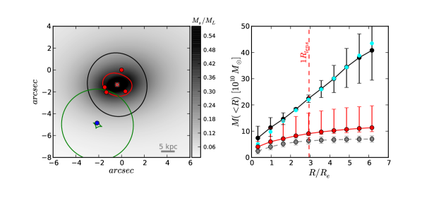
Figure 1: Comparison of two different modeling strategies on the lens PG1115+080. Left: A fit to a three-component lens model (stellar, dark matter, and external group) without population synthesis. Red dots mark the image positions and the red curve is the model critical curve. The blue dot is the model source position and the green curves show the model caustics. The grayscale indicates stellar-mass fraction, while the black ellipse indicates the ellipticity and position angle of the stellar component. The semi-major axis of the latter is arbitrary, and set here to $2R_{\textrm{\tiny{lens}}}$. Right: The red and cyan dots show the stellar and total enclosed mass respectively from the model in the left panel. The red error bars enclosing the red dots correspond to a $1\sigma$ region around the best $\chi^{2}$. The gray and black dots with error bars are the stellar mass and total enclosed mass respectively from the models in LFSF, which use pixellated lens models and population synthesis.

2 Multi-component fitting vs Stellar Population Modelling

The starting point of the present work is the models in LFSF of the projected stellar and total surface mass density from a sample of lensing galaxies. We obtained independent maps for the stellar mass and total mass, using archival data from the CASTLeS survey. The maps of stellar mass, $M_{\textrm{\tiny{stel}}}$, were derived by fitting stellar population synthesis models to photometry in two or more bands assuming a Chabrier (2003) initial mass function (IMF). The total or lens mass, $M_{\textrm{\tiny{lens}}}$, was mapped by computing pixellated lens models that fitted the lensed images and (where available) time delays. Detailed error estimates were derived in both cases. The enclosed total mass is well constrained at projected radii where images are present. At smaller and larger radii, $M_{\textrm{\tiny{lens}}}$ becomes progressively more uncertain. The outer radius of the mass maps is $2R_{\textrm{\tiny{lens}}}$ where $R_{\textrm{\tiny{lens}}}$ is the radius of the outermost image. Since $R_{\textrm{\tiny{lens}}}$ depends on the redshift and details of the source position, $2R_{\textrm{\tiny{lens}}}$ varies greatly among galaxies — from a quarter of the half-light radius ($R_{\textrm{\tiny{e}}}$) to several $R_{\textrm{\tiny{e}}}$.

Of the sample modelled in LFSF, 18 galaxies are early type systems. We exclude the Einstein Cross Q2237, which is the bulge of a spiral galaxy; B1600, which is likely to be a late-type galaxy viewed edge-on; and B1608, which is an ongoing merger. For these 18 early type galaxies, there is no evidence of a significant gaseous component, and hence we may assume that $\Delta M=M_{\textrm{\tiny{lens}}}-M_{\textrm{\tiny{stel}}}$ is a map of the dark matter distribution. The lensing maps tend to have similar orientation to the stellar mass, and hence the $\Delta M$ maps are fairly elliptical as well (Ferreras et al., 2008). In LFSF we obtained enclosed dark matter profiles $\Delta M(<R)$ using a circularized aperture along the elliptical isophotes, i.e. following the luminous distribution.

An alternative approach (see e.g. Auger et al., 2010; Trott et al., 2010) consists of fitting a parametric lens model with separate components for stellar and dark matter. If the stellar component can be correctly recovered by this method, the analysis based on stellar population synthesis constrained by multiband photometry will be dispensable. The two approaches are contrasted in Fig. 1 in the case of the quad PG1115+080. On the one hand we prepared separate models for $M_{\textrm{\tiny{lens}}}$ and $M_{\textrm{\tiny{stel}}}$ — a pixellated lens model for $M_{\textrm{\tiny{lens}}}$ and a stellar-population model from the photometry for $M_{\textrm{\tiny{stel}}}$. On the other hand, we fitted the lensing data to a multi-component parametric lens model: a de Vaucouleurs profile, plus an NFW halo, together with a singular isothermal sphere, adding external shear to account for a nearby galaxy group. We used the gravlens program (Keeton, 2001) together with Markov-chain Monte-Carlo (MCMC) to search for the best fit parameters. The effective radius was constrained to lie within the observational uncertainty $R_{\textrm{\tiny{e}}}=0.85\pm 0.07$ arcsec (Treu & Koopmans, 2002). The positions, ellipticities and position angle were also allowed to vary.

We see from Fig. 1 that the parametric and pixellated lens models give similar results for the total-mass profile. The pixellated method provides uncertainty estimates because it generates an ensemble of models. It is also computationally faster. However, the stellar mass is strongly overestimated by the parametric lens model, compared to the estimates based on population synthesis. In other words, the attempt to infer stellar masses from the lensing data alone fails. An explanation for this is suggested by the error bars on the total-mass. We see that lensing provides a good estimate of the enclosed mass at radii comparable to the images, but gets progressively more uncertain as we move inwards or outwards. Thus, attempting to extract the profile of a sub-component from this already-uncertain total-mass profile (without adding more data) will tend to amplify the errors.

Hence, for the rest of this paper, we will use the separate models of $M_{\textrm{\tiny{lens}}}$ and $M_{\textrm{\tiny{stel}}}$ from LFSF.

3 Virial mass and concentration

With the maps of $\Delta M=M_{\textrm{\tiny{lens}}}-M_{\textrm{\tiny{stel}}}$ surface mass density in hand, we now proceed to estimate a virial mass $M_{\textrm{\tiny{vir}}}$ and a concentration $c$ for each of the lensing galaxies. The method we adopt is to fit the profiles of $\Delta M(<R)$ to the cumulative projected mass of an NFW profile, which is given by:

$$M^{\textrm{\tiny{NFW}}}(<R)=4\pi\rho_{s}r_{s}^{3}\times\mathcal{F}(R,r_{s})$$ (1)

where

$$\mathcal{F}(r,r_{s})=\ln{\frac{r}{2r_{s}}}+\left\{\begin{array}[]{ll}\frac{1}{\sqrt{1-(\frac{r}{r_{s}})^{2}}}\cosh^{-1}\frac{r_{s}}{r}&(r<r_{s})\\ \stackrel{{\scriptstyle\phantom{-}}}{{1}}\phantom{\frac{1}{\sqrt{\frac{r}{r_{s}}^{2}}}}&(r=r_{s})\\ \frac{1}{\sqrt{(\frac{r}{r_{s}})^{2}-1}}\cos^{-1}\frac{r_{s}}{r}&(r>r_{s})\end{array}\right.$$ (2)

Here $r_{s}$ and $\rho_{s}$ are the scale radius and scale density parameters on which the NFW profile depends. For $\Delta M(<R)$ we assumed an error $\sigma=\sqrt{\delta_{M_{\textrm{\tiny{lens}}}}^{2}+\sigma_{M_{\textrm{\tiny{stel}}}}^{2}}$, where $\delta_{M_{\textrm{\tiny{lens}}}}$ is half of the $90\%$ confidence interval given by the ensemble of lens-mass models, and $\sigma_{M_{\textrm{\tiny{stel}}}}$ is the standard deviation of stellar mass from population synthesis. The best fit values of the parameters can be found in Table 2.

For two example lenses, Q0047-280 and HE2149-274, we illustrate the results in more detail in Figs. 2 and 3. The upper panels of Fig. 2 show parameter fits and $\chi^{2}$ contours. Note that the axes of these two panels are not simply $r_{s}$ and $\rho_{s}$ but rather $r_{s}/R_{e}$ and $\rho_{s}r_{s}^{2}$, in units of $M_{\odot}R_{\textrm{\tiny{e}}}^{-1}$. This choice tends to illustrate the parameters better. To check for the possibility of multiple local $\chi^{2}$-minima we generated MCMC chains with $10^{5}$ steps for each lens. Such additional minima can be excluded for physically interesting parameter values. As a further check, we compute as before the NFW parameters based on a $\chi^{2}$ search that best fit the steepest and shallowest profiles $M_{\textrm{\tiny{lens}}}(<R)$ allowed by the LFSF analysis of the lensing data. These are indicated by cyan crosses in Fig. 2 and, as expected, are roughly in the region of the fits to $\Delta M(<R)$.

The lower panels in Fig. 2 show parameter fits to the distributions of luminous matter, for the same two example galaxies, that we will use later, in Section 5. We use the well-known profile of Hernquist (1990). The enclosed projected form of the Hernquist (analogous to Eq. 1 for the NFW) is:

$$L(<R)=\frac{M}{\Upsilon}\left(\frac{R}{r_{h}}\right)^{2}\frac{\mathcal{X}(R,r_{h})-1}{1-\frac{R}{r_{h}}}$$ (3)

where

$$\mathcal{X}(r,r_{h})=\left\{\begin{array}[]{ll}\frac{1}{\sqrt{1-(r/r_{h})^{2}}}~{}\mathrm{sech}^{-1}(r/r_{h})&r\leq r_{h}\\ \frac{1}{\sqrt{(r/r_{h})^{2}-1}}~{}\mathrm{sec}^{-1}(r/r_{h})&r\geq r_{h}\end{array}\right.$$ (4)

Again, the parameters and $1\sigma$ errors as well as our values for $r_{\textrm{\tiny{vir}}}$ are given in Table 2. Note in the figure we show the contours with respect to total luminosity, i.e. $L\equiv M/\Upsilon$.

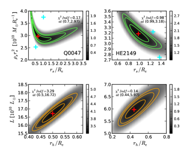
Figure 2: Parameter fits to dark matter and stellar ($\Delta M$ and $M_{\textrm{\tiny{stel}}}$) profiles for the lens galaxies B0047 and HE2149. Top: A $\chi^{2}$ map of the NFW parameter space for $\Delta M$, in grayscale with contours of $\Delta\chi^{2}=1,2,3$. Red crosses mark the overall best fit. Cyan crosses mark best fits to profiles at the steep and shallow ends of the confidence region. Bottom: The same for the Hernquist parameters for the luminosity $L$.

Figure 3 shows profiles of $\Delta M(<R)$, together with NFW fits and uncertainties. There is a tendency for the innermost point (in these two examples as well in other lenses in our study) to be higher than the fit. We note that various simulations (Moore et al., 1998; Navarro et al., 2004; Diemand et al., 2005) indicate a somewhat steeper slope than the original NFW. Recently Cardone et al. (2011) advocated a generalized NFW profile with an additional parameter. Furthermore, the presence of baryons will tend to steepen the central dark-matter profile through adiabatic contraction (although we note that feedback effects, such as baryon ejecta from supernovae-driven winds, or dynamical interactions with smaller structures could have the opposite effect, making the inner dark matter profile shallower). We will address the issue of adiabatic contraction later, in Section 4. For now we assume that a projected NFW depending on scale radius $r_{s}$ and the normalization $\rho_{s}$ sufficiently describe the data.

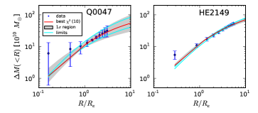
Figure 3: Inferred dark-matter profile $\Delta M$ and NFW fits, for the lens galaxies B0047 and HE2149. The red (cyan) line corresponds to the red (cyan) crosses in Figure 2.

¿From the NFW parameters $r_{s},\rho_{s}$ and given the redshift of the halo, the virial mass $M_{\textrm{\tiny{vir}}}$ and concentration $c$ are easily derived. Consider first the mass enclosed in a sphere (not to be confused with the cylindrical enclosed mass Eq. 1)

$$M_{\textrm{\tiny{sph}}}(<r)=4\pi\rho_{s}r_{s}^{3}\left\{\ln\left(1+\frac{r}{r_{s}}\right)-\frac{\frac{r}{r_{s}}}{1+\frac{r}{r_{s}}}\right\}$$ (5)

and the mean enclosed density within a given radius

$$\langle\rho(<r)\rangle=\frac{M_{\textrm{\tiny{sph}}}(<r)}{\frac{4}{3}\pi r^{3}}.$$ (6)

The virial radius is the $r$ at which the mean enclosed density equals a certain multiple $\Delta_{c}$ of the critical density, namely:

$$\langle\rho(<r_{\textrm{\tiny{vir}}})\rangle=\Delta_{c}\rho_{c}(z)$$ (7)

and the mass within the virial radius

$$M_{\textrm{\tiny{vir}}}=\Delta_{c}\rho_{c}(z)\times\frac{4}{3}\pi r_{\textrm{\tiny{vir}}}^{3}$$ (8)

is the virial mass. The concentration is defined as

$$c=\frac{r_{\textrm{\tiny{vir}}}}{r_{s}}.$$ (9)

The value for the overdensity is

$$\Delta_{c}=18\pi^{2}+82x-39x^{2}$$ (10)

where $x=(\Omega_{M}(1+z)^{3}/E(z)^{2})-1$ and $E(z)^{2}=\Omega_{M}(1+z)^{3}+\Omega_{\Lambda}$ (Bryan & Norman, 1998). This value of $\Delta_{c}$ gives the exact virial radius for a top-hat perturbation that has just virialized (see e.g. Peebles, 1980). The galaxies in our sample would have virialized well before the observed epoch. Hence, if the observed redshift is used to derive an $r_{\textrm{\tiny{vir}}}$, the value is unlikely to have the dynamical interpretation of a virial radius. Nevertheless, since such a definition of $r_{\textrm{\tiny{vir}}}$ is commonly adopted (e.g. Bryan & Norman, 1998; Buote et al., 2007) we adopt it in the present work.

The values of $c$ and $M_{\textrm{\tiny{vir}}}$, along with errors calculated according to the projected 1$\sigma$ regions of Figure 2, are quantities are listed in Table. 2. Figure 4 plots the values — there have been no previous data showing $M_{\textrm{\tiny{vir}}}$ vs $c$ to such small virial masses. For comparison, Figure 4 also shows the results from Buote et al. (2007) of the X-ray $c\,$-$M_{\textrm{\tiny{vir}}}$ relation for 39 systems. These range in $M_{\textrm{\tiny{vir}}}$ from $6\times 10^{12}$ to $2\times 10^{15}$ $M_{\odot}$. Buote et al. (2007) fit a power-law

$$c=\frac{c_{14}}{1+z}\left(\frac{M_{\textrm{\tiny{vir}}}}{M_{14}}\right)^{\alpha},$$ (11)

where $M_{14}=10^{14}h^{-1}M_{\odot}$ is a reference mass and $c_{14}$ and $\alpha$ are constants independent of $M$, obtaining $\alpha=-0.17\pm 0.03$. Leaving out the $(1+z)$-term gives $\alpha=-0.20\pm 0.03$. As in their analysis we use a bivariate fitting method for correlated errors and intrinsic scatter (BCES) due to Akritas & Bershady (1996), which gives $\alpha=-0.40\pm 0.06$.

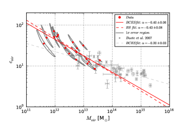
Figure 4: Concentration versus virial mass. The red dots represent data from this study. The grey circles shows data from Buote et al. (2007). The grey contours show the $1\sigma$ error region from Fig. 1. The red dashed line shows a bootstrapping fit to our data. The solid red line shows the result of a bivariate fitting method for correlated errors and instrinsic scatter (BCES) by Akritas & Bershady (1996) applied to the data. The same method was used by Buote et al. (2007) to obtain the dashed grey line.

Note how in Figure 4 the projected $1\sigma$ contours cover a smaller region than simple vertical and horizontal error bars would imply. This suggests that more information might be available with the appropriate tools. Hence, we tried alternative fitting approaches. In a parametric boostrap we randomly resample over arbitrary points within the $1\sigma$ contours, so that one point per lens is used for an ordinary least square fit. This is done for $10^{4}$ realizations. In a later run we ease the requirement of one point per lens and pick instead a number $n<18$ out of the total number of lenses to perform the resampling. In all cases the mean value of the slope $\alpha$ stays the same, but its distribution gets broader for smaller values of $n$. For $n=18$ the bootstrapping analysis yields $\alpha=-0.42\pm 0.08$. We also employed a piecewise analysis to check how the slope $\alpha$ of the relation evolves and to see whether fits in common mass range yield similar results. Furthermore we fit a combined sample of 57 objects. The results are shown in Table 1.

Going from high to low $M_{\textrm{\tiny{vir}}}$ the slope increases from $-0.10\pm 0.05$ for $M_{\textrm{\tiny{vir}}}>10^{14}M_{\odot}$ to $-0.20\pm 0.13$ for $M_{\textrm{\tiny{vir}}}<10^{14}M_{\odot}$ (Buote et al., 2007) and finally $-0.40\pm 0.06$ for $M_{\textrm{\tiny{vir}}}<4\times 10^{13}$. For the mass range between $6\times 10^{12}$ $M_{\odot}$ and $1\times 10^{14}$ $M_{\odot}$, where the two samples overlap, we do not find significant differences — a two-dimensional Kolmogorov-Smirnov test for the overlapping region gives a $p$-value of $\sim 0.5$ under the null hypothesis that both samples are drawn from the same population. However, it should be noted that the reduced sample size and considerable scatter leads to large errors for both samples. A trend of $\alpha$ with virial mass was first suggested by Navarro et al. (1996) and confirmed by Bullock et al. (2001) and Eke et al. (2001) for simulations. Higher normalization factors compared to simulations are also known from a lensing study by Comerford & Natarajan (2007).

Sample	Size	Method	$M_{\textrm{\tiny{vir}}}$-range	$\alpha$	$c_{14}$
			[$10^{14}M_{\odot}$]
B07	39	BCES	$0.06-20$	$-0.199\pm 0.026$	$9.12\pm 0.43$
B07	22	BCES	$>1$	$-0.103\pm 0.055$	$7.71\pm 0.58$
B07	17	BCES	$<1$	$-0.201\pm 0.129$	$9.46\pm 2.11$
$c$	18	BCES	$0.004-0.4$	$-0.401\pm 0.064$	$7.03\pm 1.49$
$c$	18	BS	$0.004-0.4$	$-0.433\pm 0.078$	$6.60^{+33.1}_{-6.2}$
$c$	9	BCES	$>0.06$	$-0.203\pm 0.172$	$16.98\pm 12.87$
comb	57	BCES	$0.004-20$	$-0.278\pm 0.021$	$9.62\pm 0.41$
B070	39	BCES	$0.06-20$	$-0.172\pm 0.026$	$9.0\pm 0.4$
$c_{vir,0}$	18	BCES	$0.004-0.4$	$-0.381\pm 0.062$	$12.02\pm 2.57$
CN70	62	N/K	$0.4-100$	$-0.15\pm 0.13$	$10.68\pm 5.50$

Table 1: Slope $\alpha$ of the $c-M_{\textrm{\tiny{vir}}}$ relation with uncertainty for different samples, sample sizes, fitting methods and mass ranges (all errors $1\sigma$, $c_{14}$ errors for BS-method are $68\%$ conf. interterval around median). B07 denotes the sample of massive early types in Buote et al. (2007), $c$ stands for the relation as in Fig. 4, $comb$ gives the combined sample fit consisting of 39 objects of B07 and 18 lenses of the above $cvir$ sample, CN7 are results from Comerford & Natarajan (2007). The index $0$ to a sample name denotes concentrations normalized to $z=0$.

4 Comparison with abundance matching

Thus far we have computed $c$ and $M_{\textrm{\tiny{vir}}}$ under the assumptions that (a) an NFW profile is a good representation of the dark matter profile beyond the radial range probed for lens galaxies in LFSF, and (b) the dark matter profile is well constrained by pixellated studies of stellar and total mass, meaning also that the probed radial range is sensitive to the scale radius of the NFW profile and that the uncertainties give a robust estimate of the suitable mass distributions. We now compare the quantities extrapolated to the virial radius with predictions using both simulations and SDSS observations.

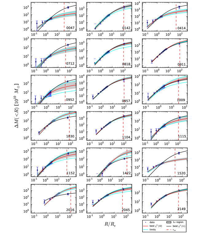
Figure 5: Extension of Fig. 3 to the virial radius and for the whole lens sample. In each panel there are three additional elements not present in Fig. 3: the vertical dashed line marks the the $r_{\textrm{\tiny{vir}}}$ inferred from the NFW fit; the outer isolated point shows the virial radius and virial mass inferred from abundance matching; the black curve is an NFW fit constrained to go through the abundance-matching point.

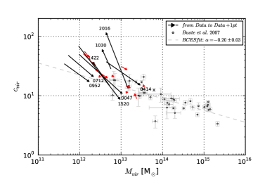
Figure 6: Similar to Fig. 4, but showing how the fits change when abundance matching is included. The arrows go from the original position (red dots in Fig. 4) to the position for which the parameters include information on virial mass from Moster et al. (2010). The red arrows mark the 10 lenses for which the extrapolated NFW analysis and abundance matching give consistent answers.

Abundance matching studies like Moster et al. (2010) and Guo et al. (2010) make use of cosmological simulations and galaxy surveys to determine the mass dependence of galaxies and their preferred host haloes. The stellar mass enclosed within a $2R_{\textrm{\tiny{lens}}}$ aperture is known from our population synthesis modelling, as shown in LFSF. The stellar mass profiles do not change significantly beyond $2R_{\textrm{\tiny{lens}}}$. Thus we use the $M_{\textrm{\tiny{halo}}}$-to-$M_{\textrm{\tiny{stel}}}$ relation from Moster et al. (2010) to infer a virial mass and the corresponding scatter (taken at the $1\sigma$ level). Note that the above abundance matching relations are based on Kroupa/Chabrier IMFs and thus consistent with the stellar masses used here. Fig. 5 shows the extrapolation of the NFW fits out to the virial radius. The figure also adds an extra point $(r_{\textrm{\tiny{vir}}}^{\textrm{\tiny{AM}}},M_{\textrm{\tiny{vir}}}^{\textrm{\tiny{AM}}})$ marking the virial radius and mass from abundance matching. For 10 out of the 18 lenses, $M_{\textrm{\tiny{vir}}}^{\textrm{\tiny{AM}}}$ turns out to lie within the $1\sigma$ confidence region (grey shaded) around the original fit for $\Delta M(R)$. Accordingly, we show a further NFW fit (black curve) that is constrained to pass through $(r_{\textrm{\tiny{vir}}}^{\textrm{\tiny{AM}}},M_{\textrm{\tiny{vir}}}^{\textrm{\tiny{AM}}})$.

In Fig. 6 we show how the $c$-$M_{\textrm{\tiny{vir}}}$ scatter plot changes when we impose abundance matching. The arrows point from values without the abundance-matching information to values including it, and the longer arrows are labelled. Going from Fig. 4 to Fig. 6 leads mostly to shifts along the direction of the relation, but the rms scatter with respect to the simple power-law fit almost doubles, from 0.145 to 0.258. In comparison, the Buote et al. (2007) sample has a rms scatter of 0.180. A mildly increased scatter can be found in simulations by Shaw et al. (2006) for virial masses between $\sim 3\times 10^{13}$ and $\sim 10^{15}M_{\odot}$, which is most likely due to the indistinguishability between substructure and main haloes. However, this cannot explain the increased scatter we find. We can conclude that the extrapolation to $r_{\textrm{\tiny{vir}}}$ inferred in Section 3 gives a reasonable extension to the $c$-$M_{\textrm{\tiny{vir}}}$ relation. Abundance matching, on the other hand, appears to introduce a large discrepancy in some cases. Three of the galaxies (MG2016, B1422 and B1030) show a shift to a much higher concentration when abundance matching is imposed. These are lenses for which $M_{\textrm{\tiny{vir}}}^{\textrm{\tiny{AM}}}$ lies significantly below the extrapolation $M_{\textrm{\tiny{vir}}}$. For MG2016, $M_{\textrm{\tiny{vir}}}^{\textrm{\tiny{AM}}}$ is even smaller than $\Delta M(<R)$ at the outermost radius of the lens model. Further three galaxies (Q0047, MG0414, SBS1520) show large shifts towards lower concentrations. They belong to the highest redshift galaxies in our sample and are probed in an exceptionally large radial range, up to $10\%$ of the virial radius (see column $2R_{\textrm{\tiny{lens}}}/r_{\textrm{\tiny{vir}}}$ in Tab. 2). Moreover, MG2016 and SBS1520, which exhibit strongly discrepant $M_{\textrm{\tiny{vir}}}^{\textrm{\tiny{AM}}}$, have reconstructed mass profiles with comparatively small uncertainties.

So what is the reason for this discrepancy? A possible explanation is suggested by a visible correlation between the length of the arrows and the environment of the lenses. For extrapolated virial masses much lower than $M_{\textrm{\tiny{vir}}}^{\textrm{\tiny{AM}}}$ one may argue that lens profiles are shallower in group or cluster environments than in more isolated locations. This reflects the inverse proportionality of concentration and enclosed mass and is a consequence of hierarchical structure formation. Extrapolating mass profiles from shallower profiles leads necessarily to lower masses at $r_{\textrm{\tiny{vir}}}$. In other words, if the $M_{\textrm{\tiny{halo}}}(M_{\textrm{\tiny{stel}}})$ obtained from abundance matching is employed to determine $M_{\textrm{\tiny{vir}}}^{\textrm{\tiny{AM}}}$, we implicitly assume an isolated galaxy located within a ”typical” halo with respect to its stellar content and the halo definition used in the abundance matching procedure. For lenses with extrapolated virial masses much larger than $M_{\textrm{\tiny{vir}}}^{\textrm{\tiny{AM}}}$ the mere effect of the projected cluster environment might become more important, that is, although being relatively shallow, the projected total mass profile is strongly influenced by dark matter in the cluster acting as an additional convergence. This again causes the extrapolation to be significantly different from $M_{\textrm{\tiny{vir}}}^{\textrm{\tiny{AM}}}$. Examples for the latter case are MG2016 and B1422, which are located in the densest environments among our lenses with large groups or clusters showing many nearby galaxies (cf. Table 1 in LFSF).

All 8 lenses for which $M_{\textrm{\tiny{vir}}}^{\textrm{\tiny{AM}}}$ is strongly discrepant with $M_{\textrm{\tiny{vir}}}$ are in dense environments, whereas for 6 out of 10 remaining galaxies, there are no nearby objects reported so far. Current abundance-matching prescriptions do not consider environmental effects. Our results suggest that environment may significantly influence the $M_{\textrm{\tiny{halo}}}(M_{\textrm{\tiny{stel}}})$ function.

5 Adiabatic contraction

In the following section we will assess the extent to which the $c\,$-$M_{\textrm{\tiny{vir}}}$ relation could be caused by adiabatic contraction of the halo. Blumenthal et al. (1986) proposed that during the formation of galaxy-sized structures, the collapse of the dissipative baryons towards the centre of the forming halo would extert a reaction on the dark matter density profile, making it steeper. This effect would mean that simple N-body simulations, such as those that led to the proposal of the NFW profile (Navarro et al., 1996), would underestimate the inner slope of the halo.

The concentrations derived in Section 3 would therefore represent the state of the halo after adiabatic contraction (AC). In this Section, we will refer to these concentrations as $c_{\textrm{\tiny{final}}}$. Before AC, the concentrations are thought to have a lower value $c_{\textrm{\tiny{init}}}$. At present it is not clear whether or not $c_{\textrm{\tiny{init}}}$ differed from $c_{\textrm{\tiny{final}}}$ (e.g., Abadi et al., 2010) and it is conceivable that the impact of AC on dark matter profiles might be overestimated by commonly used recipes for baryonic cooling. Additional mechanisms such as dynamical encounters with smaller structures (see e.g. El-Zant et al., 2004; Cole et al., 2011), or the ejecta of baryons triggered by supernovae-driven winds (Larson, 1974; Dekel & Silk, 1986; Brooks et al., 2007) could lead to the opposite effect, making the inner slope of the dark matter profile less cuspy. In this paper we only consider the effect from the more fundamental process of contraction during the formation of the halo.

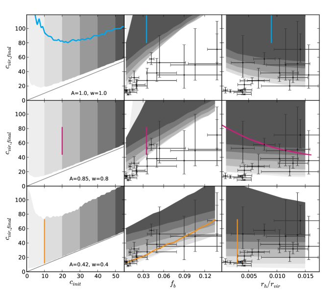
Figure 7: Adiabatic contraction following Gnedin et al. (2004). Each row corresponds to a different set of values for the parameters $A$ and $w$ in Equation (12). Each row shows the final concentration against: (left) the initial concentration, (middle) the baryon fraction, and (right) the scale radius of the baryons. The initial concentration can be read off the middle and right panels by comparing the gray bands with the left panel of the same row. The colored lines illustrate the effect of holding fixed two out of (i) initial concentration, (ii) baryon faction and (iii) baryon scale radius.

5.1 Comparing Adiabatic Contraction Models

To analyze this issue, we make use of the halo contraction program of Gnedin et al. (2004), which computes the change in the dark-matter density profile under AC, keeping $rM(<r)$ conserved. To take account of a wide range of orbit eccentricities the code invokes the power-law

$$\bar{r}/r_{\textrm{\tiny{vir}}}=A(r/r_{\textrm{\tiny{vir}}})^{w}$$ (12)

to describe the mean relation between orbit-averaged and current radius, and modifies the adiabatic invariant to $rM(<\bar{r})$. Eq. 12 changes the eccentricity distribution of the mass profile, which is thus distorted by the usage of a mean radius in the invariant. Parameter $A$ defines the maximum eccentricity and causes $rM(<\bar{r})$ to be larger than $rM(<r)$ for $r/r_{\textrm{\tiny{vir}}}<0.44$ and smaller for $r/r_{\textrm{\tiny{vir}}}>0.44$. A larger invariant means more mass in the center at the expense of the outer parts of the halo. The parameter $w$ defines how strong the shift is. The smaller $w$ the fewer mass at the center.

The case $A=w=1$ therefore corresponds to the original prescription of Blumenthal et al. (1986), where the orbits are assumed to be completely circular. This case can be understood as an upper limit to AC. The program provides the necessary resolution for comparison with our data, i.e., down to $10^{-3}r_{\textrm{\tiny{vir}}}$. The input parameters are $f_{b}$, the baryon fraction enclosed within $r_{\textrm{\tiny{vir}}}$, the baryon scale length and the initial concentration of the dark matter halo, $c_{\textrm{\tiny{init}}}$. We take the baryon fraction as $M_{\textrm{\tiny{stel}}}(<2R_{\textrm{\tiny{lens}}})/M_{\textrm{\tiny{vir}}}$, where $M_{\textrm{\tiny{stel}}}(<2R_{\textrm{\tiny{lens}}})$ denotes the stellar mass enclosed in the total reconstructed radial range. For the baryon scale length we use the fitted Hernquist scale radius $r_{h}$ derived in Section 3. This is preferred to making use of $R_{\textrm{\tiny{e}}}\approx r_{h}\times 1.8$ (Hernquist, 1990), because our measured $R_{\textrm{\tiny{e}}}$ – derived from the Petrosian radius – do not agree precisely with the half-light radius of Hernquist profiles, which is a consequence of projected radii and circularized mass profiles. Furthermore, the Hernquist profile is originally used for the surface brightness distribution, whereas we fit in this case surface mass profiles. The $r_{h}/R_{\textrm{\tiny{e}}}$ best-fit values turn out to be mostly lower but close to $1/1.8$.

We run the contraction routine for a grid of parameters $(c_{\textrm{\tiny{init}}},f_{b},r_{h}/r_{\textrm{\tiny{vir}}})$ ranging from $(5,0.005,0.001)$ to $(60,0.135,0.015)$ in steps of $(1,0.01,0.002)$. We then fitted the contracted profiles, via Eq. 5 to the data $\Delta M(<R)$ for $R/r_{\textrm{\tiny{vir}}}$ ranging from $\sim 0.006$ to $0.12$.

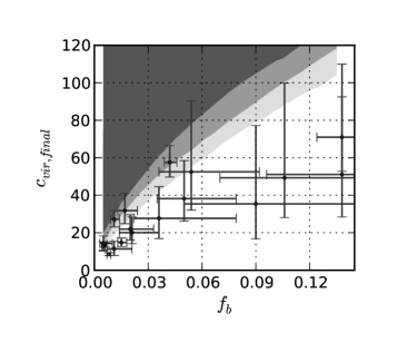
Figure 8: Final concentration versus baryon fraction depending on size of radial window for the AC prescription of Gnedin et al. (2004). Bright to dark grey corresponds to aperture sizes $(\sim 0.003-0.06)r_{\textrm{\tiny{vir}}}$ ,$(\sim 0.005-0.09)r_{\textrm{\tiny{vir}}}$ and $(\sim 0.006-0.12)r_{\textrm{\tiny{vir}}}$.

There are a number of uncertainties entering the analysis:

1. since the radial extent of a reconstructed profile is limited to 2 times the angular $R_{\textrm{\tiny{lens}}}$ and a finite resolution, the aperture size changes from lens to lens,

2. in order to mimic the limited probed range (henceforth called aperture) by an equivalent range in the contracted profile, $R_{\textrm{\tiny{lens}}}$ must be expressed in units of $r_{\textrm{\tiny{vir}}}$,

3. baryon fraction as well as baryonic scale length depend on $M_{\textrm{\tiny{vir}}}$ and $r_{\textrm{\tiny{vir}}}$ which are extrapolated quantities with their respective uncertainties.

Figure 7 shows the results for three scenarios of adiabatic contraction. The leftmost panels show initial versus final (i.e. contracted) halo concentration. The top row corresponds to the original proposal of Blumenthal et al. (1986) ($A=1.0$, $w=1.0$, i.e., no correction for anisotropic orbits). In this case, we illustrate the increase in concentration as a blue line for fixed values of $f_{b}$ and $r_{h}/r_{\textrm{\tiny{vir}}}$. The growing concentration towards low $c_{\textrm{\tiny{init}}}$ is a consequence of the interplay between radial aperture – i.e. the extent of the extrapolation – and the region affected by AC. The smaller the initial concentration the larger $c_{\textrm{\tiny{final}}}/c_{\textrm{\tiny{init}}}$ towards small radii for the same $f_{b}$ (we refer to this as the AC-sensitive case.). As $c_{\textrm{\tiny{init}}}$ increases the difference between final and initial profile subsides. Note that in our analysis, the further out we can probe the halo, the less affected is the fit and the extrapolation. However, for different combinations of $f_{b}$ and $r_{h}/r_{\textrm{\tiny{vir}}}$, similar curves fill the grey-shaded region. To enable proper differentiation with respect to initial concentration, we choose different shades of gray. The middle (rightmost) panels show the final concentration versus baryon fraction (baryon-to-virial radius fraction). The gray shaded regions map the same areas as those in the leftmost panels. The black dots with error bars represent our data. For the Blumenthal et al. (1986) case (top), there is clearly a disagreement between observationally inferred and contracted profiles. Especially the low-$f_{b}$ and low-$r_{h}/r_{\textrm{\tiny{vir}}}$ regions show significant departure from even the lowest final concentrations of the generic haloes. The middle row of Figure 7 shows the AC prescription of Gnedin et al. (2004), that implements eq. 12 with fiducial values $A=0.85$ and $w=0.8$ to take into account eccentric orbits. This phenomenologically motivated ansatz leads to smaller concentrations. There is still significant disagreement between data and simulated contraction. The behavior of $c_{vir,final}$ as a function of $r_{h}/r_{\textrm{\tiny{vir}}}$ for constant $c_{vir,final}$ and $f_{b}$ is indicated by the solid magenta line. For the panels in the bottom row of Fig. 7, we changed the pre-defined values of $A$ and $w$ to 0.42 and 0.4, respectively. The orange line shows for fixed $c_{\textrm{\tiny{init}}}$ and $r_{h}/r_{\textrm{\tiny{vir}}}$ the final concentration as a function of $f_{b}$. These values for $A$ and $w$ give good agreement with the lensing data even for low $c_{\textrm{\tiny{init}}}$, between 1 and 10. Compared to the AC prescriptions shown in the top and middle rows, the range of final concentrations is narrower, corresponding to a shallower $c_{\textrm{\tiny{final}}}$-$f_{b}$ relation (middle panels). The latter can be equivalently expressed in terms of mass not drawn into the central region $<0.1r_{\textrm{\tiny{vir}}}$. Comparing mass profiles contracted according to Gnedin et al. (2004) with the $(A=0.42,w=0.4)$-case shows that the latter transports less mass ($\sim 0.4\%$ of the virial mass) into the central halo region, $<0.1r_{\textrm{\tiny{vir}}}$.

One of the intriguing results of this study is that even with a simple assumption of a common, mass-independent initial concentration, most of the final concentrations can be explained if ($A$,$w$) are conveniently adjusted and $r_{h}$ is allowed to vary within uncertainties. There are a variety of results we summarize in the following.

• There is slight evidence for lenses with lower baryon fraction to require higher initial concentrations.

• Both smaller $c_{\textrm{\tiny{init}}}$ and smaller $r_{h}/r_{\textrm{\tiny{vir}}}$ produce steeper $c_{\textrm{\tiny{final}}}(f_{b})$ curves. This effect is independent of the AC-sensitive case at very low $c_{\textrm{\tiny{init}}}$ (explained above).

• When $A$ and $w$ are reduced, $c_{\textrm{\tiny{final}}}(f_{b})$ and $c_{\textrm{\tiny{final}}}(r_{h})$ become flatter, i.e. the differently shaded $c_{\textrm{\tiny{init}}}$ regions of the leftmost panels are mapped to narrower regions in the middle and right panels. Moreover their overlap is reduced.

To study how sensitive our results are to the radial range, we additionally provide in Fig. 8 the results for reduced aperture sizes, i.e. $(\sim 0.005-0.09)r_{\textrm{\tiny{vir}}}$ and $(\sim 0.003-0.06)r_{\textrm{\tiny{vir}}}$ using the parameters $A=0.85$ and $w=0.8$. We find that even for the smallest radial range fits do not yield agreement with our lens data. The case that we underestimate the radial extend of our lenses by a factor of two is in light of the relatively small uncertainties of the mass profiles and the errors attached to $r_{s}$ unlikely. Larger radial apertures yield even more disfavored final concentrations compared to our lens data.

5.2 Initial Concentration from Weak Adiabatic Contraction

For the weak AC case $(A=0.42,w=0.4)$ we compare the number of different ($c_{\textrm{\tiny{init}}}$,$r_{h}/r_{\textrm{\tiny{vir}}}$) combinations producing final concentrations in agreement with our lens data and infer a $c_{\textrm{\tiny{init}}}$-$M_{\textrm{\tiny{vir}}}$ plot as before, enriched by the information of the frequency distribution of initial concentrations (see Fig. 9). Although most of the data can be reproduced even by few initial concentrations of $\sim 1$, most of the ($c_{\textrm{\tiny{init}}}$,$r_{h}/r_{\textrm{\tiny{vir}}}$) combinations with high $c_{\textrm{\tiny{init}}}$ produce final concentration in agreement with $c_{\textrm{\tiny{final}}}$ and $f_{b}$. The hue of the magenta column indicates the frequency distribution of $c_{\textrm{\tiny{init}}}$ values whereas the $68\%$ ($99\%$) confidence interval is highlighted by strongest (faintest) color.

Certainly, no strong quantitative conclusions can yet be drawn from these results, but judging by the confidence regions a strongly flattened $c_{\textrm{\tiny{init}}}(M_{\textrm{\tiny{vir}}})$ relation seems likely. These results are in agreement with the inital halo concentrations estimated by Lintott et al. (2006), who used a simple model of spherical collapse. In that model, massive galaxies from density fluctuations between 2 and 3$\sigma$ – roughly mapping the same mass range as our lensing galaxies – were found with initial concentrations between 3 and 10, with the most massive ones having lower concentrations. A flattened low-mass end of the $c-M_{\textrm{\tiny{vir}}}$ relation is expected by simulations. To show this we include results from Macciò et al. (2007) (solid line and grey $2\sigma$ band in Fig. 9). $c(M,z)$ curves based on a toy model by Bullock et al. (2001) for redshifts in a range from 0 to 1.4 are in good agreement with results from N-body simulations. The toy model includes the free parameter $K$ which takes into account the contraction of the inner halo beyond that required by the top-hat formation scenario. This contraction parameter is fixed for all haloes in their simulation. The difference between the simulated and observed $c-M_{\textrm{\tiny{vir}}}$ relation is a well-known issue and matter of ongoing studies. It is however worthwhile to mention that this discrepancy is even stronger for low virial mass. From the comparison between $c_{\textrm{\tiny{init}}}$-$M_{\textrm{\tiny{vir}}}$ found in this study and simulations that investigate the redshift-dependence, we can conclude that Adiabatic Contraction alone is not enough to explain the slope of the relation.

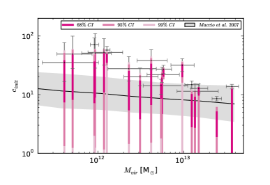
Figure 9: As in Fig. 4, but with initial concentrations. The colors of the columns from dark to bright correspond to the $68\%$, $95\%$ and $99\%$ confidence intervals of a range of ($c$,$f_{b}$,$r_{h}/r_{\textrm{\tiny{vir}}}$) values which produce a $c_{\textrm{\tiny{final}}}$ in agreement with our data. For comparison we include $c_{\textrm{\tiny{final}}}(M_{\textrm{\tiny{vir}}})$ and results from simulations by Macciò et al. (2007). The solid line indicates their mean concentration together with a $2\sigma$ band (grey region).

6 Conclusions

Strong gravitational lensing on galaxy scales constitutes a powerful tool to characterize dark matter haloes. In addition, combining photometric studies with stellar population synthesis allows us to assess the interplay between baryons and dark matter in the central regions of galaxies. This paper extends the work of LFSF by exploring in detail the concentration of the dark matter haloes of 18 massive early-type lensing galaxies. On a concentration-virial mass diagram (Fig. 4) we find these haloes to confirm and extend towards lower masses the relationship observed in X-rays by Buote et al. (2007).

Our sample includes information about the baryon fraction, enabling us to explore the validity of adiabatic contraction prescriptions, such as the one of Blumenthal et al. (1986) or Gnedin et al. (2004). We find that the standard modelling gives rather high final concentrations compared to our observations (Fig. 7). A tweak of the parameters in the AC prescription of Gnedin et al. (2004) cause the gain in mass of the central region ($<0.1r_{\textrm{\tiny{vir}}}$) to be $\sim 4\times 10^{-3}M_{\textrm{\tiny{vir}}}$ lower than in the previous case, which helps to solve the discrepancy. Furthermore, this results in a rather flat relationship between initial concentration (i.e. pre-AC) and halo.

We emphasize that this paper focusses on the fundamental aspect of adiabatic contraction caused by the collapse of the baryons during the formation of the haloes. Additional mechanisms acting later, arising from dynamical interactions (El-Zant et al., 2004; Cole et al., 2011) or stellar feedback resulting in the expulsion of baryons (see e.g. Read & Gilmore, 2005; Brooks et al., 2007) may alter the inner slope of the dark matter halo, although these mechanisms are expected to be more important in lower mass galaxies. Nevertheless, the tweak in the AC prescription of Gnedin et al. (2004) could be interpreted as one of these mechanisms playing a role in the evolution of the structure of the haloes. In any case, our analysis suggests that adiabatic contraction can explain only part of the $c$-$M_{\textrm{\tiny{vir}}}$ trend but is unlikely to be the sole origin of it.

References

- Abadi et al. (2010) Abadi, M. G., Navarro, J. F., Fardal, M., Babul, A., & Steinmetz, M. 2010, MNRAS, 407, 435
- Auger et al. (2010) Auger M. W., Treu T., Bolton A. S., Gavazzi R., Koopmans L. V. E., Marshall P. J., Moustakas L. A., Burles S., 2010, ApJ, 724, 511
- Akritas & Bershady (1996) Akritas, M. G. & Bershady, M. A. 1996, ApJ, 470, 706
- Blumenthal et al. (1986) Blumenthal, G. R., Faber, S. M., Flores, R. & Primack, J. R. 1986, ApJ, 301, 27
- Brooks et al. (2007) Brooks A. M., Governato F., Booth C. M., Willman B., Gardner J. P., Wadsley J., Stinson G., Quinn T., 2007, ApJ, 655, L17
- Bryan & Norman (1998) Bryan, G. L. & Norman, M. L. 1998, ApJ, 495, 80
- Bullock et al. (2001) Bullock, J. S., Kolatt, T. S., Sigad, Y., Somerville, R. S., Kravtsov, A. V., Klypin, A. A., Primack, J. R., & Dekel, A. 2001, MNRAS, 321, 559
- Buote et al. (2007) Buote, D. A., Gastaldello, F., Humphrey, P. J., Zappacosta, L., Bullock, J. S., Brighenti, F., & Mathews, W. G. 2007, ApJ, 664, 123
- Cappellari et al. (2006) Cappellari, M., et al. 2006, MNRAS, 366, 1126
- Cardone et al. (2011) Cardone, V. F., Del Popolo, A., Tortora, C., & Napolitano, N. R. 2011, MNRAS, 416, 1822
- Chabrier (2003) Chabrier G., 2003, PASP, 115, 763
- Coccato et al. (2009) Coccato L., et al., 2009, MNRAS, 394, 1249
- Cole et al. (2011) Cole, D. R., Dehnen, W. & Wilkinson, M. I. 2011, MNRAS, 416, 1118
- Comerford & Natarajan (2007) Comerford, J. M. & Natarajan, P. 2007, MNRAS, 379, 190
- Côté et al. (2001) Côté P., McLaughlin D. E., Hanes D. A., Bridges T. J., Geisler D., Merritt D., Hesser J. E., Harris G. L. H., Lee M. G., 2001, ApJ, 559, 828
- Deason et al. (2011) Deason A. J., Belokurov V., Evans N. W., McCarthy I. G., 2011, ApJ, in press (arxiv:1110.0833)
- Dekel & Silk (1986) Dekel A., Silk J., 1986, ApJ, 303, 39
- de Lorenzi et al. (2009) de Lorenzi F., et al., 2009, MNRAS, 395, 76
- Diemand et al. (2005) Diemand, J., Zemp, M., Moore, B., Stadel, J., & Carollo, C. M. 2005, MNRAS, 364, 665
- Douglas et al. (2002) Douglas, N. G., et al. 2002, PASP, 114, 1234
- Eke et al. (2001) Eke, V. R., Navarro, J. F., & Steinmetz, M. 2001, ApJ, 554, 114
- El-Zant et al. (2004) El-Zant, A. A., Hoffman, Y., Primack, J., Combes, F. & Shlosman, I. 2004, ApJ, 607, L75
- Ferreras et al. (2008) Ferreras, I., Saha, P., & Burles, S. 2008, MNRAS, 383, 857
- Gerhard et al. (2001) Gerhard O., Kronawitter A., Saglia R. P., Bender R., 2001, AJ, 121, 1936
- Gnedin et al. (2004) Gnedin, O. Y., Kravtsov, A. V., Klypin, A. A., & Nagai, D. 2004, ApJ, 616, 16
- Guo et al. (2010) Guo, Q., White, S., Li, C., & Boylan-Kolchin, M. 2010, MNRAS, 367
- Hernquist (1990) Hernquist, L. 1990, ApJ, 356, 359
- Hui et al. (1995) Hui X., Ford H. C., Freeman K. C., Dopita M. A., 1995, ApJ, 449, 592
- Keeton (2001) Keeton, C. R. 2001, arXiv:astro-ph/0102340
- Larson (1974) Larson R. B., 1974, MNRAS, 169, 229
- Leier et al. (2011) Leier D., Ferreras I., Saha P., Falco E. E., 2011, ApJ, 740, 97
- Lintott et al. (2006) Lintott, C. J., Ferreras, I. & Lahav, O. 2006, ApJ, 648, 826
- Macciò et al. (2007) Macciò, A. V., Dutton, A. A., van den Bosch, F. C., Moore, B., Potter, D., Stadel, J. 2007, MNRAS, 378, 55
- Moore et al. (1998) Moore, B., Governato, F., Quinn, T., Stadel, J., & Lake, G. 1998, ApJ, 499, L5
- Moster et al. (2010) Moster, B. P., Somerville, R. S., Maulbetsch, C., van den Bosch, F. C., Macciò, A. V., Naab, T., & Oser, L. 2010, ApJ, 710, 903
- Napolitano et al. (2009) Napolitano, N. R., et al. 2009, MNRAS, 393, 329
- Navarro et al. (1996) Navarro, J. F., Frenk, C. S., & White, S. D. M. 1996, ApJ, 462, 563
- Navarro et al. (2004) Navarro, J. F., Hayashi, E., Power, C., Jenkins, A. R., Frenk, C. S., White, S. D. M., Springel, V., Stadel, J., & Quinn, T. R. 2004, MNRAS, 349, 1039
- Neto et al. (2007) Neto, A. F., et al., 2007, MNRAS, 381, 1450
- Peebles (1980) Peebles, P. J. E. 1980, The large scale structure of the Universe, Princeton University Press
- Read & Gilmore (2005) Read, J. I. & Gilmore, G., 2005, MNRAS, 356, 107
- Romanowsky et al. (2003) Romanowsky, A. J., Douglas, N. G., Arnaboldi, M., Kuijken, K., Merrifield, M. R., Napolitano, N. R., Capaccioli, M., Freeman, K. C. 2003, Science, 301, 1696
- Romanowsky et al. (2009) Romanowsky A. J., Strader J., Spitler L. R., Johnson R., Brodie J. P., Forbes D. A., Ponman T., 2009, AJ, 137, 4956
- Sato et al. (2000) Sato S., Akimoto F., Furuzawa A., Tawara Y., Watanabe M., Kumai Y., 2000, ApJ, 537, L73
- Schuberth et al. (2010) Schuberth, Y., Richtler, T., Hilker, M., Dirsch, B., Bassino, L. P., Romanowsky, A. J., Infante, L. 2010, A& A, 513, 52
- Shaw et al. (2006) Shaw, L. D., Weller, J., Ostriker, J. P., & Bode, P. 2006, ApJ, 646, 815
- Thomas et al. (2009) Thomas J., Saglia R. P., Bender R., Thomas D., Gebhardt K., Magorrian J., Corsini E. M., Wegner G., 2009, ApJ, 691, 770
- Treu & Koopmans (2002) Treu, T. & Koopmans, L. V. E. 2002, MNRAS, 337, L6
- Trott et al. (2010) Trott C. M., Treu T., Koopmans L. V. E., Webster R. L., 2010, MNRAS, 401, 1540