Precision Thrust Cumulant Moments at N³LL

Abstract

We consider cumulant moments (cumulants) of the thrust distribution using predictions of the full spectrum for thrust including ${\cal O}(\alpha_{s}^{3})$ fixed order results, resummation of singular N³LL logarithmic contributions, and a class of leading power corrections in a renormalon-free scheme. From a global fit to the first thrust moment we extract the strong coupling and the leading power correction matrix element $\Omega_{1}$. We obtain $\alpha_{s}(m_{Z})=0.1140\,\pm\,(0.0004)_{\rm exp}\,\pm\,(0.0013)_{\rm hadr}\,\pm\,(0.0007)_{\rm pert}$, where the $1$-$\sigma$ uncertainties are experimental, from hadronization (related to $\Omega_{1}$) and perturbative, respectively, and $\Omega_{1}=0.377\,\pm\,(0.044)_{\rm exp}\,\pm\,(0.039)_{\rm pert}\,{\rm GeV}$. The $n$-th thrust cumulants for $n\geq 2$ are completely insensitive to $\Omega_{1}$, and therefore a good instrument for extracting information on higher order power corrections, $\Omega_{n}^{\prime}/Q^{n}$, from moment data. We find $(\tilde{\Omega}_{2}^{\prime})^{1/2}=0.74\,\pm\,(0.11)_{\rm exp}\,\pm\,(0.09)_{\rm pert}\,{\rm GeV}$.

I Introduction

The process $e^{+}e^{-}\to{\rm jets}$ plays an important role in precise determinations of $\alpha_{s}(m_{Z})$, as well as for probing the nonperturbative dynamics of hadronization in jet production. A wealth of high precision data with percent level uncertainties, is available for jet production in $e^{+}e^{-}$ collisions at the Z-pole, $Q=m_{Z}$, and with somewhat larger uncertainties at both lower and higher energies $Q$. For a review of classic work on $\alpha_{s}(m_{Z})$ determinations using event shapes and other jet observables, the reader is referred to Kluth (2006). Accurate predictions for event shapes are now available which include ${\cal O}(\alpha_{s}^{3})$ corrections Gehrmann-De Ridder et al. (2007a, b); Weinzierl (2008, 2009a), a next-to-next-to-next-to-leading-log (N³LL) resummation of large logarithms Becher and Schwartz (2008); Chien and Schwartz (2010), and a high precision method developed for simultaneously incorporating field theory matrix elements for the power corrections Abbate et al. (2011).

The majority of fits for $\alpha_{s}(m_{Z})$ from event shapes $e$ make use of cross section distributions $\mathrm{d}\sigma/\mathrm{d}e$, in a region where nonperturbative effects enter as power corrections in $1/Q$ and the theoretical description is the most accurate. In our recent analysis Abbate et al. (2011) for the event-shape variable thrust $\tau=1-T$ Farhi (1977),

$$T \,=\,\mbox{max}_{\hat{\bf t}}\frac{\sum_{i}|\hat{\bf t}\cdot\vec{p}_{i}|}{\sum_{i}|\vec{p}_{i}|}\,,$$ (1)

we obtained a precise determination of $\alpha_{s}(m_{Z})$. Our theoretical description is based on Soft-Collinear Effective Theory (SCET) Bauer et al. (2001a, b); Bauer and Stewart (2001); Bauer et al. (2002a, b), and has several advanced features, such as:

1. Matrix elements and nonsingular terms at order $\alpha_{s}^{3}$ using results from Gehrmann-De Ridder et al. (2007a). Non-logarithmic terms in the hard function are included at order $\alpha_{s}^{3}$ as well.

2. Resummation of the singular logarithmic terms to all orders in $\alpha_{s}$ up to N³LL order.

3. Profile functions ($\tau$-dependent scales $\mu_{J}$, $\mu_{S}$, $R$, $\mu_{\rm ns}$) that correctly treat the peak region and account for the multijet boundary condition to ensure that predictions converge properly into the known fixed order result in the multijet endpoint region. They allow an accurate theoretical description over the entire range $\tau\in[0,0.5]$.

4. Description of nonperturbative effects with field theory and a fit to a single nonperturbative matrix element of Wilson lines $\Omega_{1}$ in the tail region (where power corrections are described by an OPE).

5. Definition of $\Omega_{1}$ in a more stable Rgap scheme Hoang and Stewart (2008); Hoang and Kluth (2008) rather than in $\overline{\rm MS}$. This ensures $\Omega_{1}$ and the perturbative cross section are free of ${\cal O}(\Lambda_{\rm QCD})$ renormalon ambiguities. An RGE is used to sum large logarithms in the perturbative renormalon subtractions Hoang et al. (2008, 2010). The fit gives $\Omega_{1}$ with an accuracy of $16\%$.

6. QED final state corrections at ${\cal O}(\alpha)$ and NNLL (counting $\alpha\sim\alpha_{s}^{2}$); bottom mass corrections are included using a factorization theorem with log resummation; ${\cal O}(\alpha_{s}^{2})$ axial-singlet terms arising from the large top-bottom mass splitting are included as well.

A two-parameter global fit in the tail of the thrust distribution gives Abbate et al. (2011) $\alpha_{s}(m_{Z})\,=\,0.1135\,\pm\,(0.0002)_{\rm exp}\,\pm\,(0.0005)_{\rm hadr}\,\pm\,(0.0009)_{\rm pert}$ as well as $\Omega_{1}=0.323\,\pm\,(0.009)_{\rm exp}\,\pm\,(0.013)_{\rm\Omega_{2}}\pm\,(0.020)_{\rm\alpha_{s}(m_{Z})}\,\pm\,(0.045)_{\rm pert}$ GeV where $\Omega_{1}\equiv\Omega_{1}(R_{\Delta},\mu_{\Delta})$ is defined in the Rgap scheme at the scales $R_{\Delta}=\mu_{\Delta}=2$ GeV. For $\alpha_{s}$ the three uncertainties are the experimental uncertainty, hadronization uncertainty coming mainly from the determination of $\Omega_{1}$, and the perturbative theoretical uncertainty. This result for $\alpha_{s}$ is one of the most precise in the literature. It is also one of the lowest, being $3.9\,\sigma$ away from the 2009 world average Bethke (2009) and $4.0\,\sigma$ from the 2011 world average Bethke (2012). For a detailed discussion of $\alpha_{s}(m_{Z})$ determinations see Ref. Bethke et al. (2011). The small value of $\alpha_{s}(m_{Z})$ is directly connected to the non-negligible correction from $\Omega_{1}$ Abbate et al. (2011), whose fit value is of natural size $\Omega_{1}\sim\Lambda_{\rm QCD}$. Given the discrepancy, further tests of the theoretical predictions for event shapes are warranted. In this paper we will do so using experimental moments involving the thrust variable.

The property of the N³LL$\,+\,{\cal O}(\alpha_{s}^{3})$ predictions for ${\rm d}\sigma/{\rm d}\tau$ in Ref. Abbate et al. (2011) that we will exploit is that they are valid in both the dijet and tail regions, where singular and large logarithmic terms in need of resummation arise, and in the multijet region, where fixed order results without log resummation should be used. That is, they are valid for all values of $\tau$ (an improvement over earlier results at this order). Important ingredients are: the inclusion of the nonsingular terms, important away from the peak region; the use of profile functions that turn off resummation in the far-tail region; and the inclusion of a soft function, which is necessary to describe the peak in the dijet region, where nonperturbative effects are ${\cal O}(1)$.

We will use the full $\tau$ range results to analyze moments $M_{n}$ of the thrust distribution in $e^{+}e^{-}\to{\rm jets}$,

$$M_{n}=\dfrac{1}{\sigma}\int_{0}^{\tau_{\rm max}=1/2}\!{\rm d}\tau\ \tau^{n}\ \frac{{\rm d}\sigma}{{\rm d}\tau}\,.$$ (2)

Unlike for tail fits, the entire physical $\tau$ range contributes, providing sensitivity to a different region of the spectrum. Experimental results are available for many values of $Q$, and the analysis of systematic uncertainties is to a large extent independent from that for the binned distributions. Thus the outcome for a fit of data for the first moment $M_{1}$ to $\alpha_{s}(m_{Z})$ and $\Omega_{1}$ serves as an important cross check of the results obtained in Ref. Abbate et al. (2011). The $M_{n}$ moments are also not sensitive to large logarithms, and hence provide a non-trivial check on whether the N³LL$\,+\,{\cal O}(\alpha_{s}^{3})$ full spectrum results, which contain a summation of logarithms of $\tau$ with a substantial numerical effect for small $\tau$ values, can reproduce this property. We explore this issue both for central values and for theory uncertainty estimates.

The second purpose of this work is to discuss the structure of higher order power corrections in thrust moments. We find that cumulant moments $M_{n}^{\prime}$ (cumulants) are very useful, since they allow for a cleaner separation of the subleading nonperturbative matrix elements compared to the $M_{n}$ moments of Eq. (2). Cumulants include the variance $M_{2}^{\prime}$ and skewness $M_{3}^{\prime}$, and we will consider the first five:

$$M_{1}^{\prime}\,= \,\,M_{1}\,,$$ (3)

$$M_{2}^{\prime}\,= \,\,M_{2}\,-\,M_{1}^{2}\,,$$

$$M_{3}^{\prime}\,= \,\,M_{3}\,-\,3\,M_{2}\,M_{1}\,+\,2\,M_{1}^{3}\,,$$

$$M_{4}^{\prime}\,= \,\,M_{4}-4\,M_{3}\,M_{1}-3\,M_{2}^{2}+12\,M_{2}\,M_{1}^{2}-6\,M_{1}^{4}\,,$$

$$M_{5}^{\prime}\,= \,\,M_{5}-5\,M_{4}\,M_{1}-10\,M_{3}\,M_{2}+20\,M_{3}\,M_{1}^{2}$$

$$+30\,M_{2}^{2}M_{1}-60\,M_{1}^{3}\,M_{2}+24\,M_{1}^{5}\,.$$

In the leading order thrust factorization theorem the power correction matrix elements for the moments $M_{n}$ are called $\Omega_{m}$ while for the cumulants $M^{\prime}_{n}$ they are called $\Omega^{\prime}_{m}$. ( The $\Omega^{\prime}_{m}$ are also related to the $\Omega_{m}$ by Eq. (3) with $M_{n}\to\Omega_{n}$. ) In particular, the invariance of the cumulants to shifts in $\tau$ implies that the $M_{n\geq 2}^{\prime}$ moments are completely insensitive to the leading thrust power correction parameter $\Omega_{1}$, and hence can provide non-trivial information on the higher order power corrections which enter as $\Omega_{n}^{\prime}/Q^{n}$ and as $1/Q^{2}$ power corrections from terms beyond the leading factorization theorem. In contrast, for each $M_{n\geq 2}$ there is a term $\sim\alpha_{s}\Omega_{1}/Q$ that for larger $Q$s dominates over the $\Omega_{m}/Q^{m}$ terms.

I.1 Review of Experiments and Earlier Literature

Dedicated experimental analyses of thrust moments have been reported by various experiments: JADE Movilla Fernandez et al. (1998) measured the first moment at $Q=35,\,44$ GeV, and in Pahl et al. (2009a) reported measurements of the first five moments at $Q=14$, $22$, $34.6$, $35$, $38.3$, $43.8$ GeV; OPAL Abbiendi et al. (2005) measured the first five moments at $Q=91$, $133$, $177$, $197$ GeV, and there is an additional measurement of the first moment at $Q=161$ GeV Ackerstaff et al. (1997); ALEPH Heister et al. (2004) measured the first moment at $Q=91.2$, $133$, $161$, $172$, $183$, $189$, $196$, $200$, $206$ GeV; DELPHI Abdallah et al. (2003) has measurements of the first moment at $Q=45.2$, $66$, $76.3$ GeV, measurements of the first three moments at $Q=183$, $189$, $192$, $196$, $200$, $202$, $205$, $207$ GeV Abdallah et al. (2004), and at $Q=91.2$, $133$, $161$, $172$, $183$ GeV Abreu et al. (1999); L3 Acciarri et al. (2000) measured the first two moments at $Q=91.2$ GeV and other center of mass energies which are superseded by the ones in Achard et al. (2004) at $Q=41.4$, $55.3$, $65.4$, $75.7$, $82.3$, $85.1$, $130.1$, $136.1$, $161.3$, $172.3$, $182.8$, $188.6$, $194.4$, $200.2$, $206.2$ GeV; TASSO measured the first moment at $Q=14$, $22$, $35$, $44$ GeV Braunschweig et al. (1990); and AMY measured the first moment at $Q=55.2$ GeV Li et al. (1990). Finally, the variance and skewness have been explicitly measured by DELPHI Abreu et al. (1999) at $Q=133$, $161$, $172$, $183$ GeV; and OPAL Ackerstaff et al. (1997) at $Q=161$ GeV. All of the experimental moments will be used in our fits, with the exception of the results in Ref. Pahl et al. (2009a) and data with $Q\leq 22\,{\rm GeV}$ where our treatment of $b$-quark mass effects may not suffice.

In principle the JADE results in Ref. Pahl et al. (2009a) supersede the earlier analysis of this data reported in Ref. Movilla Fernandez et al. (1998). In the more recent analysis the contribution of primary $b\bar{b}$ events has been subtracted using Monte Carlo generators. Since the theoretical precision of these generators is significantly worse than our N³LL$\,+\,{\cal O}(\alpha_{s}^{3})$ treatment of massless quark effects and our NNLL + ${\cal O}(\alpha_{s})$ treatment of $m_{b}$-dependent corrections, it is not clear how our code should be modified consistently to account for these subtractions. Comparing the old versus new JADE data at $Q=44\,{\rm GeV}$ one finds $M_{1}=0.0860\pm 0.0014$ versus $M_{1}=0.0807\pm 0.0016$. This corresponds to a $3.4\,\sigma$ change assuming 100% correlated uncertainties (or a $2.6\,\sigma$ change with uncorrelated uncertainties). In our analysis we find that the older JADE data provides more consistent results when employed in a combined fit with data from the other experiments (related to smaller $\chi^{2}$ values). For this reason our default dataset incorporates only the older JADE moment data. We will report on the change that would be induced by using the new JADE data if we simply ignore the fact that the $b\bar{b}$ events were removed.

Event shape moments have also been extensively studied in the theoretical literature. The ${\cal O}(\alpha_{s}^{3})$ QCD corrections for event shape moments have been calculated in Ref. Gehrmann-De Ridder et al. (2009); Weinzierl (2009b). The leading $\Lambda/Q$ power correction to the first moment of event shape distributions were first studied in Dokshitzer and Webber (1995); Akhoury and Zakharov (1995, 1996); Nason and Seymour (1995) often with the study of renormalons (see Korchemsky and Sterman (1995), and Beneke (1999) for a review). Ref. Gardi (2000) made a renormalon analysis of the second moment of the thrust distribution, finding that the leading renormalon contribution is not $1/Q^{2}$ but rather $1/Q^{3}$. Hadronization effects have also been frequently considered in the framework of the dispersive model for the strong coupling Dokshitzer and Webber (1995); Dokshitzer et al. (1996); Dokshitzer et al. (1998a) . In this approach an IR cutoff $\mu_{I}$ is introduced and the strong coupling constant below the scale $\mu_{I}$ is replaced by an effective coupling $\alpha_{\rm eff}$ such that perturbative infrared effects coming from scales below $\mu_{I}$ are subtracted. In the dispersive model the term $\mu_{I}\alpha_{0}$ is the analog of the QCD matrix element $\Omega_{1}$ that is derived from the operator product expansion (OPE). Since in the dispersive model there is only one nonperturbative parameter, it does not contain analogs of the independent nonperturbative QCD matrix elements $\Omega_{n\geq 2}$ of the operator product expansion. Thus measurements of $\Omega^{\prime}_{n\geq 2}$ can be used as a test for additional nonperturbative physics that go beyond this framework.

The dispersive model has been used in Refs. Biebel (2001); Abbiendi et al. (2005); Pahl et al. (2009b) together with ${\cal O}(\alpha_{s}^{2})$ fixed order results to analyze event shape moments, fitting simultaneously to $\alpha_{s}(m_{Z})$ and $\alpha_{0}$. Recently these analyses have been extended to ${\cal O}(\alpha_{s}^{3})$ in Ref. Gehrmann et al. (2010), based on code for $n_{f}=5$ massless quark flavors, using data from Abbiendi et al. (2005); Pahl et al. (2009a) and fitting to the first five moments for several event-shape variables. Our numerical analysis only considers thrust moments, but with a global dataset from all available experiments. A detailed comparison with Ref. Gehrmann et al. (2010) will be made at appropriate points in the paper. Theoretically our analysis goes beyond their work by using a formalism that has no large logarithms in the renormalon subtraction, includes the analog of the “Milan factor” Dokshitzer et al. (1998b, a) in our framework at ${\cal O}(\alpha_{s}^{3})$ (one higher order than Gehrmann et al. (2010)), and incorporates higher order power corrections beyond the leading shift from $\Omega_{1}$. We also test the effect of including resummation.

I.2 Outline

This article is organized as follows: We start out by defining moments and cumulants of distributions, and their respective generating functions in Sec. II, where we also discuss the leading and subleading power corrections of thrust moments in an OPE framework. In Sec. III we present and discuss our main results for $\alpha_{s}(m_{Z})$ from fits to the first thrust moment $M_{1}$. In Sec. VI we analyze higher moments $M_{n\geq 2}$. Sec. VII contains an analysis of subleading power corrections from fits to cumulants $M_{n\geq 2}^{\prime}$ obtained from the moment data. Our conclusions are presented in Sec. VIII.

II Formalism

II.1 Various Moments of a Distribution

The moments of a probability distribution function $p(k)$ are given by

$$M_{n}=\langle k^{n}\rangle=\int\!{\rm d}k\>p(k)\,k^{n}.$$ (4)

The characteristic function is the generator of these moments and is defined as the Fourier transform

$$\tilde{p}(y)=\langle e^{-iky}\rangle=\!\int\!{\rm d}k\,p(k)\,e^{-iky}=\sum_{n=0}^{\infty}\,\frac{(-iy)^{n}}{n!}\,M_{n},$$ (5)

with $M_{0}=1$. The logarithm of $\tilde{p}(y)$ generates the cumulants (or connected moments) $M^{\prime}_{n}$ of the distribution

$$\ln\,\tilde{p}(y)=\sum_{n=1}^{\infty}\frac{(-iy)^{n}}{n!}M^{\prime}_{n}\,,$$ (6)

and is called the cumulant generating function. For $n\geq 2$ the cumulants have the property of being invariant under shifts of the distribution. Replacing $p(k)\to p(k-k_{0})$ takes $\tilde{p}(y)\to e^{-iyk_{0}}\,\tilde{p}(y)$, which shifts $M_{1}^{\prime}\to M_{1}^{\prime}+k_{0}$ while leaving all $M_{n\geq 2}^{\prime}$ unchanged. Writing

$$\sum_{N=0}^{\infty}\,\frac{(-iy)^{N}}{N!}\,M_{N} =\exp\bigg{[}\sum_{j=1}^{\infty}\frac{(-iy)^{j}}{j!}M^{\prime}_{j}\bigg{]}$$

$$=\prod_{j=1}^{\infty}\sum_{R=0}^{\infty}\frac{(-iy)^{jR}}{R!}\bigg{(}\frac{M^{\prime}_{j}}{j!}\bigg{)}^{R}\,,$$ (7)

one can derive an all-$n$ relation between moments and cumulants of a distribution:

$$M_{N}=N!\sum_{i=1}^{p(N)}\prod_{j=1}^{N}\frac{(M_{j}^{\prime})^{\kappa_{ij}}}{\kappa_{ij}!\,(j!)^{\kappa_{ij}}}\,.$$ (8)

Here the $\kappa_{ij}$ are non-negative integers which determine a partition of the integer $N$ through $\sum_{j=1}^{N}j\,\kappa_{ij}=N$, and $p(N)$ is the the number of unique partitions of $N$. ( A partition of $N$ is a set of integers which sum to $N$. Here $\kappa_{ij}$ is the number of times the value $j$ appears as a part in the $i$’th partition, and corresponds to $R$ in Eq. (II.1). ) As an example we quote the relation for $N=4$ which has five partitions, $p(4)=5$, giving

$$M_{4}= M_{4}^{\prime}+4\,M_{3}^{\prime}\,M_{1}^{\prime}+3\,M_{2}^{\prime 2}+6\,M_{2}^{\prime}\,M_{1}^{\prime 2}+M_{1}^{\prime 4}\,.$$ (9)

In the fourth partition, $i=4$, we have $\kappa_{41}=2$, $\kappa_{42}=1$, and $\kappa_{43}=\kappa_{44}=0$, and the factorials give the prefactor of $6$. Eq. (8) gives the moments $M_{i}$ in terms of the cumulants $M_{i}^{\prime}$, and these relations can be inverted to yield the formulas quoted for the cumulants in Eq. (3). $M_{2}^{\prime}\geq 0$ is the well known variance of the distribution. Higher order cumulants can be positive or negative. The skewness of the distribution $M_{3}^{\prime}$ provides a measure of its asymmetry, and we expect $M_{3}^{\prime}>0$ for thrust with its long tail to the right of the peak. The kurtosis $M_{4}^{\prime}$ provides a measure of the “peakedness” of the distribution, where $M_{4}^{\prime}>0$ for a sharper peak than a Gaussian.

The shift independence of the cumulants $M_{n}^{\prime}$ make them an ideal basis for studying event shape moments. In particular, since the leading ${\cal O}(\Lambda_{\rm QCD}/Q)$ power correction acts similar to a shift to the event shape distribution Dokshitzer and Webber (1995); Dokshitzer et al. (1996); Dokshitzer and Webber (1997); Lee and Sterman (2006, 2007), we can anticipate that $M_{n\geq 2}^{\prime}$ will be more sensitive to higher order power corrections. We will quantify this statement in the next section by using factorization for the thrust distribution to derive factorization formulae for the thrust cumulants in the form of an operator product expansion.

II.2 Thrust moments

We will first make use of the leading order factorization theorem, $\mathrm{d}\sigma/\mathrm{d}\tau=\int{\rm d}p\,(\mathrm{d}\hat{\sigma}/\mathrm{d}\tau)(\tau-p/Q)F_{\tau}(p)$, which is valid for all $\tau$. It separates perturbative $\mathrm{d}\hat{\sigma}/{\rm d}\tau$ and nonperturbative $F_{\tau}(p)$ contributions to all orders in $\alpha_{s}$ and $\Lambda_{\rm QCD}/(Q\,\tau)$, but is only valid at leading order in $\Lambda_{\rm QCD}/Q$. For this factorization theorem we follow Ref. Abbate et al. (2011) (except that here we denote the nonperturbative soft function by $F_{\tau}$). We will then extend our analysis to parameterize corrections to all orders in $\Lambda_{\rm QCD}/Q$.

Taking moments of the leading order $\mathrm{d}\sigma/\mathrm{d}\tau$ gives

$$M_{n} =\int_{0}^{\tau_{\rm m}}{\rm d}\tau\,\tau^{n}\,\int_{0}^{Q\tau}\,{\rm d}p\,\frac{1}{\hat{\sigma}}\,\frac{{\rm d}\hat{\sigma}}{{\rm d}\tau}\Big{(}\tau-\frac{p}{Q}\Big{)}\,F_{\tau}(p)$$ (10)

$$=\int_{0}^{\infty}\!\!\!\!{\rm d}\tau\,{\rm d}p\>\theta\Big{(}\tau_{m}\!-\!\tau\!-\!\frac{p}{Q}\Big{)}\,\Big{(}\tau+\frac{p}{Q}\Big{)}^{n}\frac{1}{\hat{\sigma}}\,\frac{{\rm d}\hat{\sigma}}{{\rm d}\tau}(\tau)\,F_{\tau}(p)$$

$$=\bigg{[}\sum_{\ell=0}^{n}\,\binom{n}{\ell}\,\Big{(}\frac{2}{Q}\Big{)}^{n-\ell}\,\hat{M}_{\ell}\>\Omega_{n-\ell}\bigg{]}-E_{n}^{(A)}-E_{n}^{(B)}\,,$$

where $\hat{\sigma}$ is the perturbative total hadronic cross section and all hatted quantities are perturbative. In the last line of Eq. (10) we used $\theta(\tau_{m}-\tau-p/Q)=\theta(\tau_{m}-\tau)[1-\theta(p/Q-\tau_{m})-\theta(\tau_{m}-p/Q)\,\theta(p/Q+\tau-\tau_{m})]$ to obtain the three terms. In Eq. (10) the term in square brackets is our desired result containing the perturbative $\hat{M}_{n}$ and nonperturbative $\Omega_{n}$ moments

$$\hat{M}_{n}= \int_{0}^{\tau_{\rm m}}{\rm d}\tau\>\tau^{n}\,\frac{1}{\sigma}\,\frac{{\rm d}\hat{\sigma}}{{\rm d}\tau}\,(\tau)\,, \hat{M}_{0} =1\,,$$ (11)

$$\Omega_{n}= \int_{0}^{\infty}\!\!{\rm d}p\ \Big{(}\frac{p}{2}\Big{)}^{n}\,F_{\tau}(p)\,, \Omega_{0} =1\,.$$

The small “error” terms in Eq. (10) are given by

$$E_{n}^{(A)} =\sum_{\ell=0}^{n}\binom{n}{\ell}\Big{(}\frac{2}{Q}\Big{)}^{n-\ell}\hat{M}_{\ell}\int_{Q\,\tau_{m}}^{\infty}\!\!\!\!\mathrm{d}p\>\Big{(}\frac{p}{2}\Big{)}^{n-\ell}F_{\tau}(p),$$ (12)

$$E_{n}^{(B)} =\!\int_{0}^{\tau_{m}}\!\!\mathrm{d}\tau\!\int^{Q\tau_{m}}_{Q(\tau_{m}-\tau)}\!\!\mathrm{d}p\>\Big{(}\tau+\frac{p}{Q}\Big{)}^{n}\frac{1}{\hat{\sigma}}\frac{{\rm d}\hat{\sigma}}{{\rm d}\tau}(\tau)F_{\tau}(p)\,.$$

For the contribution $E_{n}^{(A)}$ the $p$-integral is smaller than $10^{-30}$ for any $Q$ for the first five moments, and hence $E_{n}^{(A)}\simeq 0$. This occurs because $F_{\tau}(p)$ falls off exponentially for $p\gtrsim 2\,\Omega_{1}\sim 2\,\Lambda_{\rm QCD}$ Hoang and Stewart (2008); Ligeti et al. (2008), and hence values $p\geq Q\,\tau_{m}=Q/2$ are already far out on the exponential tail. The $E_{n}^{(B)}$ term gives a small contribution because the integral is suppressed by either $F_{\tau}$ or $\mathrm{d}\hat{\sigma}/\mathrm{d}\tau$: near the endpoint $\tau\sim\tau_{m}-2\,\Lambda_{\rm QCD}/Q$ the $p$-integration is not restricted and $F_{\tau}(p)\sim 1$, but $\mathrm{d}\hat{\sigma}/\mathrm{d}\tau$ is highly suppressed. For smaller $\tau$ the $p$-integration is restricted and the exponential tail of $F_{\tau}(p)$ suppresses the contribution. We have checked numerically that at $Q=91.2\,$GeV [$Q=35\,$GeV], for the first moment the relative contribution of $E_{1}^{(B)}$ compared to the term in square brackets in Eq. (10) is $\mathcal{O}(10^{-7})\,[\,\mathcal{O}(10^{-6})\,]$, while for the fifth moment $E_{5}^{(B)}$ it is $\mathcal{O}(10^{-6})\,[\,\mathcal{O}(10^{-4})\,]$. This suppression does not rely on the model used for $F_{\tau}(p)$. Thus $E_{n}^{(B)}$ can also be safely neglected.

Within the theoretical precision we conclude that the leading factorization theorem for the distribution yields an operator product expansion that separates perturbative and nonperturbative corrections in the moments

$$M_{n}= \sum_{\ell=0}^{n}\,\binom{n}{\ell}\,\Big{(}\frac{2}{Q}\Big{)}^{n-\ell}\,\hat{M}_{\ell}\>\Omega_{n-\ell}\,.$$ (13)

For $M_{n}$ the terms that numerically dominate are $\hat{M}_{n}$ and $\hat{M}_{n-1}\Omega_{1}/Q$. However for the cumulants $M_{n}^{\prime}$ there are cancellations, and Eq. (13) does not suffice due to our neglect so far of $(\Lambda_{\rm QCD}/Q)^{j}$ suppressed terms in the factorization expression for the thrust distribution.

To rectify this we parameterize the $(\Lambda_{\rm QCD}/Q)^{j}$ power corrections by a series of power suppressed nonperturbative soft functions, $\Lambda^{j-1}F_{\tau,j}(p/\Lambda)\sim\Lambda_{\rm QCD}^{j-1}$. Here $\Lambda^{-1}F_{\tau,0}(p/\Lambda)=F_{\tau}(p)$ is the leading soft function from Eq. (10). We introduced the parameter $\Lambda=400\,{\rm MeV}\sim\Lambda_{\rm QCD}$ to track the dimension of these subleading soft functions. This parameterization is motivated by the fact that subleading factorization results can in principle be derived with SCET Lee and Stewart (2005), and at each order in the power expansion will yield new soft function matrix elements.

Both the factorization analysis and calculation of cumulants is simpler in Fourier space, so we let

$$\sigma(y)\equiv \int\mathrm{d}\tau\,e^{-iy\tau}\,\frac{\mathrm{d}\sigma}{\mathrm{d}\tau}(\tau)\,,$$ (14)

$$F_{\tau,j}(z\,\Lambda)\equiv \int\frac{\mathrm{d}p}{\Lambda}\,e^{-izp}\,F_{\tau,j}\left(\frac{p}{\Lambda}\right)\,,$$

and likewise for the leading power partonic cross section $\mathrm{d}\hat{\sigma}/\mathrm{d}\tau(\tau)\to\hat{\sigma}_{0}(y)$. The factorization-based formula for thrust is then

$$\frac{1}{\sigma}\,\sigma(y)\, =\frac{1}{\hat{\sigma}}\sum_{j=0}^{\infty}\Big{(}\frac{\Lambda}{Q}\Big{)}^{j}\,\hat{\sigma}_{j}(y)\,F_{\tau,j}\Big{(}\frac{y\,\Lambda}{Q}\Big{)}\,,$$ (15)

where $\hat{\sigma}_{j>0}(y)$ accounts for perturbative corrections in the $(\Lambda_{\rm QCD}/Q)^{j}$ power correction. The $j=0$ term is equivalent to the result used in Eq. (10), $F_{\tau}(p)=\Lambda F_{\tau,0}(p/\Lambda)$, and the normalization condition for the leading nonperturbative soft function is $F_{\tau,0}(z=0)=1$. The terms in Eq. (15) beyond $j=0$ are schematic since in reality they may involve convolutions in more variables in the nonperturbative soft functions (as observed in the subleading $b\to s\,\gamma$ factorization theorem results Bauer et al. (2003, 2002c); Leibovich et al. (2002); Lee and Stewart (2005); Bosch et al. (2004); Beneke et al. (2005)). Nevertheless the scaling is correct, and Eq. (15) will suffice for our analysis where we only seek to classify how various power corrections could enter higher moments or cumulants.

The identities $\sigma(y=0)/\sigma=1$ and $\hat{\sigma}_{0}(y=0)/\hat{\sigma}=1$ together with Eq. (15) imply

$$F_{\tau,j}(y=0)=0\,,\qquad{\rm for}\,\,j\geq 1\,.$$ (16)

Using the Fourier-space cross section the moments are

$$M_{n}\,= \,\,i^{n}\,\frac{{\rm d}^{n}}{{\rm d}y^{n}}\bigg{[}\frac{1}{\sigma}\,{\sigma}(y)\bigg{]}_{y=0}$$ (17)

$$= \,i^{n}\,\frac{{\rm d}^{n}}{{\rm d}y^{n}}\bigg{[}\frac{1}{\hat{\sigma}}\sum_{j=0}^{\infty}\hat{\sigma}_{j}(y)\,\Big{(}\frac{\Lambda}{Q}\Big{)}^{j}\,{F}_{\tau,j}\Big{(}\frac{y\,\Lambda}{Q}\Big{)}\bigg{]}_{y=0}$$

$$= \sum_{j=0}^{\infty}\Big{(}\frac{1}{Q}\Big{)}^{j}\,\sum_{\ell=0}^{n}\binom{n}{\ell}\,\hat{M}_{n-\ell,j}\,\Big{(}\frac{2}{Q}\Big{)}^{\ell}\,\Omega_{\ell,j}\,,$$

which extends the OPE in Eq. (13) to parameterize the $(\Lambda_{\rm QCD}/Q)^{j}$ power corrections. Here the perturbative and nonperturbative moments are defined as

$$\hat{M}_{n,j}\,= \,\,i^{n}\,\frac{{\rm d}^{n}}{{\rm d}y^{n}}\bigg{[}\frac{1}{\hat{\sigma}}\,\hat{\sigma}_{j}(y)\bigg{]}_{y=0}\,,$$

$$\Omega_{n,j}\,= \,\,\frac{i^{n}}{2^{n}}\,\frac{{\rm d}^{n}}{{\rm d}z^{n}}\bigg{[}\Lambda^{j}\,{F}_{\tau,j}\big{(}z\,\Lambda\big{)}\bigg{]}_{z=0}\,,$$ (18)

where $\hat{M}_{n,j}$ is a dimensionless series in $\alpha_{s}(\mu)$ and $\Omega_{n,j}\sim\Lambda_{\rm QCD}^{n+j}$. In order for $\hat{M}_{n,j}$ to exist it is crucial that our $\hat{\sigma}_{j}(y)$ and its derivatives do not contain $\ln(y)$ dependence in the $y\to 0$ limit at any order in $\alpha_{s}$. In $\tau$-space the perturbative coefficients have support over a finite range, $\tau\in[0,1/2]$, and

$$\hat{\sigma}_{j}(y) =\int_{0}^{1/2}\!\!\mathrm{d}\tau\>e^{-i\tau y}\>\hat{\sigma}_{j}(\tau)\,.$$ (19)

Therefore the existence of $\int_{0}^{1/2}\mathrm{d}\tau\>\hat{\sigma}_{j}(\tau)$ implies a well defined Taylor series in $y$ under the integrand in Eq. (19), and hence the existence of $\hat{M}_{n,j}$. This integral is the total perturbative cross section for $j=0$. From Eq. (16) we have $\Omega_{0,j>0}=0$, and furthermore $\Omega_{n,0}=\Omega_{n}$ and ${\hat{M}}_{n,0}={\hat{M}}_{n}$.

For the first moment, Eq. (17) yields

$$M_{1}\, =\hat{M}_{1}\>+\>\frac{2\,\Omega_{1}}{Q}\>+\>\sum_{j=0}^{\infty}\hat{M}_{0,1+j}\frac{2\,\Omega_{1,1+j}}{Q^{2+j}}\,,$$ (20)

where the first two terms are determined by the leading order factorization theorem, while the last term identifies the scaling of contributions from $(\Lambda_{\rm QCD}/Q)^{2+j}$ power corrections. Two properties of Eq. (20) will be relevant for our analysis: first, there is no perturbative Wilson coefficient for the leading $2\,\Omega_{1}/Q$ power correction; and second, terms from beyond the leading factorization theorem only enter at ${\cal O}(\Lambda_{\rm QCD}^{2}/Q^{2})$ and beyond. For higher order moments, $n\geq 2$, we have

$$M_{n} =\hat{M}_{n}+\frac{2\,n\,\Omega_{1}}{Q}\,\hat{M}_{n-1}+\frac{n(n-1)\Omega_{2}}{Q^{2}}\,\hat{M}_{n-2}\,$$

$$+\frac{2\,n\,\Omega_{1,1}}{Q^{2}}\hat{M}_{n-1,1}+\mathcal{O}\Big{(}\frac{1}{Q^{3}}\Big{)}\,.$$ (21)

Next we derive an analogous expression for the $n$-th order cumulants for $n\geq 2$, which are generated from Fourier space by

$$M^{\prime}_{n}\,= \,\,i^{n}\,\frac{{\rm d}^{n}}{{\rm d}y^{n}}\bigg{[}\ln\frac{\sigma(y)}{\sigma}\bigg{]}_{y=0}\,.$$ (22)

Eq. (15) can be conveniently written as the product of three terms

$$\frac{1}{\sigma}\,{\sigma}(y)\,=\, \frac{1}{\hat{\sigma}}\,\hat{\sigma}_{0}(y)\,\times{F}_{\tau,0}\Big{(}\frac{y\,\Lambda}{Q}\Big{)}$$ (23)

$$\times \bigg{[}1+\sum_{j=1}^{\infty}\overline{\sigma}_{j}(y)\,\bigg{(}\frac{\Lambda}{Q}\bigg{)}^{j}\,\overline{{F}}_{\tau,j}\bigg{(}\frac{y\,\Lambda}{Q}\bigg{)}\bigg{]}\,,$$

where bars indicate the ratios

$$\overline{{\sigma}}_{j}(y)=\frac{\hat{\sigma}_{j}(y)}{\hat{\sigma}_{0}(y)},\qquad\overline{{F}}_{\tau,j}(x)=\frac{{F}_{\tau,j}(x)}{{F}_{\tau,0}(x)}.$$ (24)

From Eq. (16) we have ${\overline{F}}_{\tau,j}(x=0)=0$ for all $j\geq 1$. Taking the logarithm of Eq. (23) expresses the thrust cumulants by the sum of three terms

$$M^{\prime}_{n} =\,\hat{M}^{\prime}_{n}+\bigg{(}\frac{2}{Q}\bigg{)}^{n}\Omega^{\prime}_{n}+i^{n}\,\frac{{\rm d}^{n}}{{\rm d}y^{n}}\sum_{k=1}^{\infty}\dfrac{(-1)^{k+1}}{k}$$

$$\times\bigg{[}\sum_{j=1}^{\infty}\overline{\sigma}_{j}(y)\,\bigg{(}\frac{\Lambda}{Q}\bigg{)}^{j}\,\overline{{F}}_{\tau,j}\bigg{(}\frac{y\,\Lambda}{Q}\bigg{)}\bigg{]}^{k}\bigg{|}_{y=0}\,.$$ (25)

The first two terms involve the perturbative cumulants $\hat{M}^{\prime}_{n}$ and the cumulants of the leading nonperturbative soft functions $\Omega_{n}^{\prime}$,

$$\hat{M}^{\prime}_{n}\, =\,\,i^{n}\,\frac{{\rm d}^{n}}{{\rm d}y^{n}}\bigg{[}\ln\frac{1}{\sigma}\,\hat{\sigma}_{0}(y)\bigg{]}_{y=0}\,,$$ (26)

$$\Omega^{\prime}_{n}\, =\frac{i^{n}}{2^{n}}\,\frac{{\rm d}^{n}}{{\rm d}z^{n}}\bigg{[}\ln F_{\tau,0}(z\Lambda)\bigg{]}_{z=0}\,.$$

The third term in Eq. (II.2) represents contributions from power-suppressed terms that are not contained in the leading thrust factorization theorem. These terms start at ${\cal O}(\Lambda_{\rm QCD}^{2}/Q^{2})$. At this order only ${\overline{F}}_{\tau,1}$ has to be considered. The terms ${\overline{F}}_{\tau,i>2}$ do not contribute due to explicit powers of $\Lambda_{\rm QCD}/Q$. Concerning ${\overline{F}}_{\tau,2}$, it must be hit by at least one derivative because ${\overline{F}}_{\tau,2}(0)=0$, and hence does not contribute as well. Performing the $n$-th derivative at $y=0$ and keeping only the dominant term from the power corrections gives the OPE

$$M^{\prime}_{n} =\hat{M}^{\prime}_{n}+\frac{2^{n}\Omega^{\prime}_{n}}{Q^{n}}+n\,{\overline{M}}_{n-1,1}\dfrac{2\,\Omega_{1,1}}{Q^{2}}\!+{\cal O}\Big{(}\dfrac{\Lambda^{3}_{\rm QCD}}{Q^{3}}\Big{)}.$$ (27)

Here $\Omega_{1,1}$ is defined in Eq. (II.2). The perturbative coefficient is

$${\overline{M}}_{j,1}=\bigg{[}i^{j}\dfrac{\mathrm{d}^{j}}{\mathrm{d}y^{j}}\,{\overline{\sigma}}_{1}(y)\bigg{]}_{y=0}$$ (28)

and so far unknown. For $n=2$ the absence of a $1/Q$ power correction in Eq. (27) was discussed in Ref. Korchemsky and Tafat (2000).

The majority of our analysis will focus on $M_{1}$ where terms beyond the leading order factorization theorem are power suppressed. For our analysis of $M_{n\geq 2}$ we consider the impact of both $\alpha_{s}\Omega_{1}/Q$ corrections, and power corrections suppressed by more powers of $1/Q$. When we analyze $M_{n\geq 2}^{\prime}$ we will consider both $1/Q^{n}$ and $1/Q^{2}$ power corrections in the fits.

III Results for $\mathbf{M_{1}}$

In this section we present the main results of our analysis, the fits to the first moment of the thrust distribution and the determination of $\alpha_{s}(m_{Z})$ and $\Omega_{1}$. Prior to presenting our final numbers in Sec. III.4 we discuss various aspects important for their interpretation. In Sec. III.1 we discuss the role of the log-resummation contained in our fit code, the perturbative convergence for different kinds of expansion methods, and we illustrate the numerical impact of power corrections and the renormalon subtraction. We also briefly discuss the degeneracy between $\alpha_{s}(m_{Z})$ and $\Omega_{1}$ that motivates carrying out global fits to data covering a large range of $Q$ values. In Sec. III.2 we present the outcome of the theory parameter scans, on which the estimate of theory uncertainties in our fits are based, and show the final results. We also display results for the fits at various levels of accuracy. Sec. III.3 briefly discusses the effects of QED and bottom mass corrections. Sec. IV shows the results of a fit in which renormalon subtractions and power corrections are included, but resummation of logs in the thrust distribution is turned off.

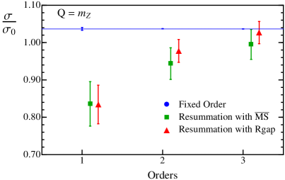
Figure -1259: Theoretical computations at various orders in perturbation theory for the total hadronic cross section at the Z-pole normalized to the Born-level cross section $\sigma_{0}$. Here the small blue points correspond to fixed order perturbation theory, green squares to resummation without renormalon subtractions, and red triangles to resummation with renormalon subtractions.

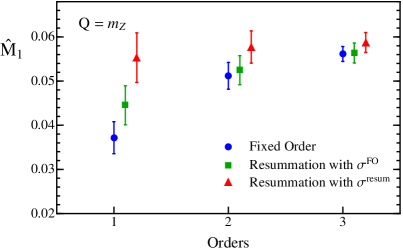
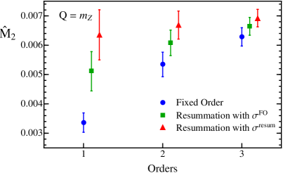
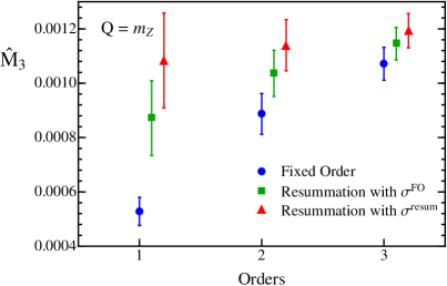
Figure -1258: Theoretical prediction for the first three moments at the Z-pole at various orders in perturbation theory. The blue circles correspond to fixed order perturbation theory (normalized with the total hadronic cross section) at ${\cal O}(\alpha_{s})$, ${\cal O}(\alpha_{s}^{2})$ and ${\cal O}(\alpha_{s}^{3})$, green squares correspond to resummed predictions at NLL, NNLL, and N³LL normalized with the total hadronic cross section, and red triangles correspond to resummation normalized with the norm of the resummed distribution. For these plots we use $\alpha_{s}(m_{Z})=0.114$.

For our moment analysis we use the thrust distribution code developed in Ref. Abbate et al. (2011), where a detailed description of the various ingredients may be found. We are able to perform fits with different level of accuracy: fixed order at $\mathcal{O}(\alpha_{s}^{3})$, resummation of large logarithms to N³LL accuracy, power corrections, and subtraction of the leading renormalon ambiguity. Recently the complete calculation of the ${\cal O}(\alpha_{s}^{2})$ hemisphere soft function has become available Kelley et al. (2011); Hornig et al. (2011); Monni et al. (2011), so the code is updated to use the fixed parameter $s_{2}=-40.6804$ from Refs. Kelley et al. (2011); Monni et al. (2011). A feature of our code is its ability to describe the thrust distribution in the whole range of thrust values. This is achieved with the introduction of what we call profile functions, which are $\tau$-dependent factorization scales. In the $e^{+}\,e^{-}$ annihilation process there are three relevant scales: hard, jet and soft, associated to the center of mass energy, the jet mass and the energy of soft radiation, respectively. The purpose of $\tau$-dependent profile functions for these scales is to smoothly interpolate between the peak region where we must ensure that $\mu_{i}>\Lambda_{\rm QCD}$, the dijet region where the summation of large logs is crucial, and the multijet region where regular perturbation theory is appropriate to describe the partonic contribution Abbate et al. (2011). The major part of the higher order perturbative uncertainties are directly related to the arbitrariness of the profile functions, and are estimated by scanning the space of parameters that specify them. For details on the profile functions and the parameter scans we refer the reader to App. A. We note that our distribution code was designed for $Q$ values above $22$ GeV.

III.1 Ingredients

The theoretical fixed order expression for the thrust moments contain no large logarithms, so we might not expect that the resummation of logarithms in the thrust spectrum will play a role in the numerical analysis. We will show that there is nevertheless some benefit in accounting for the resummation of thrust logarithms. This is studied in Figs. -1259 and -1258, where for $Q=m_{Z}$ we compare the theoretical value of moments of the thrust distribution obtained in fixed order with those obtained including resummation. (The error bars for the fixed order expansion arise from varying the renormalization scale $\mu$ between $Q/2$ and $2\,Q$ and those for the resummed results arise from our theory parameter scan method.)

In Fig. -1259 we show the total hadronic cross section $\sigma$ from the fixed order $\alpha_{s}$ expansion (blue points with small uncertainties sitting on the horizontal line) and determined from the integral over the log-resummed distribution with/without renormalon subtractions (red triangles and green squares). Both expansions are displayed including fixed order corrections up to order $\alpha_{s}(m_{Z})$, $\alpha_{s}^{2}(m_{Z})$ and $\alpha_{s}^{3}(m_{Z})$, as indicated by the orders 1, 2, 3, respectively. We immediately notice that the resummed result is not as effective in reproducing the total cross section as the fixed order expansion. Predictions that sum large logarithms have a substantial (perturbative) normalization uncertainty. On the other hand, as shown in Ref. Abbate et al. (2011), the resummation of logarithms combined with the profile function approach leads to a description of the thrust spectrum that converges nicely over the whole physical $\tau$ range when the norm of the spectrum is divided out, a property not present in the spectrum of the fixed order expansion.

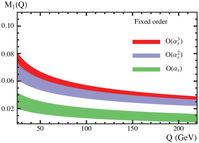
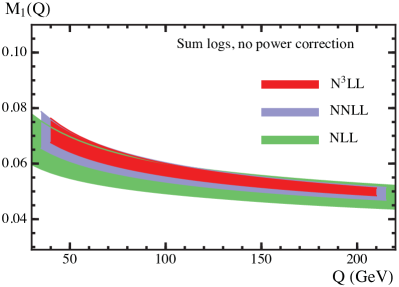
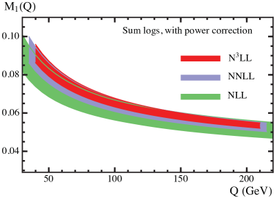
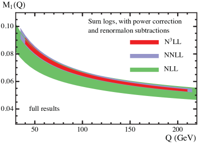
Figure -1257: Theory scan for uncertainties in pure QCD with massless quarks. The panels are fixed order (top-left), resummation without the nonperturbative correction (top-right), resummation with a nonperturbative function using the $\overline{\textrm{MS}}$ scheme for $\overline{\Omega}_{1}$ (bottom-left), resummation with renormalon subtraction and a nonperturbative function in the Rgap scheme for $\Omega_{1}$ (bottom-right).

In Fig. -1258 the expansions of the partonic moments $\hat{M}_{1}$, $\hat{M}_{2}$, and $\hat{M}_{3}$ are displayed in the fixed order expansion (blue circles) and the log-resummed result with either the fixed order normalization (green squares) or a properly normalized spectrum (red triangles). We observe that the fixed order expansion has rather small variations from scale variation, but shows poor convergence indicating that its renormalization scale variation underestimates the perturbative uncertainty. For $\hat{M}_{1}$ the fixed order and log-resummed expressions with a common fixed-order normalization (blue circles and green squares) agree well at each order, indicating that, as expected, large logarithms do not play a significant role for this moment. On the other hand, the expansion based on the properly normalized log-resummed spectrum exhibits excellent convergence, and also has larger perturbative uncertainties at the lowest order. In particular, for the red triangles the higher order results are always within the 1-$\sigma$ uncertainties of the previous order. The result shows that using the normalized log-resummed spectrum for thrust, which converges nicely for all $\tau$, also leads to better convergence properties of the moments. At third order all the fixed order and resummed partonic moments are consistent with each other. Since the log-resummed moments exhibit more realistic estimates of perturbative uncertainties at each order, we will use the normalized resummed moments for our fit analysis.

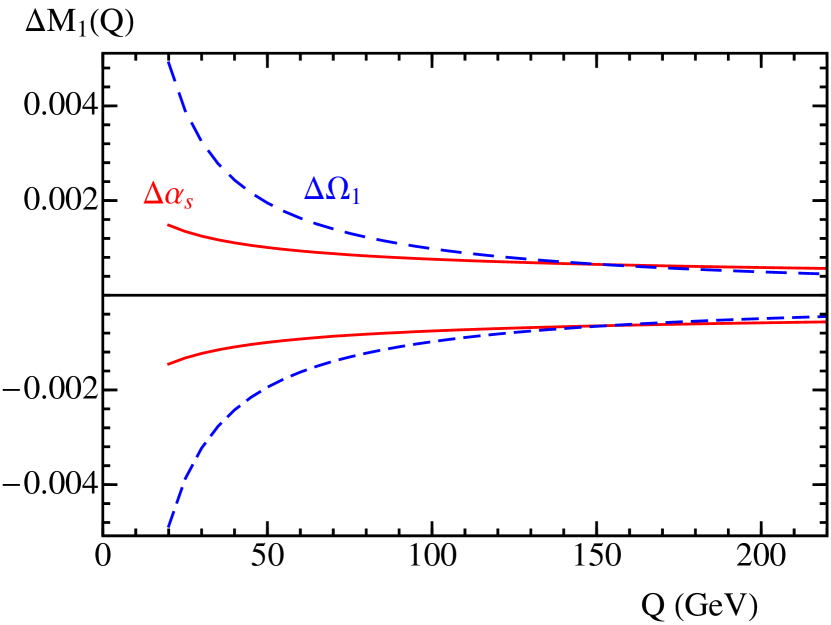
Figure -1256: Difference between theoretical predictions with default parameters for the first moment as function of $Q$ when varying one parameter at a time. The red solid line corresponds to varying $\Delta\alpha_{s}(m_{Z})=\pm 0.001$ and the blue dashed lines to varying $\Delta\Omega_{1}=\pm 0.1$, with respect to the pure QCD best-fit values. There is a strong degeneracy of the two parameters in the region $Q>100$ GeV, which is obviously broken when considering values of $Q$ below $70$ GeV.

In Fig. -1257 we show how the inclusion of various ingredients (fixed order contributions, log resummation, power corrections, renormalon subtraction) affects the convergence and uncertainty of our theoretical prediction for the first moment of the thrust distribution as a function of $Q$. From these plots we can observe four points: i) Fixed order perturbation theory does not converge very well. ii) Resummation of large logarithms in the distribution, when normalized with the integral of the resummed distribution, improves convergence for every center of mass energy. iii) The inclusion of power corrections has the effect of a $1/Q$-modulated vertical shift on the value of the first moment. iv) The subtraction of the renormalon ambiguity reduces the theoretical uncertainty. This picture for the first moment is consistent with the results of Ref. Abbate et al. (2011) for the thrust distribution.

Another important element of our analysis is that we perform global fits, simultaneously using data at a wide range of center of mass energies $Q$. This is motivated by the fact that for each $Q$ there is a complete degeneracy between changing $\alpha_{s}(m_{Z})$ and changing $\Omega_{1}$, which can be lifted only through a global analysis. Fig. -1256 shows the difference between the theoretical prediction of $M_{1}$ as a function of $Q$, when $\alpha_{s}(m_{Z})$ or $\Omega_{1}$ are varied by $\pm\,0.001$ and $\pm\,0.1$ GeV, respectively. We see that the effect of a variation in $\alpha_{s}(m_{Z})$ can be compensated with an appropriate variation in $\Omega_{1}$ at a given center of mass energy (or in a small $Q$ range). This degeneracy is broken if we perform a global fit including the wide range of $Q$ values shown in the figure.

Finally, in Fig. -1255 we show $\alpha_{s}(m_{Z})$ extracted from fits to the first moment of the thrust distribution at three-loop accuracy including sequentially the different effects our code has implemented: O$(\alpha_{s}^{3})$ fixed order, N³LL resummation, power corrections, renormalon subtraction, b-quark mass and QED. The error bars of the first two points at the left hand side do not contain an estimate of uncertainties associated with the power correction. Though smaller, the resummed result is compatible at the 1-$\sigma$ level with the fixed order result. The inclusion of the power correction is the element which has the greatest impact on $\alpha_{s}(m_{Z})$; for the $\overline{\textrm{MS}}$ definition of $\Omega_{1}$ it reduces the central value by 7%. The subtraction of the renormalon ambiguity in the Rgap scheme reduces the theoretical uncertainty by a factor of 3, while b-quark mass and QED effects give negligible contributions with current uncertainties.

order	$\alpha_{s}(m_{Z})$ (with $\overline{\Omega}_{1}^{\overline{\textrm{MS}}}$)	$\alpha_{s}(m_{Z})$ (with $\Omega_{1}^{\rm Rgap}$)
NLL	$0.1173(82)(13)$	$0.1172(82)(13)$
NNLL	$0.1159(41)(14)$	$0.1139(15)(13)$
N3LL (full)	$0.1153(21)(14)$	$\mathbf{0.1140(07)(14)}$
N3LL (QCD+$m_{b}$)	$0.1160(20)(14)$	$0.1146(07)(14)$
N3LL (pure QCD)	$0.1156(21)(14)$	$0.1142(07)(14)$

Table 1: Central values for $\alpha_{s}(m_{Z})$ at various orders with theory uncertainties from the parameter scan (first value in parentheses), and experimental and hadronic error added in quadrature (second value in parentheses). The bold N³LL value above the line is our final result, while values below the line show the effect of leaving out the QED and $b$-mass corrections.

order	$\overline{\Omega}_{1}$ ($\overline{\textrm{MS}}$) [GeV]	$\Omega_{1}$ (Rgap) [GeV]
NLL	$0.504(157)(45)$	$0.500(153)(45)$
NNLL	$0.405(82)(47)$	$0.413(43)(44)$
N3LL (full)	$0.318(75)(49)$	$\mathbf{0.377(39)(44)}$
N3LL (QCD+$m_{b}$)	$0.310(74)(49)$	$0.369(34)(44)$
N3LL (pure QCD)	$0.350(67)(49)$	$0.402(35)(44)$

Table 2: Central values for $\Omega_{1}$ at the reference scales $R_{\Delta}=\mu_{\Delta}=2$ GeV and for $\overline{\Omega}_{1}$ and at various orders. The parentheses show theory uncertainties from the parameter scan, and experimental and hadronic uncertainty added in quadrature, respectively. The bold value above the line is our final result, while the N³LL values below the horizontal line show the effect of leaving out the QED and $b$-mass corrections.

	$\alpha_{s}(m_{Z})$	$\chi^{2}/({\rm dof})$
N3LL with $\Omega_{1}^{\rm Rgap}$	$0.1140(07)(14)$	$1.33$
N3LL with $\overline{\Omega}_{1}^{\overline{\textrm{MS}}}$	$0.1153(21)(14)$	$1.33$
N3LL no power corr.	$0.1236(39)(03)$	$2.03$
${\cal O}(\alpha_{s}^{3})$ fixed order no power corr.	$0.1305(39)(04)$	$2.52$

Table 3: Comparison of first moment fit results for analyses with full results and $\Omega_{1}=\Omega_{1}^{\rm Rgap}$, with $\overline{\Omega}_{1}$ and no renormalon subtractions, without power corrections, and at fixed order without power corrections or log resummation. The first number in parentheses corresponds to the theory uncertainty, whereas the second corresponds to the experimental and hadronic uncertainty added in quadrature for the first two rows, and experimental uncertainty for the last two rows.

III.2 Uncertainty Analysis

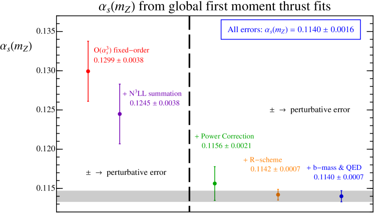
Figure -1255: Evolution of the best-fit values for $\alpha_{s}(m_{Z})$ from thrust first moment fits when including various levels of improvement with respect to fixed order QCD. Only points at the right of the vertical dashed line include nonperturbative effects.

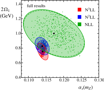
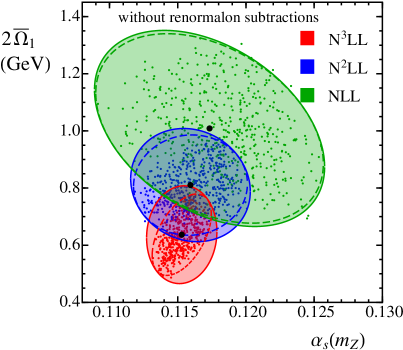
Figure -1254: Distribution of best-fit points in the $\alpha_{s}(m_{Z})$-$2\,\Omega_{1}$ and $\alpha_{s}(m_{Z})$-$2\,\overline{\Omega}_{1}$ planes. The left panel shows results including perturbation theory, resummation of the logs, the soft nonperturbative function, and $\Omega_{1}$ defined in the Rgap scheme with renormalon subtractions. The right panel shows the same results, but with $\overline{\Omega}_{1}$ defined in the $\overline{\textrm{MS}}$ scheme, and without renormalon subtractions. In both panels the dashed lines corresponds to an ellipse fit to the contour of the best-fit points to determine the theoretical uncertainty. The respective total (experimental + theoretical) 39% CL standard error ellipses are displayed (solid lines), which correspond to $1$-$\sigma$ (68% CL) for either one-dimensional projection.

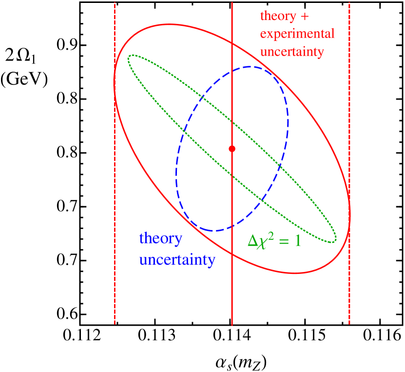
Figure -1253: Experimental $\Delta\chi^{2}=1$ standard error ellipse (dotted green) at N³LL accuracy with renormalon subtractions, in the $\alpha_{s}$-$2\,\Omega_{1}$ plane. The dashed blue ellipse represents the theory uncertainty which is obtained by fitting an ellipse to the contour of the distribution of the best-fit points. This ellipse should be interpreted as the $1$-$\sigma$ theory uncertainty for $1$-parameter (39% confidence for $2$-parameters). The solid red ellipse represents the total (combined experimental and perturbative) uncertainty ellipse.

In Fig. -1254 we show the result of our theory scan to determine the perturbative uncertainties. At each order we carried out 500 fits, with theory parameters randomly chosen in the ranges given in Table 8 of App. A (where further details may be found). The left panel of Fig. -1254 shows results with renormalon subtractions using the Rgap scheme for $\Omega_{1}$, and the right-panel shows results in the $\overline{\textrm{MS}}$ scheme without renormalon subtractions. Each point in the plot represents the result of a single fit. As described in App. A, in order to estimate perturbative uncertainties, we fit an ellipse to the contour of best-fit points in the $\alpha_{s}$-$2\,\Omega_{1}$ plane, and we interpret this as 1-$\sigma$ theoretical error ellipse. This is represented by the dashed lines in Fig. -1254. The solid lines represent the combined (theoretical and experimental) standard error ellipses. These are obtained by adding the theoretical and experimental error matrices which determined the individual ellipses. The central values of the fits, collected in Tables 1 and 2, are determined from the average of the maximal and minimal values of the theory scan, and are very close to the central values obtained when running with our default parameters. The minimal $\chi^{2}$ values for these fits are quoted in Table 3 as well. The best fit based on our full code has $\chi^{2}/{\rm dof}=1.325\pm\,0.002$ where the range incorporates the variation from the displayed scan points at N³LL. The fit results show a substantial reduction of the theoretical uncertainties with increasing perturbative order. Removal of the $\mathcal{O}(\Lambda_{\rm QCD})$ renormalon improves the perturbative convergence and leads to a reduction of the theoretical uncertainties at the highest order by a factor of 2 in $\Omega_{1}$, and factor of 3 in $\alpha_{s}(m_{Z})$

To analyze in detail the experimental and the total uncertainties of our results, we refer now to Fig. -1253. Here we show the error ellipses for our highest order fit, which includes resummation, power corrections, renormalon subtraction, QED and b-quark mass contributions. The green dotted, blue dashed, and the solid red lines represent the standard error ellipses for, respectively, experimental, theoretical, and combined theoretical and experimental uncertainties. The experimental and theory error ellipses are defined by $\Delta\chi^{2}=1$ since we are most interested in the 1-dimensional projection onto $\alpha_{s}$. The correlation matrix of the experimental, theory, and total error ellipses are ($i,j=\alpha_{s},2\,\Omega_{1}$)

$$V_{ij} =\,\left(\begin{array}[]{cc}\sigma_{\alpha_{s}}^{2}&\,\,2\sigma_{\alpha_{s}}\sigma_{\Omega_{1}}\rho_{\alpha\Omega}\\ 2\sigma_{\alpha_{s}}\sigma_{\Omega_{1}}\rho_{\alpha\Omega}&\,\,4\sigma_{\Omega_{1}}^{2}\end{array}\right),$$ (31)

$$V^{\rm exp}_{ij} =\left(\begin{array}[]{cc}1.93(15)\cdot 10^{-6}&\,\,-1.18(13)\cdot 10^{-4}\,\mbox{GeV}\\ -1.18(13)\cdot 10^{-4}\,\mbox{GeV}&\,\,0.79(13)\cdot 10^{-2}\,\mbox{GeV}^{2}\end{array}\right)\!,$$ (34)

$$V^{\rm theo}_{ij} =\left(\begin{array}[]{cc}5.56\cdot 10^{-7}&\,\,1.85\cdot 10^{-5}~{}\mbox{GeV}\\ 1.85\cdot 10^{-5}~{}\mbox{GeV}&\,\,5.82\cdot 10^{-3}~{}\mbox{GeV}^{2}\end{array}\right),$$ (37)

$$V^{\rm tot}_{ij} =\left(\begin{array}[]{cc}2.49(15)\cdot 10^{-6}&\,\,-0.99(13)\cdot 10^{-4}\,\mbox{GeV}\\ -0.99(13)\cdot 10^{-4}\,\mbox{GeV}&\,\,1.37(13)\cdot 10^{-2}\,\mbox{GeV}^{2}\end{array}\right)\!,$$ (40)

where the experimental correlation coefficient is significant and reads

$$\rho^{\rm exp}_{\alpha\Omega}\,=\,-\,0.96(14)\,.$$ (41)

Adding the theory scan uncertainties reduces the correlation coefficient in Eq. (41) to

$$\rho_{\alpha\Omega}^{\rm total}\,=\,-\,0.54(8).$$ (42)

In both Eqs. (41) and (42) the numbers in parentheses capture the range of values obtained from the theory scan. From $V_{ij}^{\rm exp}$ in Eq. (31) it is possible to extract the experimental uncertainty for $\alpha_{s}$ and $\Omega_{1}$ and the uncertainty due to variations of $\Omega_{1}$ and $\alpha_{s}$, respectively:

$$\sigma_{\alpha_{s}}^{\rm exp} =\,\sigma_{\alpha_{s}}\,\sqrt{1-\rho^{2}_{\alpha\Omega}}=\,0.0004\,,$$ (43)

$$\sigma_{\Omega_{1}}^{\rm exp} =\,\sigma_{\Omega_{1}}\,\sqrt{1-\rho^{2}_{\alpha\Omega}}=\,0.013~{}\mbox{GeV}\,,$$

$$\sigma_{\alpha_{s}}^{\rm\Omega_{1}} =\,\sigma_{\alpha_{s}}\,|\rho_{\alpha\Omega}|\,=\,0.0014\,,$$

$$\sigma_{\Omega_{1}}^{\rm\alpha_{s}} =\,\sigma_{\Omega_{1}}\,|\rho_{\alpha\Omega}|\,=\,0.044~{}\mbox{GeV}\,.$$

Fig. -1253 shows the total uncertainty in our final result quoted in Eq. (45) below.

The correlation exhibited by the green dotted experimental error ellipse in Fig. -1253 is given by the line describing the semimajor axis

$$\frac{\Omega_{1}}{32.82\,{\rm GeV}}=0.1255-\alpha_{s}(m_{Z})\,.$$ (44)

Note that extrapolating this correlation to the extreme case where we neglect the nonperturbative corrections ($\Omega_{1}=0$) gives $\alpha_{s}(m_{Z})\to 0.1255$.

III.3 Effects of QED and the $b$-mass

The experimental correction procedures applied to the AMY, JADE, SLC, DELPHI and OPAL data sets were typically designed to eliminate initial state photon radiation, while those of the TASSO, L3 and ALEPH collaborations eliminated initial and final state photon radiation. It is straightforward to test for the effect of these differences in the fits by using our theory code with QED effects turned on or off depending on the data set. Using our N³LL order code in the Rgap scheme we obtain the central values $\alpha_{s}(m_{Z})=0.1143$ and $\Omega_{1}=0.376$ GeV. Comparing to our default results given in Tabs. 1 and 2, which are based on the theory code were QED effects are included for all data sets, we see that the central value for $\alpha_{s}$ is larger by $0.0003$ and the one for $\Omega_{1}$ is smaller by $0.001$ GeV. This shift is substantially smaller than our perturbative uncertainty. Hence our choice to use the theory code with QED effects included everywhere as the default for our analysis does not cause an observable bias regarding experiments which remove final state photons.

By comparing the N³LL (pure massless QCD) and N³LL (QCD $+\,m_{b}$) entries in Tabs. 1 and 2 we see that including finite $b$-mass corrections causes a very mild shift of $\simeq+0.0004$ to $\alpha_{s}(m_{Z})$, and a somewhat larger shift of $\simeq-0.033\,{\rm GeV}$ to $\Omega_{1}$. In both cases these shifts are within the 1-$\sigma$ theory uncertainties. In the N³LL (pure massless QCD) analysis the $b$-quark is treated as a massless flavor, hence this analysis differs from that done by JADE Pahl et al. (2009a) where primary $b$ quarks were removed using MC generators.

III.4 Final Results

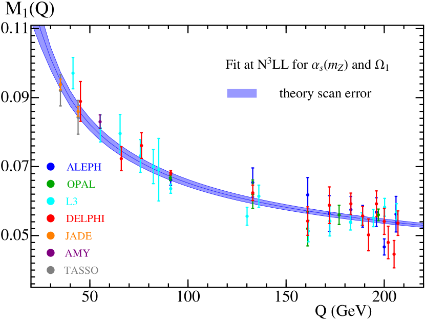
Figure -1252: First moment of the thrust distribution as a function of the center of mass energy $Q$, using the best-fit values for $\alpha_{s}(m_{Z})$ and $\Omega_{1}$ in the Rgap scheme as given in Eq. (45). The blue band represents the perturbative uncertainty determined by our theory scan. Data is from ALEPH, OPAL, L3, DELPHI, JADE, AMY and TASSO.

As our final result for $\alpha_{s}(m_{Z})$ and $\Omega_{1}$, obtained at N³LL order in the Rgap scheme for $\Omega_{1}(R_{\Delta},\mu_{\Delta})$, including bottom quark mass and QED corrections we obtain

$$\alpha_{s}(m_{Z}) \,=\,0.1140\,\pm\,(0.0004)_{\rm exp}$$ (45)

$$\,\pm\,(0.0013)_{\rm hadr}\,\pm\,(0.0007)_{\rm pert},$$

$$\Omega_{1}(R_{\Delta},\mu_{\Delta}) \,=\,0.377\,\pm\,(0.013)_{\rm exp}$$

$$\,\pm\,(0.042)_{\rm\alpha_{s}(m_{Z})}\,\pm\,(0.039)_{\rm pert}~{}\mbox{GeV},$$

where $R_{\Delta}=\mu_{\Delta}=2$ GeV and we quote individual $1$-$\sigma$ uncertainties for each parameter. Here $\chi^{2}/\rm{dof}=1.33$. Eq. (45) is the main result of this work.

In Fig. -1252 we show the first moment of the thrust distribution as a function of the center of mass energy $Q$, including QED and $m_{b}$ corrections. We use here the best-fit values given in Eq. (45). The band displays the theoretical uncertainty and has been determined with a scan on the parameters included in our theory, as explained in App. A. The fit result is shown in comparison with data from ALEPH, OPAL, L3, DELPHI, JADE, AMY and TASSO. Good agreement is observed for all $Q$ values.

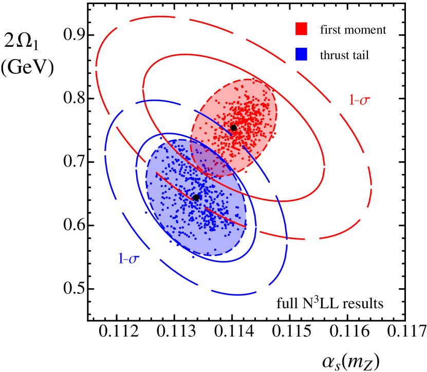
Figure -1251: Comparison of $\alpha_{s}(m_{Z})$ and $\Omega_{1}$ determinations from thrust first moment data (red upper right ellipses) and thrust tail data (blue lower left ellipses). The plot corresponds to fits with N³LL accuracy and in the Rgap scheme. The tail fits are performed with our improved code which uses a new nonsingular two-loop function, and the now known two-loop soft function. Dashed lines correspond to theory uncertainties, solid lines correspond to $\Delta\chi^{2}=1$ combined theoretical and experimental error ellipses, and wide-dashed lines correspond to $\Delta\chi^{2}=2.3$ combined error ellipses (corresponding to 1-$\sigma$ uncertainty in two dimensions).

It is interesting to compare the result of this analysis with the result of our earlier fit of thrust tail distributions in Ref. Abbate et al. (2011). This is shown in Fig. -1251. Here the red upper shaded area and corresponding ellipses show the results from fits to the first moment of the thrust distribution, while the blue lower shaded area and ellipses show the result from fits of its tail region. Both analyses show the theory (dashed lines) and combined theoretical and experimental (solid lines) standard error ellipses, as well as the ellipses which correspond to $\Delta\chi^{2}=2.3$ (68% CL for a two-parameter fit, wide-dashed lines). We see that the two analyses are compatible.

IV Fixed Order Analysis of $M_{1}$

It is interesting to compare the result of our best fit with an analysis where we do not perform resummation in the thrust distribution, but where power corrections and renormalon subtractions are still considered. This is achieved by setting the scales $\mu_{H}$, $\mu_{S}$, $\mu_{J}$, $\mu_{\rm ns}$ in our theoretical prediction all to a common scale $\mu\sim Q$. We use $R$ for the scale of the renormalon subtractions and renormalization group evolved power correction. Finally we will neglect QED and $b$-mass corrections in this subsection. Up to the treatment of power corrections and perturbative subtractions, the fixed order results used for this analysis are thus equivalent to those used in Ref. Gehrmann et al. (2010).

The OPE formula for the first moment in the Rgap scheme for this situation is given by

$$M_{1} ={\hat{M}}_{1}^{\rm Rgap}(R,\mu)+\dfrac{2\,\Omega_{1}(R,\mu)}{Q}\,,$$ (46)

$$\Omega_{1}(R,\mu) =\Omega_{1}+\bar{\Delta}(R,\mu)-\bar{\Delta}(R_{\Delta},\mu_{\Delta})\,,$$

In Eq. (46), the $\Omega_{1}$ with no arguments is the value determined by the fits, which is in the Rgap scheme at the reference scale $\mu_{\Delta}=R_{\Delta}=2\,{\rm GeV}$. Here $\bar{\Delta}(R,\mu)$ is the running gap parameter, and $\bar{\Delta}(R,\mu)-\bar{\Delta}(R_{\Delta},\mu_{\Delta})$ is used to sum logarithms from $(R_{\Delta},\mu_{\Delta})$ to $(R,\mu)$ in Eq. (46). The analytic expression for $\bar{\Delta}(R,\mu)-\bar{\Delta}(R_{\Delta},\mu_{\Delta})$ can be found in Eq. (41) of Ref. Abbate et al. (2011) (see also Hoang and Kluth (2008)). The perturbative ${\hat{M}}_{1}^{\rm Rgap}$ is related to the perturbative $\overline{\textrm{MS}}$ result by

$${\hat{M}}_{1}^{\rm Rgap}(R,\mu) ={\hat{M}}_{1}^{\rm\overline{MS}}(\mu)+\dfrac{2\,\delta(R,\mu)}{Q}\,,$$ (47)

$$\delta(R,\mu) =e^{\gamma_{E}}R\sum_{i=1}^{3}\alpha_{s}(\mu)^{i}\delta_{i}(R,\mu)\,,$$

where the subtractions terms are Hoang and Kluth (2008); Abbate et al. (2011)

$$\delta_{1}(R,\mu) =-0.848826L_{R}\,,$$ (48)

$$\delta_{2}(R,\mu) =-0.156279-0.46663L_{R}-0.517864L_{R}^{2}\,,$$

$$\delta_{3}(R,\mu) =-\,0.552986-0.622467L_{R}-0.777219L_{R}^{2}$$

$$\quad-0.421261L_{R}^{3}\,,$$

with $L_{R}=\ln(\mu/R)$. In Eq. (47) $\delta(R,\mu)$ cancels the ${\cal O}(\Lambda_{\rm QCD})$ renormalon in ${\hat{M}}_{1}^{\rm\overline{MS}}(\mu)$, and it is crucial that the coupling expansions in both these objects are done at the same scale, $\alpha_{s}(\mu)$, for this cancellation to take place. The relation to the $\overline{\textrm{MS}}$ scheme power correction is $\overline{\Omega}_{1}=\Omega_{1}+\delta(R_{\Delta},\mu_{\Delta})$, and the OPE in the $\overline{\textrm{MS}}$ scheme at this level is

$$M_{1} ={\hat{M}}_{1}^{\overline{\rm MS}}(\mu)+\dfrac{2\,{\overline{\Omega}}_{1}}{Q}\,.$$ (49)

In the $\overline{\textrm{MS}}$ result there are no perturbative renormalon subtractions (and thus no log resummation related to the renormalon subtractions) and the parameter $\overline{\Omega}_{1}$ has a $\Lambda_{\rm QCD}$ renormalon ambiguity.

We will perform fits to the experimental data following the same procedure discussed in the previous section. Using Eq. (46) we consider two cases, i) $R\sim Q$ where $\Omega_{1}$ is renormalization group evolved to $R$ and there are no large logarithms in the renormalon subtractions, and ii) fixing $R$ at the reference scale, $R=2\,{\rm GeV}$, in which case large logarithms are present in the renormalon subtractions. We will also consider a third case, iii), using the $\overline{\textrm{MS}}$-OPE of Eq. (49).

order	${\cal O}(\alpha_{s}^{2})$	${\cal O}(\alpha_{s}^{3})$
(i) Rgap R-RGE	$0.1159(27)(14)$	$0.1146(06)(14)$
(ii) Rgap FO Subt.	$0.1185(63)(15)$	$0.1138(20)(14)$
(iii) $\overline{\textrm{MS}}$ for ${\overline{\Omega}}_{1}$	$0.1278(124)(19)$	$0.1186(38)(14)$

Table 4: $\overline{\textrm{MS}}$ scheme values for $\alpha_{s}(m_{Z})$ obtained from various fixed order analyses. The first value in parentheses is the uncertainty from higher order perturbative corrections (obtained by the method described in the text), while the second value is the combined experimental and hadronization uncertainty.

order	${\cal O}(\alpha_{s}^{2})$	${\cal O}(\alpha_{s}^{3})$
(i) Rgap R-RGE	$0.407(8)(45)$	$0.400(8)(45)$
(ii) Rgap FO Subt.	$0.216(126)(133)$	$0.359(42)(62)$
(iii) $\overline{\textrm{MS}}$ for ${\overline{\Omega}}_{1}$	$0.388(62)(47)$	$0.350(54)(44)$

Table 5: $\Omega_{1}$ or $\overline{\Omega}_{1}$ values obtained from fixed order analyses at various orders. The first value in parentheses is the uncertainty from higher order perturbative corrections (obtained by the method described in the text), while the second value is the combined experimental and hadronization uncertainty.

Results for these fits are shown in Tabs. 4 and 5. For all cases $\chi^{2}/\rm{dof}\simeq 1.32$.

For case i) we take $R\sim\mu\sim Q$, so there are no large logarithms in the $\delta(R,\mu)$ of Eq. (46), and all large logarithms associated with renormalon subtractions are summed in $\bar{\Delta}(R,\mu)-\bar{\Delta}(R_{\Delta},\mu_{\Delta})$. Here we estimate the perturbative uncertainty in $\alpha_{s}(m_{Z})$ and $\Omega_{1}$ by varying the renormalization scale $\mu$ and the scale $R$ independently in the range $\{2\,Q,Q/2\}$. We use one-half the maximum minus minimum variation as the uncertainty, and the average for the central value. The results for both $\alpha_{s}(m_{Z})$ and $\Omega_{1}$ are fully compatible at 1-$\sigma$ to our final results shown in Eq. (45). The agreement is even closer to the central values for the fits without QED or $b$-mass corrections in Tabs. 1 and 2, namely $\alpha_{s}(m_{Z})=0.1142(07)(14)$ and $\Omega_{1}=0.402(35)(44)$. The one difference is that the perturbative uncertainty for $\Omega_{1}$ in Tab. 5 is a factor of three smaller. The case i) results in the table also exhibit nice order-by-order convergence, and if one plots $M_{1}$ versus $Q$ (analogous to Fig. -1258) the uncertainty bands are entirely contained within one another. In order to be conservative, we take our resummation analysis in Eq. (45) as our final results (with its larger perturbative uncertainty and inclusion of QED and $b$-mass corrections).

For case ii) we take $R\sim 2\,{\rm GeV}$ and $\mu\sim Q$ as typical values, so there are large logarithms, $\ln(R/Q)$, in the $\delta(R,\mu)$ renormalon subtractions. The central value for $\alpha_{s}(m_{Z})$ at ${\cal O}(\alpha_{s}^{3})$ is again fully compatible with that in Eq. (45). Here we estimate the perturbative uncertainty in $\alpha_{s}(m_{Z})$ by varying $\mu\in\{2\,Q,Q/2\}$ and $R=2\pm 1\,{\rm GeV}$. Due to the large logarithms the perturbative uncertainty in $\alpha_{s}(m_{Z})$ for case ii), shown in Tab. 4, is three times larger than for case i). It is also compatible with the difference between central values at ${\cal O}(\alpha_{s}^{2})$ and ${\cal O}(\alpha_{s}^{3})$. To estimate the uncertainty for $\Omega_{1}$ we only vary $\mu$, which leads to the rather large error estimate for $\Omega_{1}$ shown in Tab. 5. The contrast between the precision of the results in case i), to the results in case ii), illustrates the importance of summing large logarithms in the renormalon subtractions.

For case iii), where the ${\overline{\Omega}}_{1}$ power correction is defined in $\overline{\textrm{MS}}$ we do not have renormalon subtractions (and hence no large logs in subtractions). Due to the poor convergence of the fixed order prediction for the first moment, seen from the blue fixed order points in Fig. -1258, it is not clear whether varying $\mu$ in the range $\{2\,Q,Q/2\}$ gives a realistic perturbative uncertainty estimate. Hence we determine the perturbative uncertainty for case iii) in Tabs. 4 and 5 by varying $\mu$ in the range $\{2\,Q,Q/2\}$ and multiply the result by a factor of two. The perturbative uncertainties for $\alpha_{s}(m_{Z})$ are a factor of two larger than in case ii). The central values for $\alpha_{s}(m_{Z})$ in case iii) are also larger, but are compatible with those in case ii) and Eq. (45) within 1-$\sigma$.

It is interesting to compare our results to those of Ref. Gehrmann et al. (2010), which also performs a fixed order analysis at ${\cal O}(\alpha_{s}^{3})$, and incorporates subtractions based on the dispersive model. Here the subtractions contain logarithms, $\ln(\mu_{I}/\mu)$, where $\mu_{I}\sim 2\,{\rm GeV}$ and $\mu\sim Q$, that are not resummed. From a fit to $M_{1}$ in thrust they obtained $\alpha_{s}(m_{Z})\,=\,0.1166\,\pm\,0.0015_{\rm exp}\,\pm\,0.0032_{\rm th}$ where the first uncertainty is experimental and the second is theoretical. Our corresponding result is the one in case ii), and the central values and uncertainties for $\alpha_{s}(m_{Z})$ are fully compatible. The perturbative uncertainty they obtain is a factor of $1.6$ larger than ours. It arises from varying the renormalization scale $\mu\in\{2\,Q,Q/2\}$, the ${\cal O}(\alpha_{s}^{2})$ Milan factor $\cal M$ by 20%, and the infrared scale $\mu_{I}=2\pm 1\,{\rm GeV}$ in the dispersive model. In our analysis there is no precise analog of the Milan factor because our subtractions and Rgap scheme for $\Omega_{1}$ fully account for two and three gluon infrared effects up to ${\cal O}(\alpha_{s}^{3})$ that are associated to thrust. Other than this, the difference can be simply attributed to the differences in subtraction schemes which have an impact on the $\mu$ scale uncertainty. Finally, note that we have implemented the analytic results of Ref. Gehrmann et al. (2010) and confirmed their $\mu$ and $\mu_{I}$ uncertainties.

V JADE Datasets

As discussed in Sec. I our global dataset includes thrust moment results from ALEPH, OPAL, L3, DELPHI, AMY, TASSO and the JADE data from Ref. Movilla Fernandez et al. (1998). In this section we discuss the impact on the results in Secs. III and IV of replacing the JADE data from Ref. Movilla Fernandez et al. (1998) with moment results from an updated analysis carried out in Ref. Pahl et al. (2009a), which removes the contributions from primary $b\bar{b}$ pair production and provides in addition measurements at $Q=14$ and $22$ GeV. In Fig. -1250 we show the data for $M_{1}$, including the JADE results from Refs. Movilla Fernandez et al. (1998) and Pahl et al. (2009a). The most significant difference occurs at $Q=44\,{\rm GeV}$. Our analysis will treat these datasets on the same footing without attempting to account for the effect of removing the $b\bar{b}$’s.

For our analysis here, with theory results at N³LL + ${\cal O}(\alpha_{s}^{3})$, we continue to exclude center of mass energies $Q\leq 22$ GeV as in Sec. III. The dependence of the global fit result on the data set for $M_{1}$ is shown in Fig. -1249. Theoretical uncertainties are analyzed again by the scan method giving the central dots and three inner ellipses, while the outer three ellipses show the respective combined 1-$\sigma$ total experimental and theoretical uncertainties. Using all experimental data but excluding JADE measurements entirely gives the fit result shown by the upper blue ellipse. This result is compatible at 1-$\sigma$ with the central red ellipse which shows our default analysis, using the Ref. Movilla Fernandez et al. (1998) JADE $M_{1}$ measurements. Replacing these two JADE data points by the four $Q>22\,{\rm GeV}$ JADE $M_{1}$ results from Ref. Pahl et al. (2009a) yields the lower green ellipse (whose center is $\simeq 1.5$-$\sigma$ from the central ellipse). For this fit the $\chi^{2}/{\rm dof}$ increases from $1.33$ to $1.52$ demonstrating that there is less compatibility between the data. For this reason, together with the concern about the impact of removing primary $b\bar{b}$ events with MC simulations, we have used only JADE data from Ref. Movilla Fernandez et al. (1998) in our main analysis.

A similar pattern is observed using the fixed order fits of $M_{1}$ discussed in Sec. IV. In this case it is also straightforward to include the $Q=14,22\,{\rm GeV}$ JADE data from Ref. Pahl et al. (2009a). If these two points are added to our default dataset (which contains $Q=35$ and $45$ GeV as the lowest $Q$ results for $M_{1}$) then we find $\alpha_{s}(m_{Z})=0.1155\pm 0.0012$ and $\Omega_{1}=0.361\pm 0.035\,{\rm GeV}$ with $\chi^{2}/{\rm dof}=1.3$. This is compatible at 1-$\sigma$ with our final pure QCD result in Tab. 1. If we include the entire set of JADE data from Ref. Pahl et al. (2009a) instead of those from Ref. Movilla Fernandez et al. (1998) then we find $\alpha_{s}(m_{Z})=0.1166\pm 0.0012$ and $\Omega_{1}=0.306\pm 0.033\,{\rm GeV}$ with $\chi^{2}/{\rm dof}=1.6$, very similar to the values observed for the green lower ellipse in Fig. -1249. Hence, overall the fixed order analysis does not change the comparison of fits with the two different JADE datasets.

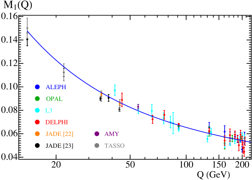
Figure -1250: Experimental data for the first moment of thrust. The solid line corresponds to the result from the first row of Tab. 4, and uses a fixed order code with power corrections in a renormalon-free scheme, but no resummation (neither QED nor bottom mass corrections).

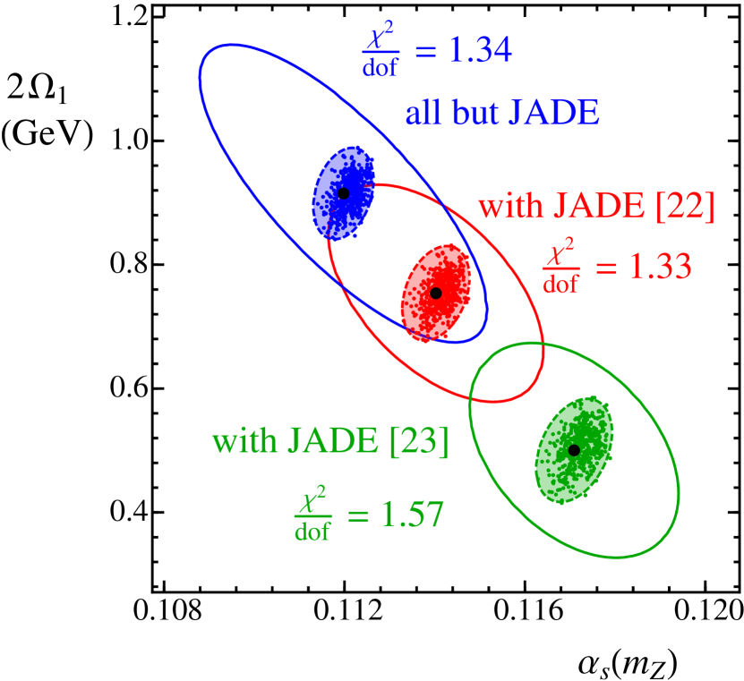
Figure -1249: Fit results when using ALEPH, DELPHI, OPAL, L3, AMY, TASSO, but no JADE data (upper blue ellipse), when also including JADE data from Ref. Movilla Fernandez et al. (1998) (red central ellipse) [ our default data set ], and when instead including the JADE data from Ref. Pahl et al. (2009a) (green lower ellipse). The ellipses here correspond to $1$-$\sigma$ for two parameters (68% CL).

VI Higher Moment Analysis

In this section we consider higher moments, $M_{n\geq 2}$, which have been measured experimentally up to $n=5$. From Eq. (II.2) we see that these moments have power corrections $\propto 1/Q^{k}$ for $k\geq 1$. Since for the perturbative moments we have $\hat{M}_{n}/\hat{M}_{n+1}\simeq 4$–$9$, we estimate that the $1/Q^{2}$ power corrections are suppressed by $9\Lambda_{\rm QCD}/Q$ which varies from $1/8$ to $1/44$ for the $Q$-values in our dataset, $Q\geq 35\,{\rm GeV}$. Hence, for the analysis in this section we can safely drop the $1/Q^{2}$ and higher power corrections and use the form

$$M_{n} =\hat{M}_{n}+\frac{2\,n\,\Omega_{1}}{Q}\,\hat{M}_{n-1}\,.$$ (50)

By using our fit results for $\alpha_{s}(m_{Z})$ and $\Omega_{1}$ from Eq. (45) we can directly make predictions for the moments $M_{2,3,4,5}$. This tests how well the theory does at calculating the perturbative contributions $\hat{M}_{2,3,4,5}$. The results for these moments are shown in Fig. -1248 and correspond to $\chi^{2}/{\rm dof}=1.3,2.5,0.8,1.1$ for $n=2,3,4,5$ respectively, indicating that our formalism does quite well at reproducing these moments. The larger $\chi^{2}/{\rm dof}$ for $n=3$ is related to a quite significant spread in the experimental data for this moment at $Q\gtrsim 190\,{\rm GeV}$. Note that we also see that the relation $M_{n}/M_{n+1}\simeq 4$–$9$ is satisfied by the experimental moments.

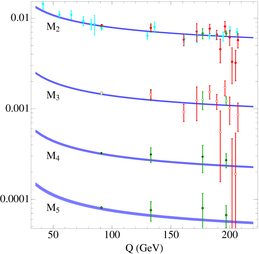
Figure -1248: Predictions for the higher moments $M_{2}$, $M_{3}$, $M_{4}$, $M_{5}$ using the best fit values from Eq. (45), and our full N³LL + ${\cal O}(\alpha_{s}^{3})$ code in the Rgap scheme, but with QED and mass effects turned off. The central points use different symbols for different moments.

An alternate way to test the higher moments is to perform a fit to this data. Since we have excluded the new JADE data in Ref. Pahl et al. (2009a), we do not have a significant dataset at smaller $Q$ values for the higher moments. With our higher moment dataset the degeneracy between $\alpha_{s}(m_{Z})$ and $\Omega_{1}$ is not broken for $n\geq 2$, and one finds very large experimental errors for a two-parameter fit already at $n=2$. However we can still fit for $\alpha_{s}(m_{Z})$ from data for each individual $M_{n\geq 2}$ by fixing the value of $\Omega_{1}$ to the best fit value in Eq. (45) from our fit to $M_{1}$. For this exercise we use our full N³LL + ${\cal O}(\alpha_{s}^{3})$ code, but with QED and mass effects turned off. The outcome is shown in Fig. -1247 and Tab. 6. We find only a little dependence of $\alpha_{s}$ on $n$, and all values are compatible with the fit to the first moment within less than 1-$\sigma$. This again confirms that our value for $\Omega_{1}$ and perturbative predictions for $\hat{M}_{n\geq 2}$ are consistent with the higher moment data.

$n$	$\alpha_{s}(m_{Z})$	$\Delta_{{\rm th}}[\alpha_{s}]$	$\Delta_{{\rm exp}}[\alpha_{s}]$	${\chi^{2}}/{{\rm dof}}$
$2$	$0.1149$	$0.0009$	$0.0005$	$1.24$
$3$	$0.1157$	$0.0009$	$0.0005$	$1.87$
$4$	$0.1151$	$0.0011$	$0.0010$	$0.39$
$5$	$0.1156$	$0.0015$	$0.0010$	$0.23$

Table 6: Numerical results for $\alpha_{s}$ from one-parameter fits to the $M_{n}$ moments. The second column gives the central values for $\alpha_{s}(m_{Z})$, the third and fourth show the theoretical and experimental errors, respectively. Since $\Omega_{1}$ was fixed for this analysis we do not quote a hadronization error.

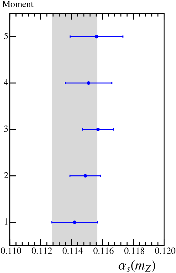
Figure -1247: One-parameter fits for $\alpha_{s}(m_{Z})$ to the first five moments. We use our full set up with power corrections and renormalon subtractions, but with QED and mass corrections turned off. The value of $\Omega_{1}$ is fixed from Eq. (45). The error bars include theoretical and experimental errors added in quadrature (not including uncertainty in $\Omega_{1}$).

In Ref. Gehrmann et al. (2010) a two-parameter fit to higher thrust moments was carried out using OPAL data and the latest low energy JADE data. For $n=2$ to $n=5$ the results increase linearly from $\alpha_{s}(m_{Z})=0.1202\pm(0.0018)_{\rm exp}\pm(0.0046)_{\rm th}$ to $\alpha_{s}(m_{Z})=0.1294\pm(0.0027)_{\rm exp}\pm(0.0070)_{\rm th}$ respectively, and the weighted average for the first five moments of thrust is $\alpha_{s}(m_{Z})\,=\,0.1208\,\pm\,0.0018_{\rm exp}\,\pm\,0.0045_{\rm th}$. The results are fully compatible within the uncertainties, and there is an indication of a trend towards larger $\alpha_{s}(m_{Z})$ extracted from higher moments. In our analysis we do not observe this trend, but our results should not be directly compared since we have only performed a one parameter fit. After further averaging over results obtained from event shapes other than thrust Ref. Gehrmann et al. (2010) obtained as their final result $\alpha_{s}(m_{Z})\,=\,0.1153\,\pm\,0.0017_{\rm exp}\,\pm\,0.0023_{\rm th}$. This is again perfectly compatible with our result in Eq. (45).

VII Higher power corrections from Cumulant Moments

In this section we use cumulant moments as defined in Eq. (27) to discuss the presence of higher power corrections and their constraints from experimental data. There are two types of power corrections that are relevant for the cumulants, those defined rigorously by QCD matrix elements which come from the leading thrust factorization theorem, $\Omega_{n}^{\prime}$, and those from our simple parameterization of higher order power corrections in Eq. (15), $\Omega_{n,j\geq 1}$. For the latter a systematic matching onto QCD matrix elements has not been carried out and the corresponding perturbative coefficients have not been determined.

For the second cumulant $M_{2}^{\prime}$ both types of power correction contribute to the leading $1/Q^{2}$ term in the combination

$$\tilde{\Omega}_{2}^{\prime} =\Omega_{2}^{\prime}+{\overline{M}}_{1,1}\,\Omega_{1,1}\,.$$ (51)

Without a calculation of the perturbative coefficient ${\overline{M}}_{1,1}$ we cannot argue that either one dominates, and hence we keep both of them. In terms of this parameter the OPE with its leading power correction for the second cumulant becomes simply

$$M_{2}^{\prime}=\hat{M}_{2}^{\prime}+\frac{4\,\tilde{\Omega}_{2}^{\prime}}{Q^{2}}\,,$$ (52)

where $\hat{M}_{2}^{\prime}$ is computed from our leading order factorization theorem, see Eq. (11). For the third cumulant $M_{3}^{\prime}$ the power correction from the leading thrust factorization theorem is $1/Q^{3}$, while that from the subleading factorization theorem is $1/Q^{2}$, so

$$M_{3}^{\prime}=\hat{M}_{3}^{\prime}+\frac{6\,{\overline{M}}_{2,1}\,\Omega_{1,1}}{Q^{2}}+\frac{8\,\Omega_{3}^{\prime}}{Q^{3}}\,.$$ (53)

where we keep both of these power corrections.

For our analysis we assume that the perturbative coefficients ${\overline{M}}_{1,1}$ and ${\overline{M}}_{2,1}$ get contributions at tree-level, and hence that their logarithmic dependence on $Q$ is $\alpha_{s}$-suppressed. Thus for fits to $M_{2}^{\prime}$ and $M_{3}^{\prime}$ we consider the three parameters $\tilde{\Omega}_{2}^{\prime}$, ${\overline{M}}_{2,1}\,\Omega_{1,1}$, and $\Omega_{3}^{\prime}$. Our theoretical expectations are that $(\Omega_{n}^{\prime})^{1/n}\sim\Lambda_{\rm QCD}$ and $(\Omega_{1,1})^{1/2}\sim(\Omega_{n}^{\prime})^{1/n}$.

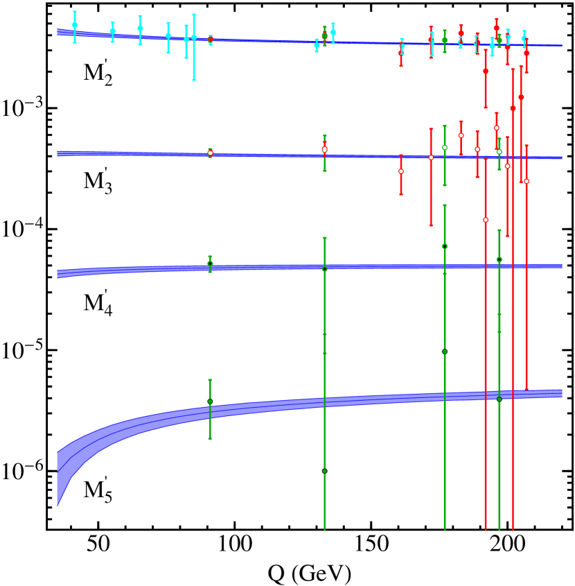
Figure -1246: Prediction of cumulants using our best-fit values for $\alpha_{s}(m_{Z})$ and $\Omega_{1}$ from the fit to the first thrust moment. The band includes only the theoretical uncertainty from the random scan. The theory prediction includes QED and mass corrections, in contrast to our numerical analysis which has no QED and $b$-mass effects and uses our default model, which translates into the following values for higher nonperturbative power corrections: $\Omega_{2}^{\prime}=\Omega_{1}^{2}/4$, $\Omega_{3}^{\prime}=\Omega_{1}^{3}/8$, $\Omega_{4}^{\prime}=3\,\Omega_{1}^{4}/32$, $\Omega_{5}^{\prime}=3\,\Omega_{1}^{5}/32$.

Since most of the experimental collaborations provide measurements only for moments we computed the cumulants using Eq. (3). To propagate the errors to the $n$-th cumulant one needs the correlations between the first $n$ moments, both statistical and systematical. Following experimental procedures we estimate the statistical correlation matrix from Monte Carlo simulations. These matrices are provided in Ref. Pahl (2007) for $Q=14,\,91.3,\,206.6\,$GeV. The computation of these matrices does not depend on the simulation of the detector and hence can be a priory employed on the data provided by any experimental collaboration. It was found that statistical correlation matrices depend very mildly on the center of mass energy, and our approach is to use the matrix computed at $14\,$GeV for $Q<60\,$GeV, the one computed at $91.3$ for $60\,{\rm GeV}\leq Q<120\,{\rm GeV}$ and the one at $206.6\,$GeV for $Q\geq 120\,$GeV. The systematic correlation matrix for the moments is estimated using the minimal overlap model based on the systematic uncertainties, and then converted to uncertainties for the cumulants. We use this method even for the few cases in which experimental collaborations provide uncertainties for the cumulants directly, since we want to treat all data on the same footing. In these cases we have checked that the results are very similar.

To some extent the prescription we employ lies in between two extreme situations: a) moments are completely uncorrelated, and b) cumulants are completely uncorrelated. Situation a) corresponds to the naive assumption that the moments are independent. Situation b) is motivated by considering that properties like the location of the peak of the distribution ($\sim M_{1}$), the width of the peak ($\sim M_{2}^{\prime}$), etc. are independent pieces of information. By assuming moments are uncorrelated one overestimates the errors of the cumulants. This would translate into larger experimental errors for our fit results and very small $\chi^{2}/{\rm dof}$. Assuming that cumulants are uncorrelated induces very strong positive correlations between moments, which then leads to small uncertainties for the cumulants, especially for the variance, and larger $\chi^{2}/{\rm dof}$ values. With the adopted prescription we use one finds a weaker positive correlation among moments, which translates into a situation between these two extremes.

	00central00	00$\Delta_{{\rm th}}$ 00	00$\Delta_{{\rm exp}}$ 00	$\frac{\chi^{2}}{{\rm dof}}$
$(\tilde{\Omega}^{\prime}_{2})^{1/2}$	$0.74\phantom{0}$	$0.09\phantom{0}$	$0.11\phantom{0}$	$0.72$
$(\Theta_{2})^{1/2}$	$1.21\phantom{0}$	$0.10\phantom{0}$	$0.22\phantom{0}$	$0.93$
$(\Theta_{3})^{1/3}$	$-2.61\phantom{0}$	$0.15\phantom{0}$	$1.51\phantom{0}$

Table 7: Determination of power corrections from fits to $M_{2}^{\prime}$ and $M_{3}^{\prime}$. All values in the table are in GeV. Columns two to four correspond to central value, theoretical uncertainty, and experimental uncertainty, respectively (the latter includes both statistical and systematic errors added in quadrature). The values displayed correspond to the linear combinations in Eq. (54), which for $M_{3}^{\prime}$ diagonalize the experimental error matrix.

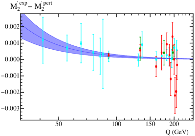
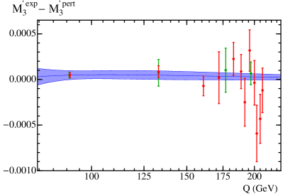
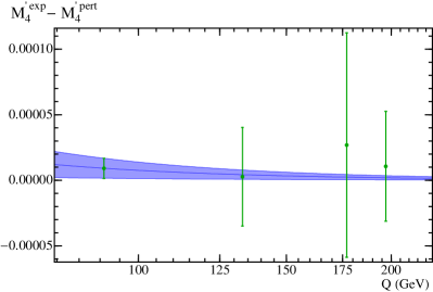
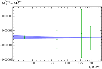
Figure -1245: Determination of power corrections from fits to data. On the vertical axes we display the $n$-th experimental cumulant with the perturbative part subtracted $M_{n}^{\prime}-{\hat{M}}_{n}^{\prime}$. The error bars shown are experimental (statistical and systematic combined) added in quadrature with perturbative errors from the random scan over the profile parameters. The top-left panel shows the fit to $\tilde{\Omega}_{2}^{\prime}/Q^{2}$, and the top-right panel shows the fit to ${\overline{M}}_{2,1}\,\Omega_{1,1}/Q^{2}$ and $\Omega_{3}^{\prime}/Q^{3}$ through the linear combinations in $\Theta_{2,3}$. The bottom two panels for $n=4,5$ show a simple fit to $\overline{M}_{3,1}\Omega_{1,1}$ and $\overline{M}_{4,1}\Omega_{1,1}$ taking $\Omega_{4}^{\prime}=\Omega_{5}^{\prime}=0$.

For our analysis we use our highest order code as described in Sec. III, and take the value $\alpha_{s}(m_{Z})=0.1142$ obtained in our fit to the first moment data with this code (see Tab. 1). Since we are analyzing cumulants $M_{n\geq 2}^{\prime}$ the value of $\Omega_{1}$ is not required, and there is no distinction between having this parameter in $\overline{\textrm{MS}}$ or the Rgap scheme. Hence in order to fit for higher power corrections we use our purely perturbative code in the $\overline{\textrm{MS}}$ scheme. Thus all of the power correction parameters extracted in this section are in the $\overline{\textrm{MS}}$ scheme. The perturbative error is estimated as in Sec. III, by a 500 point scan of theory parameters (see App. A).

Before we fit for the higher power corrections, we will check how well our factorization theorem predicts the experimental cumulants using a simple exponential model for the nonperturbative soft function (the model with only one coefficient $c_{0}=1$ from Refs. Abbate et al. (2011); Ligeti et al. (2008)). This model has higher power corrections that are determined by its one parameter $\Omega_{1}$: $\Omega_{2}^{\prime}=\Omega_{1}^{2}/4$, $\Omega_{3}^{\prime}=\Omega_{1}^{3}/8$, $\Omega_{4}^{\prime}=3\,\Omega_{1}^{4}/32$, $\Omega_{5}^{\prime}=3\,\Omega_{1}^{5}/32$. Results are shown in Fig. -1246, where good agreement between theory and data is observed.

For the $M_{n}^{\prime}$ in Fig. -1246 we also observe that $M_{n+1}^{\prime}/M_{n}^{\prime}\sim 1/10$, so the $(n+1)$-th order cumulant is generically one order of magnitude smaller than the $n$-th order cumulant.

Next we will fit for the power correction parameters $\tilde{\Omega}_{2}^{\prime}$, ${\overline{M}}_{2,1}\,\Omega_{1,1}$, and $\Omega_{3}^{\prime}$. For this analysis we neglect QED and $b$-mass effects. To facilitate this we consider the difference between the experimental cumulants $M_{n}^{\prime}$ and the perturbative theoretical cumulants $\hat{M}_{n}^{\prime}$, namely $M_{2}^{\prime}-\hat{M}_{2}^{\prime}$ and $M_{3}^{\prime}-\hat{M}_{3}^{\prime}$. From Eqs. (52) and (53) these differences are determined entirely by the power correction parameters we wish to fit. The results are shown in Tab. 7 and the upper two panels of Fig. -1245. From the $M_{2}^{\prime}-\hat{M}_{2}^{\prime}$ fit a fairly precise result is obtained for $(\tilde{\Omega}_{2}^{\prime})^{1/2}$. Its central value of $740\,{\rm MeV}$ is compatible with $\sim 2\Lambda_{\rm QCD}$, and hence agrees with naive dimensional analysis. Interestingly, we have checked that including a constant and $1/Q$ term in the second cumulant fit one finds that their coefficients are compatible with zero, in support of the theoretically expected $1/Q^{2}$-dependence.

For the fit to $M_{3}^{\prime}-\hat{M}_{3}^{\prime}$ there is a strong correlation between $\Omega_{3}^{\prime}$ and ${\overline{M}}_{2,1}\,\Omega_{1,1}$ even though they occur at different orders in $1/Q$. Since the $\chi^{2}$ is quadratic in these two parameters we can determine the linear combinations that exactly diagonalize their correlation matrix:

$$\Theta_{2} \equiv\bigg{[}\frac{6\,{\overline{M}}_{2,1}}{0.07}\bigg{]}\frac{\Omega_{1,1}}{4}+(0.3105\,{\rm GeV}^{-1})\,\Omega_{3}^{\prime}\,,$$ (54)

$$\Theta_{3} \equiv\Omega_{3}^{\prime}-(0.3105\,{\rm GeV})\,\bigg{[}\frac{6\,{\overline{M}}_{2,1}}{0.07}\bigg{]}\frac{\Omega_{1,1}}{4}\,.$$

Note that these combinations arise solely from experimental data. We have presented the coefficients of these combinations grouping together a factor of $(6{\overline{M}}_{2,1}/0.07)$, which is close to unity if $6{\overline{M}}_{2,1}\simeq\hat{M}_{1}$. The results in Tab. 7 exhibit a reasonable uncertainty for $\Theta_{2}$, but a large uncertainty for $\Theta_{3}$. Hence, at this time it is not possible to determine the original parameters $\Omega_{3}^{\prime}$ and ${\overline{M}}_{2,1}\,\Omega_{1,1}$ independently. As in the previous case, the fit does not exhibit any evidence for a $1/Q$ correction, confirming the theoretical prediction for this cumulant.

In Fig. -1245 we also show results for cumulant differences $M_{n}^{\prime}-\hat{M}_{n}^{\prime}$ versus $Q$ for $n=4$ and $n=5$. In all cases $n=2,3,4,5$ the perturbative cumulants $\hat{M}_{n}^{\prime}$ are the largest component of the cumulant moments $M_{n}^{\prime}$, as can be verified by the reduction of the values by a factor of $2$–$3$ in Fig. -1245 compared to the values in Fig. -1246. We also observe an order of magnitude suppression between the $(n+1)$’th and $n$’th terms, $(M_{n+1}^{\prime}-\hat{M}_{n+1}^{\prime})/(M_{n}^{\prime}-\hat{M}_{n}^{\prime})\sim 1/10$. For $n=4,5$ the OPE formula in Eq. (27) involves both $2^{n}\Omega_{n}^{\prime}/Q^{n}$ terms and terms with non-trivial perturbative coefficients: $(2\,n\,\overline{M}_{n-1,1}\Omega_{1,1})/Q^{2}+\ldots$ (where here the ellipses are terms at $1/Q^{3}$ and beyond). If the former dominated we would expect a suppression by $2\,\Lambda_{\rm QCD}/Q$ for the $(n+1)$’th versus $n$’th term. The observed suppression by $1/10$ is less strong and is instead consistent with domination by the $1/Q^{2}$ power correction terms in the $n=4,5$ cumulant differences. This would imply $[(n+1)\overline{M}_{n,1}]/[n\overline{M}_{n-1,1}]\sim 1/10$ and could in principle be verified by an explicit computation of these coefficients. In Fig. -1245 we show fits to a $1/Q^{2}$ power correction, which are essentially dominated by the lowest energy point at the Z-pole. The results are $\sqrt{8\,\overline{M}_{3,1}\,\Omega_{1,1}}=0.20\pm 0.08$ from fits to $M_{4}^{\prime}$ and $\sqrt{10\,\overline{M}_{4,1}\,\Omega_{1,1}}=0.07\pm 0.06$ from fits to $M_{5}^{\prime}$. These values agree with our expectation of the $\sim 1/10$ suppression between the two $\overline{M}_{n,1}$ perturbative coefficients.

In this section we have determined the $1/Q^{2}$ power correction parameter $\tilde{\Omega}_{2}^{\prime}$ with $25\%$ accuracy, and find it is $3.8\,\sigma$ different from zero. For the higher moments there are important contributions from a $\Omega_{1,1}/Q^{2}$ power correction, which appears to even dominate for $n\geq 4$. Clearly experimental data supports the pattern expected from the OPE relation in Eq. (27).

VIII Conclusions

In this work we have used a full $\tau$-distribution factorization formula developed by the authors in a previous publication Abbate et al. (2011) to study moments and cumulant moments (cumulants) of the thrust distribution. Perturbatively it incorporates $\mathcal{O}(\alpha_{s}^{3})$ matrix elements and nonsingular terms, a resummation of large logarithms, $\ln^{k}\tau$, to N³LL accuracy, and the leading QED and bottom mass corrections. It also describes the dominant nonperturbative corrections, is free of the leading renormalon ambiguity, and sums up large logs appearing in perturbative renormalon subtractions.

Theoretically there are no large logs in the perturbative expression of the thrust moments, and when normalized in the same way the perturbative result from the full $\tau$ code with resummation agrees very well with the fixed order results. Nevertheless, when the code is properly self normalized it significantly improves the order-by-order perturbative convergence towards the ${\cal O}(\alpha_{s}^{3})$ result. In particular, the results remain within the perturbative error band of the previous order, in contrast to what is observed using fixed order expressions. This lends support to the theoretical uncertainty analysis from the code with resummation.

From fits to the first moment of the thrust distribution, $M_{1}$, we find the results for $\alpha_{s}(m_{Z})$ and the leading power correction parameter $\Omega_{1}$ given in Eq. (45). They are in nice agreement with values from the fit to the tail of the thrust distribution in Ref. Abbate et al. (2011). The moment results have larger experimental uncertainties, and these dominate over theoretical uncertainties, in contrast with the situation in the tail region analysis of Ref. Abbate et al. (2011). Repeating the $M_{1}$ fit using a fixed order code with no $\ln\tau$ resummation, but still retaining the summation of large logs in the perturbative renormalon subtractions, yields fully compatible results for $\alpha_{s}(m_{Z})$ and $\Omega_{1}$.

Using a Fourier space operator product expansion we have parameterized higher order power corrections which are beyond the leading factorization formula, and analyzed the OPE both for moments $M_{n}$ and cumulants $M_{n}^{\prime}$. In the moments $M_{n}$ the $\Omega_{1}/Q$ power correction from the leading factorization theorem enters with a perturbative suppression in its coefficient, and dominates numerically over higher $1/Q$ corrections. In contrast, the cumulants $M_{n\geq 2}^{\prime}$ depend on higher order cumulant power corrections $\Omega_{n}^{\prime}/Q^{n}$ from the leading factorization theorem, and are independent of $\Omega_{1}/Q$, …, $\Omega^{\prime}_{n-1}/Q^{n-1}$. Data on these cumulants appear to indicate that they receive important contributions from a $1/Q^{2}$ power correction that enters at a level beyond the leading thrust factorization theorem. Thus the OPE reveals that cumulants are appealing quantities for exploring subleading power corrections. We performed a fit to the second cumulant and determined a non-vanishing $\tilde{\Omega}_{2}^{\prime}/Q^{2}$ power correction with a precision of $25\%$.

It would be interesting to extend the analysis performed here, based on OPE formulas related to factorization theorems, to other event shape moments and cumulants. Examples of interest include the heavy jet mass event shape Clavelli (1979); Chandramohan and Clavelli (1981); Clavelli and Wyler (1981); Catani et al. (1991); Chien and Schwartz (2010), angularities Berger et al. (2003); Hornig et al. (2009), as well as more exclusive event shapes like jet broadening Catani et al. (1992); Dokshitzer et al. (1998c); Chiu et al. (2012a); Becher et al. (2011); Chiu et al. (2012b). Other event shape moments were considered at ${\cal O}(\alpha_{s}^{3})$ in Ref. Gehrmann et al. (2010) in the context of the dispersive model for the $1/Q$ power corrections.

Appendix A Theory parameter scan

parameter	default value	range of values
$\mu_{0}$	$2$ GeV	$1.5$ to $2.5$  GeV
$n_{1}$	$5$	$2$ to $8$
$t_{2}$	$0.25$	$0.20$ to $0.30$
$e_{J}$	$0$	$-1$, $0$, $1$
$e_{H}$	$1$	$0.5$ to $2.0$
$n_{s}$	$0$	$-1$, $0$, $1$
$\Gamma^{\rm cusp}_{3}$	$1553.06$	$-1553.06$ to $+4659.18$
$j_{3}$	$0$	$-3000$ to $+3000$
$s_{3}$	$0$	$-500$ to $+500$
$\epsilon_{2}$	$0$	$-1$, $0$, $1$
$\epsilon_{3}$	$0$	$-1$, $0$, $1$

Table 8: Theory parameters relevant for estimating the theory uncertainty, their default values and range of values used for the theory scan during the fit procedure.

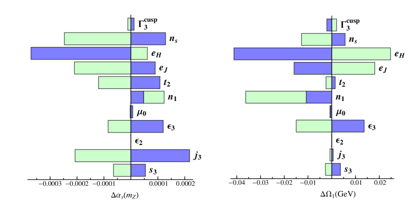
Figure -1244: Impact on parameters of the $M_{1}$ fit from variations of the best-fit values for $\alpha_{s}(m_{Z})$ and $\Omega_{1}$ values in the ranges given in Table 8. The dark shaded blue regions represent values of the parameters larger than their default values, the light shaded green regions where the parameters are smaller than their default values.

In this Appendix we describe the method we use to estimate uncertainties in our analysis. We will briefly review the profile functions and the theoretical parameters which determine the theory uncertainty. We will also describe the scan over those parameters and the effects they have on the fit results.

The profile functions used in Ref. Abbate et al. (2011), to which we refer for a more extensive description, are $\tau$-dependent factorization scales which allow us to smoothly interpolate between the theoretical constraints the hard, jet and soft scale must obey in different regions of the thrust distribution:

1) peak: $$\mu_{H}\sim Q\,,\ \ \mu_{J}\sim\sqrt{\Lambda_{\rm QCD}\,Q}\,,\ \mu_{S} \gtrsim\Lambda_{\rm QCD}\,,$$

2) tail: $$\mu_{H}\sim Q\,,\ \ \mu_{J}\sim Q\sqrt{\tau}\,,\ \mu_{S} \sim Q\,\tau\,,$$

3) far-tail: $$\mu_{H}=\mu_{J}=\mu_{S}\sim Q\,.$$ (55)

The factorization theorem derived for thrust in Ref. Abbate et al. (2011) is formally invariant under ${\cal O}(1)$ changes of the profile function scales. The residual dependence on the choice of profile functions constitutes one part of the theoretical uncertainties and provides a method to estimate higher order perturbative corrections. We adopt a set of six parameters that can be varied in our theory error analysis which encode this residual freedom while still satisfying the constraints in Eq. (A).

For the profile function at the hard scale, we adopt

$$\mu_{H}= \,e_{H}\,Q,$$ (56)

where $e_{H}$ is a free parameter which we vary from $1/2$ to $2$ in our theory error analysis.

For the soft profile function we use the form

$$\mu_{S}(\tau)=\left\{\begin{array}[]{ll}\mu_{0}+\frac{b}{2t_{1}}\tau^{2},\hskip 45.52458pt&0\leq\tau\leq t_{1},\\ b\,\tau+d,&t_{1}\leq\tau\leq t_{2},\\ \mu_{H}-\frac{b}{1-2t_{2}}(\frac{1}{2}-\tau)^{2},&t_{2}\leq\tau\leq\frac{1}{2}.\end{array}\right.$$ (60)

Here, $t_{1}$ and $t_{2}$ represent the borders between the peak, tail and far-tail regions. $\mu_{0}$ is the value of $\mu_{S}$ at $\tau=0$. Since the thrust value where the peak region ends and the tail region begins is $Q$ dependent, $t_{1}\simeq 1/Q$, we define the Q-independent parameter $n_{1}$ by $t_{1}=n_{1}/(Q/1\,\mbox{GeV})$. To ensure that $\mu_{S}(\tau)$ is a smooth function, the quadratic and linear forms are joined by demanding continuity of the function and its first derivative at $\tau=t_{1}$ and $\tau=t_{2}$, which fixes $b=2\,\big{(}\mu_{H}-\mu_{0}\big{)}/\big{(}t_{2}-t_{1}+\frac{1}{2}\big{)}$ and $d=\big{[}\mu_{0}(t_{2}+\frac{1}{2})-\mu_{H}\,t_{1}\big{]}/\big{(}t_{2}-t_{1}+\frac{1}{2}\big{)}$. In our theory error analysis we vary the free parameters $n_{1}$, $t_{2}$ and $\mu_{0}$.

The profile function for the jet scale is determined by the natural relation between the hard, jet, and soft scales

$$\mu_{J}(\tau)=\bigg{(}1+e_{J}\Big{(}\frac{1}{2}-\tau\Big{)}^{2}\bigg{)}\,\sqrt{\mu_{H}\,\mu_{S}(\tau)}\,.$$ (61)

The term involving the free ${\cal O}(1)$-parameter $e_{J}$ implements a modification to this relation and vanishes in the multijet region where $\tau=1/2$. We use a variation of $e_{J}$ to include the effect of such modifications in our estimation of the theoretical uncertainties.

In our theory error analysis we vary $\mu_{\rm ns}$ to account for our ignorance on the resummation of logarithms of $\tau$ in the nonsingular corrections. We consider three possibilities

$$\mu_{\rm ns}(\tau)=\left\{\begin{array}[]{ll}\mu_{H},\hskip 87.63454pt&n_{s}=1,\\ \mu_{J}(\tau),&n_{s}=0,\\ \frac{1}{2}[\,\mu_{J}(\tau)+\mu_{S}(\tau)\,],&n_{s}=-1.\end{array}\right.$$ (65)

The complete set of theoretical parameters and the their ranges of variation are summarized in Table 8.

Besides the parameters associated with the profile functions, the other theory parameters are $\Gamma_{3}^{\rm cusp}$, $j_{3}$, $s_{3}$, and $\epsilon_{2,3}$. The cusp anomalous dimension at $\mathcal{O}(\alpha_{s}^{4})$, $\Gamma_{3}^{\rm cusp}$ is estimated via Padé approximants and we assign a 200% uncertainty to this approximation. $j_{3}$ and $s_{3}$ represent the nonlogarithmic 3-loop term in the position-space hemisphere jet and soft functions, respectively. These two parameters and their variations are estimated via Padé approximations. The last two parameters $\epsilon_{2}$ and $\epsilon_{3}$ allow us to include the statistical errors in the numerical determination of the nonsingular distribution at two (from EVENT2 Catani and Seymour (1996, 1997)) and three (from EERAD3 Gehrmann-De Ridder et al. (2007a)) loops, respectively.

At each order we randomly scan the parameter space summarized in Table 8 with a uniform measure, extracting 500 points. Each of the points in Fig. -1254 is the result of the fit performed with a single choice of a point in the parameter space. The contour of the area in the $\alpha_{s}$-$2\,\Omega_{1}$ plane covered by the fit results at each given order is fitted to an ellipse, which is interpreted as a 1-$\sigma$ theoretical uncertainty. The ellipse is determined as follows: in a first step we determine the outermost points on the $\alpha_{s}$-$2\,\Omega_{1}$ plane (defined by the outermost convex polygon). We then perform a fit to these points using a $\chi^{2}$ which is the square of the formula for an ellipse:

$$\chi^{2}_{\rm ellipse} =\sum_{i}\big{[}a\,(\alpha_{i}-\alpha_{0})^{2}+4\,b\,(\Omega_{i}-\Omega_{0})^{2}$$ (66)

$$+\,2\,c\,(\alpha_{i}-\alpha_{0})(\Omega_{i}-\Omega_{0})\,-\,1\big{]}^{2}\,.$$

Here the sum is over the outermost points. The coordinates for the center of the ellipse, $\alpha_{0}$ and $\Omega_{0}$, are fixed ahead of time to the average of the maximum and minimum values of $\alpha_{s}(m_{Z})$ and $\Omega_{1}$ in the scan. We then minimize $\chi^{2}_{\rm ellipse}$ to determine the parameters $a,b,c$ of the ellipse.

One could further express the coefficients $a$ and $b$ by

$$a =\frac{1\,+\,\sqrt{1\,+\,4\,c^{2}\,\Delta\alpha^{2}\,\Delta\Omega^{2}}}{2\,\Delta\alpha^{2}}\,,$$ (67)

$$b =\frac{1\,+\,\sqrt{1\,+4\,\,c^{2}\,\Delta\alpha^{2}\,\Delta\Omega^{2}}}{8\,\Delta\Omega^{2}}\,,$$

where $\Delta\alpha$ and $\Delta\Omega$ are just the half of the difference of the maximum and minimum values of $\alpha_{s}(m_{Z})$ and $\Omega_{1}$, respectively, on the ellipse. Setting $\Delta\alpha$ and $\Delta\Omega$ to the corresponding values obtained from the fit points of the scan (i.e. the perturbative errors) the coefficients $a$ and $b$ can be fixed and only $c$ remains as a free parameter. The minimization of $\chi^{2}_{\rm ellipse}$ in Eq. (66) gives almost identical results regardless of whether or not Eqs. (67) are imposed.

In Fig. -1244 we vary a single parameter of Table 8 keeping all the others fixed at their respective default values, and we plot the change of $\alpha_{s}(m_{Z})$ and $\Omega_{1}$ as compared to the values obtained from the first moment thrust fit with the default setup. In the figure, the dark shaded blue area represents a variation where the parameter is larger than the default value, and the light shaded green one where the parameter is smaller. The largest uncertainty is associated with the variation of the hard scale, $e_{H}$. The value of $\alpha_{s}(m_{Z})$ is similarly affected by the uncertainty of the profile function parameters, the statistical error from the numerical determination of the 3-loop nonsingular distribution from EERAD3 Gehrmann-De Ridder et al. (2007a), and by the parameter $j_{3}$. It is rather insensitive to the variation of the 4-loop cusp anomalous dimension and the statistical error from the determination of the 2-loop nonsingular contribution to the thrust distribution. The value of $\Omega_{1}$ is mainly sensitive to the profile function parameters and $\epsilon_{3}$, but is quite insensitive to $j_{3}$.

References

- Kluth (2006) S. Kluth, Rept. Prog. Phys. 69, 1771 (2006), eprint hep-ex/0603011.
- Gehrmann-De Ridder et al. (2007a) A. Gehrmann-De Ridder, T. Gehrmann, E. W. N. Glover, and G. Heinrich, Phys. Rev. Lett. 99, 132002 (2007a), eprint 0707.1285.
- Gehrmann-De Ridder et al. (2007b) A. Gehrmann-De Ridder, T. Gehrmann, E. W. N. Glover, and G. Heinrich, JHEP 12, 094 (2007b), eprint 0711.4711.
- Weinzierl (2008) S. Weinzierl, Phys. Rev. Lett. 101, 162001 (2008), eprint 0807.3241.
- Weinzierl (2009a) S. Weinzierl, JHEP 06, 041 (2009a), eprint 0904.1077.
- Becher and Schwartz (2008) T. Becher and M. D. Schwartz, JHEP 07, 034 (2008), eprint 0803.0342.
- Chien and Schwartz (2010) Y.-T. Chien and M. D. Schwartz, JHEP 08, 058 (2010), eprint 1005.1644.
- Abbate et al. (2011) R. Abbate, M. Fickinger, A. H. Hoang, V. Mateu, and I. W. Stewart, Phys. Rev. D83, 074021 (2011), eprint 1006.3080.
- Farhi (1977) E. Farhi, Phys. Rev. Lett. 39, 1587 (1977).
- Bauer et al. (2001a) C. W. Bauer, S. Fleming, and M. E. Luke, Phys. Rev. D 63, 014006 (2001a), eprint hep-ph/0005275.
- Bauer et al. (2001b) C. W. Bauer, S. Fleming, D. Pirjol, and I. W. Stewart, Phys. Rev. D 63, 114020 (2001b), eprint hep-ph/0011336.
- Bauer and Stewart (2001) C. W. Bauer and I. W. Stewart, Phys. Lett. B 516, 134 (2001), eprint hep-ph/0107001.
- Bauer et al. (2002a) C. W. Bauer, D. Pirjol, and I. W. Stewart, Phys. Rev. D65, 054022 (2002a), eprint hep-ph/0109045.
- Bauer et al. (2002b) C. W. Bauer, S. Fleming, D. Pirjol, I. Z. Rothstein, and I. W. Stewart, Phys. Rev. D 66, 014017 (2002b), eprint hep-ph/0202088.
- Hoang and Stewart (2008) A. H. Hoang and I. W. Stewart, Phys. Lett. B660, 483 (2008), eprint 0709.3519.
- Hoang and Kluth (2008) A. H. Hoang and S. Kluth (2008), eprint 0806.3852.
- Hoang et al. (2008) A. H. Hoang, A. Jain, I. Scimemi, and I. W. Stewart, Phys. Rev. Lett. 101, 151602 (2008), eprint 0803.4214.
- Hoang et al. (2010) A. H. Hoang, A. Jain, I. Scimemi, and I. W. Stewart, Phys.Rev. D82, 011501 (2010), eprint 0908.3189.
- Bethke (2009) S. Bethke, Eur. Phys. J. C64, 689 (2009), eprint 0908.1135.
- Bethke (2012) S. Bethke, Nucl. Phys. B Proc. Supp. (to appear) (2012).
- Bethke et al. (2011) S. Bethke, A. H. Hoang, S. Kluth, J. Schieck, I. W. Stewart, et al. (2011), long author list - awaiting processing, eprint 1110.0016.
- Movilla Fernandez et al. (1998) P. A. Movilla Fernandez, O. Biebel, S. Bethke, S. Kluth, and P. Pfeifenschneider (JADE), Eur. Phys. J. C1, 461 (1998), eprint hep-ex/9708034.
- Pahl et al. (2009a) C. Pahl, S. Bethke, S. Kluth, J. Schieck, and t. J. collaboration, Eur.Phys.J. C60, 181 (2009a), eprint 0810.2933.
- Abbiendi et al. (2005) G. Abbiendi et al. (OPAL), Eur. Phys. J. C40, 287 (2005), eprint hep-ex/0503051.
- Ackerstaff et al. (1997) K. Ackerstaff et al. (OPAL), Z. Phys. C75, 193 (1997).
- Heister et al. (2004) A. Heister et al. (ALEPH), Eur. Phys. J. C35, 457 (2004).
- Abdallah et al. (2003) J. Abdallah et al. (DELPHI), Eur. Phys. J. C29, 285 (2003), eprint hep-ex/0307048.
- Abdallah et al. (2004) J. Abdallah et al. (DELPHI Collaboration), Eur.Phys.J. C37, 1 (2004), eprint hep-ex/0406011.
- Abreu et al. (1999) P. Abreu et al. (DELPHI), Phys. Lett. B456, 322 (1999).
- Acciarri et al. (2000) M. Acciarri et al. (L3 Collaboration), Phys.Lett. B489, 65 (2000), eprint hep-ex/0005045.
- Achard et al. (2004) P. Achard et al. (L3), Phys. Rept. 399, 71 (2004), eprint hep-ex/0406049.
- Braunschweig et al. (1990) W. Braunschweig et al. (TASSO), Z. Phys. C47, 187 (1990).
- Li et al. (1990) Y. K. Li et al. (AMY), Phys. Rev. D41, 2675 (1990).
- Gehrmann-De Ridder et al. (2009) A. Gehrmann-De Ridder, T. Gehrmann, E. Glover, and G. Heinrich, JHEP 0905, 106 (2009), eprint 0903.4658.
- Weinzierl (2009b) S. Weinzierl, Phys. Rev. D80, 094018 (2009b), eprint 0909.5056.
- Dokshitzer and Webber (1995) Y. L. Dokshitzer and B. R. Webber, Phys. Lett. B352, 451 (1995), eprint hep-ph/9504219.
- Akhoury and Zakharov (1995) R. Akhoury and V. I. Zakharov, Phys. Lett. B357, 646 (1995), eprint hep-ph/9504248.
- Akhoury and Zakharov (1996) R. Akhoury and V. I. Zakharov, Nucl.Phys. B465, 295 (1996), eprint hep-ph/9507253.
- Nason and Seymour (1995) P. Nason and M. H. Seymour, Nucl. Phys. B454, 291 (1995), eprint hep-ph/9506317.
- Korchemsky and Sterman (1995) G. P. Korchemsky and G. Sterman, Nucl. Phys. B437, 415 (1995), eprint hep-ph/9411211.
- Beneke (1999) M. Beneke, Phys. Rept. 317, 1 (1999), eprint hep-ph/9807443.
- Gardi (2000) E. Gardi, JHEP 0004, 030 (2000), eprint hep-ph/0003179.
- Dokshitzer et al. (1996) Y. L. Dokshitzer, G. Marchesini, and B. R. Webber, Nucl. Phys. B469, 93 (1996), eprint hep-ph/9512336.
- Dokshitzer et al. (1998a) Y. L. Dokshitzer, A. Lucenti, G. Marchesini, and G. Salam, JHEP 9805, 003 (1998a), eprint hep-ph/9802381.
- Gardi and Grunberg (1999) E. Gardi and G. Grunberg, JHEP 9911, 016 (1999), eprint hep-ph/9908458.
- Biebel (2001) O. Biebel, Phys.Rept. 340, 165 (2001).
- Pahl et al. (2009b) C. Pahl, S. Bethke, O. Biebel, S. Kluth, and J. Schieck, Eur.Phys.J. C64, 533 (2009b), eprint 0904.0786.
- Gehrmann et al. (2010) T. Gehrmann, M. Jaquier, and G. Luisoni, Eur. Phys. J. C67, 57 (2010), eprint 0911.2422.
- Dokshitzer et al. (1998b) Y. L. Dokshitzer, A. Lucenti, G. Marchesini, and G. Salam, Nucl.Phys. B511, 396 (1998b), eprint hep-ph/9707532.
- Dokshitzer and Webber (1997) Y. L. Dokshitzer and B. Webber, Phys.Lett. B404, 321 (1997), eprint hep-ph/9704298.
- Lee and Sterman (2006) C. Lee and G. Sterman (2006), eprint hep-ph/0603066.
- Lee and Sterman (2007) C. Lee and G. Sterman, Phys. Rev. D75, 014022 (2007), eprint hep-ph/0611061.
- Korchemsky and Sterman (1999) G. P. Korchemsky and G. Sterman, Nucl. Phys. B555, 335 (1999), eprint hep-ph/9902341.
- Korchemsky and Tafat (2000) G. P. Korchemsky and S. Tafat, JHEP 10, 010 (2000), eprint hep-ph/0007005.
- Ligeti et al. (2008) Z. Ligeti, I. W. Stewart, and F. J. Tackmann, Phys. Rev. D78, 114014 (2008), eprint 0807.1926.
- Lee and Stewart (2005) K. S. M. Lee and I. W. Stewart, Nucl. Phys. B721, 325 (2005), eprint hep-ph/0409045.
- Bauer et al. (2003) C. W. Bauer, M. E. Luke, and T. Mannel, Phys.Rev. D68, 094001 (2003), eprint hep-ph/0102089.
- Bauer et al. (2002c) C. W. Bauer, M. Luke, and T. Mannel, Phys.Lett. B543, 261 (2002c), eprint hep-ph/0205150.
- Leibovich et al. (2002) A. K. Leibovich, Z. Ligeti, and M. B. Wise, Phys.Lett. B539, 242 (2002), eprint hep-ph/0205148.
- Bosch et al. (2004) S. W. Bosch, M. Neubert, and G. Paz, JHEP 0411, 073 (2004), eprint hep-ph/0409115.
- Beneke et al. (2005) M. Beneke, F. Campanario, T. Mannel, and B. Pecjak, JHEP 0506, 071 (2005), eprint hep-ph/0411395.
- Kelley et al. (2011) R. Kelley, M. D. Schwartz, R. M. Schabinger, and H. X. Zhu, Phys.Rev. D84, 045022 (2011), eprint 1105.3676.
- Hornig et al. (2011) A. Hornig, C. Lee, I. W. Stewart, J. R. Walsh, and S. Zuberi, JHEP 1108, 054 (2011), eprint 1105.4628.
- Monni et al. (2011) P. F. Monni, T. Gehrmann, and G. Luisoni, JHEP 1108, 010 (2011), eprint 1105.4560.
- Pahl (2007) C. Pahl, Ph.D. thesis, TU Munich (2007).
- Clavelli (1979) L. Clavelli, Phys.Lett. B85, 111 (1979).
- Chandramohan and Clavelli (1981) T. Chandramohan and L. Clavelli, Nucl.Phys. B184, 365 (1981).
- Clavelli and Wyler (1981) L. Clavelli and D. Wyler, Phys.Lett. B103, 383 (1981).
- Catani et al. (1991) S. Catani, G. Turnock, and B. Webber, Phys.Lett. B272, 368 (1991).
- Berger et al. (2003) C. F. Berger, T. Kúcs, and G. Sterman, Phys. Rev. D 68, 014012 (2003), eprint hep-ph/0303051.
- Hornig et al. (2009) A. Hornig, C. Lee, and G. Ovanesyan, JHEP 05, 122 (2009), eprint 0901.3780.
- Catani et al. (1992) S. Catani, G. Turnock, and B. Webber, Phys.Lett. B295, 269 (1992).
- Dokshitzer et al. (1998c) Y. L. Dokshitzer, A. Lucenti, G. Marchesini, and G. Salam, JHEP 9801, 011 (1998c), eprint hep-ph/9801324.
- Chiu et al. (2012a) J.-y. Chiu, A. Jain, D. Neill, and I. Z. Rothstein, Phys.Rev.Lett. 108, 151601 (2012a), eprint 1104.0881.
- Becher et al. (2011) T. Becher, G. Bell, and M. Neubert, Phys.Lett. B704, 276 (2011), 15 pages, 4 figures, eprint 1104.4108.
- Chiu et al. (2012b) J.-Y. Chiu, A. Jain, D. Neill, and I. Z. Rothstein, JHEP 1205, 084 (2012b), eprint 1202.0814.
- Catani and Seymour (1996) S. Catani and M. H. Seymour, Phys. Lett. B378, 287 (1996), eprint hep-ph/9602277.
- Catani and Seymour (1997) S. Catani and M. H. Seymour, Nucl. Phys. B485, 291 (1997), eprint hep-ph/9605323.