Fractionalizing Majorana fermions: non-abelian statistics on the edges of abelian quantum Hall states

Abstract

We study the non-abelian statistics characterizing systems where counter-propagating gapless modes on the edges of fractional quantum Hall states are gapped by proximity-coupling to superconductors and ferromagnets. The most transparent example is that of a fractional quantum spin Hall state, in which electrons of one spin direction occupy a fractional quantum Hall state of $\nu=1/m$, while electrons of the opposite spin occupy a similar state with $\nu=-1/m$. However, we also propose other examples of such systems, which are easier to realize experimentally. We find that each interface between a region on the edge coupled to a superconductor and a region coupled to a ferromagnet corresponds to a non-abelian anyon of quantum dimension $\sqrt{2m}$. We calculate the unitary transformations that are associated with braiding of these anyons, and show that they are able to realize a richer set of non-abelian representations of the braid group than the set realized by non-abelian anyons based on Majorana fermions. We carry out this calculation both explicitly and by applying general considerations. Finally, we show that topological manipulations with these anyons cannot realize universal quantum computation.

I Introduction

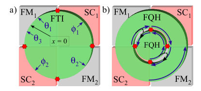
Figure 1: Schematic setup. (a) A fractional topological insulator (FTI) realization. A FTI droplet with an odd filling factor $1/m$ is proximity coupled to ferromagnets (FM) and to superconductors (SC), which gap out its edge modes. The interfaces between the SC and FM segments on the edge of the FTI are marked by red stars. (b) A fractional quantum Hall (FQH) realization. A FQH droplet with filling factor $1/m$ is separated by a thin barrier into two pieces: an inner disk, and an outer annulus. On either side of the barrier, there are counter-propagating edge states, which are proximity coupled to superconductors and ferromagnets.

Recent years have witnessed an extensive search for electronic systems in which excitations (“quasi-particles”) follow non-abelian quantum statistics. In such systems, the presence of quasi-particles, also known as “non-abelian anyons” Leinaas and Myrheim (1977); Blok and Wen (1992); Stern (2010), makes the ground state degenerate. A mutual adiabatic interchange of quasi-particles’ positionsArovas et al. (1984) implements a unitary transformation that operates within the subspace of ground states, and shifts the system from one ground state to another. Remarkably, this unitary transformation depends only on the topology of the interchange, and is insensitive to imprecision and noise. These properties make non-abelian anyons a test-ground for the idea of topological quantum computationKitaev (2003). The search for non-abelian systems originated from the Moore-Read theory Moore and Read (1991) for the $\nu=5/2$ Fractional Quantum Hall (FQH) state, and went on to consider other quantum Hall states Read and Rezayi (1996); Stern (2008), spin systems Kitaev (2006), $p$-wave superconductors Read and Green (2000); Ivanov (2001); Nayak and Wilczek (1996), topological insulators in proximity coupling to superconductors Fu and Kane (2008, 2009) and hybrid systems of superconductors coupled to semiconductors where spin-orbit coupling is strong Sau et al. (2010a); Qi et al. (2010); Sau et al. (2010b); Stanescu et al. (2010); Oreg et al. (2010); Lutchyn et al. (2010); Cook and Franz (2011). Signatures of Majorana zero modes may have been observed in recent experiments Mourik et al. (2012); Willett et al. (2009); An et al. ; Rokhinson et al. ; Das et al. .

In the realizations based on superconductors, whether directly or by proximity, the non-abelian statistics results from the occurrence of zero-energy Majorana fermions bound to the cores of vortices or to the ends of one dimensional wires Read and Green (2000); Ivanov (2001); Nayak and Wilczek (1996); Fu and Kane (2008, 2009); Sau et al. (2010a); Qi et al. (2010); Sau et al. (2010b); Stanescu et al. (2010); Oreg et al. (2010); Lutchyn et al. (2010); Cook and Franz (2011); Alicea (2012); Beenakker (2011). Majorana-based non-abelian statistics is, from the theory side, the most solid prediction for the occurrence of non-abelian statistics, since it is primarily based on the well tested BCS mean field theory of superconductivity. Moreover, from the experimental side it is the easiest realization to observeMourik et al. (2012). The set of unitary transformations that may be carried out on Majorana-based systems is, however, rather limited, and does not allow for universal topological quantum computation Nayak et al. (2008); Freedman et al. (2002).

In this work we introduce and analyze a non-abelian system that is based on proximity coupling to a superconductor but goes beyond the Majorana fermion paradigm. The system we analyze is based on the proximity-coupling of fractional quantum Hall systems or fractional quantum spin Hall systems Levin and Stern (2009) to superconductors and ferromagnetic insulators (we will use the terms “fractional topological insulators” and “fractional quantum spin Hall states” interchangeably). The starting point of our approach is the following observation, made by Fu and Kane Fu and Kane (2009) when considering the edge states of two-dimensional (2D) topological insulators of non-interacting electrons, of which the integer quantum spin Hall state Kane and Mele (2005); Bernevig and Zhang (2006) is a particular example: In a 2D topological insulator, the gapless edge modes may be gapped either by breaking time reversal symmetry or by breaking charge conservation along the edge. The former may be broken by proximity coupling to a ferromagnet, while the latter may be broken by proximity coupling to a superconductor. Remarkably, there must be a single Majorana mode localized at each interface between a region where the edge modes are gapped by a superconductor to a region where the edge modes are gapped by a ferromagnet.

Our focus is on similar situations in cases where the gapless edge modes are of fractional nature. We find that under these circumstances, the Majorana operators carried by the interfaces in the integer case are replaced by “fractional Majorana operators” whose properties we study.

We consider three types of physical systems. The first (shown schematically in Fig. 1a) is that of a 2D fractional topological insulatorLevin and Stern (2009), that may be viewed as a 2D system in which electrons of spin-up form an FQH state of a Laughlin Laughlin (1983) fraction $\nu=1/m$ , with $m$ being an odd integer, and electrons of spin-down form an FQH state of a Laughlin fraction $\nu=-1/m$.

The second system (1b) is a Laughlin FQH droplet of $\nu=1/m$, divided by a thin insulating barrier into an inner disk and an outer annulus. On the inner disk, the electronic spins are polarized parallel to the magnetic field (spin-up), and on the annulus the electronic spins are polarized anti-parallel to the magnetic field (spin-down). Consequently, two edge modes flow on the two sides of the barrier, with opposite spins and opposite velocities. Such a state may be created under circumstances where the sign of the $g$-factor is made to vary across the barrier.

The third system is an electron-hole bi-layer subjected to a perpendicular magnetic field, in which one layer is tuned to an electron spin-polarized filling factor of $\nu=1/m$, and the other to a hole spin-polarized $\nu=1/m$ state. In particular, this may be realized in a material with a spectrum that is electron-hole symmetric, such as graphene.

In all these cases, the gapless edge mode may be gapped either by proximity coupling to a superconductor or by proximity coupling to a ferromagnet. We imagine that the edge region is divided into $2N$ segments, where the superconducting segments are all proximity coupled to the same bulk superconductor, and the ferromagnetic segments are all proximity coupled to the same ferromegnet. The length of each segment is large compared to the microscopic lengths, so that tunneling between neighboring SC-FM interfaces is suppressed. We consider the proximity interactions of the segments with the superconductor and the ferromegnet to be strong.

The questions we ask ourselves are motivated by the analogy with the non-interacting systems of Majorana fermions: what is the degeneracy of the ground state? Is this degeneracy topologically protected? What is the nature of the degenerate ground states? And how can one manipulate the system such that it evolves, in a protected way, between different ground states?

The structure of the paper is as follows: In Sec. II we give the physical picture that we developed, and summarize our results. In Sec. III we define the Hamiltonian of the system. In Sec. IV we calculate the ground state degeneracy. In Sec. V we define the operators that are localized at the interfaces, and act on the zero energy subspace. In Sec. VI we calculate in detail the unitary transformation that corresponds to a braid operation. In Sec. VII we show how this transformation may be deduced from general considerations, bypassing the need for a detailed calculation. In Sec. VIII we discuss several aspects of the fractionalized Majorana operators, and their suitability for topological quantum computation. Sec. IX contains some concluding remarks. The paper is followed by appendices which discuss several technical details.

II The physical picture and summary of the results

There are three types of regions in the systems we consider: the bulk, the parts of the edge that are proximity-coupled to a superconductor, and the parts of the edge that are proximity-coupled to a ferromagnet.

The bulk is either a fractional quantum Hall state or a fractional quantum spin Hall state. In both cases it is gapped and incompressible, and its elementary excitations are localized quasi-particles whose charge is a multiple of $e^{*}=e/m$ electron charges. In our analysis we will assume that the area enclosed by the edge modes encloses $n_{\uparrow}$ quasi-particles of spin-up and $n_{\downarrow}$ quasi-particles of spin down. These quasi-particles are assumed to be immobile.

In the parts of the edge that are coupled to a superconductor the charge is defined only modulo $2e$, because Cooper-pairs may be exchanged with the superconductor. Thus, the proper operator to describe the charge on a region of this type is $e^{i\pi\hat{Q}_{i}}$, with $\hat{Q}_{i}$ being the charge in $i$’th superconducting region. Since the superconducting region may exchange $e^{*}$ charges with the bulk, these operators may take the values $e^{i\pi q_{i}/m}$, with $q_{i}$ an integer whose value is between zero and $2m-1$. The pairing interaction leads to a ground state that is a spin singlet, and thus the expectation value of the spin within each superconducting region vanishes. As we show below, the Hamiltonian of the system commutes with the operators $e^{i\pi\hat{Q}_{i}}$ in the limit we consider. For the familiar $m=1$ case, these operators measure the parity of the number of electrons within each superconducting region.

The edge regions that are proximity-coupled to ferromagnets are, in some sense, the dual of the superconducting regions. The ferromagnet introduces back-scattering between the two counter-propagating edge modes, leading to the formation of an energy gap. If the chemical potential lies within this gap, the region becomes insulating and incompressible. Consequently, the charge in the region does not fluctuate, and its value may be defined as zero. The spin, on the other hand, does fluctuate. Since the back-scattering from spin up electron to spin down electron changes the total spin of the region by two (where the electronic spin is defined as one unit of spin), the operator that may be expected to have an expectation value within the ground state is $e^{i\pi\hat{S}_{i}}$, with $\hat{S}_{i}$ being the total spin in the $i$’th ferromagnet region. Again, spins of $1/m$ may be exchanged with the bulk, and thus these operators may take the eigenvalues $e^{i\pi s_{i}/m}$, with $s$ an integer between zero and $2m-1$. The Hamiltonian of the system commutes with the operators $e^{i\pi\hat{S}_{i}}$ in the limit we consider.

The operators $e^{i\pi\hat{Q}_{i}}$ and $e^{i\pi\hat{S}_{i}}$ label the different domains in the system, as indicated in Fig 2a. They satisfy a constraint dictated by the state of the bulk,

$$\prod_{i=1}^{N}e^{i\pi\hat{Q}_{i}}=e^{i\pi(n_{\uparrow}+n_{\downarrow})/m}$$

$$\prod_{i=1}^{N}e^{i\pi\hat{S}_{i}}=e^{i\pi(n_{\uparrow}-n_{\downarrow})/m}$$ (1)

For the familiar $m=1$ case there are only two possible solutions for these constraints, corresponding to the two right hand sides of Eq. (1) being both $+1$ or both $-1$. For a general $m$, the number of topologically distinct constraints is $2m^{2}$, since Eqs. (1) are invariant under the transformation where $n_{\uparrow}\rightarrow n_{\uparrow}\pm m$ together with $n_{\downarrow}\rightarrow n_{\downarrow}\pm m$. These sets may be spanned by the values $0\leq n_{\uparrow}\leq 2m-1$ and $0\leq n_{\downarrow}\leq m-1$.

The degeneracy of the ground state may be understood by examining the algebra constructed by the operators $e^{i\pi\hat{Q}_{i}}$ and $e^{i\pi\hat{S}_{i}}$. As we show in the next section, the operators $e^{i\pi\hat{S}_{i}},e^{i\pi{\hat{Q}}_{i}}$ satisfy

$$[e^{i\pi{\hat{Q}}_{i}},e^{i\pi{\hat{Q}}_{j}}] = [e^{i\pi{\hat{S}}_{i}},e^{i\pi{\hat{S}}_{j}}]=0,$$

$$\left[e^{i\pi{\hat{Q}_{j}}},\prod_{i=1}^{N}e^{i\pi\hat{S}_{i}}\right] = \left[e^{i\pi{\hat{S}_{j}}},\prod_{i=1}^{N}e^{i\pi\hat{Q}_{i}}\right]=0,$$

$$e^{i\pi\hat{Q}_{j}}e^{i\pi{\sum_{k=1}^{l}\hat{S}}_{k}} = e^{i\frac{\pi}{m}\delta_{jl}}e^{i\pi{\sum_{k=1}^{l}\hat{S}}_{k}}e^{i\pi\hat{Q}_{j}},$$ (2)

where, in the last equation, $1\leq j,l<N$ (see Fig 2a for the enumeration convention). As manifested by Eqs. (2), the pairs of operators $e^{i\pi\hat{Q}_{i}},e^{i\pi{\sum_{k=1}^{i}\hat{S}}_{k}}$ form $N-1$ pairs of degrees of freedom, where members of different pairs commute with one another. It is the relation between members of the same pairs, expressed in Eq. (2), from which the ground state degeneracy may be easily read out. As is evident from this equation, if $|\psi\rangle$ is a ground state of the system which is also an eigenstate of $e^{i\pi\hat{Q}_{j}}$, then $2m-1$ additional ground are $\left(e^{i\pi\sum_{i=1}^{j}\hat{S}_{i}}\right)^{k}|\psi\rangle$, where $k$ is an integer between $1$ and $2m-1$. With $N-1$ mutually independent pairs, we reach the conclusion that the ground state degeneracy, for a given value of $n_{\uparrow},n_{\downarrow}$, is $(2m)^{N-1}$.

The operators acting within a sector of given $n_{\uparrow}$, $n_{\downarrow}$ of the ground state subspace are represented by $(2m)^{N-1}\times(2m)^{N-1}$ matrices. They may be expressed in terms of sums and products of the operators appearing in (2). The physical operations described by the operators $e^{i\pi\hat{S}_{i}},e^{i\pi{\hat{Q}}_{i}}$ can also be read off the relations (2). The operator $e^{i\pi\hat{S}_{i}}$ transfers a quasi-particle of charge $e/m$ from the $i-1$’th superconductor to the $i$’th superconductor. Since the spin within the superconductor vanishes, there is no distinction, within the ground state manifold, between the possible spin states of the transferred quasi-particle. In contrast, the operator $e^{i\pi\sigma\hat{Q}_{i}}$ transfers a quasi-particle of spin $\sigma=\pm 1$ across the $i$’th superconductor.

For $m=1$ the operators $e^{i\pi\hat{S}_{i}}$ and $e^{i\pi\hat{Q}_{i}}$, measuring the parity of the spin and the charge in the $i$’th ferromagnetic and superconducting region, respectively, may be expressed in terms of Majorana operators that reside at the interfaces bordering that region. A similar representation exists also in the case of $m\neq 1$. Its details are given in Section V.

We stress that the ground state degeneracy is topological, in the sense that no measurement of a local operator can determine the state of the system within the ground state subspace. For $m=1$, this corresponds to the well-known “topological protection” of the ground state subspace of Majorana fermions Nayak et al. (2008); Stern et al. (2004), as long as single electron tunneling is forbidden either between the different Majorana modes, or between the Majorana modes and the external world. In the fractional case the states in the ground state manifold can be labelled by the fractional part of the spin or charge of the FM/SC segments, respectively. These clearly cannot be measured locally. Moreover, they can only change by tunneling fractional quasi-particles between different segments; even tunneling electrons from the outside environment cannot split the degeneracy completely, because it can only change the charge and spin of the system by integers.

Topological manipulations of non-abelian anyons confined to one dimension are somewhat more complicated than those carried out in two dimensions. The simplest manipulation does not involve any motion of the anyons, but rather involves either a $2\pi$ twist of the order parameter of the superconductor coupled to one or several superconducting segments, or a $2\pi$ rotation of the direction of the magnetization of the ferromagnet coupled to the insulating segmentsTeo and Kane (2010). When a vortex encircles the $i$’th superconducting region it leads to the accumulation of a Berry phase of $2\pi$ multiplied by the number of Cooper-pairs it encircles. In the problem we consider, this phase amounts to $e^{i\pi\hat{Q}_{i}}$, and that is the unitary transformation applied by such rotation. As explained above, this transformation transfers a spin of $1/m$ between the two ferromagnetic regions with which the superconductor borders. Similarly, a rotation of the magnetization in the ferromagnetic region leads to a transfer of a charge of $e/m$ between the two superconductors with which the ferromagnet borders.

A more complicated manipulation is that of anyons’ braiding, and its associated non-abelian statistics. While in two dimensions the braiding of anyons is defined in terms of world lines ${\bf R}(t)$ that braid one another as time evolves, in one dimension - both in the integer $m=1$ and in the fractional case - a braiding operation requires the introduction of tunneling terms between different points along the edgeAlicea et al. (2011); Sau et al. (2011). The braiding is then defined in terms of trajectories in parameter space, which includes the tunneling amplitudes that are introduced to implement the braiding. The braiding is topological in the sense that it does not depend on the precise details of the trajectory that implements it, as long as the degeneracy of the ground state manifold does not vary throughout the implementation. Physically, one can imagine realizing such operations by changing external gate potentials which deform the shape of the system’s edge adiabatically (similar to the operations proposed for the Majorana case Alicea et al. (2011); Halperin et al. (2012)).

In the integer $m=1$ case, the interchange of two anyons positioned at two neighboring interfaces is carried out by subjecting the system to an adiabatically time dependent Hamiltonian in which interfaces are coupled to one another. When two or three interfaces are coupled to one another, the degeneracy of the ground state does not depend on the precise value of the couplings, as long as they do not all vanish at once. Consequently, one may “copy” an anyon $a$ onto an anyon $c$ by starting with a situation where corresponding interfaces $b$ and $c$ are tunnel coupled, and then turning on a coupling between $a$ and $b$ while simultaneously turning off the coupling of $b$ to $c$. Three consecutive “copying” processes then lead to an interchange, and the resulting interchanges generate a non-abelian representation of the braid group.

In the integer case only electrons may tunnel between two interfaces, thus allowing us to characterize the tunneling term by one tunneling amplitude. In contrast, in the fractional case more types of tunneling processes are possible, corresponding to the tunneling of any number of quasi-particles of charges $e/m$ and spin $\pm 1/m$. To define the effective Hamiltonian coupling two interfaces, we need to specify the amplitudes for all these distinct processes. As one may expect, if only electrons are allowed to tunnel between the interfaces (as may be the case if the tunneling is constrained to take place through the vacuum), the $m=1$ case is reproduced. When single quasi-particles of one spin direction are allowed to tunnel (which is the natural case for the FQHE realization of our model), tunnel coupling between either two or three interfaces reduces the degeneracy of the ground state by a factor of $2m$. This case then opens the way for interchanges of the positions of anyons by the same method envisioned for the integer case. We analyze these interchanges in detail below.

Our analysis of the unitary transformations that correspond to braiding schemes goes follows different routes. In the first, detailed in Section VI, we explicitly calculate these transformation for a particular case of anyons interchange. In the second, detailed in Section VII, we utilize general properties of anyons to find all non-abelian representations of the braid group that satisfy conditions that we impose, which are natural to expect from the system we analyze. Both routes indeed converge to the same result. While the details of the calculations are given in the following sections, here we discuss their results.

To consider braiding, we imagine that two anyons at the two ends of the $i$’th superconducting region are interchanged. For the $m=1$ case the interchange of two Majorana fermions correspond to the transformation

$$\frac{1}{\sqrt{2}}\left[1\pm i\exp(i\pi\hat{Q}_{i})\right].$$ (3)

This transformation may be written as $\exp[i\frac{\pi}{2}(\hat{Q}_{i}-k)^{2}]$ with $k=0,1$ corresponding to the $\pm$ sign in (3), or as $\frac{1}{\sqrt{2}}\left(1\pm\gamma_{1}\gamma_{2}\right)$, with $\gamma_{1},\gamma_{2}$ the two localized Majorana modes at the two ends of the superconducting region. Its square is the parity of the charge in the superconducting region, and its fourth power is unity. Note that in two dimensions, the two signs in (3) correspond to anyons exchange in clockwise and anti-clockwise sense. In contrast, in one dimension the two signs may be realized by different choices of tunneling amplitudes, and are not necessarily associated with a geometric notion. Consistent with the topological nature of the transformation, a trajectory that leads to one sign in (3) cannot be deformed into a trajectory that corresponds to a different sign, without passing through a trajectory in which the degeneracy of the ground state varies during the execution of the braiding.

Guided by this familiar example, we expect that at the fractional case the unitary transformation corresponding to this interchange will depend only on $e^{i\pi\hat{Q}_{i}}$. We expect to be able to write it as

$$U(\hat{Q}_{i})=\sum_{j=0}^{2m-1}a_{j}\exp{\left(i\pi j\hat{Q}_{i}\right)},$$ (4)

with some complex coefficients $a_{j}$, i.e., to be periodic in $\hat{Q}_{i}$, with the period being $2$. We expect the values of $a_{j}$ to depend on the type of tunneling amplitudes that are used to implement the braiding.

In our analysis, we find a more compact, yet equivalent, form for the transformation $U$, which is

$$U(\hat{Q}_{i})=e^{i\alpha\pi\left(\hat{Q}_{i}-\frac{k}{m}\right)^{2}}.$$ (5)

The value of $\alpha$ depends on the type of particle which tunnels during the implementation of the braiding, while the value of $k$ depends on the value of the tunneling amplitudes. For an electron tunneling, $\alpha=\frac{m^{2}}{2}$. Just as for the $m=1$ case, for this value of $\alpha$ the unitary transformation (5) has two possible eigenvalues, $U^{4}=1$, and it is periodic in $k$ with a period of $2$. For braiding carried out by tunneling single quasi-particles we find $\alpha=\frac{m}{2}$. In this case $U^{4m}=1$, and $U$ is periodic in $k$ with a period of $2m$.

Just as in the $m=1$ case, trajectories in parameter space that differ by their value of $k$ are separated by trajectories that involve a variation in the degeneracy of the ground state. We note that up to an unimportant abelian phase, the unitary transformation (5) may be thought of as composed of a transformation $e^{i\alpha\pi\hat{Q}_{i}^{2}}$ that results from an interchange of anyons, multiplied by a transformation $e^{\frac{2\alpha\pi i}{m}\hat{Q}_{i}k}$ that results from a vortex encircling the $i$’th superconducting region $2\alpha k/m$ times.

Non-abelian statistics is the cornerstone of topological quantum computation Nayak et al. (2008); Kitaev (2003), due to possibility it opens for the implementation of unitary transformations that are topologically protected from decoherence and noise. It is then natural to examine whether the non-abelian anyons that we study allow for universal quantum computation, that is, whether any unitary transformation within the ground state subspace may be approximated by topological manipulations of the anyons Freedman et al. (2002). We find that, at least for unitary time evolution (i.e., processes that do not involve measurements) the answer to this question is negative, as it is for the integer case.

III Edge model

The edge states of a FTI are described by a hydrodynamic bosonized theory Wen (1990); Lee and Wen (1991). The edge effective Hamiltonian is written as

$$H =\frac{mu}{2\pi}\int dx\left[K\left(x\right)\left(\partial_{x}\phi\right)^{2}+\frac{1}{K\left(x\right)}\left(\partial_{x}\theta\right)^{2}\right]$$

$$-\int dx\left[g_{S}\left(x\right)\cos\left(2m\phi\right)+g_{F}\left(x\right)\cos\left(2m\theta\right)\right].$$ (6)

Here, $u$ is the edge mode velocity, $\phi$, $\theta$ are bosonic fields satisfying the commutation relation $\left[\phi\left(x\right),\theta\left(x^{\prime}\right)\right]=\frac{i\pi}{m}\Theta\left(x^{\prime}-x\right)$ where $\Theta$ is the Heaviside step function, and $g_{S}\left(x\right)$, $g_{F}\left(x\right)$ describe position-dependent proximity couplings to a SC and a FM, which we take to be constant in the SC/FM regions and zero elsewhere, respectively. The magnetization of the FM is taken to be in the $x$ direction. $K\left(x\right)$ is a space-dependent Luttinger parameter, originating from interactions between electrons of opposite spins. The charge and spin densities are given by $\rho=\partial_{x}\theta/\pi$ and $s^{z}=\partial_{x}\phi/\pi$, respectively (where the spin is measured in units of the electron spin $\hbar/2$). A right or left moving electron is described by the operators $\psi_{\pm}=e^{im\left(\phi\pm\theta\right)}$.

Crucially for the arguments below, we will assume that the entire edge is gapped by the proximity to the SC and FM, except (possibly) the SC/FM interface. This can be achieved, in principle, by making the proximity coupling to the SC and FM sufficiently strong.

IV Ground state degeneracy of disk with 2N segments

We consider a disk with $2N$ FM/SC interfaces on its boundary (illustrated in Fig. 1a for $N=2$). In order to determine the dimension of the ground state manifold, we construct a set of commuting operators, which can be used to characterize the ground states. Consider the operators: $e^{i\pi Q_{j}}\equiv e^{i\left(\theta_{j+1}-\theta_{j}\right)}$, $j=1,\dots,N$, where $\theta_{j}$ is a $\theta$ field evaluated at an arbitrary point near the middle of the $j$th FM region. The origin ($x=0$) is chosen to lie within the first FM region (see Fig. 1a). The operator $\theta_{N+1}$ is located within this region, to the left of the origin ($x<0$), while $\theta_{1}$ is to the right of the origin ($x>0$). The fields $\theta$, $\phi$ satisfy the boundary conditions $e^{i\pi Q_{\mathrm{tot}}}=e^{i\left[\theta(L^{-})-\theta(0^{+})\right]}$ and $e^{i\pi S_{\mathrm{tot}}}=e^{i\left[\phi(L^{-})-\phi(0^{+})\right]}$, where $L$ is the perimeter of the system, and $Q_{\mathrm{tot}}$, $S_{\mathrm{tot}}$ are the total charge and spin on the edge, respectively.

Since we are in the gapped phase of the sine-Gordon model of Eq. (6), we expect in the thermodynamic limit (where the size of all of the segments becomes large) that the $\theta$ field is essentially pinned to the minima of the cosine potential in the FM regions. (Similar considerations hold for the $\phi$ fields in the SC regions.) In other words, the $\theta\rightarrow\theta+\pi/m$ symmetry is spontaneously broken. In this phase, correlations of the fluctuations of $\theta$ decay exponentially on length scales larger than the correlation length $\xi\sim u/\Delta_{F}$, where $\Delta_{F}$ is the gap in the FM regions (see Appendix A for an analysis of the gapped phase). Therefore, one can construct approximate ground states which are characterized by $\langle e^{i(\theta_{j+1}-\theta_{j})}\rangle=\langle e^{i\pi Q_{j}}\rangle\equiv\lambda_{j}\neq 0$, where $\lambda_{j}=\left|\lambda\right|e^{\frac{i\pi}{m}q_{j}}$, where $q_{j}\in\left\{0,\dots,2m-1\right\}$ can be chosen independently for each FM domain. The energy splitting between these ground states is suppressed in the thermodynamic limit as $e^{-R/\xi}$, where $R$ is the length each region, as discussed below and in Appendix A.

In addition, $e^{i\pi S_{\mathrm{tot}}}$ commutes both with the Hamiltonain and with $e^{i\pi Q_{j}}$. Therefore the ground states can be chosen to be eigenstates of $e^{i\pi S_{\mathrm{tot}}}$, with eigenvalues $e^{i\frac{\pi}{m}s}$, $s\in\left\{0,\dots,2m-1\right\}$. We label the approximate ground states as $|\left\{q\right\};s\rangle\equiv|q_{1},\dots,q_{N};s\rangle$, where $|\left\{q\right\};s\rangle$ satisfies that $\langle\left\{q\right\};s|e^{i\pi Q_{j}}|\left\{q\right\};s\rangle=\left|\lambda\right|e^{\frac{i\pi}{m}q_{j}}$.

For a large but finite system, the $|\{q\};s\rangle$ states are not exactly degenerate. There are two effects that lift the degeneracy between them: intra-segment instanton tunneling events between states with different $\{q\}$, and inter-segment “Josephson” couplings which make the energy dependent on the values of $\{q\}$. However, both of these effects are suppressed exponentially as $e^{-R/\xi}$, as they are associated with an action which grows linearly with the system size. Therefore, we argue that $|\{q\};s\rangle$ are approximately degenerate, up to exponentially small corrections, for any choice of the set $\{q\},s$.

Similarly, one can define a set of “dual” operators $e^{i\pi S_{j}}\equiv e^{i\left(\phi_{j}-\phi_{j-1}\right)}$, $j=2,\dots,N$, and $e^{i\pi S_{1}}=e^{i\pi S_{\mathrm{tot}}}\prod^{N}_{i=2}e^{-i\pi S_{i}}$. Although the SC regions are in the gapped phase, and the fields $\phi_{j}$ are pinned near the minima of the corresponding cosine potentials, note that the approximate ground states $|\left\{q\right\};s\rangle$ cannot be further distinguished by the expectation values of the operators $e^{i\pi S_{j}}$. In fact, these states satisfy $\langle\{q\};s|e^{i\pi S_{j}}|\{q\};s\rangle\rightarrow 0$ in the thermodynamic limit. That is because the operators $e^{i\pi S_{j}}$ and $e^{i\pi Q_{j}}$ satisfy the commutation relations

$$e^{i\pi S_{i}}e^{i\pi Q_{j}}=e^{\frac{i\pi}{m}\left(\delta_{i,j+1}-\delta_{i,j}\right)}e^{i\pi Q_{j}}e^{i\pi S_{i}},$$ (7)

which can be verified by using the commutation relation of the $\phi$ and $\theta$ fields. In the state $|\{q\};s\rangle$, the value of $e^{i\pi Q_{j}}$ is approximately localized near $e^{i\frac{\pi}{m}q_{j}}$. Applying the operator $e^{i\pi S_{j}}$ to this state shifts $e^{i\pi Q_{j}}$ to $e^{i\pi(Q_{j}+\frac{1}{m})}$, as can be seen from Eq.  (7). This shift implies that the overlap of the states $|\{q\};s\rangle$ and $e^{i\pi S_{j}}|\{q\};s\rangle$ decays exponentially with the system size.

Overall, there are $\left(2m\right)^{N+1}$ distinct approximate eigenstate $|\{q\};s\rangle$, corresponding to the $2m$ allowed values of charges $q_{j}$ of each individual SC segment, and the total spin $s$, which can also take $2m$ values. Not all of these states, however, are physical. Labelling the total charge by an integer $q=\sum_{j=1}^{N}q_{j}$, we see from Eq. (1) that $s$ and $q$ must be either both even or both odd, corresponding to a total even or odd number of fractional quasi-particles in the bulk of the system. Due to this constraint, the number of physical states is only $\frac{1}{2}(2m)^{N+1}$.

In a given sector with a fixed total charge and total spin, there are $N_{\mathrm{gs}}=\left(2m\right)^{N-1}$ ground states. For $m=1$, we get $N_{\mathrm{gs}}=2^{N-1}$ for each parity sector, as expected for $2N$ Majorana states located at each of the FM/SC interfaces Read and Green (2000).

The ground state degeneracy in the fractional case suggests that each interface can be thought of as an anyon whose quantum dimension is $\sqrt{2m}$. This is reminiscent of recently proposed models in which dislocations in abelian topological phases carry anyons with quantum dimensions which are square roots of integersBombin (2010); Barkeshli and Qi ; You and Wen .

V Interface operators

We now turn to define physical operators that act on the low-energy subspace. These operators are analogous to the Majorana operators in the $m=1$ case, in the sense that they can be used to express any physical observable in the low-energy subspace. They will be useful when we discuss topological manipulations of the low-energy subspace in the next section.

We define the unitary operators $e^{i\hat{\phi}_{i}}$ and $e^{i\pi\hat{Q}_{j}}$ such that

$$e^{i\pi\hat{Q}_{j}}|q_{1},\dots,q_{N},s\rangle=e^{\frac{i\pi q_{j}}{m}}|q_{1},\dots,q_{N},s\rangle,$$ (8)

$$e^{i\hat{\phi}_{j}}|q_{1},\dots,q_{N},s\rangle=|q_{1},\dots,q_{j}+1,\dots,q_{N},s\rangle.$$ (9)

$e^{i\pi\hat{Q}_{j}}$ is a diagonal operator in the $|\{q\},s\rangle$ basis, whereas $e^{i\hat{\phi}_{j}}$ shifts $q_{j}$ by one. These operators can be thought of as projections of the “microscopic” operators $e^{i\phi_{j}}$ and $e^{i\pi Q_{j}}$, introduced in the previous section, onto the low-energy subspace. In addition, we define the operator $\hat{T}_{s}$ that shifts the total spin of the system:

$$\hat{T}_{s}|q_{1},\dots,q_{N},s\rangle=|q_{1},\dots,q_{N},s+1\rangle.$$ (10)

The operators (9,10) will not be useful to us, since they cannot be constructed by projecting any combination of edge quasi-particle operators onto the low energy subspace. To see this, note that they add a charge of $1/m$ and zero spin or spin $1/m$ with no charge. As a result, they violate the constraint between the total spin and charge, Eq. (1). However, these operators can be used to construct the combinations

$$\chi_{2j,\sigma} =e^{i\hat{\phi}_{j}}(\hat{T}_{s})^{\sigma}\prod_{i=1}^{j}e^{i\sigma\pi\hat{Q}_{i}},$$

$$\chi_{2j+1,\sigma} =e^{i\hat{\phi}_{j+1}}(\hat{T}_{s})^{\sigma}\prod_{i=1}^{j}e^{i\sigma\pi\hat{Q}_{i}},$$ (11)

where $\sigma=\pm 1$. These combinations, which will be used below, correspond to projections of local quasiparticle operators onto the low energy manifold. Indeed, the operators $\chi_{j,\sigma}$ ($\sigma=\pm$1) carry a charge of $1/m$ and a spin of $\pm 1/m$ (as can be verified by their commutation relations with the total charge and total spin operators). Therefore, their quantum numbers are identical to those of a single fractional quasi-particle with spin up or down. Moreover, the commutation relations satisfied by $\chi_{i,\sigma}$ and for $i<j$,

$$\chi_{i,\sigma}\chi_{j,\uparrow} =e^{-i\frac{\pi}{m}}\chi_{j,\uparrow}\chi_{i,\sigma},$$

$$\chi_{i,\sigma}\chi_{j,\downarrow} =e^{i\frac{\pi}{m}}\chi_{j,\downarrow}\chi_{i,\sigma},$$ (12)

coincide with those of quasi-particle operators $e^{i\phi(x)\pm i\theta(x)}$ localized at the SC/FM interfaces (for $i=j$, $[\chi_{j,\uparrow},\chi_{j,\downarrow}]=0$ if $j$ is odd, and satisfy $\chi_{j,\uparrow}\chi_{j,\downarrow}=e^{2i\pi/m}\chi_{j,\downarrow}\chi_{j,\uparrow}$ if $j$ is even). Note that in our convention, for $j$ odd, $\chi_{j,\sigma}$ corresponds to the interface between the segments labelled by $e^{i\pi\hat{S}_{j}}$ and $e^{\pi\hat{Q}_{j}}$, where for $j$ even, between $e^{i\pi\hat{Q}_{j}}$ and $e^{i\pi\hat{S}_{j+1}}$, see Fig. 2 a.

Therefore, the operators $\chi_{j,\sigma}$ correspond to quasi-particle creation operators at the SC/FM interfaces, projected onto the low-energy subspace. This conclusion is further supported by calculating directly the matrix elements of the microscopic quasi-particle operator between the approximate ground states, in the limit of strong cosine potentials (see Appendix A). This calculation reveals that the matrix elements of the quasi-particle operators within the low-energy subspace are proportional to those of $\chi_{j,\sigma}$, and that the proportionality constant decays exponentially with the distance of the quasi-particle operator from the interface. We note that the commutation relations of Eq. (12) appear in a one dimensional lattice model of “parafermions” Fendley ; Fradkin and Kadanoff (1980).

VI Topological manipulations

VI.1 setup

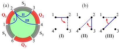
Figure 2: Braiding process. (a) An FTI disk with six SC/FM segments. In stages I, II and III of the braiding process, quasi-particle tunneling (represented by blue solid lines) is turned on between the SC/FM interfaces. (b) Representation of the braiding procedure, involving interfaces 1, 2, 3 and 4. In the beginning of each stage, the two interfaces connected by a solid line are coupled; during that stage, the bond represented by a dashed line is adiabatically turned on, and simultaneously the solid bond is turned off. By the end of stage III, the system returns to the original configuration.

The braiding process is facilitated by deforming the droplet adiabatically, such that different SC/FM interfaces are brought close to each other at every stage. Proximity between interfaces essentially couples them, by allowing quasi-particles to tunnel between them. We shall assume that only one spin species can tunnel between interfaces. The reason for this assumption will become clear in next sections, and we shall explain how it is manifested in realizations of the model under consideration. At the end of the process, the droplet returns to its original form, but the state of the system does not return to the initial state. The adiabatic evolution corresponds to a unitary matrix acting on the ground state manifold.

Below, we analyze a braid operation between nearest-neighbor interfaces, which we label $3$ and $4$ (for later convenience). The operation consists of three stages, which are described pictorially in Fig. 2b. It begins by nucleating a new, small, segment which is flanked by the interfaces $1$ and $2$. At the beginning of the first stage, the small size of the new segment means that interfaces $1$ and $2$ are coupled to each other, and all the other interfaces are decoupled. During the first stage, we simultaneously bring interface $3$ close to $2$, while moving $1$ away from both $2$ and $3$, such that at the end of the process only $2$ and $3$ are coupled to each other, while $1$ is decoupled from them. In the second stage, interface $4$ approaches $3$, and $2$ is taken away from $3$ and $4$. In the final stage, we couple $1$ to $2$ and decouple $4$ from $1$ and $2$, such that the Hamiltonian returns to its initial form. In the following, we analyze an explicit Hamiltonian path yielding this braid operation, which is summarized in Table 1. Later, we shall discuss the conditions under which the result is independent of the specific from of the Hamiltonian path representing the same Braid operation.

Table 1: Summary of the braiding adiabatic trajectory (shown also in Fig. 2b). There are three stages, $\alpha=\mathrm{I,II,III}$, along each of which the parameter $\lambda_{\alpha}$ varies from $0$ to $1$. The Hamlitonian in each stage is written in the middle column, where we use the notation $H_{ij}=-t_{ij}\chi_{j,\uparrow}\chi_{i,\uparrow}^{\dagger}+h.c.$ ($t_{ij}$ are complex parameters). The right column summarizes the symmetry operators which commute with the Hamiltonian throughout each stage.

Stage	Hamiltonian	Symmetries
I	$\left(1-\lambda_{\mathrm{I}}\right)H_{12}$+$\lambda_{\mathrm{I}}H_{23}$	$e^{i\pi\hat{Q}_{3}}$, $e^{i\pi\hat{S}_{3}}$
II	$\left(1-\lambda_{\mathrm{II}}\right)H_{23}$+$\lambda_{\mathrm{II}}H_{24}$	$e^{i\pi\hat{Q}_{3}}$, $e^{-i\pi\hat{S}_{1}}$
III	$\left(1-\lambda_{\mathrm{III}}\right)H_{24}$+$\lambda_{\mathrm{III}}H_{12}$	$e^{i\pi\hat{Q}_{3}}$, $e^{-i\pi\hat{Q}_{2}}e^{i\pi\hat{S}_{3}}$

VI.2 Ground state degeneracy

To analyze the braiding process, we first need to show that it does not change the ground state degeneracy. We consider a disk with a total of $N=3$ segments of each type. The ground state manifold, without any coupling, is $(2m)^{2}$ fold degenerate. We define operators $H_{12},H_{23}$ and $H_{24}$, the Hamiltonians at the beginning of the three stages I, II, III. These are given by

$$H_{jk}=-t_{jk}\chi_{j,\uparrow}^{\vphantom{\dagger}}\chi_{k,\uparrow}^{\dagger}+h.c..$$ (13)

where the $t_{jk}$ are complex amplitudes.

Consider first the initial Hamiltonian (see Table 1), given by

$$H_{12}=-t_{12}\chi_{2,\uparrow}^{\vphantom{\dagger}}\chi_{1,\uparrow}^{\dagger}+h.c.=-2\left|t_{12}\right|\cos\left(\pi\hat{Q}_{1}+\varphi_{12}\right).$$ (14)

Here, $\varphi_{12}=\arg\left(t_{12}\right)$. It is convenient to work in the basis of eigenstates of the operators $e^{i\pi\hat{Q}_{1}}$, $e^{i\pi\hat{Q}_{2}}$, $e^{i\pi\hat{Q}_{3}}$, and $e^{i\pi\hat{S}_{\mathrm{tot}}}$, which we label by $|q_{1},q_{2},q_{3};s\rangle$. The total charge and spin are conserved, and we may set $\sum_{j}q_{j}=0$ and $s=0$. Then, a state in the $\left(2m\right)^{2}$-dimensional low-energy subspace can be labelled as $|q_{2},q_{3}\rangle$, where $q_{1}$ is fixed to $q_{1}=-q_{2}-q_{3}$. The initial Hamiltonian (14) is diagonal in this basis, and therefore its eigen-energies can be read off easily: $E_{12}\left(q_{2},q_{3}\right)=-2\left|t_{12}\right|\cos\left[-\frac{\pi}{m}\left(q_{2}+q_{3}\right)+\varphi_{12}\right]$. For generic $\varphi_{12},$ there are $2m$ ground states. Since this FM segment is nucleated inside a SC region, its total spin is zero, and the ground states are

$$|\Psi_{i}(q_{3})\rangle=|q_{2}=-q_{3},q_{3}\rangle,$$ (15)

labelled by a single index $q_{3}=0,\dots,2m-1$. The residual $2m$-fold ground state degeneracy can be understood as a result of the symmetries of the Hamiltonian. From Eq. (14) $e^{i\pi\hat{Q}_{3}}$ and ${e^{i\pi\hat{S}_{3}}}$ commute with $H_{12}$. The commutation relations between $e^{i\pi\hat{Q}_{3}}$ and ${e^{i\pi\hat{S}_{3}}}$ ensures that the ground state is (at least) $2m$-fold degenerate by the eignevalues of $e^{i\pi\hat{Q}_{3}}$.

Similar considerations can be applied in order to find the ground state degeneracy throughout the braiding operation. The operator $e^{i\pi\hat{Q}_{3}}$ always commutes with the Hamiltonian, at any stage. This can be seen easily from the fact that the segment labelled by $e^{i\pi\hat{Q}_{3}}$ never couples to any other segment at any stage (see Fig. 2a). Using the definition of the $\chi_{i\sigma}$ operators, Eq. (11), one finds that

$$H_{23}=-2\left|t_{23}\right|\cos\left(\pi\hat{S}_{2}+\varphi_{23}\right),$$ (16)

and

$$H_{24}=-2\left|t_{24}\right|\cos\left[\pi\left(\hat{S}_{2}+\hat{Q}_{2}\right)+\varphi_{24}\right].$$ (17)

In each stage, $\alpha=\mathrm{I,II,III}$, there is a symmetry operator $\Sigma_{\alpha}$ that commutes with the Hamiltonian, and satisfies $\Sigma_{\alpha}e^{i\pi\hat{Q}_{3}}=e^{-i\frac{\pi}{m}}e^{i\pi\hat{Q}_{3}}\Sigma_{\alpha}$. We specify $\Sigma_{\alpha}$ for each stage in the right column of Table 1, and the aforementioned relation can be verified using Eq. (2). This combination of symmetries dictates that every state is at least $2m$ fold degenerate, where each degenerate subspace can be labelled by $q_{3}$. Assuming that the special values $\varphi_{12},\varphi_{23}=\pi(2l+1)/(2m)$ and $\varphi_{24}=\pi l/m$ ($l$ integer) are avoided, the ground state is exactly $2m$-fold degenerate throughout the braiding process (the special values for the $\varphi_{ij}$ give an additional two fold degeneracy). Note that these conclusions hold for any trajectory in Hamiltonian space, as long as the appropriate symmetries are maintained in each stage of the evolution, and the accidental degeneracies are avoided.

VI.3 Braid matrices from Berry’s phases

The evolution operator corresponding to the braid operation can thus be represented as a block-diagonal unitary matrix, in which each $\left(2m\right)\times\left(2m\right)$ block acts on a separate energy subspace. We are now faced with the problem of calculating the evolution operator in the ground state subspace. Let us denote this operator by $\hat{U}_{34}$, corresponding to a braiding operation of interfaces 3 and 4. The calculation of $\hat{U}_{34}$ can be done analytically by using the symmetry properties of Hamiltonian at each stage of the evolution.

We begin by observing that, since $e^{i\pi\hat{Q}_{3}}$ always commutes with the Hamiltonian, $\hat{U}_{34}$ and the evolution operators for each stage are diagonal in the the basis of $e^{i\pi\hat{Q}_{3}}$ eigenstates. In every stage, the adiabatic evolution maps $e^{i\pi\hat{Q}_{3}}$ eigenstates between the initial and final ground state manifolds while preserving the eigenvalue $q_{3}$, and multiplies by a phase factor that may depend on $q_{3}$. This is explicitly summarized as

$$\hat{U}_{\alpha}|\Psi^{\alpha}_{i}(q_{3})\rangle=\exp{\big{(}i\gamma_{\alpha}\left(q_{3}\right)\big{)}}|\Psi^{\alpha}_{f}(q_{3})\rangle.$$ (18)

Here, $\hat{U}_{\alpha}$ is the evolution operator of stage $\alpha=\mathrm{I,II,III}$, and $|\Psi^{\alpha}_{i(f)}(q_{3})\rangle$ are the ground states of the initial (final) Hamiltonian in stage $\alpha$, respectively, which are labelled by their $e^{i\pi\hat{Q}_{3}}$ eigenvalues. Likewise, $\gamma_{\alpha}\left(q_{3}\right)$ are the phases accumulated in each of the stages.

In order to determine $\gamma_{\alpha}\left(q_{3}\right)$, we use the additional symmetry operator $\Sigma_{\alpha}$ for each stage, as indicated in Table 1. This symmetry commutes with the Hamiltonian, and therefore also with the evolution operator for this stage $[\Sigma_{\alpha},\hat{U}_{\alpha}]=0$. Acting with $\Sigma_{\alpha}$ on both sides of (18), we get that

$$\hat{U}_{\alpha}\Sigma_{\alpha}|\Psi^{\alpha}_{i}(q_{3})\rangle=e^{i\gamma_{\alpha}\left(q_{3}\right)}\Sigma_{\alpha}|\Psi^{\alpha}_{f}(q_{3})\rangle.$$ (19)

Furthermore, the relation $e^{i\pi\hat{Q}_{3}}\Sigma_{\alpha}=e^{i\frac{\pi}{m}}\Sigma_{\alpha}e^{i\pi\hat{Q}_{3}}$ implies that the operator $\Sigma_{\alpha}$ advances $e^{i\pi\hat{Q}_{3}}$ by one increment, and therefore for both the initial and final stage at each stage we have,

$$\Sigma_{\alpha}|\Psi^{\alpha}_{i(f)}(q_{3})\rangle =\exp{\left(i\delta^{\alpha}_{i(f)}\left(q_{3}\right)\right)}|\Psi^{\alpha}_{i(f)}(q_{3}+1)\rangle,$$ (20)

where $\delta^{\alpha}_{i(f)}\left(q_{3}\right)$ are phases which depends on gauge choices for the different eigenstates, to be determined below. Inserting (20) into (19), we get the recursion relation

$$\gamma_{\alpha}\left(q_{3}+1\right)=\gamma_{\mathrm{\alpha}}\left(q_{3}\right)+\delta^{\alpha}_{f}\left(q_{3}\right)-\delta^{\alpha}_{i}\left(q_{3}\right).$$ (21)

Note that while the phase accumulation at each point along the path depends on gauge choices, the total Berry phase accumulated along a cycle does not. It is convenient to choose a continuous gauge, for which the total Berry’s phases are given by

$$\hat{U}_{34}|\Psi^{\alpha}_{i}(q_{3})\rangle=\exp{\big{(}i\sum_{\alpha}\gamma_{\alpha}\left(q_{3}\right)\big{)}}|\Psi^{\alpha}_{i}(q_{3})\rangle.$$ (22)

A continuous gauge requires $|\Psi_{f}^{\alpha}(n_{3})\rangle=|\Psi_{i}^{\alpha+1}(n_{3})\rangle$. Therefore, the values of the phases $\delta^{\alpha}_{i(f)}$ depend only on three gauge choices. These are the gauge choices eigenstates of the Hamiltonians $H_{12}$, $H_{23}$, and $H_{24}$, which constitute the initial Hamiltonian at the beginning of stages I-III, as well as the final Hamiltonian for stage III.

Making the necessary gauge choice, allows us to solve Eq. (21) for $\gamma_{\alpha}(n_{3})$, yielding the total Berry phase (the details of the calculation are given in Appendix B)

$$\gamma\left(q_{3}\right)=\frac{\pi}{2m}(q_{3}-k)^{2}.$$ (23)

The integer $k$ depends on the choice for the phases $\varphi_{ij}$. Recall that the Hamiltonians $H_{ij}$, Eqs. (14),(16–17), have an additional degeneracy for a discrete choice of the $\varphi_{ij}$. Any two choices for the $\varphi_{ij}$ that can be deformed to each other without crossing a degeneracy point yield the same $k$.

The evolution operator for the braiding path can be written explicitly by its application on the eigenstates of the Hamiltonian in the beginning of the cycle, $\hat{U}^{(k)}_{34}|\Psi_{i}(q_{3})\rangle=e^{i\frac{\pi}{2m}(q_{3}-k)^{2}}|\Psi_{i}(q_{3})\rangle$. Since by Eq. (15), the ground states of the initial Hamiltonian satisfy $q_{2}=-q_{3}$, this can be written in a basis-independent form in terms of the operator $e^{i\pi\hat{Q}_{2}}$. Loosely speaking, $\hat{U}_{34}$ can be written as

$$\hat{U}^{(k)}_{34}=\exp\left(\frac{i\pi m}{2}\left(\hat{Q}_{2}-\frac{k}{m}\right)^{2}\right).$$ (24)

Alternatively, using the identitygau $e^{i\frac{\pi}{2m}q^{2}}=\sqrt{\frac{1}{2m}}\sum_{p=0}^{2m-1}e^{i\frac{\pi}{m}\left(pq-\frac{p^{2}}{2}\right)+i\frac{\pi}{4}}$, one can write

$$\hat{U}^{(k)}_{34}=\sqrt{\frac{1}{2m}}\sum_{p=0}^{2m-1}e^{-\frac{i\pi}{2m}(p+k)^{2}+i\frac{\pi}{4}}\left(e^{i\pi\hat{Q}_{2}}\right)^{p}.$$ (25)

In the case $m=1$, $\hat{U}_{34}$ reduces to the braiding rule of Ising anyons Ivanov (2001); Read and Green (2000); Nayak and Wilczek (1996).

Following a similar procedure, one can construct the operator representing the exchange of any pair of neighboring interfaces: $\hat{U}^{(k)}_{2j-1,2j}=e^{\frac{i\pi m}{2}\left(\hat{S}_{j}-k/m\right)^{2}}$, $\hat{U}^{(k)}_{2j,2j+1}=e^{\frac{i\pi m}{2}\left(\hat{Q}_{j+1}-k/m\right)^{2}}$. In order for these operations to form a representation of the braid group, it is necessary and sufficient that they satisfy

$$\left[\hat{U}^{(k_{i})}_{i,i+1},\hat{U}^{(k_{j})}_{j,j+1}\right] =0\,\,\,(\left|i-j\right|>1),$$ (26)

$$\hat{U}^{(k_{1})}_{j,j+1}\hat{U}^{(k_{2})}_{j+1,j+2}\hat{U}^{(k_{1})}_{j,j+1} =\hat{U}^{(k_{2})}_{j+1,j+2}\hat{U}^{(k_{1})}_{j,j+1}\hat{U}^{(k_{2})}_{j+1,j+2}.$$ (27)

Equation (26) clearly holds because the spin or charge operators of non-nearest neighbor segments commute. Using (25), it is not difficult to show that (27) holds as well (see Appendix D. Eq. (27) is depicted in Fig. 3). Therefore, $\hat{U}_{i,i+1}$ form a representation of the braid group. In that respect, our system exhibits a form of non-abelian statistics. By combining a sequence of nearest-neighbor exchanges, an exchange operation of arbitrarily far segments can be defined.

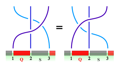
Figure 3: Diagrammatic representation of the Yang-Baxter equations (Eq. 75). Three interfaces 1,2,3 are braided in two distinct sequences. The Yang-Baxter equations state that the results of these two sequences of braiding operations are the same.

In any physical realization, we do not expect to control the precise form of the Hamiltonian in each stage. It is therefore important to discuss the extent to which the result of the braiding process depends on the details of the Hamiltonian along the path. We argue that the braiding is “topological”, in the sense that it is, to a large degree, independent of these precise details.

To see this, one needs to note that the braiding unitary matrix was derived above without referring to the precise adiabatic path in Hamiltonian space. All we used were the symmetry properties of the Hamiltonian in each stage (Table 1). These symmetries do not depend on the precise details of the intermediate Hamiltonian, but only on the overall configuration, e.g., which interfaces are allowed to couple in each stage.

In Appendix C.1, we state more formally the conditions under which the result of the braiding is independent of details. Special care must be taken in stage III of the braiding, in which quasi-particles of only one spin species, e.g. spin up, must be allowed to tunnel between interfaces 2 and 4. We elaborate on the significance of this requirement and the ways to meet it in the various physical realizations in Appendix C.2.

VII Braiding and topological spin of boundary anyons

In the previous section, we derived the unitary matrix representing braid operations by an explicit calculation. In the following, we shall try to shed light on the physical picture behind these representations. To do so, we show that the results of the previous section can be derived almost painlessly, just by assuming that the representation of the braids have properties which are analogous to those of anyons in two dimensions. The first and most basic assumption, is very natural: there exists a topological operation in the system which corresponds to a braid of two interfaces, in that the unitary matrices representing this operation obey the Yang-Baxter equation.

The operations we consider braid two neighboring interfaces, but do not change the total charge (spin) in the segment between them. This results from the general form of the braid operations - to exchange two interfaces flanking a SC (FM) segment, we use couplings to an auxiliary segment, of the same type. Therefore, charge (spin) can only be exchanged with the auxiliary segment. Since the auxiliary segment has zero charge (spin) at the beginning and end of the operation, the charge of the main segment cannot change by the operation. Indeed, this can be seen explicitly in the analysis presented in the previous section. As a result, the unitary matrix representing the braid operation is diagonal with respect to the charge (spin) of the segment.

The derivation now proceeds by considering a property of anyons called the topological spin (TS). In two dimensions, the topological spin gives the phase acquired by a $2\pi$ rotation of an anyon. For fermions and bosons, the topological spin is the familiar $-1$ and $+1$ respectively (corresponding to half-odd or integer spins). There is a close connection between the braid matrix for anyons and their topological spin. In two dimensions, these relations have been considered by various authors Kitaev (2006); Preskill (2004). The system under consideration is one dimensional, and therefore seemingly does not allow a $2\pi$ “rotation” of a particle. However, as we shall explain below, the TS of a particle can be defined in our system using the relations of the TS to the braid matrix. We shall then see how to use these relations to derive the possible unitary representations of the braid operations in the system at point.

In our one dimensional system, we consider the TS of two different kinds of objects (particles) - interfaces, which we denote by $X$, and the charge (or spin) of a segment, which we shall label by $q=0,1,..2m-1$. In what follows, we need to know how to compose, or fuse different objects in our system. As we saw above, two interfaces yield a quantum number $\exp(i\pi Q)$ ($\exp(i\pi S)$) which is the total charge (spin) in the segment between them, respectively. Suppose we consider two neighboring SC segments with quantum numbers $\exp(i\pi Q_{1})$ and $\exp(i\pi Q_{2})$, and we “fuse” them by shrinking the FM region which lies between them. This results in tunneling of fractional quasi-particles between the two SC regions, and energetically favors a specific value for $\exp(i\pi S)$ in the FM region. The two SC segments are for all purposes one, where clearly, in the absence of other couplings, $\exp\left(i\pi(Q_{1}+Q_{2})\right)$ remains a good quantum number. This therefore suggests the following fusion rules

$$X\times X = 0+1+...+2m-1$$

$$q_{1}\times q_{2} = (q_{1}+q_{2})\mod 2m$$ (28)

We note that the labelling $q_{1}=0,1...,2m-1$ does not depend on the gauge choices in the definition of the operators $\exp(i\ \pi Q)$. Equation (28) suggests that the labelling can be defined by the addition law for charges, in which each type of charge plays a different role. Indeed, this addition rule has a measurable physical content which does not depend on any gauge choices.

In two dimensional theories of anyons, it is convenient to think about particles moving in the two dimensional plane, and consider topological properties of their world lines (such as braiding). In this paper, we have defined braiding by considering trajectories in Hamiltonian space. In the following, we represent these Hamiltonian trajectories as world-lines of the respective “particles” involved, keeping in mind that they do not correspond to motion of objects in real space.

We are now ready to define the TS in our system. In short, the TS of a particle is a phase factor associated to the world line appearing in Fig 4(a). For interfaces, it is concretely defined by the phase acquired by the system by the following sequence of operations, as illustrated in Fig 4(e): (i) nucleation of a segment to the right (by convention) of the interface $X_{1}$ (note that the notation $X_{1}$ corresponds to particle $X$ at coordinate $r_{1}$). The total spin or charge of this segment is zero (the nucleation does not add total charge to the system). The couplings between $X_{2}$ and $X_{3}$ flanking the new segment is taken to zero, increasing the ground state degeneracy by a factor of $2m$. (ii) A right handed braid operation is performed between $X_{1}$ and $X_{2}$. (iii) The total charge $q$ of the segment between $X_{2}$ and $X_{3}$ is measured, and we consider (post-select) only the outcomes corresponding to zero charge. Therefore, the system ends up in the same state (no charges have been changed anywhere in the system), up to a phase factor. Importantly, this phase factor does not depend on the state of the system, since the operation does not change the total charge in the segment of $X_{1}$ and $X_{2}$ (see Appendix E for a more detailed discussion). We can therefore define this phase factor as $\theta_{X}$, the topological spin of particle type $X$.

In order to define $\theta_{q}$, the topological spin of a charge $q$, we first need to define the operation corresponding to an exchange of two charges. Consider the sequence of $4$ right handed exchanges of the interfaces, as in Fig. 4 (c). The figure suggests that this sequence should yield an exchange of the fusion charges $q_{1}$ and $q_{2}$ of the two pairs of $X$ particles, as would indeed be the case for anyons in two dimensions (see Appendix. E for more details). Our second assumption is that this is indeed the case. Since by Eq. (28) there is only one fusion channel for the $q_{i}$’s, the state is multiplied by a phase factor which depends only on $q_{1}$ and $q_{2}$ - the charges $q_{i}$ are abelian. It is straightforward to check that exchanges of charges satisfy the Yang-Baxter equation.

The operations defining $\theta_{q}$ are illustrated in Figs 4(b) and (f). We consider, say, a SC segment in an eigenstate of $\exp(i\pi Q_{1})$ to which we associate a particle type $q_{1}$. In step (i), we nucleate two segments to the right of $q_{1}$. This step is actually done in two substeps: first, we nucleate a SC segment to the right of the segment $q_{1}$, and then we nucleate a FM segment which separates this segment into two segments, with charges $\exp\left(i\pi\left(Q_{2}+Q_{3}\right)\right)=1$. Note that the spin of the middle FM segment is also zero, $\exp\left(i\pi S_{2}\right)=1$. We now perform a braid between the segments labelled $q_{1}$ and $q_{2}$. Next, we measure the charges $\exp\left(i\pi\left(Q_{2}+Q_{3}\right)\right)$ and $\exp(i\pi S)$, post-selecting their values to be equal to $1$. The charge $q_{1}$ in the original segment is therefore unchanged by this sequence of operations, as well as any other charges used to label the original state of the system. As before, the state of the system acquires a phase, which only depends on the charge $q_{1}$.

We now use an important relation between the TS of a composite to a double braid of its two components. This is a result of an equality between Fig 4 (b) and (d), which can be derived by using the Yang-Baxter equation and the definition for the TS. The equality between Fig. 4 (b) and (d), with both incoming and outgoing lines labelled by $X$, yields

$$\theta_{q}=\theta_{X}^{2}U^{2}(q)$$ (29)

where $U(q)$ corresponds to the unitary matrix representing an exchange of two interfaces whose fusion charge is $q$. We shall not attempt to calculate $\theta_{X}$. However, by calculating the topological spin $\theta_{q}$ of the composite, we can get, using Eq. (29), the square of the sought after braid matrix, up to a global phase.

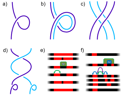
Figure 4: Topological Spin. The process illustrated in (a) defines the TS, where the cup $\bigcup$ corresponds to creation of a particle -anti particle pair (two $X$’s fusing to $q=0$ or two charges with $q_{1}+q_{2}=0$), and the cap $\bigcap$ corresponds to projection on zero total charge. (b) TS of a composite object. When both lines are labelled by $X$ and fuse to charge $q$ , the phase acquired is $\theta_{q}$. The $4$-fold crossing, which is magnified in (c), is assumed to result in an exchange of two $q$’s. When the lines are labelled by $q_{1}$ and $q_{2}$, the phase acquired is $\theta_{q_{1}+q_{2}\mod 2m}$. Importantly, the TS of a composite is equal to the phase accumulated in the process appearing in (d). This equality results from using the Yang-Baxter equation and the definition of the TS. (e) The evolution of the different segments in the process defining $\theta_{X}$. The green arrow corresponds to braiding, while the “M” corresponds to projection on zero charge. (f) The process defining $\theta_{q}$. The braids are ordered by color, green, blue and finally purple. The projections are on zero spin for the magnet segment intersecting the two SC segments, and zero total charge for these two segments.

In two dimensional theories of anyons, the TS of a composite of two particles is equal to the TS of the particle they fuse into. This can be understood by noting that the equality between Fig 4 (b) and (d) guarantees that in two dimensions, the TS of the composite includes both the intrinsic spin of the two particles and their relative angular momentum (see Appendix E for more details). We now assume the same holds in our one dimensional system - the TS of the $q_{1}$, $q_{2}$ composite is equal to the TS of combined $q=q_{1}+q_{2}\mod 2m$ charge. The TS of a composite of two charges $q_{1}$ and $q_{2}$ is just the process described in Fig. 4(b), with the outgoing lines are labelled with $q_{1}$ and $q_{2}$.

Next, we note that for consistency, the charge $q=0$ must correspond to trivial TS, $\theta_{0}=1$. We take the TS of the elementary charge $q=1$ as a parameter, $\theta_{1}=e^{i\alpha}$, to be determined later. Importantly, note that Fig. 4(a) implies that an exchange of two segments with $q=1$ leads to the phase factor $\theta_{1}$. Using the composition rule in Eq. (28), $\theta_{q}$ should be equal to the TS of a composite of $q$ unit charges, a process where we encounter $q^{2}$ exchanges of these elementary charges. This gives for the topological spin

$$\theta_{q\!\!\!\mod 2m}=\exp{\left(i\alpha q^{2}\right)}.$$ (30)

The $\mathbb{Z}_{2m}$ structure above appears since fusing $2m$ elementary particles results in the trivial $q=0$ charge, and requires that

$$\alpha=\frac{\pi p}{2m},\qquad p\in\mathbb{Z}.$$ (31)

Taking the square root of Eq. (30) we arrive at

$$U(q)=(-1)^{f(q)}\exp{\left(i\frac{\alpha}{2}q^{2}\right)}.$$ (32)

where $f(q)$ is an arbitrary, integer valued function. To determine $\alpha$ and $f(q)$ we appeal to the Yang-Baxter equation, Eq. (27). We find numerically that solutions are possible only for even $p$’s in Eq. (31), where sign function $(-1)^{f(q)}$ can be of the form $e^{i\pi(n_{1}q^{2}+n_{2})}$ with integer $n_{1},n_{2}$. Therefore, the extra $(-1)$ signs can always be absorbed in the definition of $\alpha$, up to an overall sign. The final result is therefore

$$U(q)=\exp{\left(i\frac{\pi n}{2m}q^{2}\right)},\qquad n\in\mathbb{Z}.$$ (33)

As noted in Sec. II, the value $n=1$ is realized by quasi-particle tunnelling of a single spin species, while $n=m$ is realized by electron tunnelling. The other representations of the braid group, which are given by $U^{(k)}(q)=\exp{\left(i\frac{\pi n}{2m}(q-k)^{2}\right)}$ can be obtained from the above considerations by adding more particles types. Indeed, we see that

$$U^{(k)}(q)\left(U^{(k-1)}(q)\right)^{{\dagger}}=e^{-i\frac{\pi n}{2m}(2k-1)}e^{i\frac{\pi n}{m}q}$$ (34)

is, up to a global phase, a topological operation which is equivalent to taking a vortex $n$ times around a SC segment, or changing the orientation of the FM direction $n$ times in the $x-y$ plane by $2\pi$.

VIII Quantum information processing

In order to assess the suitability of our system for topologically protected quantum computation, it is instructive to examine the structure of the resulting non-abelian theory. Below, we show that the representation of the braid group realized in our system is a direct product of an Ising anyonic theory times a novel representation of dimension $m$. We argue that braiding operations alone are not sufficient to realize universal topologically protected quantum computation, in agreement with the general argument for models with anyons of quantum dimension which is a square root of an integerRowell et al. (2009).

The unitary matrix that describes the braiding operation of two interfaces at the ends of a superconducting segment, Eq. (24), depends on the charge in the superconducting segment. The charge can be written as $Q=q/m$ where $q$ can be uniquely expressed as $q=mq_{\sigma}+2q_{\upsilon}$, with $q_{\sigma}=0,1$ and $q_{\upsilon}=0,\dots,m-1$. Inserting this expression into Eq. (24), and assuming for simplicity $k=0$, we get

$$\hat{U}=e^{\frac{i\pi}{2}q_{\sigma}^{2}}e^{\frac{2i\pi}{m}q_{\upsilon}^{2}}.$$ (35)

Therefore, we see that if we write the Hilbert space $\mathcal{H}$ as a tensor product $\mathcal{H_{\sigma}}\otimes\mathcal{H_{\upsilon}}$, such that the states are written as $|q\rangle=|q_{\sigma}\rangle\otimes|q_{\upsilon}\rangle$, the braiding matrix decomposes into a tensor product $\hat{U}_{\sigma}\otimes\hat{U}_{\upsilon}$. Here, $\hat{U}_{\sigma}$ and $\hat{U}_{\upsilon}$ are $2\times 2$ and $m\times m$ matrices, given by the first and second terms on the right hand side of Eq. (35), respectively. A similar decomposition holds for a braid operation acting on a ferromagnetic segment. In this respect, we see that the $2m$-dimensional representation of the braid group given by Eq. (24) is reducible: it decomposes into a two-dimensional representation, which is nothing but the representation formed by Ising anyons $\sigma$, times an $m$-dimensional representation corresponding to braiding of a non-Ising object $\upsilon$.

This decomposition gives insights into the class of unitary transformations that can be realized using braiding of interfaces, and hence their suitability for quantum computation. We now argue that by using braiding operations alone, the system studied in this paper does not allow for topologically protected universal quantum computation. Ising anyons are known not to provide universality for quantum computation Nayak et al. (2008); Freedman et al. (2006, 2002). Due to the tensor product structure of the topologically protected operations, it is sufficient to consider the fractional part, corresponding to $\mathcal{H_{\upsilon}}$. The braid representations acting within this subspace preservesus- a generalization of the Pauli group to q-dits of dimension $m$. Therefore, the braid operations can be simulated on a classical computer, and are not universal.

Conceptually, universality could be achieved by adding an entangling operation between the Ising and the fractional parts. A braiding operation would then produce an effective phase gate that would provide the missing ingredient to make the Ising part universal. However, at present we do not know whether it is possible to realize such an operation in a topologically protected way. Moreover, topologically protected measurements of charges Hassler et al. (2010) (and spins) cannot achieve such entanglement, since similarly to the braiding, they can also be shown to be of a tensor product form.

IX Concluding remarks

In this work, we have described a physical route for utilizing proximity coupling to superconductors in order to realize a species of non-abelian anyons, which goes beyond the Majorana fermion paradigm. The essential ingredients of the proposed system are a pair of counter-propagating edge modes of a Laughlin fractional quantum Hall state, proximity-coupled to a superconductor. As we saw, there are several possible realizations of such a system. One could start from a “fractional topological insulator” whose edges are coupled to an array of superconductors and ferromagnets. In the absence of any known realization of a fractional topological insulator phase (as of today), one could get by starting from “ordinary” Laughlin fractional quantum Hall state whose edges are coupled to a superconductor. The fractional quantum Hall state in graphene might be a promising candidate for realizing such systems, since the magnetic fields needed for observing it are much lower than the fields needed in semiconductor heterostructure devices.

An experimentally accessible signature of the fractionalized Majorana modes is a fractional Josephson effect, which should exhibit a component of $4m\pi$ periodicity (analogously to the $4\pi$ periodicity predicted for topological superconductors with Majorana edge modesFu and Kane (2009); Jiang et al. (2011)). In addition, it might be possible to observe topological pumping of fractional charge by controlling the relative phase of the superconducting regions.

More broadly speaking, the system we describe here is an example of how gapping out the edge state of a fractionalized two-dimensional phase can realize a topological phase which supports new types of non-abelian particles, not present in the original two-dimensional theory. In our example, the underlying Laughlin fractional quantum Hall state supports quasiparticles with a fractional charge and fractionalized abelian statistics; the resulting gapped theory on the edge, however, realizes non-abelian quasiparticles. Moreover, the resulting non-abelian theory on the edge is shown to go beyond the well-known Majorana (Ising) framework.

This may seem contradictory to the general argumentsFidkowski and Kitaev (2010, 2011); Turner et al. (2011); Chen et al. (2011); Schuch et al. (2011) indicating that gapped one-dimensional systems with no symmetry other than fermion parity conservation support only two distinct topological phases, a trivial phase and a non-trivial phase, with an odd number of Majorana modes at the interface between them. The reason our system avoids this exhaustive classification is that it is not, strictly speaking, one-dimensional; the edge states of fractional quantum Hall states can never be realized as degrees of freedom of an isolated one-dimensional system. This is reflected, for example, in the fact that the theory contains “local” (from the edge perspective) operators which satisfy fractional statistics, which is not possible in any one-dimensional system made of fermions and bosons.

It would be interesting to pursue this idea further, by examining gapped states which are realized by gapping out edge modes of topological phases. This may serve as a route to discovering new classes of topological phases with non-abelian excitations. For example, more complicated Halperin (1984) quantum Hall states or higher dimensional fractional topological insulatorsLevin et al. (2011); Swingle et al. (2011); Maciejko et al. (2010) may be interesting candidates for such investigations.

Note added.- During the course of working on this manuscript, we became aware that a similar idea is being pursued by David Clarke, Jason Alicea, and Kirill ShtengelClarke et al. . After this manuscript was submitted, two papers on related subjectsCheng ; Vaezi have appeared.

Appendix A Appendix: Matrix elements of the quasi-particle operator

In this Appendix, we describe an explicit calculation of the matrix element of a quasi-particle operator between different states in the ground state manifold. We show that the matrix element is finite if the quasi-particle is located sufficiently close to an interface between a superconducting and a ferromagnetic segment. The matrix element decays exponentially with the distance from the interface.

A.1 Model

Let us consider a system composed of one superconducting segment, extending from $x=0$ to $x=L$, between two long ferromagnetic segments at $x<0$ and $x>L$. For simplicity, we assume that the gap in the ferromagnetic segments is very large, such that charge fluctuations are completely quenched outside the superconductor. The Hamiltonian for $0\leq x\leq L$ is

$$H =\int_{0}^{L}dx\left\{\frac{m}{2\pi}u\left[\left(\partial_{x}\phi\right)^{2}+\left(\partial_{x}\theta\right)^{2}\right]-g_{S}\cos\left(2m\phi\right)\right\}$$

supplemented by the boundary condition

$$\partial_{x}\phi\left(x=0,L\right)=0,$$ (37)

which accounts for the fact that the current at the edges of the superconductor is identically zero, due to the large gap in the ferromagnetic regions. We are assuming that the coupling $g_{S}$ is large enough such that the field $\phi$ is pinned to the vicinity of the minima of the cosine potential, $\phi\approx\frac{\pi}{m}l$, where $l$ is an integer. Deep in the superconducting phase, one can expand the cosine potential up to second order around one of the minima, obtaining the effective Hamiltonian

$$H_{\mathrm{eff}} =\int_{0}^{L}dx\left\{\frac{m}{2\pi}u\left[\left(\partial_{x}\phi\right)^{2}+\left(\partial_{x}\theta\right)^{2}\right]+\frac{g}{2}\left(\phi-\frac{\pi l}{m}\right)^{2}\right\},$$

where $g\equiv\left(2m\right)^{2}g_{S}$.

The Hamiltonian (LABEL:eq:Hquad) is quadratic, and can be diagonalized using the following mode expansion:

$$\phi\left(x\right)=\frac{\pi}{m}l+\hat{\phi}_{0}+i\frac{1}{\sqrt{m}}\sum_{k=1}^{\infty}\sqrt{\frac{1}{k}}\cos\left[\frac{\pi k}{L}x\right]\left(a_{k}-a_{k}^{\dagger}\right),$$ (39)

$$\theta\left(x\right)=\theta\left(0\right)+\frac{\pi\hat{n}}{mL}x+\frac{1}{\sqrt{m}}\sum_{k=1}^{\infty}\sqrt{\frac{1}{k}}\sin\left[\frac{\pi k}{L}x\right]\left(a_{k}+a_{k}^{\dagger}\right).$$ (40)

Here, we have introduced the ladder operators $a_{k}$, $k=1,2,\dots,$ satisfying $\left[a_{k},a_{k^{\prime}}^{\dagger}\right]=\delta_{k,k^{\prime}}$ and $\left[a_{k},a_{k^{\prime}}\right]=0$. $\hat{\phi}_{0}$ and $\hat{n}$ are the average phase and the charge of the superconducting segment. These variables are canonical conjugates, satisfying $\left[\hat{\phi}_{0},\hat{n}\right]=i$. Note that $\left[\theta\left(0\right),H_{\mathrm{eff}}\right]=0$, therefore $\theta\left(0\right)$ can be replaced by a c-number:

$$\theta\left(0\right)=\frac{\pi}{m}p,$$ (41)

with integer $p$, where we have assumed that these values minimize the (infinite) cosine potential on the ferromagnetic side $x<0$. Using Eq. (39),(40), one can reproduce the commutation relation $\left[\phi\left(x\right),\theta\left(x^{\prime}\right)\right]=i\frac{\pi}{m}\Theta\left(x^{\prime}-x\right)$.

Inserting the mode expansions into the Hamiltonian (LABEL:eq:Hquad), we get

$$H_{\mathrm{\mathrm{eff}}} =\frac{\pi u}{2mL}\hat{n}^{2}+\frac{gL}{2}\hat{\phi}_{0}^{2}+\sum_{k=1}^{\infty}\left(\frac{\pi uk}{2L}+\frac{gL}{4mk}\right)\left[a_{k}^{\dagger}a_{k}+a_{k}a_{k}^{\dagger}\right]$$

$$-\sum_{k=1}^{\infty}\frac{gL}{4mk}\left(a_{k}^{2}+a_{k}^{\dagger 2}\right).$$ (42)

This Hamiltonian is diagonalized by a Bogoliubov transformation of the form

$$a_{k}=\alpha_{k}b_{k}+\beta_{k}b_{k}^{\dagger},$$ (43)

where $\alpha_{k}=\sqrt{\frac{1}{2}\left(\frac{A_{k}}{E_{k}}+1\right)}$, $\beta_{k}=\sqrt{\frac{1}{2}\left(\frac{A_{k}}{E_{k}}-1\right)}$, and $E_{k}=\sqrt{A_{k}^{2}-B_{k}^{2}}$, expressed via $A_{k}=\frac{\pi uk}{L}+\frac{gL}{2mk}$ and $B_{k}=\frac{gL}{2mk}$. The $\hat{n}$, $\hat{\phi}_{0}$ part of $H_{\mathrm{eff}}$ is diagonalized by introducing ladder operators $\eta$, $\eta^{\dagger}$ such that

$$\hat{\phi} =\left(\frac{gmL^{2}}{\pi u}\right)^{-1/4}\frac{\hat{\eta}+\hat{\eta}^{\dagger}}{\sqrt{2}},$$

$$\hat{n} =\left(\frac{gmL^{2}}{\pi u}\right)^{1/4}\frac{\hat{\eta}-\hat{\eta}^{\dagger}}{i\sqrt{2}}.$$ (44)

The diagonal form of $H_{\mathrm{eff}}$ (up to constants) is

$$H_{\mathrm{SC}}=E_{0}\hat{\eta}^{\dagger}\hat{\eta}+\sum_{k=1}^{\infty}E_{k}b_{k}^{\dagger}b_{k},$$ (45)

where $E_{0}=\sqrt{\pi gu/m}$.

A.2 Computation of the matrix elements

Next, we calculate matrix elements of a quasi-particle creation operator between states in the ground state manifold, which we index by the average values of $\theta$ and $\phi$ on either side of the $x=0$ interface. A diagonal matrix element has the form

$$A_{l,p}\left(x\right)=\langle\psi_{l,p}|e^{i\left[\phi\left(x\right)+\theta\left(x\right)\right]}|\psi_{l,p}\rangle,$$ (46)

where $|\psi_{l,p}\rangle=|\pi l/m,\pi p/m\rangle$ is a ground state in which $\phi\left(x>0\right)$ and $\theta\left(x<0\right)$ are localized near $\frac{\pi}{m}l$ and $\frac{\pi}{m}p$, respectively. Note that these two variables commute, and therefore they can be localized simultaneously. To evaluate $A_{l,p}\left(x\right)$, we use the identity

$$\langle e^{\hat{O}}\rangle=e^{\langle\hat{O}\rangle+\frac{1}{2}\left(\langle\hat{O}^{2}\rangle-\langle\hat{O}\rangle^{2}\right)},$$ (47)

valid for any operator $\hat{O}$ which is at most linear in creation and annihilation operators. Substituting $\hat{O}=i\left[\phi\left(x\right)+\theta\left(x\right)\right]$, the expectation values in the exponent can be computed using the mode expansions (39), (40). The computaion is lengthy but straightforward, giving

$$A_{m,n}\left(x\right)=e^{i\frac{\pi}{m}\left(l+p\right)-\frac{1}{2}\left(F_{\phi}\left(x\right)+F_{\theta}\left(x\right)\right)},$$ (48)

where

$$F_{\phi}\left(x\right) =\frac{1}{2L}\left(\frac{mg}{\pi u}\right)^{-1/2}$$

$$+\sum_{k=1}^{\infty}\frac{\pi u}{mL}\frac{\cos^{2}\left[\frac{\pi k}{L}x\right]e^{-\frac{\alpha\pi k}{L}}}{\sqrt{\left(\frac{\pi uk}{L}\right)^{2}+\pi\nu gu}}$$ (49)

$$F_{\theta}\left(x\right) =\left(\frac{mg}{\pi u}\right)^{1/2}\frac{\left(\pi x/m\right)^{2}}{2L}$$

$$+\sum_{k=1}^{\infty}\frac{\nu}{k}\frac{\left(\frac{\pi uk}{L}+\frac{gL}{mk}\right)\sin^{2}\left(\frac{\pi k}{L}x\right)e^{-\frac{\alpha\pi k}{L}}}{\sqrt{\left(\frac{\pi uk}{L}\right)^{2}+\frac{\pi}{m}gu}}.$$ (50)

Here, we have introduced exponential damping factors of the form $e^{-\frac{\alpha k}{L}}$, where $\alpha$ is a short-distance cutoff, to suppress ultraviolet singularities. $F_{\phi}\left(x\right)=\langle\phi^{2}\left(x\right)\rangle-\left\langle\phi\left(x\right)\right\rangle^{2}$, and similarly for $F_{\theta}$. (Expectation values of the form $\left\langle\phi\left(x\right)\theta\left(x\right)\right\rangle$ vanish.)

We now analyze the asymptotic behavior of $F_{\phi}$ and $F_{\theta}$ for $\xi\ll x\ll L$, where we have defined the correlation length as $\xi=\sqrt{mu/\left(\pi g\right)}$. In the limit $L\rightarrow\infty$, the sums over $k$ in Eq. (49),(50) can be replaced by integrals over $q\equiv k/L$. Then, the long-distance asymptotic behavior of $F_{\phi}$ and $F_{\theta}$ is easily extracted:

$$F_{\phi}\left(x\right)\sim\frac{1}{2m}\log\left(\frac{\xi}{\alpha}\right),$$ (51)

$$F_{\theta}\left(x\right)\sim\frac{1}{2m\xi}\left[-\frac{1}{2}\alpha\log\frac{\alpha^{2}+4x^{2}}{\alpha^{2}}+ix\log\left(\frac{\alpha-2ix}{\alpha+2ix}\right)\right].$$ (52)

Inserting these expressions into (48) gives

$$A_{l,p}\left(x\right)\sim e^{i\frac{\pi}{m}\left(l+p\right)-\frac{\pi}{2m\xi}x}.$$ (53)

Therefore, the diagonal matrix element of the quasi-particle operator in the ground state $|\psi_{l,p}\rangle$ decays exponentially with the distance from the interface. In a very similar way, one can show that the matrix element of the quasi-particle operator between two ground states with different $\{l,p\}$ vanishes in the limit $L\rightarrow\infty$. It is therefore natural to identify the operators $\chi_{i,\sigma}$ introduced in Sec. V as the projection onto the ground state subspace of the quasi-particle operators $e^{i\left(\phi(x)\pm\theta(x)\right)}$ acting at the interface.

Appendix B Calculation of the braid matrix

In order to complete the calculation of the unitary matrix corresponding to the braiding operation of two interfaces, we first need to obtain the ground states of the Hamiltonians $H_{12}$, $H_{23}$ and $H_{24}$, making the necessary gauge choices. As in Sec. VI, we use the basis of eigenstates of the operators $\exp(i\pi\hat{Q}_{j})$, $j=1,2,3$. We work in the sector $\prod_{j}\exp(i\pi\hat{Q}_{j})=1$. A state in this sector can be labelled as $|q_{2},q_{3}\rangle$, where $\exp(\frac{i\pi}{m}q_{j})$ is the eigenvalue of $\exp(i\pi\hat{Q}_{j})$ and $q_{1}=-q_{2}-q_{3}$.

The ground state of $H_{12}=-2|t_{12}|\cos(\pi\hat{Q}_{1}+\varphi_{12})$ is given by

$$|\psi_{i}^{\mathrm{I}}(q_{3})\rangle=|\psi_{f}^{\mathrm{III}}(q_{3})\rangle=|q_{2}=-q_{3}+k_{\mathrm{I}},q_{3}\rangle,$$ (54)

where the integer $k_{\mathrm{I}}$ is determined by $\varphi_{12}$ according to

$$\frac{\pi}{m}(k_{\mathrm{I}}-\frac{1}{2})<\varphi_{12}<\frac{\pi}{m}(k_{\mathrm{I}}+\frac{1}{2}).$$ (55)

The ground state is $2m$-fold degenerate, corresponding to the $2m$ possible values of $q_{3}$. Equation (54) includes an explicit gauge choice for the ground states. Note that for $\varphi_{12}=\frac{\pi}{m}(k_{\mathrm{I}}+\frac{1}{2})$, the ground state degeneracy increases to $4m$. We therefore assume that these values of $\varphi_{12}$ are avoided.

The Hamiltonian in the beginning of the second stage, $H_{23}$, can be written in the basis of $q_{2}$ eigenstates as

$$H_{23}=-\left|t_{23}\right|\sum_{q_{2}=0}^{2m-1}e^{i\varphi_{23}}|q_{2}\rangle\langle q_{2}+1|+h.c..$$ (56)

The above form can be derived from the relation $e^{i\pi\hat{Q}_{2}}e^{i\pi\hat{S}_{2}}=e^{i\pi/m}e^{i\pi\hat{S}_{2}}e^{i\pi\hat{Q}_{2}}$, i.e. $e^{i\pi\hat{S}_{2}}$ is a raising operator for $e^{i\pi\hat{Q}_{2}}$. The Hamiltonian (63) can be thought of as an effective tight-binding model on a periodic ring of length $2m$ with complex hopping amplitudes. Note that the total effective flux through the ring is given by

$$\Phi^{23}_{\mathrm{eff}}=2m\varphi_{23}.$$ (57)

Importantly, note that when $\Phi^{23}_{\mathrm{eff}}=\pi$, the ground state of $H_{23}$ is doubly degenerate. These are degeneracy points that we assume are avoided in the braiding process.

The ground state for a particle on a ring with flux $\Phi^{23}_{\mathrm{eff}}$ is simply a plane wave,

$$|\psi^{\mathrm{I}}_{f}(q_{3})\rangle=|\psi^{\mathrm{II}}_{i}(q_{3})\rangle=\sum_{n=0}^{2m-1}e^{i\frac{\pi}{m}nk_{\mathrm{II}}}|q_{2}=-q_{3}+n,q_{3}\rangle,$$ (58)

where $k_{\mathrm{II}}$ is the closest integer to $-(m\varphi_{23})/\pi$. Note that again, a gauge choice for the overall phase of the states has been made in Eq. (58).

The phases $\delta^{\mathrm{I}}_{i,f}(q_{3})$, defined in Eq. (20) of the main text, are determined by operating with the symmetry operator $\Sigma_{\mathrm{I}}=\exp(\pi i\hat{S}_{3})$ on the ground states of the initial $(H_{12})$ or the final $(H_{23})$ Hamiltonian, Eqs. (54),(58), respectively. In the gauge we have chosen, this gives

$$\delta^{I}_{f}\left(q_{3}\right)=\delta^{I}_{i}\left(q_{3}\right)=0.\qquad$$ (59)

Therefore, the recursion relation for $\gamma_{\alpha}(q_{3})$,

$$\gamma_{\alpha}\left(q_{3}+1\right)=\gamma_{\mathrm{\alpha}}\left(q_{3}\right)+\delta^{\alpha}_{f}\left(q_{3}\right)-\delta^{\alpha}_{i}\left(q_{3}\right),$$ (60)

leads to

$$\gamma_{\mathrm{I}}\left(q_{3}+1\right)=\gamma_{\mathrm{I}}(q_{3}).$$ (61)

Since only the differences between the Berry phases of different states matter, $\gamma_{\mathrm{I}}\left(q_{3}\right)$ are defined up to an arbitrary overall phase. This overall phase can be chosen such that, for stage I, $\gamma_{\mathrm{I}}(q_{3})=0$.

The Hamiltonian at the end of stage II, $H_{24}$, can be written as

$$H_{24} =-\left|t_{24}\right|e^{i\varphi_{24}}\chi^{\vphantom{\dagger}}_{4\uparrow}\chi_{2\uparrow}^{\dagger}+h.c$$

$$=-\left|t_{24}\right|e^{i\varphi_{24}}e^{i\pi\hat{S}_{2}}e^{i\pi\hat{Q}_{2}}+h.c.$$ (62)

In the second line, we have used the explicit form of $\chi_{2,4\uparrow}$ in terms of the spin and charge operators. Writing the Hamiltonian in the basis of eigenstates of $e^{i\pi\hat{Q}_{2}}$, we get

$$H_{24}=-\left|t_{24}\right|\sum_{q_{2}=0}^{2m-1}e^{i\varphi_{24}+i\frac{\pi}{m}q_{2}}|q_{2}+1\rangle\langle q_{2}|+h.c.$$ (63)

In order to diagonalize $H_{24}$, we perform a gauge transformation to a new basis $|\xi_{q_{2}}\rangle$ defined as

$$|q{}_{2}\rangle=e^{-i\frac{\pi}{2m}q_{2}^{2}}|\xi_{q_{2}}\rangle.$$ (64)

This transformation is designed such that, in the new basis, the phases of the hopping amplitudes are uniform. The Hamiltonian takes the form

$$H_{24}=-\left|t_{24}\right|\sum_{q_{2}=0}^{2m}e^{i\left(\varphi_{24}-\frac{\pi}{2m}\right)}|\xi_{q_{2}+1}\rangle\langle\xi_{q_{2}}|+h.c.$$ (65)

which is easily diagonalized in the basis of plane waves. One can verify that, defining $|\tilde{\xi}_{p}\rangle=\frac{1}{\sqrt{2m}}\sum_{q_{2}=0}^{2m-1}e^{i\frac{\pi}{m}pq_{2}}|\xi_{q_{2}}\rangle$,

$$H_{24}|\tilde{\xi}_{p}\rangle=-2\left|t_{24}\right|\cos\left[\frac{\pi}{m}(p+\frac{1}{2})-\varphi_{24}\right]|\tilde{\xi}_{p}\rangle.$$ (66)

Therefore, for $\frac{\pi}{m}k_{\mathrm{III}}<\varphi_{24}<\frac{\pi}{m}\left(k_{\mathrm{III}}+1\right)$ where $k_{\mathrm{III}}$ is an integer, we get that the ground state occurs for $p=k_{\mathrm{III}}\mathrm{mod}\left(2m\right)$. Using Eq. (64), one can express the ground state in terms of the original basis states:

$$|\psi^{\mathrm{II}}_{f}(q_{3})\rangle=|\psi^{\mathrm{III}}_{i}(q_{3})\rangle=\frac{e^{-i\frac{\pi}{2m}k_{\mathrm{III}}^{2}}}{\sqrt{2m}}\sum_{q_{2}=0}^{2m-1}e^{i\frac{\pi}{2m}\left(q_{2}+k_{\mathrm{III}}\right)^{2}}|q{}_{2}\rangle.$$ (67)

Applying the symmetry operator $\Sigma_{\mathrm{II}}=e^{-i\pi\hat{S}_{1}}$ to both sides of (54),(67), we get

$$\delta^{\mathrm{II}}_{i}\left(q_{3}\right)=-\frac{\pi}{m}k_{\mathrm{II}},\qquad\delta^{\mathrm{II}}_{f}\left(q_{3}\right)=0.$$ (68)

Therefore, solving the recursion relation (Eq. 60) and choosing a gauge such that $\gamma_{\mathrm{II}}(q_{3}=0)=0$, we get

$$\gamma_{\mathrm{II}}(q_{3})=\frac{\pi}{m}k_{\mathrm{II}}q_{3}.$$ (69)

For the last stage of the evolution, Applying $\Sigma_{\mathrm{III}}=e^{-i\pi\hat{Q}_{2}}e^{i\pi\hat{S}_{3}}$ to both sides of Eqs. (67),(54), we get

$$\delta^{\mathrm{III}}_{i}\left(q_{3}\right)=\frac{\pi}{m}(k_{\mathrm{III}}+\frac{1}{2}),\qquad\delta^{\mathrm{III}}_{f}\left(q_{3}\right)=\frac{\pi}{m}(q_{3}-k_{\mathrm{I}}+1).$$ (70)

Inserting this into Eq. 60 and solving for $\gamma_{\mathrm{III}}(q_{3})$, we obtain

$$\gamma_{\mathrm{III}}(q_{3})=\frac{\pi}{2m}(q_{3}-k_{\mathrm{I}}-k_{\mathrm{III}})^{2}.$$ (71)

The total Berry phase $\gamma=\gamma_{\mathrm{I}}+\gamma_{\mathrm{II}}+\gamma_{\mathrm{III}}$, up to an unimportant overall phase, is

$$\gamma\left(q_{3}\right)=\frac{\pi}{2m}(q_{3}-k)^{2}.$$ (72)

Here, $k=k_{\mathrm{I}}-k_{\mathrm{II}}+k_{\mathrm{III}}$. Note that while $\gamma_{\alpha}$ depend on our various gauge choices for the basis of the eigenstates of $H_{12}$, $H_{23}$, and $H_{24}$, the Berry phases of the entire path (Eq. 72) does not depend on these gauge choices.

Appendix C Topological Protection of the Braid Operations

C.1 Independence of microscopic details

In any physical realization, one would not be able to control the precise form of the Hamiltonian in each stage of the braid process. It is therefore important to discuss to what extent the result of the braiding depends on the details of the Hamiltonian along the path. Below, we argue that the braiding is “topological”, in the sense that it is independent of these precise details.

Let us begin by noting that the evolution operator describing the full braiding process depends only on:

1. The initial and final Hamiltonians at each stage;

2. The symmetries of the Hamiltonian at each stage;

3. The fact that the ground state degeneracy throughout the process is fixed, such that the evolution can be considered adiabatic.

One can see that the precise details of the time-dependent Hamiltonian during the braiding process are unimportant for our derivation of the evolution operator in Sec. VI. Note that we have never used the exact form of the Hamiltonian during the path to determine the evolution operator.

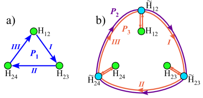
Figure 5: Braiding paths in Hamiltonian space. (a) Path $P_{1}$, for which we compute the braiding adiabatic evolution operator explicitly. (b) A different path $P_{2}$, whose Hamiltonians at the intermediate stages are assumed to be adiabatically connectable to those of $P_{1}$. $P_{3}$ is a path equivalent to $P_{2}$, in which each intermediate Hamiltonian of $P_{2}$ evolves to the corresponding Hamiltonian of $P_{1}$ and then back.

In order to make this argument more formal, let us define $P_{1}$ as the closed path in Hamiltonian space, $H_{12}\rightarrow H_{23}\rightarrow H_{24}\rightarrow H_{12}$, for which we computed the evolution operator. ($P_{1}$ is summarized in Table 1.) Suppose that we replace $P_{1}$ by a different, “realistic” path $P_{2}$, defined as $\tilde{H}_{12}\rightarrow\tilde{H}_{23}\rightarrow\tilde{H}_{24}\rightarrow\tilde{H}_{12}$, which has the same symmetries as those of the original trajectory in each stage (Table 1). $P_{1}$ and $P_{2}$ are represented in Fig. 5 a and b, respectively. We assume further that the Hamiltonian at the end of every stage of $P_{2}$ is adiabatically connectable to that of the original path $P_{1}$, e.g. $\tilde{H}_{12}$ and $H_{12}$ are adiabatically connectable, etc. We argue that the adiabatic evolution associated with $P_{2}$ is unitarily equivalent to that of $P_{1}$. To show this, consider the modified path $P_{3}$ shown in Fig. 5:

$$H_{12} \rightarrow\tilde{H}_{12}\rightarrow\tilde{H}_{23}\rightarrow H_{23}\rightarrow\tilde{H}_{23}$$

$$\rightarrow \tilde{H}_{24}\rightarrow H_{24}\rightarrow\tilde{H}_{24}\rightarrow\tilde{H}_{12}\rightarrow H_{12}.$$ (73)

Clearly, Eq. (73) can be viewed as a deformed version of the original trajectory $P_{1}$, in which the intermediate Hamiltonian during each stage is deformed relative to the original trajectory of Table 1. Since the intermediate Hamiltonian in every stage of trajectory (73) has the same symmetries as those of the original trajectory, the analysis outlined in the previous section shows that the evolution operator representing the overall trajectory (73) is $e^{i\omega}\hat{U}_{34}$, where $\omega$ is global phase factor.

On the other hand, we can consider $P_{3}$ starting and ending with $\tilde{H}_{12}$, as the “realistic” trajectory $P_{2}$. Since for example, the step $\tilde{H}_{23}\rightarrow H_{23}$ is “undone” by the next step $H_{23}\rightarrow\tilde{H}_{23}$, $P_{2}$ is unitarily related to the $P_{3}$ by $e^{i\omega}V\hat{U}_{34}V^{{\dagger}}$, where $V$ represents the evolution from $\tilde{H}_{12}$ to $H_{12}$. In essence, the matrix $V$ relates the eigenstates of the “realistic” initial Hamiltonian $\tilde{H}_{12}$, to those of $H_{12}$. We conclude that the adiabatic evolutions corresponding to paths $P_{1}$ and $P_{2}$ are physically equivalent, and therefore the braiding operation is robust to changes in the path in Hamiltonian space, as long as the conditions $1-3$ listed above are met.

C.2 Symmetries of the Hamiltonian during the braiding process

Next, we discuss the symmetry requirements in every stage in more physical terms. The topological stability of the braiding operation depends crucially on the symmetries of the Hamiltonian throughout the different stages of the braiding operation. We now argue that these symmetry properties are largely independent of the microscopic details of the Hamiltonian in each stage. This is since the definition of the braid operation only contains information regarding which interfaces are brought in proximity at each stage. For instance, any Hamiltonian trajectory corresponding to this braid operation only couples interfaces $1$, $2$ and $3$ during stage I (see Fig. 2). Any such Hamiltonian necessarily commutes with $e^{i\pi\hat{S}_{3}}$ and $e^{i\pi\hat{Q}_{3}}$, independently of its microscopic details. For example, adding terms such as higher powers of $\chi_{2,\uparrow}\chi_{1,\uparrow}^{\dagger}$, retains these symmetries. Likewise, terms representing direct coupling between interfaces $1$ and $3$, such as powers of $\chi_{3,\uparrow}\chi_{1,\uparrow}^{\dagger}$ can be added, as long as they are absent at the beginning and end of stage I, when interfaces $1$ and $3$ are far apart.

A similar statement can be made for stage II: as long as interfaces $5$, $6$, and $1$ remain decoupled throughout the evolution, the Hamiltonian necessarily maintains the same symmetries as those in in Table 1, regardless of the microscopic details of the process.

The symmetry requirement in stage III requires more care. At this stage, interfaces $1$,$2$ and $4$ are coupled. Crucially, we note that the commutation relations in Eq. (12) give $\left[\chi_{i\downarrow},\chi_{j\uparrow}\chi^{{\dagger}}_{k\uparrow}\right]=0$ for any $j,k\neq i$. Therefore, as long as we allow tunneling of only spin-up particles between interfaces $1$,$2$ and $4$, we are assured that $\chi_{3,\downarrow}$ commutes with the Hamiltonian. It follows that $\chi^{\phantom{{\dagger}}}_{5,\downarrow}\chi^{{\dagger}}_{3,\downarrow}=e^{-i\pi\hat{Q}_{2}}e^{i\pi\hat{S}_{3}}$, the symmetry operator required in stage III, also commutes with the Hamiltonian. Again, this symmetry would be maintained independently of the exact form of the Hamiltonian, as long as it obeys the above restriction. The physical reason behind this symmetry is clarified by noting that transferring $n$ up-spin quasi-particles to interface $4$ (from either $1$ or $2$) changes $e^{i\pi\hat{Q}_{2}}\rightarrow e^{i\pi(\hat{Q}_{2}+\frac{n}{m})}$ and $e^{i\pi\hat{S}_{3}}\rightarrow e^{i\pi(\hat{S}_{3}+\frac{n}{m})}$, leaving $e^{-i\pi\hat{Q}_{2}}e^{i\pi\hat{S}_{3}}$ invariant.

We now see why it is crucial, in order to allow for the braiding operation, to have only one species of quasi-particles tunnelling between interfaces. If quasi-particles of both spins are allowed to tunnel, $e^{-i\pi\hat{Q}_{2}}e^{i\pi\hat{S}_{3}}$ would cease to be a good symmetry - in fact, the symmetry of the Hamiltonain is lowered, and the ground state degeneracy is reduced from $\left(2m\right)$ to just $2$, violating the adiabatically of the braiding process. This is a special property of the fractional ($m>1$) case; for $m=1$, there is no difference between up and down quasiparticle tunneling.

We note that the restriction to single species tunneling was unnecessary in stages I and II, which retain the same symmetries even when both spin species are allowed to tunnel. Moreover, if we allowed only spin down quasi-particles to tunnel between $2$ and $4$, there would be an alternative symmetry operator $e^{i\pi\hat{Q}_{2}}e^{i\pi\hat{S}_{3}}$ at stage III. The braid operation with this type of coupling would yield a unitary operator of the same form found in Sec VI.

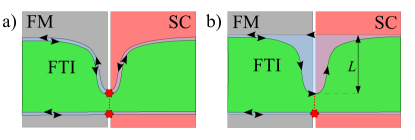
Figure 6: Constrictions in an FTI bar. We view the FTI as a combination of two FQH droplets with opposite spins and opposite filling fractions. The arrows show the direction of propagation of the edge states of the two FQH bars. The red stars mark the position of the SC/FM interfaces on the edges. (a) Constriction created by a gate potential, which acts on both spin species. In this case, quasi-particles of both spin species can tunnel across the constriction. (b) Applying a local Zeeman field splits the spin up and spin down edge states, such that only one spin species can tunnel across the constriction.

The restriction of single spin species tunnelling can be met in the different realizations of the model analyzed above. First, consider the realization using a fractional quantum Hall liquid, in which an insulating trench separates two counter propagating edge states (Fig. 1b). In this realization, the labels spin up and down indicate whether the quasi-particles are on the inner or outer edge respectively. When we deform the system in order to put interfaces in proximity, we must specify whether this deformation shrinks the inner or outer droplet of the quantum Hall liquid. Suppose we shrink the inner droplet. Then quasi-particle tunnelling between interfaces proceeds through the inner droplet. Therefore in this case, quasi-particles can only tunnel from the inner edge at one interface location to the inner edge at another. Only electron tunneling processes are allowed between the interfaces on the outer edge. However, electron tunnelling from the outer and inner edge are equivalent, as these are related by cooper-pair tunnelling or “spin flip” operators. To conclude, in this realization, choosing whether to deform the inner or outer quantum Hall droplet selects which spin species of quasi-particles are allowed to tunnel between interfaces.

Let us now consider the realization of the system on the edge of a Fractional Topological Insulator. Suppose that one can apply either ordinary gate potentials, or Zeeman fields in the $z$ direction (by coupling to a nearby ferromagnet polarized along $z$), which act as opposite gate potentials for the two spin species. Then there are two ways of coupling two interfaces, depicted in Fig. 6. One can either create a constriction in both spin species by applying an appropriate gate voltage (Fig. 6a), which allows quasi-particle tunnelling of both spin species between the interfaces across the constriction, or create a constriction for one spin species only, e.g. spin up (Fig. 6b), in which case only that spin species tunnels. Note that in the latter case, we have split the spin up and spin down edge states into two counter-propagating edge modes, which become gapless. However, if the length of the split region is $L$, there still is a finite-size gap of the order of $v_{F}/L$, where $v_{F}$ is the Fermi velocity on the edge. The tunnelling of quasi-particles of spin up across the constriction, on the other hand, is enhanced by a factor of the order of $\exp\left(L/\xi\right)$ relative to that of spin down, where $\xi$ is the correlation length in the bulk. Therefore, the tunnelling of spin up quasi-particles can, in principle, be enhanced parametrically without reducing the gap considerably.

Appendix D Yang-Baxter equations

Here, we verify that the unitaries representing braiding of two neighboring interfaces by tunneling of quasi-particles satisfy the Yang-Baxter equations. Imagine that we start from three consecutive interfaces, 1, 2, and 3, shown in Fig. 3. The segment between 1 and 2 is a superconducting (SC) segment, and the segment between 2 and 3 is a ferromagnetic (FM) segment. $e^{i\pi\hat{Q}}$ and $e^{i\pi\hat{S}}$ are the charge and spin operators acting on the SC and FM segments, respectively. In terms of these operators, one can express the unitary matrices that correspond to braiding (1,2) and (2,3):

$$U_{12} =e^{i\frac{\pi m}{2}\hat{Q}^{2}}=\frac{1}{\sqrt{2m}}\sum_{k=0}^{2m-1}e^{-i\frac{\pi}{2m}k^{2}+i\frac{\pi}{4}}e^{i\pi k\hat{Q}},$$

$$U_{23} =e^{i\frac{\pi m}{2}\hat{S}^{2}}=\frac{1}{\sqrt{2m}}\sum_{k=0}^{2m-1}e^{-i\frac{\pi}{2m}k^{2}+i\frac{\pi}{4}}e^{i\pi k\hat{S}}.$$ (74)

Here, we have used the expansion of the braiding matrices in terms of the spin and charge operators and their harmonics.

The Yang-Baxter equations state that

$$U_{12}U_{23}U_{12}=U_{23}U_{12}U_{23}.$$ (75)

This relation can be understood pictorially, as shown in Fig. 3. Inserting Eqs. (74) into the left hand side of (75), and using $e^{i\pi\hat{Q}}e^{i\pi\hat{S}}=e^{-i\frac{\pi}{m}}e^{i\pi\hat{S}}e^{i\pi\hat{Q}}$, we get

$$U_{12}U_{23}U_{12} =\sum_{k_{1},k_{2},k_{3}}\frac{e^{-i\frac{\pi}{2m}\left(k_{1}^{2}+k_{2}^{2}+k_{3}^{2}\right)+i\frac{3\pi}{4}}}{\left(2m\right)^{\frac{3}{2}}}e^{i\pi k_{1}\hat{Q}}e^{i\pi k_{2}\hat{S}}e^{i\pi k_{3}\hat{Q}}$$

$$=\sum_{k_{1},k_{2},k_{3}}\frac{e^{-i\frac{\pi}{2m}\left[\left(k_{1}-k_{2}\right)^{2}+k_{3}^{2}\right]+i\frac{3\pi}{4}}}{\left(2m\right)^{\frac{3}{2}}}e^{i\pi k_{2}\hat{S}}e^{i\pi\left(k_{1}+k_{3}\right)\hat{Q}}.$$ (76)

The sums over $k_{1,2,3}$ run from $0$ to $2m-1$. Changing variables $k_{2}\rightarrow k_{1}+k_{2}$, and $k_{3}\rightarrow k_{3}-k_{1}$,

$$U_{12}U_{23}U_{12} =\sum_{k_{1},k_{2},k_{3}}\frac{e^{-i\frac{\pi}{2m}\left[k_{2}^{2}+\left(k_{3}-k_{1}\right)^{2}\right]+i\frac{3\pi}{4}}}{\left(2m\right)^{\frac{3}{2}}}e^{i\pi\left(k_{1}+k_{2}\right)\hat{S}}e^{i\pi k_{3}\hat{Q}}$$

$$=\sum_{k_{1},k_{2},k_{3}}\frac{e^{-i\frac{\pi}{2m}\left(k_{1}^{2}+k_{2}^{2}+k_{3}^{2}\right)+i\frac{3\pi}{4}}}{\left(2m\right)^{\frac{3}{2}}}e^{i\pi k_{2}\hat{S}}e^{i\pi k_{3}\hat{Q}}e^{i\pi k_{1}\hat{S}}$$

$$=e^{i\frac{\pi m}{2}\hat{S}^{2}}e^{i\frac{\pi m}{2}\hat{Q}^{2}}e^{i\frac{\pi m}{2}\hat{S}^{2}}=U_{23}U_{12}U_{23}.$$ (77)

In the second line we have commuted $e^{i\pi k_{1}\hat{S}}$ with $e^{i\pi k_{3}\hat{Q}}$. This establishes the Yang-Baxter equation for the braiding matrices (74). Conjugating Eq. (75) by $e^{i\pi\hat{Q}_{L}k_{1}}e^{-i\pi\hat{S}_{R}k_{2}}$, where $e^{i\pi\hat{Q}_{L}}$ correspond to the charge in the SC segment on the left of $e^{i\pi\hat{Q}}$, and $e^{i\pi\hat{S}_{R}}$ to the spin in the FM segment on the right of $e^{i\pi\hat{S}}$, we get Eq. (27).

Appendix E More on the Braiding and Topological Spin of Boundary anyons

In Sec VII, we have derived the representation of the braid group using an analogy to braiding properties of anyons in two dimensions. The derivation proceeded using two important assumptions, and below we explain why these assumptions actually follow from properties of two dimensional anyons.

E.1 Properties of the particle exchanges

Consider a two dimensional theory, in which particle of type $a$ is exchanged first with particle of type $b$ and then with particle of type $c$. The operation should depend only on the type of particle $a$, and the total topological charge of particles $b$ and $c$. The operation should not be able to distinguish the finer splitting of the combined charge into the charges $b$ and $c$. This condition can be summarized pictorially in Fig 7.

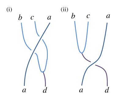
Figure 7: Properties of particle exchanges (i) Two consecutive exchanges, first between particles $a$ and $b$, and then between particles $b$ and $c$. (ii) Particle $a$ is exchanged with a particle $d$, which is the particle resulting from fusing $b$ and $c$. For two dimensional anyons, a proper definition of the braid matrix between any two particle types establishes an equality between (i) and (ii). For the case $a=b=c=X$ and $d=q$, we only use the property that the two braids in (i) move the label $q$ one segment to the left, as shown in (ii). For the case where $a=q_{1}$,$b=q_{2}$,$c=q_{3}$ and $d=q_{2}+q_{3}\mod 2m$, we show that the two sides are indeed equal

Importantly, the conditions summarized in Fig 7 hold also in our one dimensional system, for the representation derived in Sec. VII, as we shall show below. The importance of these conditions to our derivation in Sec. VII is threefold, since it can be used to (i) show that the process in Fig. 4(c) indeed exchanges the charges of the two segments; (ii) show that the TS of the $q_{1}$, $q_{2}$ composite is equal to the TS of $q_{1}+q_{2}\mod 2m$; (iii) show that the Yang-Baxter equations hold for a braid of any two particle types. Therefore, the only assumption necessary for the derivation presented in Sec. VII is that the condition summarized in Fig. 7 holds.

In the following, we shall study three important cases, for which we verify explicitly that the conditions in Fig. 7 hold in our one dimensional system. These three cases are used to verify the assumptions (i) and (ii) above.

E.1.1 $a=b=c=X,d=q$

For concreteness, Consider four neighboring interfaces $X_{1}$–$X_{4}$, flanking alternating FM, SC and FM segments. The operators corresponding to the charges in the different segments are $\chi_{3\uparrow}\chi^{{\dagger}}_{2\uparrow}={e^{i\pi\hat{Q}}}$, $\chi_{2\uparrow}\chi^{{\dagger}}_{1\uparrow}=e^{i\pi\hat{S}_{1}}$, $\chi_{3\uparrow}\chi^{{\dagger}}_{4\uparrow}=e^{i\pi\hat{S}_{2}}$. We shall also use $\chi_{4\uparrow}\chi^{{\dagger}}_{1\uparrow}=e^{i\pi\hat{S}_{1}}{e^{i\pi\hat{Q}}}e^{i\pi\hat{S}_{2}}$. Consider an initial state of the system which is an eigenstate of ${e^{i\pi\hat{Q}}}$ with eigenvalue $e^{i\frac{\pi}{m}q}$, and of $e^{i\pi\hat{S_{1}}+\hat{S_{2}}}$ with eigenvalue $e^{i\frac{\pi}{m}s_{\rm tot}}$,

$$|q,s_{\rm tot}\rangle=\frac{1}{\sqrt{2m}}\sum_{n=0}^{2m-1}e^{i\frac{\pi}{m}qn}|s_{1}=-n,s_{2}=s_{\rm tot}+n\rangle$$ (78)

where $s_{1}$ and $s_{2}$ correspond to $e^{i\pi\hat{S}_{1}}$ and $e^{i\pi\hat{S}_{2}}$. Note that such a state is also an eigenstate of $\chi_{4\uparrow}\chi^{{\dagger}}_{1\uparrow}$.

Following Fig. 7, consider two braid operations first between $X_{1}$ and $X_{2}$ and then between $X_{2}$ and $X_{3}$. Using ${e^{i\pi\hat{Q}}}|s_{1},s_{2}\rangle=|s_{1}-1,s_{2}+1\rangle$, and the Fourier representation of the braid operators, the resulting state is

$$(2m)\,e^{-i\frac{\pi}{2}}U_{12}(\hat{Q})U_{23}(\hat{S_{1}})|q,s_{\rm tot}\rangle$$

$$= \sum_{n,p,k=0}^{2m-1}e^{i\frac{\pi}{2m}\left[-\left(p^{2}+k^{2}\right)+2qn-2np\right]}|-n-k,s_{\rm tot}+n+k\rangle$$

Denoting $l=n+k$ we arrive at

$$(2m)\,e^{-i\frac{\pi}{2}}U_{12}(\hat{Q})U_{23}(\hat{S_{1}})|q,s_{\rm tot}\rangle$$

$$= \sum_{n,p,l=0}^{2m-1}e^{i\frac{\pi}{2m}\left[-\left((p+n)^{2}+l^{2}\right)+2(q+l)n\right]}|-l,s_{\rm tot}+l\rangle$$

and therefore

$$(2m)\,e^{-i\frac{\pi}{2}}U_{12}(\hat{Q})U_{23}(\hat{S_{1}})|q,s_{\rm tot}\rangle$$

$$= \left(\sum_{r=0}^{2m-1}e^{-i\frac{\pi}{2m}r^{2}}\right)e^{-i\frac{\pi}{2m}q^{2}}|s_{1}=q,s_{2}=s_{\rm tot}-q\rangle$$

We see therefore, that the two consecutive exchanges are equivalent to moving the charge $q$ one segment to the left, i.e., $e^{i\frac{\pi q}{m}}$ becomes the eigenvalue of $\chi_{2\uparrow}\chi^{{\dagger}}_{1\uparrow}=e^{i\pi\hat{S}_{1}}$.

That is exactly what is indicated in Fig. 7 (b). The state is also multiplied by a phase which depends on the gauge choices for the different basis Kitaev (2006). Importantly, note that we could have chosen to fuse $X_{1}$ with a different interface $X_{i}$ (as long as it is not between $1$ and $3$), to form a charge $\chi_{i\uparrow}\chi^{{\dagger}}_{1\uparrow}$, which would again commute with $\chi_{3\uparrow}\chi^{{\dagger}}_{2\uparrow}$. An identical analysis to the above would yield the same result, with $\chi_{i\uparrow}$ replacing $\chi_{4\uparrow}$.

E.1.2 Exchange of two $q$’s

Using the above, we would now like to show that the four exchanges depicted in Fig. 4 (c) indeed correspond to exchanging two charges $q_{1}$ and $q_{2}$. Consider four neighboring interfaces $X_{0}$–$X_{3}$, flanking alternating SC, FM, SC segments, where the initial state is $|q_{1},q_{2}\rangle$, corresponding to an eigenstate of $\chi_{1\uparrow}\chi^{{\dagger}}_{0\uparrow}=e^{i\pi\hat{Q}_{1}}$ and $\chi_{3\uparrow}\chi^{{\dagger}}_{2\uparrow}=e^{i\pi\hat{Q}_{2}}$.

Indeed, using the above results, we see that performing the exchanges $X_{1}$ with $X_{2}$, and then $X_{2}$ and $X_{3}$, would result in an eigenstate of $\chi_{2\uparrow}\chi^{{\dagger}}_{1\uparrow}={e^{i\pi\hat{S}}}$ with eigenvalue $e^{i\frac{\pi}{m}q_{2}}$. Now, performing the exchanges $X_{0}$ with $X_{1}$, and then $X_{1}$ and $X_{2}$, and again using the previous results, we see that the resulting state is an eigenstate of $\chi_{1\uparrow}\chi^{{\dagger}}_{0\uparrow}=e^{i\pi\hat{Q}_{1}}$ with eigenvalue $e^{i\frac{\pi}{m}q_{2}}$. Therefore, it is an eigenstate of $\chi_{3\uparrow}\chi^{{\dagger}}_{2\uparrow}=e^{i\pi\hat{Q}_{2}}$ with eigenvalue $e^{i\frac{\pi}{m}q_{1}}$ (the total charge in the two segments is preserved). Therefore, the two charges have been exchanged by the sequence depicted in Fig. 4 (c).

We shall now explicitly calculate the phase factor resulting from an exchange of two charges. Let us denote the operation at point by $U_{\hat{Q}_{1},\hat{Q}_{2}}$. We would now like to verify that

$$U_{\hat{Q}_{1},\hat{Q}_{2}}|q_{1},q_{2}\rangle \equiv U_{23}(\hat{S})U_{34}(\hat{Q}_{2})U_{12}(\hat{Q}_{1})U_{23}(\hat{S})|q_{1},q_{2}\rangle$$ (82)

$$= e^{i\phi(q_{1},q_{2})}|q_{2},q_{1}\rangle,$$

and find the abelian phase $\phi(q_{1},q_{2})$ associated with this exchange. The sequence of the four braid operation in the above equation corresponds to Fig 4 (c). Using ${e^{i\pi\hat{S}}}|q_{1},q_{2}\rangle=|q_{1}-1,q_{2}+1\rangle$ and the Fourier representation of the braid operators, we arrive at

$$\sum_{n,p=0}^{2m-1}e^{i\frac{\pi}{2m}\left[-\left(n^{2}+p^{2}\right)+\left(q_{1}-n\right)^{2}+\left(q_{2}+n\right)^{2}\right]}|q_{1}-n-p,q_{2}+n+p\rangle$$ (83)

Denoting $l=p+n$ we arrive at

$$\sum_{n,l=0}^{2m-1}e^{i\frac{\pi}{2m}\left[\left(-l^{2}+2nl\right)+2\left(q_{2}-q_{1}\right)n+q_{1}^{2}+q_{2}^{2}\right]}|q_{1}-l,q_{2}+l\rangle$$ (84)

The sum over $n$ forces $l=q_{1}-q_{2}$, which therefore gives

$$U_{\hat{Q}_{1},\hat{Q}_{2}}|q_{1},q_{2}\rangle=e^{i\frac{\pi}{m}q_{1}q_{2}}|q_{2},q_{1}\rangle.$$ (85)

Therefore, Eq. (82) hold, and the abelian phase for interchanging two charges $q_{1}$ and $q_{2}$ is just $e^{i\frac{\pi}{m}q_{1}q_{2}}$, which is consistent with the topological spin for the charges, $\theta_{q}=e^{i\frac{\pi}{m}q^{2}}$, Eq. (29).

E.1.3 $a=q_{1}$, $b=q_{2}$, $c=q_{3}$ $d=q_{2}+q_{3}\mod 2m$

Consider three consecutive SC segments, and an initial state $|q_{1},q_{2},q_{3}\rangle$, corresponding to an eigenstate of $e^{i\pi\hat{Q}_{1}}$,$e^{i\pi\hat{Q}_{2}}$,and $e^{i\pi\hat{Q}_{3}}$. On the left side of Fig. 7, we first have an exchange of the charge of the first and second segments, resulting, according to the above discussion, in the state $e^{i\frac{\pi}{m}q_{1}q_{2}}|q_{2},q_{1},q_{3}\rangle$, followed by an exchange of the second and third segment, resulting in $e^{i\frac{\pi}{m}\left(q_{1}q_{2}+q_{1}q_{3}\right)}|q_{2},q_{3},q_{1}\rangle$. Clearly, that is exactly the result of the operation on the left side of Fig. 7, in which the total charge $q_{2}+q_{3}$ is exchanged with $q_{1}$ and then split again into the two segments.

E.2 Consistency check

In this section we would like to verify that the topological spin of the interfaces is indeed well defined, i.e., the phase acquired by the operation defining the topological spin is independent of the initial state of the system. Consider the procedure in Fig. 4 (e). Interface $1$ flanks the left side of a SC segment, which corresponds to ${e^{i\pi\hat{Q}}}$. The initial state can be taken as an eigenstate of ${e^{i\pi\hat{Q}}}$ with eigenvalue $q$. A FM segment is nucleated to the right of it. The FM segment is nucleated with spin zero. Therefore, the state after the nucleation of this segment is

$$|\psi(q,s=0)\rangle=\frac{1}{\sqrt{2m}}\sum_{n=0}^{2m-1}|q_{1}=q-n,q_{2}=q+n\rangle$$ (86)

As explained in Sec. VII, the braid operation between interfaces $1$ and $2$ does not change the charge of the SC segment between interfaces $1$ and $2$, the charge between $3$ and $4$, and therefore the total charge $q$ (numbering increases to the right). Therefore,

$$U_{12}|\psi(q,s)\rangle=\frac{1}{\sqrt{2m}}\sum_{n=0}^{2m-1}e^{i\varphi(q-n)}|q_{1}=q-n,q_{2}=q+n\rangle$$ (87)

where we keep the phase function $\varphi(q)$ completely general. We now project on the subspace with ${e^{i\pi\hat{S}}}=1$ in the FM segment, i.e. we apply the projector

$$\Pi_{s=0}=\sum_{q}|\psi(q,s=0)\rangle\langle\psi(s=0,q)|$$ (88)

were the identity operation is implicitly assumed to act on all other degrees of freedom. Applying the projection yields (up to normalization),

$$\theta_{X}=\sum_{n=0}^{2m-1}e^{i\varphi(q-n)}.$$ (89)

Importantly, $\theta_{X}$ does not depend on $q$, as the sum runs over all possible values for charges.

References

- Leinaas and Myrheim (1977) J. M. Leinaas and J. Myrheim, Nuovo Cimento B Serie 37, 1 (1977).
- Blok and Wen (1992) B. Blok and X.-G. Wen, Nucl. Phys. B 374, 615 (1992).
- Stern (2010) A. Stern, Nature 464, 187 (2010).
- Arovas et al. (1984) D. Arovas, J. R. Schrieffer, and F. Wilczek, Physical Review Letters 53, 722 (1984).
- Kitaev (2003) A. Y. Kitaev, Annals of Physics 303, 2 (2003).
- Moore and Read (1991) G. Moore and N. Read, Nuclear Physics B 360, 362 (1991).
- Read and Rezayi (1996) N. Read and E. Rezayi, Physical Review B 54, 16864 (1996).
- Stern (2008) A. Stern, Annals of Physics 323, 204 (2008).
- Kitaev (2006) A. Kitaev, Annals of Physics 321, 2 (2006).
- Read and Green (2000) N. Read and D. Green, Physical Review B 61, 10267 (2000).
- Ivanov (2001) D. A. Ivanov, Physical Review Letters 86, 268 (2001).
- Nayak and Wilczek (1996) C. Nayak and F. Wilczek, Nucl. Phys. B 479, 529 (1996).
- Fu and Kane (2008) L. Fu and C. L. Kane, Physical Review Letters 100, 096407 (2008).
- Fu and Kane (2009) L. Fu and C. L. Kane, Physical Review B 79, 161408 (2009).
- Sau et al. (2010a) J. D. Sau, R. M. Lutchyn, S. Tewari, and S. Das Sarma, Physical Review Letters 104, 040502 (2010a).
- Qi et al. (2010) X.-L. Qi, T. L. Hughes, and S.-C. Zhang, Physical Review B 82, 184516 (2010).
- Sau et al. (2010b) J. D. Sau, S. Tewari, R. M. Lutchyn, T. D. Stanescu, and S. Das Sarma, Physical Review B 82, 214509 (2010b).
- Stanescu et al. (2010) T. D. Stanescu, J. D. Sau, R. M. Lutchyn, and S. Das Sarma, Physical Review B 81, 241310 (2010).
- Oreg et al. (2010) Y. Oreg, G. Refael, and F. von Oppen, Physical Review Letters 105, 177002 (2010).
- Lutchyn et al. (2010) R. M. Lutchyn, J. D. Sau, and S. Das Sarma, Physical Review Letters 105, 077001 (2010).
- Cook and Franz (2011) A. Cook and M. Franz, Physical Review B 84, 201105 (2011).
- Mourik et al. (2012) V. Mourik, K. Zuo, S. M. Frolov, S. R. Plissard, E. P. A. M. Bakkers, and L. P. Kouwenhoven, Science (2012), 10.1126/science.1222360.
- Willett et al. (2009) R. L. Willett, L. N. Pfeiffer, and K. W. West, PNAS 106, 8853 (2009).
- (24) S. An, P. Jiang, H. Choi, W. Kang, S. H. Simon, L. N. Pfeiffer, K. W. West, and K. W. Baldwin, arXiv:1112.3400 .
- (25) L. P. Rokhinson, X. Liu, and J. K. Furdyna, arXiv:1204.4212 .
- (26) A. Das, Y. Ronen, Y. Most, Y. Oreg, M. Heiblum, and H. Shtrikman, arXiv:1205.7073 .
- Alicea (2012) J. Alicea, (2012), arXiv:1202.1293 .
- Beenakker (2011) C. W. J. Beenakker, (2011), arXiv:1112.1950 .
- Nayak et al. (2008) C. Nayak, S. H. Simon, A. Stern, M. Freedman, and S. Das Sarma, Reviews of Modern Physics 80, 1083 (2008), and references within.
- Freedman et al. (2002) M. H. Freedman, M. J. Larsen, and Z. Wang, Commun. Math. Phys. 227, 605 (2002).
- Levin and Stern (2009) M. Levin and A. Stern, Physical Review Letters 103, 196803 (2009).
- Kane and Mele (2005) C. L. Kane and E. J. Mele, Physical Review Letters 95, 146802 (2005).
- Bernevig and Zhang (2006) B. A. Bernevig and S.-C. Zhang, Physical Review Letters 96, 106802 (2006).
- Laughlin (1983) R. B. Laughlin, Physical Review Letters 50, 1395 (1983).
- Stern et al. (2004) A. Stern, F. von Oppen, and E. Mariani, Physical Review B 70, 205338 (2004).
- Teo and Kane (2010) J. C. Y. Teo and C. L. Kane, Physical Review Letters 104, 046401 (2010).
- Alicea et al. (2011) J. Alicea, Y. Oreg, G. Refael, F. von Oppen, and M. P. A. Fisher, Nature Phys. 7, 412 (2011).
- Sau et al. (2011) J. D. Sau, D. J. Clarke, and S. Tewari, Physical Review B 84, 094505 (2011).
- Halperin et al. (2012) B. I. Halperin, Y. Oreg, A. Stern, G. Refael, J. Alicea, and F. von Oppen, Physical Review B 85, 144501 (2012).
- Wen (1990) X. G. Wen, Physical Review B 41, 12838 (1990).
- Lee and Wen (1991) D.-H. Lee and X.-G. Wen, Physical Review Letters 66, 1765 (1991).
- Bombin (2010) H. Bombin, Physical Review Letters 105, 030403 (2010).
- (43) M. Barkeshli and X.-L. Qi, arXiv:1112.3311 .
- (44) Y.-Z. You and X.-G. Wen, arXiv:1204.0113 .
- (45) P. Fendley, http://www.phys.ens.fr/ jacobsen/acfta/Fendley.pdf .
- Fradkin and Kadanoff (1980) E. Fradkin and L. P. Kadanoff, Nucl. Phys. B 170, 1 (1980).
- (47) This global phase in this identity can be proved using a Gauss sum. See, e.g., B. C. Berndt and R. J. Evans, Bull. Amer. Math. Soc. 5, 107 (1981).
- Preskill (2004) J. Preskill, Lecture notes on quantum computation (2004).
- Rowell et al. (2009) E. Rowell, R. Stong, and Z. Wang, Comm. Math. Phys 292, 343 (2009).
- Freedman et al. (2006) M. Freedman, C. Nayak, and K. Walker, Physical Review B 73, 245307 (2006).
- (51) E. Berg, N. H. Lindner, G. Refael and A. Stern, unpublished.
- Hassler et al. (2010) F. Hassler, A. R. Akhmerov, C.-Y. Hou, and C. W. J. Beenakker, New Journal of Physics 12, 125002 (2010).
- Jiang et al. (2011) L. Jiang, D. Pekker, J. Alicea, G. Refael, Y. Oreg, and F. von Oppen, Physical Review Letters 107, 236401 (2011).
- Fidkowski and Kitaev (2010) L. Fidkowski and A. Kitaev, Physical Review B 81, 134509 (2010).
- Fidkowski and Kitaev (2011) L. Fidkowski and A. Kitaev, Physical Review B 83, 075103 (2011).
- Turner et al. (2011) A. M. Turner, F. Pollmann, and E. Berg, Physical Review B 83, 075102 (2011).
- Chen et al. (2011) X. Chen, Z.-C. Gu, and X.-G. Wen, Physical Review B 84, 235128 (2011).
- Schuch et al. (2011) N. Schuch, D. Perez-Garcia, and I. Cirac, Physical Review B 84, 165139 (2011).
- Halperin (1984) B. I. Halperin, Physical Review Letters 52, 1583 (1984).
- Levin et al. (2011) M. Levin, F. J. Burnell, M. Koch-Janusz, and A. Stern, Physical Review B 84, 235145 (2011).
- Swingle et al. (2011) B. Swingle, M. Barkeshli, J. McGreevy, and T. Senthil, Physical Review B 83, 195139 (2011).
- Maciejko et al. (2010) J. Maciejko, X.-L. Qi, A. Karch, and S.-C. Zhang, Physical Review Letters 105, 246809 (2010).
- (63) J. Clarke, J. Alicea, and K. Shtengel, arXiv:1204.5479 .
- (64) M. Cheng, arXiv:1204.6084 .
- (65) A. Vaezi, arXiv:1204.6245 .