Analysis of MMSE Estimation for
Compressive Sensing of Block Sparse Signals

Abstract

Minimum mean square error (MMSE) estimation of block sparse signals from noisy linear measurements is considered. Unlike in the standard compressive sensing setup where the non-zero entries of the signal are independently and uniformly distributed across the vector of interest, the information bearing components appear here in large mutually dependent clusters. Using the replica method from statistical physics, we derive a simple closed-form solution for the MMSE obtained by the optimum estimator. We show that the MMSE is a version of the Tse-Hanly formula with system load and MSE scaled by parameters that depend on the sparsity pattern of the source. It turns out that this is equal to the MSE obtained by a genie-aided MMSE estimator which is informed in advance about the exact locations of the non-zero blocks. The asymptotic results obtained by the non-rigorous replica method are found to have an excellent agreement with finite sized numerical simulations.

I Introduction

Compressive sensing (CS) [1, 2] tackles the problem of recovering a high-dimensional sparse vector from a set of linear measurements. Typically the number of observations is much less than the number of elements in the vector of interest, making naive reconstruction attempts inefficient. In addition to being an under-determined problem, the measurements may suffer from additive noise. Under such conditions, the signal model for the noisy CS measurements can be written as

$$\vspace*{-0.1ex}\boldsymbol{y}=\boldsymbol{A}\boldsymbol{x}+\boldsymbol{n}\in\mathbb{R}^{M},\vspace*{-0.1ex}$$ (1)

where $\boldsymbol{x}\in\mathbb{R}^{N}$ is the sparse vector of interest, $\boldsymbol{A}\in\mathbb{R}^{M\times N}$ the measurement matrix, and $\boldsymbol{n}\in\mathbb{R}^{M}$ represents the measurement noise. By assumption, $M<N$ and only some of the elements of $\boldsymbol{x}$ are non-zero. The task of CS is then to infer $\boldsymbol{x}$, given $\boldsymbol{A}$, $\boldsymbol{y}$ and possibly some information about the sparsity of $\boldsymbol{x}$ and the statistics of the noise $\boldsymbol{n}$.

In this paper, the vector $\boldsymbol{x}$ is assumed to have a special block sparse structure. Such sparsity patterns have recently been found, e.g., in multiband signals and multipath communication channels (see, e.g., [3, 4, 5, 6] and references therein). More precisely, the source is considered to be $K$ block sparse so that for any realization of $\boldsymbol{x}$, its information bearing entries occur in at most $K$ non-overlapping clusters. This is markedly different from the conventional sparsity assumption in CS, where the individual non-zero components are independently and uniformly distributed over $\boldsymbol{x}$. Given the $K$ block sparse source, we study the minimum mean square error (MMSE) estimation of $\boldsymbol{x}$, assuming full knowledge of the statistics of the input $\boldsymbol{x}$ and the noise $\boldsymbol{n}$. Albeit this is an optimistic scenario for practical CS problems, it provides a lower bound on the MSE for any other reconstruction method. Also, knowing the benefits of having the statistics of the system at the estimator gives a hint how much the sub-optimum blind schemes could improve if they were to learn the parameters of the problem.

The main result of the paper is the closed-form MMSE for the CS of block sparse signals. The solution turns out to be of a particularly simple form, namely, the Tse-Hanly formula [7] where the system load and MSE are scaled by parameters that depend on the sparsity pattern of the source. This is found to be equal to the MSE obtained by a genie-aided MMSE estimator that is informed in advance the locations of the non-zero blocks. The result implies that if the statistics of the block sparse CS problem are known, the MMSE is independent of the knowledge about the positions of the non-vanishing blocks.

Finally, we remark that the analysis in the paper are obtained via the replica method (RM) from statistical physics. Albeit the RM is non-rigorous, it has been used with great success for the large system analysis of, e.g., multi-antenna systems [8, 9], code division multiple access [10, 11], vector precoding [12], iterative receivers [13] and compressed sensing [14, 15, 16, 17]. The main difference here compared to [10, 11, 9, 12, 13, 14, 15, 16, 17] is that the elements of the $K$ block sparse vector $\boldsymbol{x}$ are neither independent nor identically distributed. This requires a slight modification to the standard replica treatment, as detailed in the Appendix.

I-A Notation

The probability density function (PDF) of a random vector (RV) $\boldsymbol{x}\in\mathbb{R}^{N}$ (assuming one exists) is written as $p(\boldsymbol{x})$ and conditional densities are denoted $p(\boldsymbol{x}\mid\cdots)$. The related PDFs postulated by the estimator are denoted $q(\tilde{\boldsymbol{x}})$ and $q(\tilde{\boldsymbol{x}}\mid\cdots)$, respectively. For further discussion on the so-called generalized posterior mean estimation using true and postulated probabilities, see for example, [10, 11, 13]. We denote $\boldsymbol{y}\sim p(\boldsymbol{y})=g_{N}(\boldsymbol{y}\mid\boldsymbol{\mu};\,\boldsymbol{\Sigma})$ for a RV $\boldsymbol{y}$ that is drawn according to the $N$-dimensional Gaussian density $g_{N}(\boldsymbol{y}\mid\boldsymbol{\mu};\,\boldsymbol{\Sigma})$ with mean $\boldsymbol{\mu}\in\mathbb{R}^{N}$ and covariance $\boldsymbol{\Sigma}\in\mathbb{R}^{N\times N}$. For a vector $\boldsymbol{x}$ that is drawn according to a Gaussian mixture density, we have

$$\boldsymbol{x}\sim p(\boldsymbol{x})=\sum_{r=1}^{R}\omega_{r}g_{N}(\boldsymbol{x}\mid\boldsymbol{\mu}_{r};\,\boldsymbol{\Sigma}_{r}),$$ (2)

where the density parameters $\omega_{r}$ satisfy $\sum_{r=1}^{R}\omega_{r}=1$ and $\omega_{r}\geq 0$ for all $r=1,\ldots,R.$

We write $\boldsymbol{1}_{Q}\in\mathbb{R}^{Q}$ for the all-ones vector having $Q$ elements, and given vectors $\{\boldsymbol{d}_{r}\in\mathbb{R}^{N}\}_{r=1}^{R}$, the diagonal matrix $\boldsymbol{D}=\mathop{\rm diag\/}(\boldsymbol{d}_{1},\ldots,\boldsymbol{d}_{R})\in\mathbb{R}^{NR\times NR}$ has vector $[\boldsymbol{d}_{1}^{\mathsf{T}}\;\cdots\;\,\boldsymbol{d}_{R}^{\mathsf{T}}]^{\mathsf{T}}\in\mathbb{R}^{NR}$ on the main diagonal and zeros elsewhere. Superscript ^T denotes the transpose of a matrix.

II System Model

II-A Block Sparsity

Let $N=QR$, where $Q,R$ are positive integers, be the length of the sparse vector $\boldsymbol{x}$. Furthermore, let $\boldsymbol{x}$ be composed of $R$ equal length sub-vectors $\{\boldsymbol{x}_{r}\}_{r=1}^{R}$, that is,

$$\boldsymbol{x}=\begin{bmatrix}\boldsymbol{x}_{1}\\ \vdots\\ \boldsymbol{x}_{R}\end{bmatrix}\in\mathbb{R}^{N},\;\text{ where }\;\boldsymbol{x}_{r}=\begin{bmatrix}x_{r,1}\\ \vdots\\ x_{r,Q}\end{bmatrix}\in\mathbb{R}^{Q}.$$ (3)

Instead of considering strict block sparsity where some of the sub-vectors $\{\boldsymbol{x}_{r}\}_{r=1}^{R}$ are exactly equal to zero [3, 4, 5, 6], we let $\boldsymbol{x}$ be drawn from the Gaussian mixture density

$$p(\boldsymbol{x})=\sum_{k=1}^{K}\sum_{l=1}^{L_{k}}\omega_{k,l}g_{N}(\boldsymbol{x}\mid\boldsymbol{0};\,\boldsymbol{D}_{k,l}),$$ (4)

where $K$ is an integer,

$$L_{k}=\binom{R}{k},\quad\omega_{k}=\sum_{l=1}^{L_{k}}\omega_{k,l}\quad\text{ and }\quad\sum_{k=1}^{K}\omega_{k}=1.$$ (5)

Here $\omega_{k}$ denotes the probability of observing $k$ information bearing blocks in a realization of $\boldsymbol{x}$, $L_{k}$ the number of combinations how such $k$ blocks can be arranged in $\boldsymbol{x}$, and $\omega_{k,l}\geq 0$ the probabilities related to these arrangements. In the following, the input of (1) in the event that $\boldsymbol{x}$ is drawn according to the $(k,l)$th mixture density is denoted $\boldsymbol{x}_{k,l}$.

To impose a block sparse structure on the vector of interest, the diagonal covariance matrices in (4)

$$\boldsymbol{D}_{k,l} = \mathop{\rm diag\/}(\boldsymbol{d}^{(k,l)}_{1},\ldots,\boldsymbol{d}^{(k,l)}_{R}),\qquad l=1,\ldots,L_{k},$$ (6)

are required to be distinct for all $(k,l)\neq(k^{\prime},l^{\prime})$ and taking only two values on the block diagonals

$$\boldsymbol{d}^{(k,l)}_{r}=\boldsymbol{1}_{Q}\delta^{2}\;\text{ and }\;\boldsymbol{d}^{(k,l)}_{r}=\boldsymbol{1}_{Q}\sigma^{2}_{x},\quad\forall r,k,l.$$ (7)

Here $\delta^{2}$ and $\sigma^{2}_{x}$ represent the expected signal powers of the sparsity inducing and information bearing components, respectively. With these assumptions, the per-component variance

$$\frac{1}{N}\mathsf{E}\|\boldsymbol{x}_{k,l}\|=\frac{1}{N}\mathop{\rm tr\/}(\boldsymbol{D}_{k,l})=\frac{k}{R}\sigma^{2}_{x}+\frac{R-k}{R}\delta^{2},$$ (8)

is independent of the permutation index $l=1,\ldots,L_{k}$.

Definition 1.

Let $\sigma^{2}_{x}=1$ and assume that $\boldsymbol{x}$ is a RV with density (4). We say $\boldsymbol{x}$ is an approximately $K$ block sparse RV if $\delta^{2}\ll\sigma^{2}_{x}$ and all matrices $\{\boldsymbol{D}_{k,l}\}$ satisfy (6) – (8). If $\delta^{2}\to 0^{+}$, we simply say that $\boldsymbol{x}$ is a $K$ block sparse RV. $\diamondsuit$

II-B Posterior Mean Estimation

Let $\boldsymbol{x}$ be drawn according to (4) and assume that we observe the noisy measurements $\boldsymbol{y}$ in (1). We assume that the noise $\boldsymbol{n}\sim g_{M}(\boldsymbol{n}\mid\boldsymbol{0};\,\sigma^{2}\boldsymbol{I}_{M})$ is Gaussian and independent of the signal $\boldsymbol{x}$ and the measurement matrix $\boldsymbol{A}$. Furthermore, we let $\boldsymbol{A}$ be independent of $\boldsymbol{x}$ with independent identically distributed (IID) Gaussian entries with zero mean and variance $1/M$.

Given the above assumptions, let

$$\tilde{\boldsymbol{y}}=\boldsymbol{A}\tilde{\boldsymbol{x}}+\tilde{\boldsymbol{n}}\in\mathbb{R}^{M},$$ (9)

be the signal model postulated by the estimator. We assign the postulated densities $q(\tilde{\boldsymbol{x}})$ and $q(\tilde{\boldsymbol{n}})$ to the input and noise vectors, respectively. In the following, $q(\tilde{\boldsymbol{y}}\mid\boldsymbol{A},\tilde{\boldsymbol{x}})=q(\tilde{\boldsymbol{y}}=\boldsymbol{y}\mid\boldsymbol{A},\tilde{\boldsymbol{x}})$ means that the realizations of the postulated measurement vectors $\tilde{\boldsymbol{y}}$ match the outputs $\boldsymbol{y}$ of the true signal model (1), but it can be that the input $q(\tilde{\boldsymbol{x}})\neq p(\boldsymbol{x})$ and noise $q(\tilde{\boldsymbol{n}})\neq p(\boldsymbol{n})$ statistics are mismatched. If we define an expectation operator

$$\langle\langle\cdots\rangle\rangle_{q}\triangleq\int\cdots\,q(\tilde{\boldsymbol{x}}\mid\tilde{\boldsymbol{y}},\boldsymbol{A})\mathrm{d}\tilde{\boldsymbol{x}}=\int\cdots\frac{q(\tilde{\boldsymbol{y}}\mid\boldsymbol{A},\tilde{\boldsymbol{x}})q(\tilde{\boldsymbol{x}})}{q(\tilde{\boldsymbol{y}}\mid\boldsymbol{A})}\mathrm{d}\tilde{\boldsymbol{x}},$$ (10)

a (mismatched) MMSE estimate of $\boldsymbol{x}$ for the linear model (1), given $\boldsymbol{y},\boldsymbol{A},q(\tilde{\boldsymbol{x}})$ and $q(\tilde{\boldsymbol{y}}\mid\boldsymbol{A},\tilde{\boldsymbol{x}})$, is then simply $\langle\langle\tilde{\boldsymbol{x}}\rangle\rangle_{q}$.

Lemma 1.

The MMSE estimate of $\boldsymbol{x}$ for the signal model (1) reads $\langle\langle\tilde{\boldsymbol{x}}\rangle\rangle_{p}$, i.e., $q=p$ for all densities.

Proof:

The result follows by simple algebra and is omitted due to space constraints.

Proposition 1.

The MMSE estimate of the $K$ block sparse signal $\boldsymbol{x}$ with density (4), given noisy measurements (1), reads

$$\langle\langle\tilde{\boldsymbol{x}}\rangle\rangle_{p}=\sum_{k=1}^{K}\sum_{l=1}^{L_{k}}\frac{\omega_{k,l}p_{k,l}(\boldsymbol{y}\mid\boldsymbol{A})}{p(\boldsymbol{y}\mid\boldsymbol{A})}\boldsymbol{W}_{k,l}\,\boldsymbol{y},$$ (11)

where

$$p_{k,l}(\boldsymbol{y}\mid\boldsymbol{A}) \triangleq g_{M}(\boldsymbol{y}\mid\boldsymbol{0};\,\boldsymbol{A}\boldsymbol{D}_{k,l}\boldsymbol{A}^{\mathsf{T}}+\sigma^{2}\boldsymbol{I}_{M}),$$ (12)

$$p(\boldsymbol{y}\mid\boldsymbol{A}) = \sum_{k=1}^{K}\sum_{l=1}^{L_{k}}\omega_{k,l}p_{k,l}(\boldsymbol{y}\mid\boldsymbol{A}),$$ (13)

and

$$\boldsymbol{W}_{k,l}=\boldsymbol{D}_{k,l}\boldsymbol{A}^{\mathsf{T}}\left(\boldsymbol{A}\boldsymbol{D}_{k,l}\boldsymbol{A}^{\mathsf{T}}+\sigma^{2}\boldsymbol{I}_{M}\right)^{-1}.$$ (14)

Proof:

Let $\boldsymbol{A}\in\mathbb{R}^{N\times N}$ be a symmetric positive definite matrix. Then, using Gaussian integrals

$$e^{\frac{1}{2}\boldsymbol{b}^{\mathsf{T}}\boldsymbol{A}^{-1}\boldsymbol{b}} = \sqrt{\frac{\det(\boldsymbol{A})}{2\pi^{N}}}\int e^{-\frac{1}{2}\boldsymbol{x}^{\mathsf{T}}\boldsymbol{A}\boldsymbol{x}+\boldsymbol{b}^{\mathsf{T}}\boldsymbol{x}}\mathrm{d}\boldsymbol{x},$$ (15)

$$e^{\frac{1}{2}\boldsymbol{b}^{\mathsf{T}}\boldsymbol{A}^{-1}\boldsymbol{b}}\boldsymbol{A}^{-1}\boldsymbol{b} = \sqrt{\frac{\det(\boldsymbol{A})}{2\pi^{N}}}\int\boldsymbol{x}e^{-\frac{1}{2}\boldsymbol{x}^{\mathsf{T}}\boldsymbol{A}\boldsymbol{x}+\boldsymbol{b}^{\mathsf{T}}\boldsymbol{x}}\mathrm{d}\boldsymbol{x},$$ (16)

where $\boldsymbol{x},\boldsymbol{b}\in\mathbb{R}^{N}$ on Lemma 1, along with the identities

$$\boldsymbol{I}-\boldsymbol{U}\left(\boldsymbol{B}^{-1}+\boldsymbol{V}\boldsymbol{U}\right)^{-1}\boldsymbol{V}=\left(\boldsymbol{I}+\boldsymbol{U}\boldsymbol{B}\boldsymbol{V}\right)^{-1},$$ (17)

$$\det\big{(}\boldsymbol{C}^{-1}+\boldsymbol{U}\boldsymbol{V}^{\mathsf{T}}\big{)}=\det\big{(}\boldsymbol{I}+\boldsymbol{V}^{\mathsf{T}}\boldsymbol{C}^{-1}\boldsymbol{U}\big{)}\det\big{(}\boldsymbol{C}^{-1}\big{)},$$ (18)

where all matrices are assumed to be of proper size and $\boldsymbol{B},\boldsymbol{C}$ invertible, yields Proposition 1.

Given the MMSE estimate of Proposition 1, we are now interested in computing the per-component MSE

$$\mathsf{mse}(\sigma^{2})=\mathsf{E}\|\boldsymbol{x}-\langle\langle\tilde{\boldsymbol{x}}\rangle\rangle_{p}\|^{2}/N,$$ (19)

when the dimensions of $\boldsymbol{A}$ grow large with fixed ratio $\beta=N/M$, and the number of blocks $R=N/Q$ stays finite. The desired result is obtained in two steps: 1) the replica method is used in Sec. III-A to show that the original problem can be transformed to a set of simpler ones in the large system limit; 2) the solutions to the transformed problems are given in Sec. III-B.

III Main Results

III-A Equivalent AWGN Channel

Let the indexes $k=1,\ldots,K$ and $l=1,\ldots,L_{k}$ be as in the previous section. Define a set of additive white Gaussian noise (AWGN) channels for all $k$ and $l$

$$\boldsymbol{z}_{k,l}=\boldsymbol{x}_{k,l}+\xi_{k,l}\boldsymbol{\boldsymbol{\eta}}\in\mathbb{R}^{N},\quad\boldsymbol{\boldsymbol{\eta}}\sim g_{N}(\boldsymbol{\boldsymbol{\eta}}\mid\boldsymbol{0};\,\boldsymbol{I}_{N}),$$ (20)

where $\boldsymbol{x}_{k,l}$ is a zero-mean Gaussian RV with covariance $\boldsymbol{D}_{k,l}$ and $\xi_{k,l}>0$. Let the events of observing the $(k,l)$th channel (20) be independent and occur with probability $\omega_{k,l}$ for all $k$ and $l$. Furthermore, let

$$\langle\cdots\rangle_{q}^{(k,l)} \triangleq \int\cdots\,q(\tilde{\boldsymbol{x}}_{k,l}\mid\boldsymbol{z}_{k,l})\mathrm{d}\tilde{\boldsymbol{x}}_{k,l}$$ (21)

$$= \int\cdots\frac{q(\boldsymbol{z}_{k,l}\mid\tilde{\boldsymbol{x}}_{k,l})q(\tilde{\boldsymbol{x}}_{k,l})}{q(\boldsymbol{z}_{k,l})}\mathrm{d}\tilde{\boldsymbol{x}}_{k,l},$$

be an expectation operator similar to (10), but related to the $(k,l)$th AWGN channel (20). The MMSE estimate of $\boldsymbol{x}_{k,l}$ given the channel outputs $\boldsymbol{z}_{k,l}$ is then given by

$$\langle\tilde{\boldsymbol{x}}_{k,l}\rangle_{p}^{(k,l)}=\boldsymbol{D}_{k,l}\left(\boldsymbol{D}_{k,l}+\xi^{2}_{k,l}\boldsymbol{I}_{N}\right)^{-1}\boldsymbol{z}_{k,l}.$$ (22)

We denote the per-component MSE of the estimates $\langle\tilde{\boldsymbol{x}}_{k,l}\rangle_{p}^{(k,l)}$

$$\mathsf{mse}_{\mathsf{eq}}^{(k,l)}(\xi^{2}_{k,l})=\mathsf{E}\big{\{}\|\boldsymbol{x}_{k,l}\|^{2}-\mathsf{E}\|\langle\tilde{\boldsymbol{x}}_{k,l}\rangle^{(k,l)}_{p}\|^{2}\big{\}}/N,$$ (23)

where the expectation is w.r.t the joint distribution of all variables associated with (20). The per-component MSE averaged over the realizations of the channels (20) is thus

$$\mathsf{mse}_{\mathsf{eq}}(\{\xi^{2}_{k,l}\})=\sum_{k=1}^{K}\sum_{l=1}^{L_{k}}\omega_{k,l}\mathsf{mse}_{\mathsf{eq}}^{(k,l)}(\xi^{2}_{k,l}).$$ (24)

Claim 1.

Let $\boldsymbol{x}$ be (approximately) $K$ block sparse as given in Definition 1. In the large system limit when $M,N,Q\to\infty$ with finite and fixed ratios $\beta=N/M$ and $R=N/Q$,

$$\mathsf{mse}(\sigma^{2})\to\mathsf{mse}_{\mathsf{eq}}(\{\xi^{2}_{k,l}\}),$$ (25)

where $\mathsf{mse}(\sigma^{2})$ is given in (19) and $\mathsf{mse}_{\mathsf{eq}}(\{\xi^{2}_{k,l}\})$ in (24). The noise variance $\xi^{2}_{k,l}>0$, on the other hand, is the solution to the fixed point equation

$$\xi^{2}_{k,l} = \sigma^{2}+\beta\,\mathsf{mse}_{\mathsf{eq}}^{(k,l)}(\xi^{2}_{k,l}),$$ (26)

for all $k$ and $l$.

Proof:

The proof is based on the replica method (see, e.g., [10, 11, 9, 8, 12, 13, 14, 15, 16, 17] for similar results in communication theory and signal processing) from statistical physics. The main difference to the standard approach is that here the elements of the input vector $\boldsymbol{x}$ are neither independent nor identically distributed. Thus, the decoupling result proved for the CDMA systems [11] cannot be straightforwardly extended to our case. Alternative derivation is sketched below and in part in the Appendix.

To start, let us define a modified partition function related to the posterior mean estimator (10) as [19]

$$Z(\boldsymbol{y},\boldsymbol{A},\boldsymbol{\lambda})=\int\e^{\boldsymbol{\lambda}^{\mathsf{T}}\tilde{\boldsymbol{x}}}q(\boldsymbol{y}\mid\boldsymbol{A},\tilde{\boldsymbol{x}})q(\tilde{\boldsymbol{x}})\mathrm{d}\tilde{\boldsymbol{x}},$$ (27)

where $\boldsymbol{\lambda}\in\mathbb{R}^{N}$ is a constant vector. The posterior mean estimator of $\boldsymbol{x}$ given in (10) can then be written as the gradient with respect to (w.r.t) $\boldsymbol{\lambda}$ at $\boldsymbol{\lambda}=\boldsymbol{0}$ of the free energy, i.e.,

$$\langle\langle\tilde{\boldsymbol{x}}\rangle\rangle_{q} = \nabla_{\boldsymbol{\lambda}}\log Z(\boldsymbol{y},\boldsymbol{A},\boldsymbol{\lambda})\Big{|}_{\boldsymbol{\lambda}=\boldsymbol{0}}.$$ (28)

Similarly, if (28) is the optimum MMSE estimate, that is $q=p$, and we denote the free energy density

$$f(\boldsymbol{y},\boldsymbol{A},\boldsymbol{\lambda})=\frac{1}{N}\log Z(\boldsymbol{y},\boldsymbol{A},\boldsymbol{\lambda}),$$ (29)

the average per-component MMSE is given by

$$\mathsf{mse}=\mathop{\rm tr\/}\Big{(}\mathsf{E}\big{\{}\nabla_{\boldsymbol{\lambda}\boldsymbol{\lambda}}^{2}\,f(\boldsymbol{y},\boldsymbol{A},\boldsymbol{\lambda})\big{|}_{\boldsymbol{\lambda}=\boldsymbol{0}}\big{\}}\Big{)},$$ (30)

where the expectations are w.r.t. the joint density of $(\boldsymbol{y},\boldsymbol{A})$. Unlike in [19], however, direct computation of the free energy (density) is not possible here. We thus resort to the non-rigorous RM to calculate (29) and then use the relation (30) to obtain the final result. The details are given in the Appendix.

III-B Performance of MMSE Estimation of Block Sparse Signals

Claim 1 asserts that the MSE of the estimator (11) in the original setting (1) can be obtained in the large system limit from (24). Given the Claim 1 holds, a bit of algebra gives the following proposition.

Proposition 2.

Let $\sigma^{2}_{x}=1$, $\xi^{2}_{k,l}>0$ and $N\to\infty$. Then the per-component MSE (23) is given by

$$\mathsf{mse}_{\mathsf{eq}}^{(k,l)}(\xi^{2}_{k,l})=\frac{k}{R}\frac{\xi^{2}_{k,l}}{\xi^{2}_{k,l}+1}+\frac{R-k}{R}\frac{\delta^{2}\xi^{2}_{k,l}}{\xi^{2}_{k,l}+\delta^{2}},$$ (31)

where $\xi^{2}_{k,l}$ is the solution of (26). When the source is strictly block sparse, that is $\delta^{2}\to 0^{+}$,

$$\xi^{2}_{k}\overset{\delta^{2}\to 0^{+}}{=}\frac{1}{2}\big{(}-1+\beta_{k}+\sigma^{2}+\sqrt{4\sigma^{2}+(-1+\beta_{k}+\sigma^{2})^{2}}\,\big{)},$$ (32)

where $\xi^{2}_{k}=\xi^{2}_{k,l}\;\forall l=1,\ldots,L_{k}$ and we denoted $\beta_{k}=\frac{k}{R}\beta$ for notational convenience. Thus, given Claim 1 holds, the MMSE of the block sparse system is given by

$$\mathsf{mse}(\sigma^{2})=\sum_{k=1}^{K}\omega_{k}\frac{k}{R}\frac{\xi^{2}_{k}}{\xi^{2}_{k}+1},$$ (33)

in the large system limit.

Remark 1.

Note that the MSE is independent of the distribution $\{\omega_{k,l}\}_{l}^{L_{k}}$ that makes up $\omega_{k}$ (see (5)). $\diamondsuit$

Remark 2.

As $\delta^{2}\to 0^{+}$, the noise variance (32) becomes the Tse-Hanly solution [7] for equal power users but with a modified user load $\beta_{k}=\frac{k}{R}\beta$. The same noise variance is obtained by a genie-aided MMSE receiver, conditioned on the event that $\boldsymbol{x}$ is sampled from one of the $L_{k}$ mixtures indexed by $k$. The MSE (33), on the other hand, is a summation of the related MSEs but weighted with the probability of having $k$ non-zero blocks in a realization of the source vector $\boldsymbol{x}$. Thus, there is no loss in not knowing the positions of the zero blocks in advance if we use the optimum MMSE receiver for very large $K$ block sparse systems. Note that the equivalent AWGN channel model in Sec. III-A already implies this point. For practical settings with finite sized sensing matrices, however, this does not strictly hold. $\diamondsuit$

Corollary 1.

The MMSE estimator (11) has the same MSE in the large system limit as a genie-aided MMSE estimator that knows in advance the positions of the non-zero blocks in $\boldsymbol{x}$.

To empirically verify the analytical results, we have plotted in Fig. 1 the MSE of estimator (11), obtained via computer simulations. The theoretical MSE given in Proposition 2 is given as well. In all simulation cases we have set $\omega_{k,l}=\omega=1/\sum_{k=1}^{K}L_{k}$ so that $\omega_{k}=\omega L_{k}$. For the selected cases the theory matches Monte Carlo simulations very well.

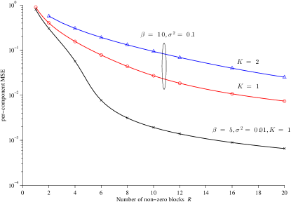
Figure 1: Per-component MMSE for the CS of block sparse signal. Solid lines are obtained from Proposition 2 with $\delta^{2}\to 0^{+}$ and markers depict numerical Monte Carlo simulations where $\sigma^{2}_{x}=1$, $\delta^{2}=10^{-6}$ and $N=1200$.

IV Conclusions

Minimum mean square error estimation of block sparse signals from noisy linear measurements was considered. The main result of the paper is the closed-form MMSE for the CS of such signals. The solution turned out to be of a particularly simple form, namely, the Tse-Hanly formula with a scaling by parameters that depend on the sparsity pattern of the source. The result implies that if the statistics of the block sparse CS problem are known, the MMSE is independent of the knowledge about the positions of the non-vanishing blocks.

[Derivation of Claim 1]

Let us assume that the free energy density (29) is self-averaging w.r.t. the quenched randomness $(\boldsymbol{A},\boldsymbol{y})$ in the large system limit $N\to\infty$. Then (29) can be written as

$$f = \lim_{N\to\infty}\frac{1}{N}\lim_{u\to 0}\frac{\partial}{\partial u}\log\mathsf{E}_{\boldsymbol{y},\boldsymbol{A}}\{Z(\boldsymbol{y},\boldsymbol{A},\boldsymbol{\lambda})^{u}\},$$ (34)

where $u$ is a real parameter. The replica trick consists of treating $u$ as an integer while calculating the expectations, but taking the limit as if $u$ was real valued outside the expectation. The second step is to exchange the limits and write the power of $u$ inside the expectation using the set $\{\boldsymbol{x}_{[a]}\}_{a=1}^{u}$ of replicated random vectors, resulting to,

$$f_{\mathsf{rm}} = \lim_{u\to 0}\frac{\partial}{\partial u}\lim_{N\to\infty}\frac{1}{N}\log\Xi^{(u)}_{N}(\boldsymbol{\lambda}),$$ (35)

where $\boldsymbol{x}_{[a]}$ are IID with density $p(\boldsymbol{x})$ and

$$\Xi^{(u)}_{N}(\boldsymbol{\lambda})=\mathsf{E}_{\boldsymbol{y},\boldsymbol{A}}\left\{\int\prod_{a=1}^{u}p(\boldsymbol{x}_{[a]})\e^{\boldsymbol{\lambda}^{\mathsf{T}}\boldsymbol{x}_{[a]}}p(\boldsymbol{y}\mid\boldsymbol{A},\boldsymbol{x}_{[a]})\mathrm{d}\boldsymbol{x}_{[a]}\right\}.$$ (36)

Unfortunately, these steps are non-rigorous and there is no general proof yet under which conditions $f_{\mathsf{rm}}$ equals $f$. For more discussion and details, see, e.g., [10, 11, 9, 8, 12, 13].

Let $\boldsymbol{x}_{[0]}$ be the true vector of interest, independent of $\{\boldsymbol{x}_{[a]}\}_{a=1}^{u}$ and distributed as $\boldsymbol{x}$. Plugging $\boldsymbol{y}=\boldsymbol{A}\boldsymbol{x}_{[0]}+\boldsymbol{n}$ to (36), the average over the additive noise vector $\boldsymbol{n}\sim g_{M}(\boldsymbol{n}\mid\boldsymbol{0};\,\sigma^{2}\boldsymbol{I}_{M})$ can be assessed using (15). Furthermore, recalling that the true and postulated source vectors have GM densities (4), we obtain (LABEL:eq:AXi_1_2) at the top of the next page, where $\mathsf{E}^{(k,l)}_{\{\boldsymbol{x}_{[a]}\}}$ denotes expectation over the vectors $\boldsymbol{x}_{[a]}\sim g_{N}(\boldsymbol{x}_{[a]}\mid\boldsymbol{0};\,\boldsymbol{D}_{k,l}),a=0,1,\ldots,u$.

$$\Xi^{(u)}_{N}(\boldsymbol{\lambda}) = \bigg{[}\frac{(u+1)^{-1}}{(2\pi\sigma^{2})^{u}}\bigg{]}^{\frac{M}{2}}\sum_{k=1}^{K}\sum_{l=1}^{L_{k}}\omega_{k,l}\mathsf{E}^{(k,l)}_{\{\boldsymbol{x}_{[a]}\}}\Bigg{\{}\mathsf{E}_{\boldsymbol{A}}\Bigg{\{}\exp\bigg{(}-\frac{1}{2\sigma^{2}(u+1)}\bigg{[}\sum_{a=0}^{u}u\|\boldsymbol{A}\boldsymbol{x}_{[a]}\|^{2}-\sum_{a=0}^{u}\sum_{b\neq a}(\boldsymbol{A}\boldsymbol{x}_{[a]})^{\mathsf{T}}(\boldsymbol{A}\boldsymbol{x}_{[b]})\bigg{]}\bigg{)}\Bigg{\}}\Bigg{\}}$$

Next, let

$$\boldsymbol{v}=[(\boldsymbol{v}_{0})^{\mathsf{T}}\,\cdots\;(\boldsymbol{v}_{u})^{\mathsf{T}}]^{\mathsf{T}}\in\mathbb{R}^{M(u+1)},$$ (38)

be a RV composed of $u+1$ sub-vectors $\boldsymbol{v}_{a}=\beta^{-1/2}\boldsymbol{A}\boldsymbol{x}_{[a]}\in\mathbb{R}^{M}$. Also denote $\boldsymbol{Q}_{k,l}=\boldsymbol{Q}^{(u)}_{k,l}\otimes\boldsymbol{I}_{M}$ where $\boldsymbol{Q}^{(u)}_{k,l}\in\mathbb{R}^{(u+1)\times(u+1)}$ and the $(a,b)$th element of $\boldsymbol{Q}^{(u)}_{k,l}$ is given by $Q_{k,l}^{[a,b]}=\boldsymbol{x}_{[a]}^{\mathsf{T}}\boldsymbol{x}_{[b]}/N$ where $\boldsymbol{x}_{[a]},\boldsymbol{x}_{[b]}\sim g_{N}(\boldsymbol{x}\mid\boldsymbol{0};\,\boldsymbol{D}_{k,l})$ for all $a,b=0,1,\ldots,u$. Then, (LABEL:eq:AXi_1_2) can be written in the form

$$\Xi^{(u)}_{N}(\boldsymbol{\lambda}) = \bigg{[}\frac{(2\pi\sigma^{2})^{-u}}{u+1}\bigg{]}^{\frac{M}{2}}\sum_{k=1}^{K}\sum_{l=1}^{L_{k}}\omega_{k,l}$$ (39)

$$\times\mathsf{E}^{(k,l)}_{\{\boldsymbol{x}_{[a]}\}}\Big{\{}\mathsf{E}_{\boldsymbol{v}\sim g_{M}(\boldsymbol{v}\mid\boldsymbol{0};\,\boldsymbol{Q}_{k,l})}\Big{\{}\e^{-\frac{1}{2}\boldsymbol{v}^{\mathsf{T}}\boldsymbol{\Sigma}\boldsymbol{v}}\Big{\}}\Big{\}},$$

where $\boldsymbol{\Sigma}=(\beta/\sigma^{2})\left[\boldsymbol{I}_{u}-\boldsymbol{1}_{u}\boldsymbol{1}_{u}^{\mathsf{T}}/(1+u)\right]\in\mathbb{R}^{(u+1)\times(u+1)}$. Using (15) to integrate over the Gaussian RV $\boldsymbol{v}$ in (39) yields

$$\Xi^{(u)}_{N}(\boldsymbol{\lambda})$$

$$\;=\sum_{k=1}^{K}\sum_{l=1}^{L_{k}}\omega_{k,l}\mathsf{E}^{(k,l)}_{\{\boldsymbol{x}_{[a]}\}}\left\{\e^{N\beta^{-1}G^{(u)}(\boldsymbol{Q}^{(u)}_{k,l})}\prod_{a=1}^{u}\e^{\boldsymbol{\lambda}^{\mathsf{T}}\boldsymbol{x}_{[a]}}\right\},$$ (40)

where

$$\e^{G^{(u)}(\boldsymbol{Q}^{(u)}_{k,l})}=\sqrt{\frac{(2\pi\sigma^{2})^{-u}}{(1+u)\det(\boldsymbol{I}+\boldsymbol{\Sigma}\boldsymbol{Q}^{(u)}_{k,l})}}.$$ (41)

To compute the expectations w.r.t., $\{\boldsymbol{x}_{[a]}\}_{a=0}^{u}$ for all $k=1,\ldots,K,l=1,\ldots,L_{k}$ in (40), we write the measure of the matrix $\boldsymbol{Q}^{(u)}_{k,l}$ as

$$\mu_{N}(\boldsymbol{Q}^{(u)}_{k,l})$$

$$\;=\mathsf{E}^{(k,l)}_{\{\boldsymbol{x}_{[a]}\}}\Bigg{\{}\prod_{a=1}^{u}\e^{\boldsymbol{\lambda}^{\mathsf{T}}\boldsymbol{x}_{[a]}}\prod_{a\leq b}\delta\left(\boldsymbol{x}_{[a]}^{\mathsf{T}}\boldsymbol{x}_{[b]}=NQ_{k,l}^{[a,b]}\right)\Bigg{\}},$$ (42)

and integrate w.r.t. (42). Writing the Dirac measures in (42) in terms of (inverse) Laplace transform and invoking saddle point integration (see [12, Appendix A] for details), we get

$$\Xi^{(u)}_{N}(\boldsymbol{\lambda})=\sum_{k=1}^{K}\sum_{l=1}^{L_{k}}\omega_{k,l}\e^{NT^{(u)}_{k,l}(\boldsymbol{\lambda})},$$ (43)

where $\tilde{\boldsymbol{Q}}\vphantom{\boldsymbol{Q}}^{(u)}_{k,l}\in\mathbb{R}^{(u+1)\times(u+1)}$ is a symmetric matrix. To obtain (43), we defined an auxiliary function

$$T^{(u)}_{k,l}(\boldsymbol{\lambda})=\sup_{\boldsymbol{Q}^{(u)}_{k,l}}\Big{\{}\beta^{-1}G^{(u)}(\boldsymbol{Q}^{(u)}_{k,l})$$

$$\;-\inf_{\tilde{\boldsymbol{Q}}\vphantom{\boldsymbol{Q}}^{(u)}_{k,l}}\Big{\{}\mathop{\rm tr\/}(\boldsymbol{Q}^{(u)}_{k,l}\tilde{\boldsymbol{Q}}\vphantom{\boldsymbol{Q}}^{(u)}_{k,l})-\lim_{N\to\infty}N^{-1}\log\phi^{(u)}_{k,l}(\tilde{\boldsymbol{Q}}\vphantom{\boldsymbol{Q}}^{(u)}_{k,l},\boldsymbol{\lambda};N)\Big{\}}\bigg{\}},$$

(44)

where

$$\phi^{(u)}_{k,l}(\tilde{\boldsymbol{Q}}\vphantom{\boldsymbol{Q}}^{(u)}_{k,l},\boldsymbol{\lambda};N)$$

$$\quad=\mathsf{E}^{(k,l)}_{\{\boldsymbol{x}_{[a]}\}}\left\{\e^{\boldsymbol{\lambda}^{\mathsf{T}}\boldsymbol{x}_{[a]}}\e^{\mathop{\rm tr\/}\left[\tilde{\boldsymbol{Q}}\vphantom{\boldsymbol{Q}}^{(u)}_{k,l}\sum_{n=1}^{N}\boldsymbol{x}^{(u)}_{n}(\boldsymbol{x}^{(u)}_{n})^{\mathsf{T}}\right]}\right\},$$ (45)

denotes the moment generating function (MGF) of (42). We also wrote $\boldsymbol{x}^{(u)}_{n}=[x_{[0],n}\,\cdots\;x_{[u],n}]\in\mathbb{R}^{u+1}$, where $n=(r-1)Q+q$ for $r=1,\ldots,R$ and $q=1,\ldots,Q$ in the notation of (3).

To make the optimization problems in (44) tractable, we assume that their solutions are the replica symmetric (RS) matrices (see, e.g., [10, 11, 9, 8, 12, 13] on discussion about this assumption)

$$\boldsymbol{Q}^{*}_{k,l} = (p_{k,l}-q_{k,l})\boldsymbol{I}_{u+1}+q_{k,l}\boldsymbol{1}_{u+1}\boldsymbol{1}_{u+1}^{\mathsf{T}},$$ (46)

$$\tilde{\boldsymbol{Q}}\vphantom{\boldsymbol{Q}}^{*}_{k,l} = (\tilde{p}_{k,l}-\tilde{q}_{k,l})\boldsymbol{I}_{u+1}+\tilde{q}_{k,l}\boldsymbol{1}_{u+1}\boldsymbol{1}_{u+1}^{\mathsf{T}},$$ (47)

respectively, where $p_{k,l},q_{k,l},\tilde{p}_{k,l},\tilde{q}_{k,l}$ are real parameters. Under the RS assumption, we get the simplifications

$$\mathop{\rm tr\/}(\boldsymbol{Q}^{(u)}_{k,l}\tilde{\boldsymbol{Q}}\vphantom{\boldsymbol{Q}}^{(u)}_{k,l})=(u+1)(p_{k,l}\tilde{p}_{k,l}+uq_{k,l}\tilde{q}_{k,l})$$ (48)

$$\quad\xrightarrow{u\to 0}0,$$ (49)

and

$$G^{(u)}(p_{k,l},q_{k,l}) = -\frac{u}{2}\log[\sigma^{2}+\beta(p_{k,l}-q_{k,l})]$$ (50)

$$-\frac{u}{2}\log(2\pi\sigma^{2})-\frac{1}{2}\log(u+1)$$

$$\xrightarrow{u\to 0}0.$$ (51)

From the first extremum in (44) one obtains $\tilde{p}_{k,l}=0$ and

$$\tilde{q}_{k,l}=\left[\sigma^{2}+\beta(p_{k,l}-q_{k,l})\right]^{-1},$$ (52)

where $p_{k,l}$ and $q_{k,l}$ are left as arbitrary but fixed parameters for now. To proceed with the second optimization problem in (44), we need to evaluate the MGF (45) under the RS assumption.

Using (15) right-to-left in (45), using the RS assumption (46) – (47) and recalling that the replicas $\{\boldsymbol{x}_{[a]}\}_{a=0}^{u}$ are IID yields after some algebra

$$\phi^{(u)}_{k,l}(\tilde{q}_{k,l},\boldsymbol{\lambda};N)=C^{(u)}_{N}(\tilde{q}_{k,l})\int\mathsf{E}^{(k,l)}_{\boldsymbol{x}}\left\{g_{N}(\boldsymbol{z}_{k,l}\mid\boldsymbol{x};\,\tilde{q}_{k,l}^{-1}\boldsymbol{I}_{N})\right\}$$

$$\qquad\times\left[\mathsf{E}^{(k,l)}_{\tilde{\boldsymbol{x}}}\left\{\e^{\boldsymbol{\lambda}^{\mathsf{T}}\tilde{\boldsymbol{x}}}g_{N}(\boldsymbol{z}_{k,l}\mid\tilde{\boldsymbol{x}};\,\tilde{q}_{k,l}^{-1}\boldsymbol{I}_{N})\right\}\right]^{u}\mathrm{d}\boldsymbol{z}_{k,l},$$ (53)

where the expectations $\mathsf{E}^{(k,l)}$ are w.r.t. zero-mean Gaussian RVs with covariance $\boldsymbol{D}_{k,l}$. The normalization factor $C^{(u)}_{N}(\tilde{q}_{k,l})=\big{[}(1+u)(2\pi/\tilde{q}_{k,l})^{u}\big{]}^{N/2}$ is due the introduction of the Gaussian densities in (53). Since

$$\phi^{(u)}_{k,l}(\tilde{q}_{k,l},\boldsymbol{\lambda};N)\xrightarrow{u\to 0}1,$$ (54)

the second optimization in (44) reduces to the conditions

$$p_{k,l}=\lim_{N\to\infty}N^{-1}\,\mathsf{E}^{(k,l)}\left\{\|\boldsymbol{x}\|^{2}\right\},$$ (55)

$$q_{k,l}=\lim_{N\to\infty}N^{-1}\mathsf{E}^{(k,l)}\left\{\|\langle\tilde{\boldsymbol{x}}\rangle^{(k,l)}_{p}\|^{2}\right\},$$ (56)

when $\boldsymbol{\lambda}=\boldsymbol{0}$ and $u\to 0$. The expectations in (55) and (56) are w.r.t $\boldsymbol{z}_{k,l}$, and the independent zero-mean Gaussian RVs $\boldsymbol{x},\tilde{\boldsymbol{x}}$ with covariance $\boldsymbol{D}_{k,l}$ as in (53). We also write

$$p_{N}(\boldsymbol{z}_{k,l})=\mathsf{E}^{(k,l)}_{\tilde{\boldsymbol{x}}}\{g_{N}(\boldsymbol{z}_{k,l}\mid\tilde{\boldsymbol{x}};\,\tilde{q}_{k,l}^{-1}\boldsymbol{I}_{N})\},$$ (57)

so that

$$\langle\tilde{\boldsymbol{x}}\rangle^{(k,l)}_{p} = \frac{1}{p(\boldsymbol{z}_{k,l})}\mathsf{E}^{(k,l)}_{\tilde{\boldsymbol{x}}}\big{\{}\tilde{\boldsymbol{x}}\,g_{N}(\boldsymbol{z}_{k,l}\mid\tilde{\boldsymbol{x}};\,\tilde{q}_{k,l}^{-1}\boldsymbol{I}_{N})\big{\}}.$$ (58)

Note that (58) is the MMSE estimator of the Gaussian channel

$$\boldsymbol{z}_{k,l}=\boldsymbol{x}+\boldsymbol{\boldsymbol{\eta}}_{k,l}\in\mathbb{R}^{N},$$ (59)

when the receiver knows the correct distributions of $\boldsymbol{\boldsymbol{\eta}}_{k,l}\sim g_{N}(\boldsymbol{\boldsymbol{\eta}}\mid\boldsymbol{0};\,\tilde{q}_{k,l}^{-1}\boldsymbol{I}_{N})$ and $\boldsymbol{x}\sim g_{N}(\boldsymbol{x}\mid\boldsymbol{0};\,\boldsymbol{D}_{k,l})$. Furthermore, from (55) and (56) we get

$$\mathsf{mse}_{\mathsf{eq}}^{(k,l)}(\tilde{q}_{k,l}) = \lim_{N\to\infty}\frac{1}{N}\big{[}\mathsf{E}^{(k,l)}\{\|\boldsymbol{x}\|^{2}\}-\mathsf{E}^{(k,l)}\{\|\langle\tilde{\boldsymbol{x}}\rangle^{(k,l)}_{p}\|^{2}\}\big{]}$$ (60)

$$= p_{k,l}-q_{k,l},$$

where $\mathsf{mse}_{\mathsf{eq}}^{(k,l)}$ is the MMSE of the Gaussian channel (59).

The free energy density under the RS assumption reads

$$f_{\mathsf{rm-rs}}=\lim_{u\to 0}\frac{\partial}{\partial u}\lim_{N\to\infty}\frac{1}{N}\log\Bigg{(}\sum_{k=1}^{K}\sum_{l=1}^{L_{k}}\omega_{k,l}\e^{NT^{(u)}_{k,l}(\boldsymbol{\lambda})}\Bigg{)}.$$ (61)

Switching the order of the limits once more yields

$$f_{\mathsf{rm-rs}} = \lim_{N\to\infty}\frac{1}{N}\lim_{u\to 0}\Bigg{\{}\bigg{(}\sum_{k=1}^{K}\sum_{l=1}^{L_{k}}\omega_{k,l}\e^{NT^{(u)}_{k,l}(\boldsymbol{\lambda})}\bigg{)}^{-1}$$ (62)

$$\qquad\quad\times\bigg{[}\sum_{k=1}^{K}\sum_{l=1}^{L_{k}}\omega_{k,l}\bigg{(}\frac{\partial}{\partial u}\e^{NT^{(u)}_{k,l}(\boldsymbol{\lambda})}\bigg{)}\bigg{]}\Bigg{\}}.$$

Since

$$T^{(u)}_{k,l}(\boldsymbol{\lambda})\xrightarrow{u\to 0}0,$$ (63)

by (5) the denominator becomes just unity and can be omitted. For the latter part,

$$\frac{\partial}{\partial u}\e^{NT^{(u)}_{k,l}(\boldsymbol{\lambda})}=N\e^{NT^{(u)}_{k,l}(\boldsymbol{\lambda})}\bigg{(}\frac{\partial}{\partial u}T^{(u)}_{k,l}(\boldsymbol{\lambda})\bigg{)},$$ (64)

where the derivative is assessed

$$\lim_{u\to 0}\frac{\partial}{\partial u}T^{(u)}_{k,l}(\boldsymbol{\lambda})=-\frac{1}{2\beta}\log[\sigma^{2}+\beta(p_{k,l}-q_{k,l})]-q_{k,l}\tilde{q}_{k,l}$$

$$\qquad+\frac{1}{2}\left[1+\log(2\pi/\tilde{q}_{k,l})\right]-\frac{1}{2\beta}\log(2\pi\e\sigma^{2})$$

$$\qquad+\lim_{N\to\infty}\frac{1}{N}\int p_{N}(\boldsymbol{z}_{k,l})h_{N}(\boldsymbol{z}_{k,l},\boldsymbol{\lambda},\tilde{q}_{k,l})\mathrm{d}\boldsymbol{z}_{k,l}.$$ (65)

Note that we defined above the function

$$h_{N}(\boldsymbol{z}_{k,l},\boldsymbol{\lambda},\tilde{q}_{k,l})$$

$$\qquad\qquad\!=\log\big{(}\mathsf{E}^{(k,l)}_{\tilde{\boldsymbol{x}}}\big{\{}\e^{\boldsymbol{\lambda}^{\mathsf{T}}\tilde{\boldsymbol{x}}}g_{N}(\boldsymbol{z}_{k,l}\mid\tilde{\boldsymbol{x}};\,\tilde{q}_{k,l}^{-1}\boldsymbol{I}_{N})\big{\}}\big{)},$$ (66)

for notational convenience. Recalling (63), we finally have the RS free energy density

$$f_{\mathsf{rm-rs}}=\frac{1}{2}\big{[}1-\beta^{-1}\log(2\pi\e\sigma^{2})\big{]}$$

$$+\frac{1}{2}\sum_{k=1}^{K}\sum_{l=1}^{L_{k}}\omega_{k,l}\big{[}\log(2\pi/\tilde{q}_{k,l})+\beta^{-1}\log\tilde{q}_{k,l}-2q_{k,l}\tilde{q}_{k,l}\big{]}$$

$$+\!\lim_{N\to\infty}\frac{1}{N}\sum_{k=1}^{K}\sum_{l=1}^{L_{k}}\omega_{k,l}\!\int\!p_{N}(\boldsymbol{z}_{k,l})h_{N}(\boldsymbol{z}_{k,l},\boldsymbol{\lambda},\tilde{q}_{k,l})\mathrm{d}\boldsymbol{z}_{k,l},$$ (67)

where only the last term depends on $\boldsymbol{\lambda}$ and is relevant for the assessment of the MSE, as given in (30).

The final task is to compute $\nabla^{2}_{\boldsymbol{\lambda}\boldsymbol{\lambda}}h_{N}(\boldsymbol{z},\boldsymbol{\lambda},\xi^{2})\big{|}_{\boldsymbol{\lambda}=\boldsymbol{0}}$. First,

$$\nabla_{\boldsymbol{\lambda}}h_{N}(\boldsymbol{z}_{k,l},\boldsymbol{\lambda},\tilde{q}_{k,l})=\frac{\mathsf{E}^{(k,l)}_{\tilde{\boldsymbol{x}}}\big{\{}\tilde{\boldsymbol{x}}\e^{\boldsymbol{\lambda}^{\mathsf{T}}\tilde{\boldsymbol{x}}}g_{N}(\boldsymbol{z}_{k,l}\mid\tilde{\boldsymbol{x}};\,\tilde{q}_{k,l}^{-1}\boldsymbol{I}_{N})\big{\}}}{\mathsf{E}^{(k,l)}_{\tilde{\boldsymbol{x}}}\big{\{}\e^{\boldsymbol{\lambda}^{\mathsf{T}}\tilde{\boldsymbol{x}}}g_{N}(\boldsymbol{z}_{k,l}\mid\tilde{\boldsymbol{x}};\,\tilde{q}_{k,l}^{-1}\boldsymbol{I}_{N})\big{\}}},$$ (68)

so that the estimator (58) can also be written as

$$\langle\tilde{\boldsymbol{x}}\rangle^{(k,l)}_{p}=\nabla_{\boldsymbol{\lambda}}h_{N}(\boldsymbol{z}_{k,l},\boldsymbol{\lambda},\tilde{q}_{k,l})\big{|}_{\boldsymbol{\lambda}=\boldsymbol{0}}.$$ (69)

Proceeding similarly, after a bit of algebra we obtain the conditional covariance matrix of the error

$$\boldsymbol{E}^{(k,l)}_{N}(\boldsymbol{z}_{k,l}) = \nabla^{2}_{\boldsymbol{\lambda}}h_{N}(\boldsymbol{z}_{k,l},\boldsymbol{\lambda},\tilde{q}_{k,l})\Big{|}_{\boldsymbol{\lambda}=\boldsymbol{0}}$$ (70)

$$= \langle\tilde{\boldsymbol{x}}\tilde{\boldsymbol{x}}^{\mathsf{T}}\rangle^{(k,l)}_{p}-\langle\tilde{\boldsymbol{x}}\rangle^{(k,l)}_{p}\big{[}\langle\tilde{\boldsymbol{x}}\rangle^{(k,l)}_{p}\big{]}^{\mathsf{T}},$$

which is also the error covariance of the estimator (58). Thus, by (30), the per-component MSE of the original MMSE estimator given in Proposition 1 reads

$$\mathsf{mse}$$

$$\;=\sum_{k=1}^{K}\sum_{l=1}^{L_{k}}\omega_{k,l}\!\lim_{N\to\infty}\frac{1}{N}\mathop{\rm tr\/}\Bigg{(}\int\!p_{N}(\boldsymbol{z}_{k,l})\boldsymbol{E}^{(k,l)}_{N}(\boldsymbol{z}_{k,l})\mathrm{d}\boldsymbol{z}_{k,l}\Bigg{)},$$

which can be written due to (55), (56) and (60) as

$$\mathsf{mse}=\sum_{k=1}^{K}\sum_{l=1}^{L_{k}}\omega_{k,l}\mathsf{mse}_{\mathsf{eq}}^{(k,l)}(\tilde{q}_{k,l}),$$ (72)

completing the proof.

References

- [1] E. J. Candes, J. Romberg, and T. Tao, “Robust uncertainty principles: Exact signal reconstruction from highly incomplete frequency information,” IEEE Trans. Inform. Theory, vol. 52, no. 2, pp. 489–509, Feb. 2006.
- [2] D. L. Donoho, “Compressed sensing,” IEEE Trans. Inform. Theory, vol. 52, no. 4, pp. 1289–1306, Apr. 2006.
- [3] M. Stojnic, “ -optimization in block-sparse compressed sensing and its strong thresholds,” IEEE J. Select. Areas Commun., vol. 4, no. 2, pp. 350–357, Apr. 2010.
- [4] M. Stojnic, F. Parvaresh, and B. Hassibi, “On the reconstruction of block-sparse signals with an optimal number of measurements,” IEEE Trans. Signal Processing, vol. 57, no. 8, pp. 3075–3085, Aug. 2009.
- [5] Y. C. Eldar, P. Kuppinger, and H. Bölcskei, “Block-sparse signals: Uncertainty relations and efficient recovery,” IEEE Trans. Signal Processing, vol. 58, no. 6, pp. 3042–3054, Jun. 2010.
- [6] R. G. Baraniuk, V. Cevher, M. F. Duarte, and C. Hegde, “Model-based compressive sensing,” IEEE Trans. Inform. Theory, vol. 56, no. 4, pp. 1982–2001, Apr. 2010.
- [7] D. N. C. Tse and S. V. Hanly, “Linear multiuser receivers: Effective interference, effective bandwidth and user capacity,” IEEE Trans. Inform. Theory, vol. 45, no. 2, pp. 641–657, Mar. 1999.
- [8] A. L. Moustakas, S. H. Simon, and A. M. Sengupta, “MIMO capacity through correlated channels in the presence of correlated interferers and noise: A (not so) large analysis,” IEEE Trans. Inform. Theory, vol. 49, no. 10, pp. 2545–2561, Oct. 2003.
- [9] R. R. Müller, “Channel capacity and minimum probability of error in large dual antenna array systems with binary modulation,” IEEE Trans. Signal Processing, vol. 51, no. 11, pp. 2821–2828, Nov. 2003.
- [10] T. Tanaka, “A statistical-mechanics approach to large-system analysis of CDMA multiuser detectors,” IEEE Trans. Inform. Theory, vol. 48, no. 11, pp. 2888–2910, Nov. 2002.
- [11] D. Guo and S. Verdú, “Randomly spread CDMA: Asymptotics via statistical physics,” IEEE Trans. Inform. Theory, vol. 51, no. 6, pp. 1983–2010, Jun. 2005.
- [12] R. R. Müller, D. Guo, and A. Moustakas, “Vector precoding for wireless MIMO systems and its replica analysis,” IEEE J. Select. Areas Commun., vol. 26, no. 3, pp. 530–540, Apr. 2008.
- [13] M. Vehkaperä, “Statistical physics approach to design and analysis of multiuser systems under channel uncertainty,” Ph.D. dissertation, NTNU, Trondheim, Norway, Aug. 2010, on-line http://urn.kb.se/resolve?urn=urn:nbn:no:ntnu:diva-8138.
- [14] S. Rangan, A. K. Fletcher, and V. K. Goyal, “Extension of replica analysis to MAP estimation with applications to compressed sensing,” in Proc. IEEE Int. Symp. Inform. Theory, Austin, TX, USA, Jun. 13 – 18 2010, pp. 1543–1547.
- [15] D. Guo, D. Baron, and S. Shamai, “A single-letter characterization of optimal noisy compressed sensing,” in Proc. Annual Allerton Conf. Commun., Contr., Computing, Monticello, IL, USA, Sep. 30 – Oct. 2 2009, pp. 52–59.
- [16] Y. Kabashima, T. Wadayama, and T. Tanaka, “Statistical mechanical analysis of a typical reconstruction limit of compressed sensing,” in Proc. IEEE Int. Symp. Inform. Theory, Austin, TX, USA, Jun. 13 – 18 2010, pp. 1533–1537.
- [17] T. Tanaka and J. Raymond, “Optimal incorporation of sparsity information by weighted optimization,” in Proc. IEEE Int. Symp. Inform. Theory, Austin, TX, USA, Jun. 13 – 18 2010, pp. 1598–1602.
- [18] A. Montanari, “Graphical models concepts in compressed sensing,” to appear in Compressed Sensing: Theory and Applications, Y. Eldar and G. Kutyniok (eds.), Cambridge University Press, 2011.
- [19] N. Merhav, “Optimum estimation via partition functions and information measures,” in Proc. IEEE Int. Symp. Inform. Theory, Austin, TX, USA, Jun. 13 – 18 2010, pp. 1473–1477.