EUROPEAN ORGANIZATION FOR NUCLEAR RESEARCH (CERN)

CERN-PH-EP-2012-107 LHCb-PAPER-2012-006 April 25, 2012

Measurement of the $C\!P$-violating phase $\phi_{s}$ in $\kern 2.59189pt\overline{\kern-2.59189ptB}{}^{0}_{s}\rightarrow{J\mskip-3.0mu/\mskip-2.0mu\psi\mskip 2.0mu}\pi^{+}\pi^{-}$ decays

The LHCb collaboration

Measurement of the mixing-induced $C\!P$-violating phase $\phi_{s}$ in $\kern 1.79993pt\overline{\kern-1.79993ptB}{}^{0}_{s}$ decays is of prime importance in probing new physics. Here 7421$\pm$105 signal events from the dominantly $C\!P$-odd final state ${J\mskip-3.0mu/\mskip-2.0mu\psi\mskip 2.0mu}\pi^{+}\pi^{-}$ are selected in 1 fb^-1 of $pp$ collision data collected at $\sqrt{s}=7$ TeV with the LHCb detector. A time-dependent fit to the data yields a value of $\phi_{s}=-0.019^{+0.173+0.004}_{-0.174-0.003}$ rad, consistent with the Standard Model expectation. No evidence of direct $C\!P$ violation is found.

Submitted to Physics Letters B

LHCb collaboration

R. Aaij³⁸, C. Abellan Beteta^33,n, B. Adeva³⁴, M. Adinolfi⁴³, C. Adrover⁶, A. Affolder⁴⁹, Z. Ajaltouni⁵, J. Albrecht³⁵, F. Alessio³⁵, M. Alexander⁴⁸, S. Ali³⁸, G. Alkhazov²⁷, P. Alvarez Cartelle³⁴, A.A. Alves Jr²², S. Amato², Y. Amhis³⁶, J. Anderson³⁷, R.B. Appleby⁵¹, O. Aquines Gutierrez¹⁰, F. Archilli^18,35, A. Artamonov ³², M. Artuso^53,35, E. Aslanides⁶, G. Auriemma^22,m, S. Bachmann¹¹, J.J. Back⁴⁵, V. Balagura^28,35, W. Baldini¹⁶, R.J. Barlow⁵¹, C. Barschel³⁵, S. Barsuk⁷, W. Barter⁴⁴, A. Bates⁴⁸, C. Bauer¹⁰, Th. Bauer³⁸, A. Bay³⁶, I. Bediaga¹, S. Belogurov²⁸, K. Belous³², I. Belyaev²⁸, E. Ben-Haim⁸, M. Benayoun⁸, G. Bencivenni¹⁸, S. Benson⁴⁷, J. Benton⁴³, R. Bernet³⁷, M.-O. Bettler¹⁷, M. van Beuzekom³⁸, A. Bien¹¹, S. Bifani¹², T. Bird⁵¹, A. Bizzeti^17,h, P.M. Bjørnstad⁵¹, T. Blake³⁵, F. Blanc³⁶, C. Blanks⁵⁰, J. Blouw¹¹, S. Blusk⁵³, A. Bobrov³¹, V. Bocci²², A. Bondar³¹, N. Bondar²⁷, W. Bonivento¹⁵, S. Borghi^48,51, A. Borgia⁵³, T.J.V. Bowcock⁴⁹, C. Bozzi¹⁶, T. Brambach⁹, J. van den Brand³⁹, J. Bressieux³⁶, D. Brett⁵¹, M. Britsch¹⁰, T. Britton⁵³, N.H. Brook⁴³, H. Brown⁴⁹, K. de Bruyn³⁸, A. Büchler-Germann³⁷, I. Burducea²⁶, A. Bursche³⁷, J. Buytaert³⁵, S. Cadeddu¹⁵, O. Callot⁷, M. Calvi^20,j, M. Calvo Gomez^33,n, A. Camboni³³, P. Campana^18,35, A. Carbone¹⁴, G. Carboni^21,k, R. Cardinale^19,i,35, A. Cardini¹⁵, L. Carson⁵⁰, K. Carvalho Akiba², G. Casse⁴⁹, M. Cattaneo³⁵, Ch. Cauet⁹, M. Charles⁵², Ph. Charpentier³⁵, N. Chiapolini³⁷, K. Ciba³⁵, X. Cid Vidal³⁴, G. Ciezarek⁵⁰, P.E.L. Clarke^47,35, M. Clemencic³⁵, H.V. Cliff⁴⁴, J. Closier³⁵, C. Coca²⁶, V. Coco³⁸, J. Cogan⁶, P. Collins³⁵, A. Comerma-Montells³³, A. Contu⁵², A. Cook⁴³, M. Coombes⁴³, G. Corti³⁵, B. Couturier³⁵, G.A. Cowan³⁶, R. Currie⁴⁷, C. D’Ambrosio³⁵, P. David⁸, P.N.Y. David³⁸, I. De Bonis⁴, S. De Capua^21,k, M. De Cian³⁷, J.M. De Miranda¹, L. De Paula², P. De Simone¹⁸, D. Decamp⁴, M. Deckenhoff⁹, H. Degaudenzi^36,35, L. Del Buono⁸, C. Deplano¹⁵, D. Derkach^14,35, O. Deschamps⁵, F. Dettori³⁹, J. Dickens⁴⁴, H. Dijkstra³⁵, P. Diniz Batista¹, F. Domingo Bonal^33,n, S. Donleavy⁴⁹, F. Dordei¹¹, A. Dosil Suárez³⁴, D. Dossett⁴⁵, A. Dovbnya⁴⁰, F. Dupertuis³⁶, R. Dzhelyadin³², A. Dziurda²³, S. Easo⁴⁶, U. Egede⁵⁰, V. Egorychev²⁸, S. Eidelman³¹, D. van Eijk³⁸, F. Eisele¹¹, S. Eisenhardt⁴⁷, R. Ekelhof⁹, L. Eklund⁴⁸, Ch. Elsasser³⁷, D. Elsby⁴², D. Esperante Pereira³⁴, A. Falabella^16,e,14, C. Färber¹¹, G. Fardell⁴⁷, C. Farinelli³⁸, S. Farry¹², V. Fave³⁶, V. Fernandez Albor³⁴, M. Ferro-Luzzi³⁵, S. Filippov³⁰, C. Fitzpatrick⁴⁷, M. Fontana¹⁰, F. Fontanelli^19,i, R. Forty³⁵, O. Francisco², M. Frank³⁵, C. Frei³⁵, M. Frosini^17,f, S. Furcas²⁰, A. Gallas Torreira³⁴, D. Galli^14,c, M. Gandelman², P. Gandini⁵², Y. Gao³, J-C. Garnier³⁵, J. Garofoli⁵³, J. Garra Tico⁴⁴, L. Garrido³³, D. Gascon³³, C. Gaspar³⁵, R. Gauld⁵², N. Gauvin³⁶, M. Gersabeck³⁵, T. Gershon^45,35, Ph. Ghez⁴, V. Gibson⁴⁴, V.V. Gligorov³⁵, C. Göbel⁵⁴, D. Golubkov²⁸, A. Golutvin^50,28,35, A. Gomes², H. Gordon⁵², M. Grabalosa Gándara³³, R. Graciani Diaz³³, L.A. Granado Cardoso³⁵, E. Graugés³³, G. Graziani¹⁷, A. Grecu²⁶, E. Greening⁵², S. Gregson⁴⁴, B. Gui⁵³, E. Gushchin³⁰, Yu. Guz³², T. Gys³⁵, C. Hadjivasiliou⁵³, G. Haefeli³⁶, C. Haen³⁵, S.C. Haines⁴⁴, T. Hampson⁴³, S. Hansmann-Menzemer¹¹, R. Harji⁵⁰, N. Harnew⁵², J. Harrison⁵¹, P.F. Harrison⁴⁵, T. Hartmann⁵⁵, J. He⁷, V. Heijne³⁸, K. Hennessy⁴⁹, P. Henrard⁵, J.A. Hernando Morata³⁴, E. van Herwijnen³⁵, E. Hicks⁴⁹, K. Holubyev¹¹, P. Hopchev⁴, W. Hulsbergen³⁸, P. Hunt⁵², T. Huse⁴⁹, R.S. Huston¹², D. Hutchcroft⁴⁹, D. Hynds⁴⁸, V. Iakovenko⁴¹, P. Ilten¹², J. Imong⁴³, R. Jacobsson³⁵, A. Jaeger¹¹, M. Jahjah Hussein⁵, E. Jans³⁸, F. Jansen³⁸, P. Jaton³⁶, B. Jean-Marie⁷, F. Jing³, M. John⁵², D. Johnson⁵², C.R. Jones⁴⁴, B. Jost³⁵, M. Kaballo⁹, S. Kandybei⁴⁰, M. Karacson³⁵, T.M. Karbach⁹, J. Keaveney¹², I.R. Kenyon⁴², U. Kerzel³⁵, T. Ketel³⁹, A. Keune³⁶, B. Khanji⁶, Y.M. Kim⁴⁷, M. Knecht³⁶, R.F. Koopman³⁹, P. Koppenburg³⁸, M. Korolev²⁹, A. Kozlinskiy³⁸, L. Kravchuk³⁰, K. Kreplin¹¹, M. Kreps⁴⁵, G. Krocker¹¹, P. Krokovny¹¹, F. Kruse⁹, K. Kruzelecki³⁵, M. Kucharczyk^20,23,35,j, V. Kudryavtsev³¹, T. Kvaratskheliya^28,35, V.N. La Thi³⁶, D. Lacarrere³⁵, G. Lafferty⁵¹, A. Lai¹⁵, D. Lambert⁴⁷, R.W. Lambert³⁹, E. Lanciotti³⁵, G. Lanfranchi¹⁸, C. Langenbruch¹¹, T. Latham⁴⁵, C. Lazzeroni⁴², R. Le Gac⁶, J. van Leerdam³⁸, J.-P. Lees⁴, R. Lefèvre⁵, A. Leflat^29,35, J. Lefrançois⁷, O. Leroy⁶, T. Lesiak²³, L. Li³, L. Li Gioi⁵, M. Lieng⁹, M. Liles⁴⁹, R. Lindner³⁵, C. Linn¹¹, B. Liu³, G. Liu³⁵, J. von Loeben²⁰, J.H. Lopes², E. Lopez Asamar³³, N. Lopez-March³⁶, H. Lu³, J. Luisier³⁶, A. Mac Raighne⁴⁸, F. Machefert⁷, I.V. Machikhiliyan^4,28, F. Maciuc¹⁰, O. Maev^27,35, J. Magnin¹, S. Malde⁵², R.M.D. Mamunur³⁵, G. Manca^15,d, G. Mancinelli⁶, N. Mangiafave⁴⁴, U. Marconi¹⁴, R. Märki³⁶, J. Marks¹¹, G. Martellotti²², A. Martens⁸, L. Martin⁵², A. Martín Sánchez⁷, M. Martinelli³⁸, D. Martinez Santos³⁵, A. Massafferri¹, Z. Mathe¹², C. Matteuzzi²⁰, M. Matveev²⁷, E. Maurice⁶, B. Maynard⁵³, A. Mazurov^16,30,35, G. McGregor⁵¹, R. McNulty¹², M. Meissner¹¹, M. Merk³⁸, J. Merkel⁹, S. Miglioranzi³⁵, D.A. Milanes¹³, M.-N. Minard⁴, J. Molina Rodriguez⁵⁴, S. Monteil⁵, D. Moran¹², P. Morawski²³, R. Mountain⁵³, I. Mous³⁸, F. Muheim⁴⁷, K. Müller³⁷, R. Muresan²⁶, B. Muryn²⁴, B. Muster³⁶, J. Mylroie-Smith⁴⁹, P. Naik⁴³, T. Nakada³⁶, R. Nandakumar⁴⁶, I. Nasteva¹, M. Needham⁴⁷, N. Neufeld³⁵, A.D. Nguyen³⁶, C. Nguyen-Mau^36,o, M. Nicol⁷, V. Niess⁵, N. Nikitin²⁹, A. Nomerotski^52,35, A. Novoselov³², A. Oblakowska-Mucha²⁴, V. Obraztsov³², S. Oggero³⁸, S. Ogilvy⁴⁸, O. Okhrimenko⁴¹, R. Oldeman^15,d,35, M. Orlandea²⁶, J.M. Otalora Goicochea², P. Owen⁵⁰, B. Pal⁵³, J. Palacios³⁷, A. Palano^13,b, M. Palutan¹⁸, J. Panman³⁵, A. Papanestis⁴⁶, M. Pappagallo⁴⁸, C. Parkes⁵¹, C.J. Parkinson⁵⁰, G. Passaleva¹⁷, G.D. Patel⁴⁹, M. Patel⁵⁰, S.K. Paterson⁵⁰, G.N. Patrick⁴⁶, C. Patrignani^19,i, C. Pavel-Nicorescu²⁶, A. Pazos Alvarez³⁴, A. Pellegrino³⁸, G. Penso^22,l, M. Pepe Altarelli³⁵, S. Perazzini^14,c, D.L. Perego^20,j, E. Perez Trigo³⁴, A. Pérez-Calero Yzquierdo³³, P. Perret⁵, M. Perrin-Terrin⁶, G. Pessina²⁰, A. Petrolini^19,i, A. Phan⁵³, E. Picatoste Olloqui³³, B. Pie Valls³³, B. Pietrzyk⁴, T. Pilař⁴⁵, D. Pinci²², R. Plackett⁴⁸, S. Playfer⁴⁷, M. Plo Casasus³⁴, G. Polok²³, A. Poluektov^45,31, E. Polycarpo², D. Popov¹⁰, B. Popovici²⁶, C. Potterat³³, A. Powell⁵², J. Prisciandaro³⁶, V. Pugatch⁴¹, A. Puig Navarro³³, W. Qian⁵³, J.H. Rademacker⁴³, B. Rakotomiaramanana³⁶, M.S. Rangel², I. Raniuk⁴⁰, G. Raven³⁹, S. Redford⁵², M.M. Reid⁴⁵, A.C. dos Reis¹, S. Ricciardi⁴⁶, A. Richards⁵⁰, K. Rinnert⁴⁹, D.A. Roa Romero⁵, P. Robbe⁷, E. Rodrigues^48,51, F. Rodrigues², P. Rodriguez Perez³⁴, G.J. Rogers⁴⁴, S. Roiser³⁵, V. Romanovsky³², M. Rosello^33,n, J. Rouvinet³⁶, T. Ruf³⁵, H. Ruiz³³, G. Sabatino^21,k, J.J. Saborido Silva³⁴, N. Sagidova²⁷, P. Sail⁴⁸, B. Saitta^15,d, C. Salzmann³⁷, M. Sannino^19,i, R. Santacesaria²², C. Santamarina Rios³⁴, R. Santinelli³⁵, E. Santovetti^21,k, M. Sapunov⁶, A. Sarti^18,l, C. Satriano^22,m, A. Satta²¹, M. Savrie^16,e, D. Savrina²⁸, P. Schaack⁵⁰, M. Schiller³⁹, H. Schindler³⁵, S. Schleich⁹, M. Schlupp⁹, M. Schmelling¹⁰, B. Schmidt³⁵, O. Schneider³⁶, A. Schopper³⁵, M.-H. Schune⁷, R. Schwemmer³⁵, B. Sciascia¹⁸, A. Sciubba^18,l, M. Seco³⁴, A. Semennikov²⁸, K. Senderowska²⁴, I. Sepp⁵⁰, N. Serra³⁷, J. Serrano⁶, P. Seyfert¹¹, M. Shapkin³², I. Shapoval^40,35, P. Shatalov²⁸, Y. Shcheglov²⁷, T. Shears⁴⁹, L. Shekhtman³¹, O. Shevchenko⁴⁰, V. Shevchenko²⁸, A. Shires⁵⁰, R. Silva Coutinho⁴⁵, T. Skwarnicki⁵³, N.A. Smith⁴⁹, E. Smith^52,46, K. Sobczak⁵, F.J.P. Soler⁴⁸, A. Solomin⁴³, F. Soomro^18,35, B. Souza De Paula², B. Spaan⁹, A. Sparkes⁴⁷, P. Spradlin⁴⁸, F. Stagni³⁵, S. Stahl¹¹, O. Steinkamp³⁷, S. Stoica²⁶, S. Stone^53,35, B. Storaci³⁸, M. Straticiuc²⁶, U. Straumann³⁷, V.K. Subbiah³⁵, S. Swientek⁹, M. Szczekowski²⁵, P. Szczypka³⁶, T. Szumlak²⁴, S. T’Jampens⁴, E. Teodorescu²⁶, F. Teubert³⁵, C. Thomas⁵², E. Thomas³⁵, J. van Tilburg¹¹, V. Tisserand⁴, M. Tobin³⁷, S. Topp-Joergensen⁵², N. Torr⁵², E. Tournefier^4,50, S. Tourneur³⁶, M.T. Tran³⁶, A. Tsaregorodtsev⁶, N. Tuning³⁸, M. Ubeda Garcia³⁵, A. Ukleja²⁵, U. Uwer¹¹, V. Vagnoni¹⁴, G. Valenti¹⁴, R. Vazquez Gomez³³, P. Vazquez Regueiro³⁴, S. Vecchi¹⁶, J.J. Velthuis⁴³, M. Veltri^17,g, B. Viaud⁷, I. Videau⁷, D. Vieira², X. Vilasis-Cardona^33,n, J. Visniakov³⁴, A. Vollhardt³⁷, D. Volyanskyy¹⁰, D. Voong⁴³, A. Vorobyev²⁷, H. Voss¹⁰, R. Waldi⁵⁵, S. Wandernoth¹¹, J. Wang⁵³, D.R. Ward⁴⁴, N.K. Watson⁴², A.D. Webber⁵¹, D. Websdale⁵⁰, M. Whitehead⁴⁵, D. Wiedner¹¹, L. Wiggers³⁸, G. Wilkinson⁵², M.P. Williams^45,46, M. Williams⁵⁰, F.F. Wilson⁴⁶, J. Wishahi⁹, M. Witek²³, W. Witzeling³⁵, S.A. Wotton⁴⁴, K. Wyllie³⁵, Y. Xie⁴⁷, F. Xing⁵², Z. Xing⁵³, Z. Yang³, R. Young⁴⁷, O. Yushchenko³², M. Zangoli¹⁴, M. Zavertyaev^10,a, F. Zhang³, L. Zhang⁵³, W.C. Zhang¹², Y. Zhang³, A. Zhelezov¹¹, L. Zhong³, A. Zvyagin³⁵.

¹Centro Brasileiro de Pesquisas Físicas (CBPF), Rio de Janeiro, Brazil
²Universidade Federal do Rio de Janeiro (UFRJ), Rio de Janeiro, Brazil
³Center for High Energy Physics, Tsinghua University, Beijing, China
⁴LAPP, Université de Savoie, CNRS/IN2P3, Annecy-Le-Vieux, France
⁵Clermont Université, Université Blaise Pascal, CNRS/IN2P3, LPC, Clermont-Ferrand, France
⁶CPPM, Aix-Marseille Université, CNRS/IN2P3, Marseille, France
⁷LAL, Université Paris-Sud, CNRS/IN2P3, Orsay, France
⁸LPNHE, Université Pierre et Marie Curie, Université Paris Diderot, CNRS/IN2P3, Paris, France
⁹Fakultät Physik, Technische Universität Dortmund, Dortmund, Germany
¹⁰Max-Planck-Institut für Kernphysik (MPIK), Heidelberg, Germany
¹¹Physikalisches Institut, Ruprecht-Karls-Universität Heidelberg, Heidelberg, Germany
¹²School of Physics, University College Dublin, Dublin, Ireland
¹³Sezione INFN di Bari, Bari, Italy
¹⁴Sezione INFN di Bologna, Bologna, Italy
¹⁵Sezione INFN di Cagliari, Cagliari, Italy
¹⁶Sezione INFN di Ferrara, Ferrara, Italy
¹⁷Sezione INFN di Firenze, Firenze, Italy
¹⁸Laboratori Nazionali dell’INFN di Frascati, Frascati, Italy
¹⁹Sezione INFN di Genova, Genova, Italy
²⁰Sezione INFN di Milano Bicocca, Milano, Italy
²¹Sezione INFN di Roma Tor Vergata, Roma, Italy
²²Sezione INFN di Roma La Sapienza, Roma, Italy
²³Henryk Niewodniczanski Institute of Nuclear Physics Polish Academy of Sciences, Kraków, Poland
²⁴AGH University of Science and Technology, Kraków, Poland
²⁵Soltan Institute for Nuclear Studies, Warsaw, Poland
²⁶Horia Hulubei National Institute of Physics and Nuclear Engineering, Bucharest-Magurele, Romania
²⁷Petersburg Nuclear Physics Institute (PNPI), Gatchina, Russia
²⁸Institute of Theoretical and Experimental Physics (ITEP), Moscow, Russia
²⁹Institute of Nuclear Physics, Moscow State University (SINP MSU), Moscow, Russia
³⁰Institute for Nuclear Research of the Russian Academy of Sciences (INR RAN), Moscow, Russia
³¹Budker Institute of Nuclear Physics (SB RAS) and Novosibirsk State University, Novosibirsk, Russia
³²Institute for High Energy Physics (IHEP), Protvino, Russia
³³Universitat de Barcelona, Barcelona, Spain
³⁴Universidad de Santiago de Compostela, Santiago de Compostela, Spain
³⁵European Organization for Nuclear Research (CERN), Geneva, Switzerland
³⁶Ecole Polytechnique Fédérale de Lausanne (EPFL), Lausanne, Switzerland
³⁷Physik-Institut, Universität Zürich, Zürich, Switzerland
³⁸Nikhef National Institute for Subatomic Physics, Amsterdam, The Netherlands
³⁹Nikhef National Institute for Subatomic Physics and Vrije Universiteit, Amsterdam, The Netherlands
⁴⁰NSC Kharkiv Institute of Physics and Technology (NSC KIPT), Kharkiv, Ukraine
⁴¹Institute for Nuclear Research of the National Academy of Sciences (KINR), Kyiv, Ukraine
⁴²University of Birmingham, Birmingham, United Kingdom
⁴³H.H. Wills Physics Laboratory, University of Bristol, Bristol, United Kingdom
⁴⁴Cavendish Laboratory, University of Cambridge, Cambridge, United Kingdom
⁴⁵Department of Physics, University of Warwick, Coventry, United Kingdom
⁴⁶STFC Rutherford Appleton Laboratory, Didcot, United Kingdom
⁴⁷School of Physics and Astronomy, University of Edinburgh, Edinburgh, United Kingdom
⁴⁸School of Physics and Astronomy, University of Glasgow, Glasgow, United Kingdom
⁴⁹Oliver Lodge Laboratory, University of Liverpool, Liverpool, United Kingdom
⁵⁰Imperial College London, London, United Kingdom
⁵¹School of Physics and Astronomy, University of Manchester, Manchester, United Kingdom
⁵²Department of Physics, University of Oxford, Oxford, United Kingdom
⁵³Syracuse University, Syracuse, NY, United States
⁵⁴Pontifícia Universidade Católica do Rio de Janeiro (PUC-Rio), Rio de Janeiro, Brazil, associated to ^2
55Physikalisches Institut, Universität Rostock, Rostock, Germany, associated to <sup>11

a</sup>P.N. Lebedev Physical Institute, Russian Academy of Science (LPI RAS), Moscow, Russia
^bUniversità di Bari, Bari, Italy
^cUniversità di Bologna, Bologna, Italy
^dUniversità di Cagliari, Cagliari, Italy
^eUniversità di Ferrara, Ferrara, Italy
^fUniversità di Firenze, Firenze, Italy
^gUniversità di Urbino, Urbino, Italy
^hUniversità di Modena e Reggio Emilia, Modena, Italy
ⁱUniversità di Genova, Genova, Italy
^jUniversità di Milano Bicocca, Milano, Italy
^kUniversità di Roma Tor Vergata, Roma, Italy
^lUniversità di Roma La Sapienza, Roma, Italy
^mUniversità della Basilicata, Potenza, Italy
ⁿLIFAELS, La Salle, Universitat Ramon Llull, Barcelona, Spain
^oHanoi University of Science, Hanoi, Viet Nam

1 Introduction

Current knowledge of the Cabibbo-Kobayashi-Maskawa (CKM) matrix leads to the Standard Model (SM) expectation that the mixing-induced $C\!P$ violation phase in $\kern 1.79993pt\overline{\kern-1.79993ptB}{}^{0}_{s}$ decays proceeding via the $b\rightarrow c\overline{c}s$ transition is small and accurately predicted [1]. Therefore, new physics can be decisively revealed by its measurement. This phase denoted by $\phi_{s}$ is given in the SM by $-2\arg\left[{V_{ts}V_{tb}^{*}}/{V_{cs}V_{cb}^{*}}\right]$, where the $V_{ij}$ are elements of the CKM matrix. Motivated by a prediction in Ref. [2], the LHCb collaboration made the first observation of $\kern 1.79993pt\overline{\kern-1.79993ptB}{}^{0}_{s}\rightarrow{J\mskip-3.0mu/\mskip-2.0mu\psi\mskip 2.0mu}f_{0}(980)$, $f_{0}(980)\rightarrow\pi^{+}\pi^{-}$ [3], which was subsequently confirmed by others [4, *Abazov:2011hv, 6]. This mode is a $C\!P$-odd eigenstate and its use obviates the need to perform an angular analysis in order to determine $\phi_{s}$ [7], as is required in the ${J\mskip-3.0mu/\mskip-2.0mu\psi\mskip 2.0mu}\phi$ final state [8, 9, *CDF:2011af]. In this Letter we measure $\phi_{s}$ using the final state ${J\mskip-3.0mu/\mskip-2.0mu\psi\mskip 2.0mu}\pi^{+}\pi^{-}$ over a large range of $\pi^{+}\pi^{-}$ masses, 775$-$1550 MeV, which has been shown to be an almost pure $C\!P$-odd eigenstate [11]. We designate events in this region as $f_{\rm odd}$. This phase is the same as that measured in ${J\mskip-3.0mu/\mskip-2.0mu\psi\mskip 2.0mu}\phi$ decays, ignoring contributions from suppressed processes [12, *Fleischer:2011au].

The decay time evolutions for initial $B_{s}^{0}$ and $\kern 1.79993pt\overline{\kern-1.79993ptB}{}^{0}_{s}$ decaying into a $C\!P$-odd eigenstate, $f_{-}$, assuming only one CKM phase, are [14, *Bigi:2000yz]

$$\Gamma\left(\accentset{\scalebox{0.4}{(}\raisebox{-1.7pt}{-}\scalebox{0.4}{)}}{B}_{s}^{0}\rightarrow f_{-}\right)={\cal N}e^{-\Gamma_{s}t}\,\Bigg{\{}\frac{e^{\Delta\Gamma_{s}t/2}}{2}(1+\cos\phi_{s})+\frac{e^{-\Delta\Gamma_{s}t/2}}{2}(1-\cos\phi_{s})\pm\sin\phi_{s}\sin\left(\Delta m_{s}\,t\right)\Bigg{\}}\,,$$ (1)

where $\Delta\Gamma_{s}=\Gamma_{\rm L}-\Gamma_{\rm H}$ is the decay width difference between light and heavy mass eigenstates, $\Gamma_{s}=(\Gamma_{\rm L}+\Gamma_{\rm H})/2$ is the average decay width, $\Delta m_{s}=m_{\rm H}-m_{\rm L}$ is the mass difference, and ${\cal N}$ is a time-independent normalization factor. The plus sign in front of the $\sin\phi_{s}$ term applies to an initial $\kern 1.79993pt\overline{\kern-1.79993ptB}{}^{0}_{s}$ and the minus sign to an initial $B^{0}_{s}$ meson. The time evolution of the untagged rate is then

$$\Gamma\left(B_{s}^{0}\rightarrow f_{-}\right)+\Gamma\left(\kern 1.79993pt\overline{\kern-1.79993ptB}{}^{0}_{s}\rightarrow f_{-}\right)={\cal N}e^{-\Gamma_{s}t}\,\Bigg{\{}e^{\Delta\Gamma_{s}t/2}(1+\cos\phi_{s})+e^{-\Delta\Gamma_{s}t/2}(1-\cos\phi_{s})\Bigg{\}}\,.$$ (2)

Note that there is information in the shape of the lifetime distribution that correlates $\Delta\Gamma_{s}$ and $\phi_{s}$. In this analysis we will use samples of both flavour tagged and untagged decays. Both Eqs. 1 and 2 are invariant under the change $\phi_{s}\rightarrow\pi-\phi_{s}$ when $\Delta\Gamma_{s}\rightarrow-\Delta\Gamma_{s}$, which gives an inherent ambiguity. Recently this ambiguity has been resolved [16], so only the allowed solution with $\Delta\Gamma_{s}>0$ will be considered.

2 Data sample and selection requirements

The data sample consists of 1 fb^-1 of integrated luminosity collected with the LHCb detector [17] at 7 TeV centre-of-mass energy in $pp$ collisions at the LHC. The detector is a single-arm forward spectrometer covering the pseudorapidity range $2<\eta<5$, designed for the study of particles containing $b$ or $c$ quarks. Components include a high-precision tracking system consisting of a silicon-strip vertex detector surrounding the $pp$ interaction region, a large-area silicon-strip detector located upstream of a dipole magnet with a bending power of about $4{\rm\,Tm}$, and three stations of silicon-strip detectors and straw drift-tubes placed downstream. The combined tracking system has a momentum resolution $\delta p/p$ that varies from 0.4% at 5$\mathrm{\,Ge\kern-1.00006ptV}$ to 0.6% at 100$\mathrm{\,Ge\kern-1.00006ptV}$, and an impact parameter (IP) resolution of 20$\,\upmu\rm m$ for tracks with high transverse momentum ($p_{\rm T}$). Charged hadrons are identified using two ring-imaging Cherenkov (RICH) detectors. Photon, electron and hadron candidates are identified by a calorimeter system consisting of scintillating-pad and pre-shower detectors, an electromagnetic calorimeter and a hadronic calorimeter. Muons are identified by a muon system composed of alternating layers of iron and multiwire proportional chambers. The trigger consists of a hardware stage, based on information from the calorimeter and muon systems, followed by a software stage which applies a full event reconstruction.

Events were triggered by detecting two muons with an invariant mass within 120  MeV of the nominal ${J\mskip-3.0mu/\mskip-2.0mu\psi\mskip 2.0mu}$ mass [18]. To be considered a ${J\mskip-3.0mu/\mskip-2.0mu\psi\mskip 2.0mu}$ candidate, particles of opposite charge are required to have $p_{\rm T}$ greater than 500 MeV, be identified as muons, and form a vertex with fit $\chi^{2}$ per number of degrees of freedom less than 16. Only candidates with a dimuon invariant mass between $-$48 MeV and +43 MeV of the ${J\mskip-3.0mu/\mskip-2.0mu\psi\mskip 2.0mu}$ mass peak are selected. For further analysis the four-momenta of the dimuons are constrained to yield the ${J\mskip-3.0mu/\mskip-2.0mu\psi\mskip 2.0mu}$ mass.

For this analysis we use a Boosted Decision Tree (BDT) [19] to set the ${J\mskip-3.0mu/\mskip-2.0mu\psi\mskip 2.0mu}\pi^{+}\pi^{-}$ selection requirements. We first implement a preselection that preserves a large fraction of the signal events, including the requirements that the pions have $p_{\rm T}$ $>$ 250 MeV and be identified by the RICH. $\kern 1.79993pt\overline{\kern-1.79993ptB}{}^{0}_{s}$ candidate decay tracks must form a common vertex that is detached from the primary vertex. The angle between the combined momentum vector of the decay products and the vector formed from the positions of the primary and the $\kern 1.79993pt\overline{\kern-1.79993ptB}{}^{0}_{s}$ decay vertices (pointing angle) is required to be consistent with zero. If more than one primary vertex is found the one corresponding to the smallest IP significance of the $\kern 1.79993pt\overline{\kern-1.79993ptB}{}^{0}_{s}$ candidate is chosen.

The variables used in the BDT are the muon identification quality, the probability that the $\pi^{\pm}$ come from the primary vertex (implemented in terms of the IP $\chi^{2}$), the $p_{\rm T}$ of each pion, the $\kern 1.79993pt\overline{\kern-1.79993ptB}{}^{0}_{s}$ vertex $\chi^{2}$, the pointing angle and the $\kern 1.79993pt\overline{\kern-1.79993ptB}{}^{0}_{s}$ flight distance from production to decay vertex. For various calibrations we also analyze samples of $\kern 1.79993pt\overline{\kern-1.79993ptB}{}^{0}\rightarrow{J\mskip-3.0mu/\mskip-2.0mu\psi\mskip 2.0mu}\kern 1.99997pt\overline{\kern-1.99997ptK}{}^{*0}$, $\kern 1.99997pt\overline{\kern-1.99997ptK}{}^{*0}\rightarrow\pi^{+}K^{-}$, and its charge-conjugate. The same selections are used as for ${J\mskip-3.0mu/\mskip-2.0mu\psi\mskip 2.0mu}\pi^{+}\pi^{-}$ except for particle identification.

The BDT is trained with $\kern 1.79993pt\overline{\kern-1.79993ptB}{}^{0}_{s}\rightarrow{J\mskip-3.0mu/\mskip-2.0mu\psi\mskip 2.0mu}f_{0}(980)$ Monte Carlo events generated using Pythia [20] and the LHCb detector simulation based on Geant4 [21]. The following two data samples are used to study the background. The first contains ${J\mskip-3.0mu/\mskip-2.0mu\psi\mskip 2.0mu}\pi^{+}\pi^{+}$ and ${J\mskip-3.0mu/\mskip-2.0mu\psi\mskip 2.0mu}\pi^{-}\pi^{-}$ events with $m({J\mskip-3.0mu/\mskip-2.0mu\psi\mskip 2.0mu}\pi^{\pm}\pi^{\pm})$ within $\pm$50 MeV of the $\kern 1.79993pt\overline{\kern-1.79993ptB}{}^{0}_{s}$ mass, called the like-sign sample. The second consists of events in the $\kern 1.79993pt\overline{\kern-1.79993ptB}{}^{0}_{s}$ sideband having $m({J\mskip-3.0mu/\mskip-2.0mu\psi\mskip 2.0mu}\pi^{+}\pi^{-})$ between 200 and 250 MeV above the $\kern 1.79993pt\overline{\kern-1.79993ptB}{}^{0}_{s}$ mass peak. In both cases we require $775<m(\pi\pi)<$ 1550 MeV.

Separate samples are used to train and test the BDT. Training samples consist of 74,230 signal and 31,508 background events, while the testing samples contain 74,100 signal and 21,100 background events. Figure 1 shows the signal and background BDT distributions of the training and test samples. The training and test samples are in excellent agreement. We select $\kern 1.79993pt\overline{\kern-1.79993ptB}{}^{0}_{s}\rightarrow{J\mskip-3.0mu/\mskip-2.0mu\psi\mskip 2.0mu}\pi^{+}\pi^{-}$ candidates with BDT $>$ 0 to maximize signal significance for further analysis.

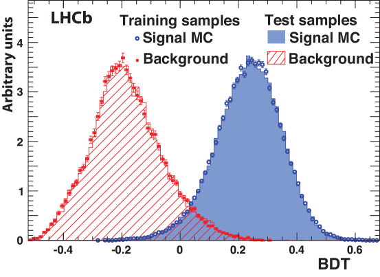
Figure 1: Distributions of the BDT variable for both training and test samples of ${J\mskip-3.0mu/\mskip-2.0mu\psi\mskip 2.0mu}\pi\pi$ signal and background events. The signal samples are from simulation and the background samples derived from data.

The ${J\mskip-3.0mu/\mskip-2.0mu\psi\mskip 2.0mu}\pi^{+}\pi^{-}$ mass distribution is shown in Fig. 2 for the $f_{\rm odd}$ region. In the $\kern 1.79993pt\overline{\kern-1.79993ptB}{}^{0}_{s}$ signal region, defined as $\pm$20 MeV around the $\kern 1.79993pt\overline{\kern-1.79993ptB}{}^{0}_{s}$ mass peak, there are 7421$\pm$105 signal events, 1717$\pm$38 combinatorial background events, and 66$\pm$9 $\eta^{\prime}$ background events, corresponding to an 81% signal purity. The $\pi^{+}\pi^{-}$ mass distribution is shown in Fig. 3. The most prominent feature is the $f_{0}(980)$, containing 52% of the events within $\pm$90 MeV of 980 MeV, called the $f_{0}$ region. The rest of the $f_{\rm odd}$ region is denoted as $\tilde{f}_{0}$.

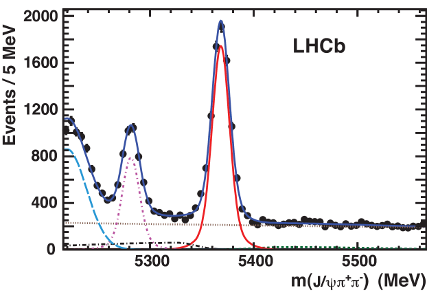
Figure 2: Mass distribution of the selected ${J\mskip-3.0mu/\mskip-2.0mu\psi\mskip 2.0mu}\pi^{+}\pi^{-}$ combinations in the $f_{\rm odd}$ region. The blue solid curve shows the result of a fit with a double Gaussian signal (red solid curve) and several background components: combinatorial background (brown dotted line), background from $B^{-}\rightarrow{J\mskip-3.0mu/\mskip-2.0mu\psi\mskip 2.0mu}K^{-}$ and ${J\mskip-3.0mu/\mskip-2.0mu\psi\mskip 2.0mu}\pi^{-}$ (green short-dashed line), $\kern 1.79993pt\overline{\kern-1.79993ptB}{}^{0}\rightarrow{J\mskip-3.0mu/\mskip-2.0mu\psi\mskip 2.0mu}\pi^{+}\pi^{-}$ (purple dot-dashed), $\kern 1.79993pt\overline{\kern-1.79993ptB}{}^{0}_{s}\rightarrow{J\mskip-3.0mu/\mskip-2.0mu\psi\mskip 2.0mu}\eta^{\prime}$ and $\kern 1.79993pt\overline{\kern-1.79993ptB}{}^{0}_{s}\rightarrow{J\mskip-3.0mu/\mskip-2.0mu\psi\mskip 2.0mu}\phi$ when $\phi\rightarrow\pi^{+}\pi^{-}\pi^{0}$ (black dot-long-dashed), and $\kern 1.79993pt\overline{\kern-1.79993ptB}{}^{0}\rightarrow{J\mskip-3.0mu/\mskip-2.0mu\psi\mskip 2.0mu}K^{-}\pi^{+}$ (light-blue long-dashed).

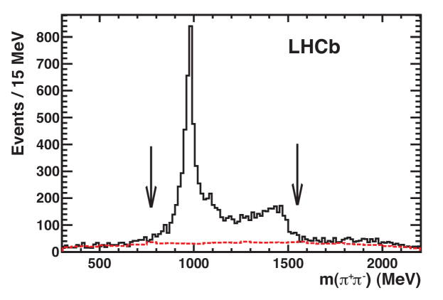
Figure 3: Mass distribution of selected $\pi^{+}\pi^{-}$ combinations shown as the (solid black) histogram for events in the $\kern 1.79993pt\overline{\kern-1.79993ptB}{}^{0}_{s}$ signal region. The (dashed red) line shows the background determined by fitting the ${J\mskip-3.0mu/\mskip-2.0mu\psi\mskip 2.0mu}\pi^{+}\pi^{-}$ mass in bins of $\pi^{+}\pi^{-}$ mass. The arrows designate the limits of the $f_{\rm odd}$ region.

3 Resonance structure in the ${J\mskip-3.0mu/\mskip-2.0mu\psi\mskip 2.0mu}\pi^{+}\pi^{-}$ final state

The resonance structure in $\kern 1.79993pt\overline{\kern-1.79993ptB}{}^{0}_{s}\rightarrow{J\mskip-3.0mu/\mskip-2.0mu\psi\mskip 2.0mu}\pi^{+}\pi^{-}$ decays has been studied using a modified Dalitz plot analysis including the decay angular distribution of the ${J\mskip-3.0mu/\mskip-2.0mu\psi\mskip 2.0mu}$ meson [11]. A fit is performed to the decay distributions of several $\pi^{+}\pi^{-}$ resonant states described by interfering decay amplitudes. The largest component is the $f_{0}(980)$ that is described by a Flatté function [22]. The data are best described by adding Breit-Wigner amplitudes for the $f_{0}(1370)$ and $f_{2}(1270)$ resonances and a non-resonant amplitude. The components and fractions of the best fit are given in Table 1.

Table 1: Resonance fractions in $\kern 1.79993pt\overline{\kern-1.79993ptB}{}^{0}_{s}\rightarrow{J\mskip-3.0mu/\mskip-2.0mu\psi\mskip 2.0mu}\pi^{+}\pi^{-}$ over the full mass range [11]. The final-state helicity of the D-wave is denoted by $\Lambda$. Only statistical uncertainties are quoted.

Resonance	Normalized fraction (%)
$f_{0}(980)$	$69.7\pm 2.3$
$f_{0}(1370)$	$21.2\pm 2.7$
non-resonant $\pi^{+}\pi^{-}$	$8.4\pm 1.5$
$f_{2}(1270)$, $\Lambda=0$	$0.49\pm 0.16$
$f_{2}(1270)$, $|\Lambda|=1$	$0.21\pm 0.65$

The final state is dominated by $C\!P$-odd S-wave over the entire $f_{\rm odd}$ region. We also have a small D-wave component associated with the $f_{2}(1270)$ resonance. Its zero helicity ($\Lambda=0$) part is also pure $C\!P$-odd and corresponds to $(0.49\pm 0.16^{+0.02}_{-0.08})\%$ of the total rate. The $|\Lambda|=1$ part, which is of mixed $C\!P$, corresponds to $(0.21\pm 0.65^{+0.01}_{-0.03})$% of the total. Performing a separate fit, we find that a possible $\rho$ contribution is smaller than 1.5% at 95% confidence level (CL). Summing the $f_{2}(1270)$ $|\Lambda|=1$ and $\rho$ rates, we find that the $C\!P$-odd fraction is larger than 0.977 at 95% CL. Thus the entire mass range can be used to study $C\!P$ violation in this almost pure $C\!P$-odd final state.

4 Flavour tagging

Knowledge of the initial $\kern 1.79993pt\overline{\kern-1.79993ptB}{}^{0}_{s}$ flavour is necessary in order to use Eq. 1. This is realized by tagging the flavour of the other $b$ hadron in the event, exploiting information from four sources: the charges of muons, electrons, kaons with significant IP, and inclusively reconstructed secondary vertices. The decisions of the four tagging algorithms are individually calibrated using $B^{\mp}\rightarrow{J\mskip-3.0mu/\mskip-2.0mu\psi\mskip 2.0mu}K^{\mp}$ decays and combined using a neural network as described in Ref. [23]. The tagging performance is characterized by $\varepsilon_{\rm tag}D^{2}$, where $\varepsilon_{\rm tag}$ is the efficiency and $D$ the dilution, defined as $D\equiv(1-2\omega)$, where $\omega$ is the probability of an incorrect tagging decision.

We use both the information of the tag decision and of the predicted per-event mistag probability. The calibration procedure assumes a linear dependence between the predicted mistag probability $\eta_{i}$ for each event and the actual mistag probability $\omega_{i}$ given by $\omega_{i}=p_{0}+p_{1}\cdot\left(\eta_{i}-\langle\eta\rangle\right)$, where $p_{0}$ and $p_{1}$ are calibration parameters and $\langle\eta\rangle$ the average estimated mistag probability as determined from the ${J\mskip-3.0mu/\mskip-2.0mu\psi\mskip 2.0mu}K^{\mp}$ calibration sample. The values are $p_{0}=0.392\pm 0.002\pm 0.009$, $p_{1}=1.035\pm 0.021\pm 0.012$, and $\langle\eta\rangle=0.391$. Systematic uncertainties are evaluated by using ${J\mskip-3.0mu/\mskip-2.0mu\psi\mskip 2.0mu}K^{+}$ separately from ${J\mskip-3.0mu/\mskip-2.0mu\psi\mskip 2.0mu}K^{-}$, performing the calibration with $\kern 1.79993pt\overline{\kern-1.79993ptB}{}^{0}\rightarrow{J\mskip-3.0mu/\mskip-2.0mu\psi\mskip 2.0mu}\kern 1.99997pt\overline{\kern-1.99997ptK}{}^{*0}$ and $\kern 1.79993pt\overline{\kern-1.79993ptB}{}^{0}\rightarrow D^{*+}\mu^{-}\overline{\nu}_{\mu}$ plus charge-conjugate channels, and viewing the dependence on different data taking periods. We find $\varepsilon_{\rm tag}=(32.9\pm 0.6)$% providing us with 2445 tagged signal events. The dilution is measured as $D=0.272\pm 0.004\pm 0.015$, leading to $\varepsilon_{\rm tag}D^{2}=(2.43\pm 0.08\pm 0.26)$%.

5 Decay time resolution

The $\kern 1.79993pt\overline{\kern-1.79993ptB}{}^{0}_{s}$ decay time is defined here as $t=m{\vec{d}\cdot\vec{p}}/{|p|^{2}}$, where $m$ is the reconstructed invariant mass, $\vec{p}$ the momentum and $\vec{d}$ the vector from the primary to the secondary vertex. The time resolution for signal increases by about 20% for decay times from 0 to 10 ps, according to both the simulation and the estimate of the resolution from the reconstruction. To take this dependence into account, we use a double-Gaussian resolution function with widths proportional to the event-by-event estimated resolution,

$$T(t-\hat{t};\sigma_{t})=\sum_{i=1}^{2}f^{T}_{i}\frac{1}{\sqrt{2\pi}S_{i}\sigma_{t}}e^{-\frac{(t-\hat{t}-\mu_{t})^{2}}{2(S_{i}\sigma_{t})^{2}}}\,,$$ (3)

where $\hat{t}$ is the true time, $\sigma_{t}$ the estimated time resolution, $\mu_{t}$ is the bias on the time measurement, $f^{T}_{1}+f^{T}_{2}=1$ are the fractions of each Gaussian, and $S_{1}$ and $S_{2}$ are scale factors.

To determine the parameters of $T$ we use events containing a ${J\mskip-3.0mu/\mskip-2.0mu\psi\mskip 2.0mu}$, found using a dimuon trigger without track impact parameter requirements, plus two opposite-sign charged tracks with similar selection criteria as for ${J\mskip-3.0mu/\mskip-2.0mu\psi\mskip 2.0mu}\pi^{+}\pi^{-}$ events including that the ${J\mskip-3.0mu/\mskip-2.0mu\psi\mskip 2.0mu}\pi^{+}\pi^{-}$ mass be within $\pm$20 MeV of the $\kern 1.79993pt\overline{\kern-1.79993ptB}{}^{0}_{s}$ mass. Figure 4 shows the decay time distribution for this ${J\mskip-3.0mu/\mskip-2.0mu\psi\mskip 2.0mu}\pi^{+}\pi^{-}$ prompt data sample for the $f_{0}$ region; the $\tilde{f}_{0}$ data are very similar. The data are fitted with the time dependence given by

$$P^{\rm prompt}(t)=(1-f_{1}-f_{2})T(t;\sigma_{t})+\left[\frac{f_{1}}{\tau_{1}}e^{{-\hat{t}}/{\tau_{1}}}+\frac{f_{2}}{\tau_{2}}e^{{-\hat{t}}/{\tau_{2}}}\right]\otimes T(t-\hat{t};\sigma_{t})\,,$$ (4)

where $f_{1}$ and $f_{2}$ are long-lived background fractions with lifetimes $\tau_{1}$ and $\tau_{2}$, respectively.

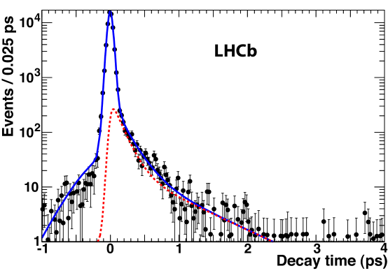
Figure 4: Decay time distribution of prompt ${J\mskip-3.0mu/\mskip-2.0mu\psi\mskip 2.0mu}\pi^{+}\pi^{-}$ candidates in the $f_{0}$ region. The dashed (red) line shows the long-lived component, and the solid curve the total.

The resulting parameter values of the function $T$ are given in Table 2.

Table 2: Parameters of the decay time resolution function determined from fits to ${J\mskip-3.0mu/\mskip-2.0mu\psi\mskip 2.0mu}\pi^{+}\pi^{-}$ prompt data samples.

Parameter	$f_{0}$ region	$\tilde{f}_{0}^{\Large\vphantom{X}}$ region
$\mu_{t}$ (fs)	$-$3.32(12)	$-$2.91(7)
$S_{1}$	1.362(4)	1.329(2)
$S_{2}$	12.969(3)	9.108(3)
$f^{T}_{2}$	0.0193(7)	0.0226(5)

Figure 5 shows the $\sigma_{t}$ distributions used in Eq. 3 for ${J\mskip-3.0mu/\mskip-2.0mu\psi\mskip 2.0mu}\pi^{+}\pi^{-}$ events in the $f_{\rm odd}$ region after background subtraction, and for like-sign background. Taking into account the calibration parameters of Table 2, the average effective decay time resolution for the signal is 40.2 fs and 39.3 fs for the $f_{0}$ and $\tilde{f}_{0}$ regions, respectively. The average of the two samples is 39.8 fs.

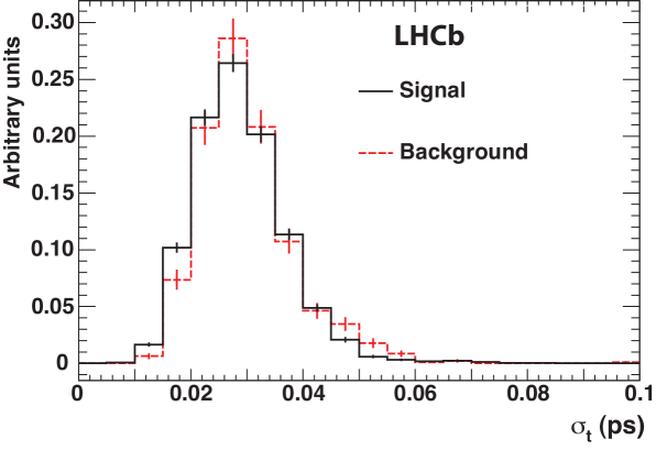
Figure 5: Distribution of the estimated time resolution $\sigma_{t}$ for opposite-sign ${J\mskip-3.0mu/\mskip-2.0mu\psi\mskip 2.0mu}\pi^{+}\pi^{-}$ signal events after background subtraction, and for like-sign background.

6 Decay time acceptance

The decay time acceptance function is written as

$$A(t;a,n,t_{0})=C\frac{\left[a\left(t-t_{0}\right)\right]^{n}}{1+\left[a\left(t-t_{0}\right)\right]^{n}}\,,$$ (5)

where $C$ is a normalization constant. The other parameters are determined by fitting the lifetime distribution of $\kern 1.79993pt\overline{\kern-1.79993ptB}{}^{0}\rightarrow{J\mskip-3.0mu/\mskip-2.0mu\psi\mskip 2.0mu}\kern 1.99997pt\overline{\kern-1.99997ptK}{}^{*0}$ events, where $\kern 1.99997pt\overline{\kern-1.99997ptK}{}^{*0}\rightarrow K^{-}\pi^{+}$. Figure 6(a) shows the ${J\mskip-3.0mu/\mskip-2.0mu\psi\mskip 2.0mu}$ $\kern 1.99997pt\overline{\kern-1.99997ptK}{}^{*0}$ mass when the $K^{-}\pi^{+}$ invariant mass is within $\pm$300 MeV of 892 MeV. There are 155,743$\pm$434 signal events. The sideband-subtracted decay time distribution is shown in Fig. 6(b) together with a lifetime fit taking into account the acceptance and resolution. This fit yields $a=2.11\pm 0.04$ ps^-1, $n=1.82\pm 0.06$, $t_{0}=0.105\pm 0.006$ ps and a lifetime of 1.516$\pm$0.008 ps, in good agreement with the PDG average of 1.519$\pm$0.007 ps [18].

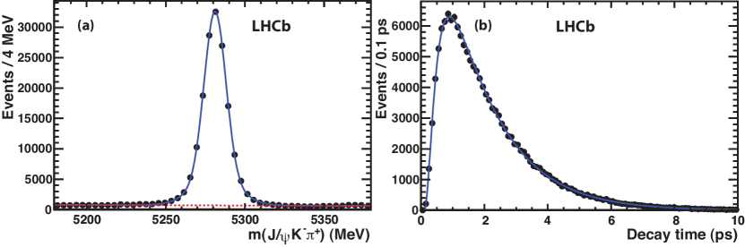
Figure 6: (a) Mass distribution of $\kern 1.79993pt\overline{\kern-1.79993ptB}{}^{0}\rightarrow{J\mskip-3.0mu/\mskip-2.0mu\psi\mskip 2.0mu}\kern 1.99997pt\overline{\kern-1.99997ptK}{}^{*0}$ candidates. The dashed (red) line shows the background, and the solid (blue) curve the total. (b) Decay time distribution, where the small background has been subtracted using the $\kern 1.79993pt\overline{\kern-1.79993ptB}{}^{0}$ mass sidebands. The (blue) curve shows the lifetime fit.

We check our lifetime acceptance by comparing with a CDF measurement of the $\kern 1.79993pt\overline{\kern-1.79993ptB}{}^{0}_{s}\rightarrow{J\mskip-3.0mu/\mskip-2.0mu\psi\mskip 2.0mu}f_{0}$ effective lifetime of $\tau^{\rm eff}=1.70^{+0.12}_{-0.11}\pm 0.03$ ps [6] obtained from a single exponential fit. A fit of the $f_{0}$ sample (see Fig. 7) yields $\tau^{\rm eff}=1.71\pm 0.03$ ps, while we find $\tau^{\rm eff}=1.67\pm 0.03$ ps in the $\tilde{f}_{0}$ sample. These two values are consistent with each other, within the quoted statistical errors, and with the CDF result.

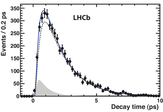
Figure 7: Decay time distribution of $\kern 1.79993pt\overline{\kern-1.79993ptB}{}^{0}_{s}\rightarrow{J\mskip-3.0mu/\mskip-2.0mu\psi\mskip 2.0mu}f_{0}$ candidates fitted with a single exponential function multiplied by the acceptance and convolved with the resolution. The dashed line is signal and the shaded area background.

7 Likelihood function definition

To determine $\phi_{s}$ an extended likelihood function is maximized using candidates in the $\kern 1.79993pt\overline{\kern-1.79993ptB}{}^{0}_{s}$ signal region

$${\cal L}(\phi_{s})=e^{-(N_{\rm sig}+N_{\rm bkg})}\prod_{i=1}^{N_{\rm obs}}P(m_{i},t_{i},{\sigma_{t}}_{i},q_{i},\eta_{i})\,,$$ (6)

where the signal yield, $N_{\rm sig}$, and background yield, $N_{\rm bkg}$, are fixed from the fit of the ${J\mskip-3.0mu/\mskip-2.0mu\psi\mskip 2.0mu}\pi^{+}\pi^{-}$ mass distribution in the $f_{\rm odd}$ region (see Fig. 2). $N_{\rm obs}$ is the number of $\kern 1.79993pt\overline{\kern-1.79993ptB}{}^{0}_{s}$ candidates, $m_{i}$ the reconstructed mass, $t_{i}$ the reconstructed decay time, and ${\sigma_{t}}_{i}$ the estimated decay time uncertainty. The flavour tag, $q_{i}$, takes values of +1, $-1$ or 0, respectively, if the signal meson is tagged as $B_{s}^{0}$, $\kern 1.79993pt\overline{\kern-1.79993ptB}{}^{0}_{s}$, or untagged, and $\eta_{i}$ is the estimated mistag probability. Backgrounds are caused largely by mis-reconstructed $b$-hadron decays, so it is necessary to include a long-lived background probability density function (PDF). The likelihood function includes distinct contributions from the signal and the background. For tagged events we have

$$P(m_{i},t_{i},{\sigma_{t}}_{i},q_{i},\eta_{i}) = N_{\rm sig}\varepsilon_{\rm tag}P_{m}^{\rm sig}(m_{i})P_{t}^{\rm sig}(t_{i},q_{i},\eta_{i}|{\sigma_{t}}_{i})P_{\sigma_{t}}^{\rm sig}({\sigma_{t}}_{i})$$ (7)

$$+N_{\rm bkg}\varepsilon^{\rm bkg}_{\rm tag}P_{m}^{\rm bkg}(m_{i})P_{t}^{\rm bkg}(t_{i}|{\sigma_{t}}_{i})P_{\sigma_{t}}^{\rm bkg}({\sigma_{t}}_{i})\,,$$

where $\varepsilon^{\rm bkg}_{\rm tag}$ refers to the flavour tagging efficiency of the background. The signal mass PDF, $P_{m}^{\rm sig}(m)$, is a double Gaussian function, while the background mass PDF, $P_{m}^{\rm bkg}(m)$, is proportional to $e^{-\alpha m}$ together with a very small contribution from $\kern 1.79993pt\overline{\kern-1.79993ptB}{}^{0}_{s}\rightarrow{J\mskip-3.0mu/\mskip-2.0mu\psi\mskip 2.0mu}\eta^{\prime}$, $N_{\eta^{\prime}}$, that is fixed in the $\phi_{s}$ fit to 66 events obtained from the fit shown in Fig. 2.

The PDF used to describe the signal decay rate, $P_{t}^{\rm sig}$, depends on the tagging results $q$ and $\eta$. It is modelled by a PDF of the true time $\hat{t}$, $R(\hat{t},q,\eta)$, convolved with the decay time resolution and multiplied by the decay time acceptance function found for $\kern 1.79993pt\overline{\kern-1.79993ptB}{}^{0}\rightarrow{J\mskip-3.0mu/\mskip-2.0mu\psi\mskip 2.0mu}\kern 1.99997pt\overline{\kern-1.99997ptK}{}^{*0}$ events. From Eq. 1, it can be expressed as

$$R(\hat{t},q,\eta)\propto e^{-\Gamma_{s}\hat{t}}\left\{\cosh\frac{\Delta\Gamma_{s}\hat{t}}{2}+\cos\phi_{s}\sinh\frac{\Delta\Gamma_{s}\hat{t}}{2}-q[1-2\omega(\eta)]\sin\phi_{s}\sin(\Delta m_{s}\hat{t})\right\}\,,$$ (8)

where $\omega(\eta)$ is the calibrated mistag probability. Thus the PDF of reconstructed time is

$$P_{t}^{\rm sig}(t,q,\eta|{\sigma_{t}})=R(\hat{t},q,\eta)\otimes T(t-\hat{t};\sigma_{t})\cdot A(t;a,n,t_{0})\,.$$ (9)

For untagged events we use

$$P(m_{i},t_{i},{\sigma_{t}}_{i},q_{i}=0,\eta_{i}) = N_{\rm sig}(1-\varepsilon_{\rm tag})P_{m}^{\rm sig}(m_{i})P_{t}^{\rm sig}(t_{i},0,\eta_{i}|{\sigma_{t}}_{i})P_{\sigma_{t}}^{\rm sig}({\sigma_{t}}_{i})$$ (10)

$$+N_{\rm bkg}(1-\varepsilon^{\rm bkg}_{\rm tag})P_{m}^{\rm bkg}(m_{i})P_{t}^{\rm bkg}(t_{i}|{\sigma_{t}}_{i})P_{\sigma_{t}}^{\rm bkg}({\sigma_{t}}_{i})\,.$$

The PDF describing the long-lived background decay rate is

$$P^{\rm bkg}_{t}(t|\sigma_{t})=\left[\frac{1-f^{\rm bkg}_{2}}{\tau^{\rm bkg}_{1}}e^{-\frac{\hat{t}}{\tau^{\rm bkg}_{1}}}+\frac{f^{\rm bkg}_{2}}{\tau^{\rm bkg}_{2}}e^{-\frac{\hat{t}}{\tau^{\rm bkg}_{2}}}\right]\otimes T(t-\hat{t};\sigma_{t})\cdot A(t;a^{\rm bkg},n^{\rm bkg},t_{0}^{\rm bkg})\,,$$ (11)

where $\tau^{\rm bkg}_{1}$, $\tau^{\rm bkg}_{2}$ and $f^{\rm bkg}_{2}$ parameterize the underlying double exponential function. The same functional form is used to describe the background decay time acceptance as for signal (Eq. 5) with different parameters that are determined by fitting the like-sign ${J\mskip-3.0mu/\mskip-2.0mu\psi\mskip 2.0mu}\pi^{\pm}\pi^{\pm}$ events in an interval $\pm$200 MeV around the $\kern 1.79993pt\overline{\kern-1.79993ptB}{}^{0}_{s}$ mass. The $P^{\rm sig}_{\sigma_{t}}({\sigma_{t}}_{i})$ and $P^{\rm bkg}_{\sigma_{t}}({\sigma_{t}}_{i})$ functions are shown in Fig. 5. The parameters that are fixed in the likelihood fit are listed in Table 3.

Table 3: Parameters used in the functions for the invariant mass and decay time describing the signal and background. These parameters are fixed to their central values in the fit for $\phi_{s}$.

Function	Parameters
	$N_{\rm sig}=7421$, $N_{\rm bkg}=1717\pm 38$, $N_{\eta^{\prime}}=66\pm 9$
$P_{m}^{\rm sig}(m)$	$m_{0}$= 5368.2(1) MeV, $\sigma^{m}_{1}$=8.1(1) MeV, $\sigma^{m}_{2}$=18.0(2) MeV, $f^{m}_{2}$= 0.196(2)
$P_{m}^{\rm bkg}(m)$	$\alpha=(-5.35\pm 1.15)\times 10^{-4}$ MeV-1
$P^{\rm bkg}_{t}(t|\sigma_{t})$	$\tau^{\rm bkg}_{1}=0.65(5)$ ps, $\tau^{\rm bkg}_{2}=2.0(8)$ ps, $f^{\rm bkg}_{2}=0.06(2)$
	$a^{\rm bkg}=3.22(10)$ ps-1, $n^{\rm bkg}=3.31(14)$, $t_{0}^{\rm bkg}=0$ ps,
$T(t-\hat{t};\sigma_{t})$	see Table 2

8 Results

The likelihood of Eq. 6 is multiplied by Gaussian constraints on several of the model parameters. These are the LHCb measured value of $\Delta m_{s}=17.63\pm 0.11\pm 0.02$ ps^-1 [24], the tagging parameters $p_{0}$ and $p_{1}$, the decay time acceptance parameters $t_{0}$, $a$, and $n$, and both $\Gamma_{s}=0.657\pm 0.009\pm 0.008$ ps^-1 and $\Delta\Gamma_{s}=0.123\pm 0.029\pm 0.011$ ps^-1 given by the ${J\mskip-3.0mu/\mskip-2.0mu\psi\mskip 2.0mu}\phi$ analysis [8]. The fit has been validated with full Monte Carlo simulations.

Figure 8 shows the difference of log-likelihood value, $\Delta\ln(\cal{L})$, compared to the one at the point with the best fit, as a function of $\phi_{s}$. At each value, the likelihood function is maximized with respect to all other parameters. The best fit value is $\phi_{s}=-0.019^{+0.173+0.004}_{-0.174-0.003}$ rad. (The systematic uncertainty will be discussed subsequently.) Values for $\phi_{s}$ in the $f_{0}$ and $\tilde{f}_{0}$ regions are $-0.26\pm 0.23$ rad and $0.29\pm 0.28$ rad, respectively, consistent within the uncertainties. The decay time distribution is shown in Fig. 9.

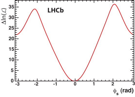
Figure 8: Log-likelihood difference as a function of $\phi_{s}$ for $\kern 1.79993pt\overline{\kern-1.79993ptB}{}^{0}_{s}\rightarrow{J\mskip-3.0mu/\mskip-2.0mu\psi\mskip 2.0mu}f_{\rm odd}$ events.

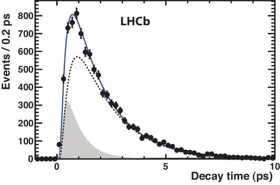
Figure 9: Decay time distribution of $\kern 1.79993pt\overline{\kern-1.79993ptB}{}^{0}_{s}\rightarrow{J\mskip-3.0mu/\mskip-2.0mu\psi\mskip 2.0mu}f_{\rm odd}$ candidates. The solid line shows the result of the fit, the dashed line shows the signal, and the shaded region the background.

The presence of a $\sin\phi_{s}$ contribution in Eq. 1 can, in principle, be viewed by plotting the asymmetry $\left[N(\kern 1.79993pt\overline{\kern-1.79993ptB}{}^{0}_{s})-N(B^{0}_{s})\right]/\left[N(\kern 1.79993pt\overline{\kern-1.79993ptB}{}^{0}_{s})+N(B^{0}_{s})\right]$ of the background-subtracted tagged yields as a function of decay time modulo $2\pi/\Delta m_{s}$, as shown in Fig. 10. The asymmetry is consistent with the value of $\phi_{s}$ determined from the full fit and does not show any significant structure.

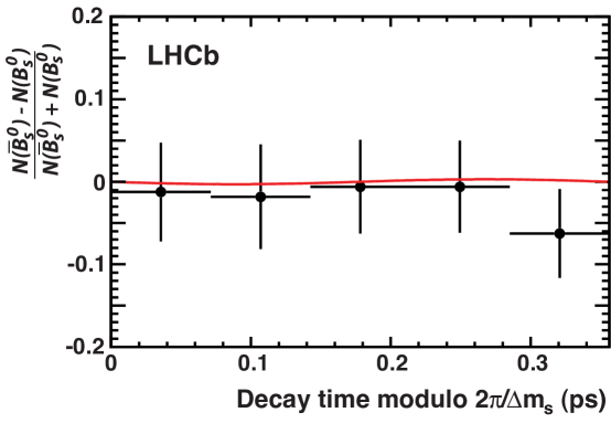
Figure 10: $C\!P$ asymmetry as a function of decay time modulo $2\pi/\Delta m_{s}$. The curve shows the expectation for $\phi_{s}=-0.019$  rad.

The data have also been analyzed allowing for the possibility of direct $C\!P$ violation. In this case Eq. 8 must be replaced with

$$R(\hat{t},q,\eta) \propto e^{-\Gamma_{s}\hat{t}}\left\{\cosh\frac{\Delta\Gamma_{s}\hat{t}}{2}+\frac{2|\lambda|}{1+|\lambda|^{2}}\cos\phi_{s}\sinh\frac{\Delta\Gamma_{s}\hat{t}}{2}\right.$$ (12)

$$\left.-\frac{q[1-2\omega(\eta)]}{1+|\lambda|^{2}}\left[2|\lambda|\sin\phi_{s}\sin(\Delta m_{s}\hat{t})-(1-|\lambda|^{2})\cos(\Delta m_{s}\hat{t})\right]\right\}\,.$$

The fit gives $|\lambda|=0.89\pm 0.13$, consistent with no direct $C\!P$ violation ($|\lambda|=1$). The value of $\phi_{s}$ changes only by $-0.002$  rad, and the uncertainty stays the same.

The systematic uncertainties are small compared to the statistical one. No additional uncertainty is introduced by the acceptance parameters, $\Delta m_{s}$, $\Gamma_{s}$, $\Delta\Gamma_{s}$ or flavour tagging, since Gaussian constraints are applied in the fit. The uncertainties associated with the fixed parameters are evaluated by changing them by $\pm$1 standard deviation from their nominal values and determining the change in the fitted value of $\phi_{s}$. These are listed in Table 4. The uncertainty due to a change in the signal time acceptance function is evaluated by multiplying $A(t;a,n,t_{0})$ with a factor $(1+\beta t)$, and redoing the $\kern 1.79993pt\overline{\kern-1.79993ptB}{}^{0}\rightarrow{J\mskip-3.0mu/\mskip-2.0mu\psi\mskip 2.0mu}\kern 1.99997pt\overline{\kern-1.99997ptK}{}^{*0}$ fit with the $\kern 1.79993pt\overline{\kern-1.79993ptB}{}^{0}$ lifetime fixed to the PDG value. The resulting value of $\beta=(1\pm 3\pm 3)\times 10^{-3}$ is then varied by $\pm 4.4\times 10^{-3}$ to estimate the uncertainty in $\phi_{s}$. An additional uncertainty is included due to a possible $C\!P$-even component. This has been limited to 2.3% of the total $f_{\rm odd}$ rate at 95% CL, and contributes an uncertainty to $\phi_{s}$ as determined by repeating the fit with an additional multiplicative dilution of 0.954. The asymmetry between $B^{0}_{s}$ and $\kern 1.79993pt\overline{\kern-1.79993ptB}{}^{0}_{s}$ production is believed to be small, and similar to the asymmetry between $B^{0}$ and $\kern 1.79993pt\overline{\kern-1.79993ptB}{}^{0}$ production which has been measured by LHCb to be about 1% [25]. The effect of neglecting this production asymmetry is the same as making a relative 1% change in the tagging efficiencies, up for $B^{0}_{s}$ and down for $\kern 1.79993pt\overline{\kern-1.79993ptB}{}^{0}_{s}$, which has a negligible effect on $\phi_{s}$.

Table 4: Summary of systematic uncertainties on $\phi_{s}$. Quantities fixed in the fit that are not included here give negligible uncertainties. The total uncertainty is found by adding in quadrature all the positive and negative contributions separately.

Quantity (Q)	$\pm\Delta$Q	$+$Change	$-$Change
		in $\phi_{s}$ (rad)	in $\phi_{s}$ (rad)
$\beta$	$4.4\times 10^{-3}$	0.0008	$-0.0007$
$\tau^{\rm bkg}_{1}$ (ps)	0.046	$-0.0006$	0.0014
$\tau^{\rm bkg}_{2}$ (ps)	0.8	$-0.0014$	0.0014
$f^{\rm bkg}_{2}$	0.02	$-0.0006$	0.0012
$N_{\rm bkg}$	38	0.0009	$-0.0001$
$N_{\eta^{\prime}}$	9	0.0006	0.0001
$m_{0}$ (MeV)	0.12	0.0012	$-0.0004$
$\sigma^{m}_{1}$ (MeV)	0.1	$-0.0002$	0.0008
$\alpha$	$1.1\times 10^{-4}$	$0.0003$	$0.0003$
$T$ function	5%	$0.0005$	0.0005
$C\!P$-even	multiply dilution by 0.954	$-0.0008$	$-$
Direct $C\!P$	free in fit	$-0.0020$	$-$
Total systematic uncertainty on $\phi_{s}$		${}^{+0.004}_{-0.003}$

9 Conclusions

Using 1 fb^-1 of data collected with the LHCb detector, $\kern 1.79993pt\overline{\kern-1.79993ptB}{}^{0}_{s}\rightarrow{J\mskip-3.0mu/\mskip-2.0mu\psi\mskip 2.0mu}\pi^{+}\pi^{-}$ decays are selected and used to measure the $C\!P$ violating phase $\phi_{s}$. The signal events have an effective decay time resolution of 39.8 fs. The flavour tagging is based on properties of the decay of the other $b$ hadron in the event and has an efficiency times dilution-squared of 2.4%. We perform a fit of the time dependent rates with the $\kern 1.79993pt\overline{\kern-1.79993ptB}{}^{0}_{s}$ lifetime and the difference in widths of the heavy and light eigenstates used as input. We measure a value of $\phi_{s}=-0.019^{+0.173+0.004}_{-0.174-0.003}$ rad. This result subsumes our previous measurement obtained with 0.41 $\mbox{\,fb}^{-1}$ of data [7]. Combining this result with our previous result from $\kern 1.79993pt\overline{\kern-1.79993ptB}{}^{0}_{s}\rightarrow{J\mskip-3.0mu/\mskip-2.0mu\psi\mskip 2.0mu}\phi$ decays [8] by performing a joint fit to the data gives a combined LHCb value of $\phi_{s}=+0.06\pm 0.12\pm 0.06$ rad. Our result is consistent with the SM prediction of $-0.0363^{+0.0016}_{-0.0015}$ rad [1]. In addition, we find no evidence for direct $C\!P$ violation.

References

- [1] CKMfitter group, J. Charles et al., Predictions of selected flavour observables within the Standard Model, Phys. Rev. D84 (2011) 033005, arXiv:1106.4041
- [2] S. Stone and L. Zhang, S-waves and the measurement of violating phases in decays, Phys. Rev. D79 (2009) 074024, arXiv:0812.2832
- [3] LHCb collaboration, R. Aaij et al., First observation of decays, Phys. Lett. B698 (2011) 115, arXiv:1102.0206
- [4] Belle collaboration, J. Li et al., Observation of and evidence for , Phys. Rev. Lett. 106 (2011) 121802, arXiv:1102.2759
- [5] D0 collaboration, V. M. Abazov et al., Measurement of the relative branching ratio of to , Phys. Rev. D85 (2012) 011103, arXiv:1110.4272
- [6] CDF collaboration, T. Aaltonen et al., Measurement of branching ratio and lifetime in the decay at CDF, Phys. Rev. D84 (2011) 052012, arXiv:1106.3682
- [7] LHCb collaboration, R. Aaij et al., Measurement of the violating phase in , Phys. Lett. B707 (2012) 497, arXiv:1112.3056
- [8] LHCb collaboration, R. Aaij et al., Measurement of the CP-violating phase in the decay , Phys. Rev. Lett. 108 (2012) 101803, arXiv:1112.3183
- [9] D0 collaboration, V. M. Abazov et al., Measurement of the CP-violating phase using the flavor-tagged decay in 8 fb-1 of collisions, Phys. Rev. D85 (2012) 032006, arXiv:1109.3166
- [10] CDF collaboration, T. Aaltonen et al., Measurement of the -violating phase in decays with the CDF II detector, arXiv:1112.1726
- [11] LHCb collaboration, R. Aaij et al., Analysis of the resonant components in , arXiv:1204.5675, Submitted to Phys. Rev. D
- [12] S. Faller, R. Fleischer, and T. Mannel, Precision physics with at the LHC: the quest for new physics, Phys. Rev. D79 (2009) 014005, arXiv:0810.4248
- [13] R. Fleischer, R. Knegjens, and G. Ricciardi, Anatomy of , Eur. Phys. J. C71 (2011) 1832, arXiv:1109.1112
- [14] U. Nierste, Three lectures on meson mixing and CKM phenomenology, arXiv:0904.1869
- [15] I. I. Bigi and A. Sanda, CP violation, Camb. Monogr. Part. Phys. Nucl. Phys. Cosmol. 9 (2000) 1
- [16] LHCb collaboration, R. Aaij et al., Determination of the sign of the decay width difference in the system, arXiv:1202.4717, submitted to Phys. Rev. Lett.
- [17] LHCb collaboration, A. Alves Jr. et al., The LHCb detector at the LHC, JINST 3 (2008) S08005
- [18] Particle Data Group, K. Nakamura et al., Review of particle physics, J. Phys. G37 (2010) 075021
- [19] A. Hoecker et al., TMVA - Toolkit for multivariate data analysis, PoS ACAT (2007) 040, arXiv:physics/0703039
- [20] T. Sjstrand, S. Mrenna, and P. Skands, PYTHIA 6.4 physics and manual, JHEP 05 (2006) 026, arXiv:hep-ph/0603175
- [21] GEANT4 collaboration, S. Agostinelli et al., GEANT4: A Simulation toolkit, Nucl. Instrum. Meth. A506 (2003) 250
- [22] S. M. Flatté, On the nature of 0+ mesons, Phys. Lett. B63 (1976) 228
- [23] LHCb collaboration, R. Aaij et al., Opposite-side flavour tagging of B mesons at the LHCb experiment, arXiv:1202.4979, submitted to Eur. Phys. J. C
- [24] LHCb collaboration, R. Aaij et al., Measurement of the oscillation frequency in the decays , Phys. Lett. B709 (2012) 177, arXiv:1112.4311
- [25] LHCb collaboration, R. Aaij et al., First evidence of direct violation in charmless two-body decays of mesons, arXiv:1202.6251