Thermoelectric probe for Rashba spin-orbit interaction strength in a two dimensional electron gas

Abstract

Thermoelectric coefficients of a two dimensional electron gas (2DEG) with the Rashba spin-orbit interaction (SOI) are presented here. In absence of magnetic field, thermoelectric coefficients are enhanced due to the Rashba SOI. In presence of magnetic field, the thermoelectric coefficients of spin-up and spin-down electrons oscillate with different frequency and produces beating patterns in the components of the total thermoelectric power and the total thermal conductivity. We also provide analytical expressions of the thermoelectric coefficients to explain the beating pattern formation. We obtain a simple relation which determines the Rashba SOI strength if the magnetic fields corresponding to any two successive beat nodes are known from the experiment.

I Introduction

There has been a rapid growth of research interest on the Rashba SOI in low-dimensional condensed matter system after the proposal of spin field effect transistor by Datta and Das das1 . This is due to the possible applications in spintronics devices appl1 ; appl2 ; appl3 . The SOI is responsible for other interesting effects like spin Hall effect she , spin dynamics and zitterbewegung zb ; spin ; zb1 . In the narrow gap semiconductor heterostructures, the dominant Rashba SOI rashba ; rashba1 appears due to the asymmetric quantum wells. The Rashba SOI strength is proportional to the internally generated crystal field. This strength can also be enhanced by applying suitable electric field perpendicular to the plane of the electron’s motion tech ; matsu .

A pseudo Zeeman effect occurs at finite momentum of the electron due to the Rashba SOI even in absence of magnetic field. A direct manifestation of pseudo Zeeman effect due to the SOI is a regular beating pattern in the magnetoelectric transport measurements such as Shubnikov-de Hass (SdH) oscillations beat_exp in 2DEG. These oscillations occur due to two closely spaced different frequency of spin-up and spin-down electrons. The Rashba SOI strength is determined by analyzing the beating patterns in the SdH oscillations miller ; datta1 . The SOI was determined by fitting the experimental data with the model calculations for the SdH oscillations. Later, many realistic approach was considered and the estimated strength is in good agreement with the extrapolated results alter1 ; alter2 ; firoz . Recently, there is an interesting proposal firoz1 of determining the Rashba SOI strength by analyzing the beating patterns in the Weiss oscillations weiss ; weiss1 .

On the other hand, thermoelectric properties of materials nolas have attracted considerable interest from both experimental and theoretical point of view due to potential applications in technology application ; application1 . There is a strong effect of perpendicular magnetic field on thermal transport properties of any system. Therefore, the magnetothermal coefficients can be used as an additional probe. In presence of perpendicular magnetic field, the diffusing charge carriers experience the Lorentz force. This produces a transverse electric field in addition to the longitudinal electric field. The longitudinal thermopower or the Seebeck coefficient is defined as $S_{xx}=-\frac{\nabla V_{x}}{\nabla T}$. On the other hand, the transverse thermopower or the Nernst coefficient is defined as $S_{xy}=-\frac{\nabla V_{x}}{\nabla T}$. Here, $\nabla V_{x}$ and $\nabla V_{y}$ are the induced voltage generated by the thermal gradient and the magnetic field, respectively. Theoretical and experimental studies on thermoelectric coefficients of 2DEG systems in presence of magnetic field started after the discovery of the quantum Hall effect. In most of the thermoelectric measurements of 2DEG systems, the thermopower is being measured since the thermal resistivity of a 2DEG is extremely high. The Nernst coefficient is quite sensitive to various properties of the systems e.g. shape of the Fermi surface as well as electron mean free path behnia . It is being used as a probe to study various strongly correlated electron systems such as Kondo lattices behnia1 and graphene field effect transistors graphene ; graphene1 . Moreover, the thermopower $S$ and the thermal conductivity $\kappa$ are used as the metrics to measure the thermoelectric performance behnia . In addition to these, we will show here that magntethermoelectric coefficients can also be used to determine the Rashba SOI strength.

There are mainly two mechanisms contribute to the thermal conductivity and the thermopower, namely the thermodiffusion and phonon drag. Generally, the phonon drag contribution is vanishingly small at very low temperature. In absence of the magnetic field, the diffusive thermopower has been continuously reported in the low range of temperature kundu ; exp1 ; syme ; rafael ; reno ; epl ; seebek . In presence of magnetic field, the oscillation of the diffusive thermopower has been studied theoretically as well as experimentally prb86 ; prb95 ; topical ; maximov ; arindam . It is seen in the low magnetic field regime that both $S_{xx}$ and $S_{xy}$ are periodic in inverse of the magnetic field. This is due to the oscillating density of states of the 2DEG in presence of magnetic field.

There is no theoretical or experimental study on magnetothermoelectric properties of the 2DEG systems with the Rashba SOI. We report here for the first time the effect of the Rashba SOI on thermal transport properties of a 2DEG in presence of perpendicular magnetic field. The total thermalconductivity and the total thermopower produce beating patterns because the thermoelectric coefficients for spin-up and spin-down electrons oscillate with two closely spaced different frequencies. By analyzing the beating pattern, we find a simple equation which determines the Rashba SOI strength if the magnetic fields corresponding to any two successive beat nodes and the number of oscillations in between are known from the experiment.

This paper is organized as follows. In section II, we briefly mention the energy spectrum and the DOS of the 2DEG with the Rashba SOI for zero and non-zero magnetic field cases. In section III, we have studied the thermoelectric coefficients for zero magnetic field case. We also provide the formalism to be used for studying thermoelectric coefficients in presence of magnetic field. In section IV, we present our numerical and analytical results. We provide a summary and conclusion of our work in section V.

II ENERGY SPECTRUM AND DENSITY OF STATES of a 2DEG with the Rashba SOI

II.1 Zero magnetic field case

The Hamiltonian of an electron with the Rashba SOI is given by rashba

$$H=\frac{{\bf p}^{2}}{2m^{\ast}}\mathbb{1}+\frac{\alpha}{\hbar}({\mbox{\boldmath$\sigma$}}\times p)_{z},$$ (1)

where ${\bf p}$ is the two-dimensional momentum operator, $m^{\ast}$ is the effective mass of the electron, $\mathbb{1}$ is the unit matrix, ${\mbox{\boldmath$\sigma$}}=(\sigma_{x},\sigma_{y},\sigma_{z})$ are the Pauli spin matrices and $\alpha$ is the strength of the Rashba SOI. At non-zero momentum, the spin degeneracy is lifted due to the presence of the SOI. The energy spectrum of the ”spin-up” and ”spin-down” electron is given by

$$E^{\pm}=\frac{\hbar^{2}k^{2}}{2m^{*}}\pm\alpha\mid k\mid.$$ (2)

Here, the + and - signs correspond to the spin-up and spin-down electrons. The density of states (DOS) winkler for spin-up and spin-down electrons are

$$g^{+}(E)=\frac{D_{0}}{2}\Big{[}1+\sqrt{\frac{E_{\alpha}}{E_{\alpha}+4E}}\Big{]}\Theta(E)$$ (3)

and

$$g^{-}(E) = \frac{D_{0}}{2}\Big{[}1-\sqrt{\frac{E_{\alpha}}{E_{\alpha}+4E}}\Big{]}\Theta(E)$$ (4)

$$+ D_{0}\sqrt{\frac{E_{\alpha}}{E_{\alpha}+4E}}\Theta(-E)\Theta(E+E_{\alpha}/4).$$

Here, $D_{0}=m^{*}/(\pi\hbar^{2})$, $E_{\alpha}=2m^{\ast}\alpha^{2}/\hbar^{2}$ is the Rashba energy determined by the Rashba SOI strength $\alpha$ and $\Theta(E)$ is the unit step function.

II.2 Non-zero magnetic field case

The Hamiltonian of an electron $(-e)$ with the Rashba SOI in presence of a perpendicular magnetic field ${\bf B}=B\hat{z}$ is given by

$$H=\frac{({\bf p}+e{\bf A})^{2}}{2m^{\ast}}\mathbb{1}+\frac{\alpha}{\hbar}\left[{\mbox{\boldmath$\sigma$}}\times({\bf p}+e{\bf A})\right]_{z}+\frac{1}{2}g\mu_{{}_{B}}B\sigma_{z},$$ (5)

where $\mu_{{}_{B}}=e\hbar/(2m_{e})$ is the Bohr magneton with $m_{e}$ is the free electron mass and $g$ is the effective Lande $g$-factor. The exact energy spectrum and the corresponding eigenfunctions of the above Hamiltonian are derived in Ref. alter1 . The resulting eigenstates are labeled by a new quantum number $s$. For $s=0$, there is only one energy level which is same as the lowest Landau level without the Rashba SOI. The corresponding energy is given by $E_{0}^{+}=E_{0}=(\hbar\omega-g\mu_{{}_{B}}B)/2$. Here, $\omega=eB/m^{*}$ is cyclotron frequency. For $s=1,2,3....$, there are two branches of the energy levels, denoted by $+$ corresponding to the ”spin-up” electrons and $-$ corresponding to the ”spin-down” electrons with energies

$$E_{s}^{\pm}=s\hbar\omega{\pm}\sqrt{E_{0}^{2}+sE_{\alpha}\hbar\omega}.$$ (6)

Using the Green’s function method, the DOS for spin-up and spin-down electrons in presence of magnetic field are calculated in Ref. firoz . These are given by

$$D^{\pm}(E) \backsimeq \frac{D_{0}}{2}\Big{[}1+2\exp{\Big{\{}-2\Big{(}\frac{\pi\Gamma_{0}}{\hbar\omega}\Big{)}^{2}\Big{\}}}$$ (7)

$$\times \cos{\Big{\{}\frac{2\pi}{\hbar\omega}\Big{(}E+\frac{E_{\alpha}}{2}\mp\sqrt{E_{0}^{2}+E_{\alpha}E}\Big{)}\Big{\}}}\Big{]},$$

where $\Gamma_{0}$ is the impurity induced Landau level broadening.

III Thermoelectric coefficients

In this section, we shall develop the formalism for the thermoelectric coefficients of a 2DEG with the Rashba SOI system for both the cases: zero and non-zero magnetic fields.

III.1 Zero magnetic field case

In this sub-section, we consider a 2DEG with the Rashba SOI and calculate the thermal power and thermal conductivity. Within the linear response regime, the electrical current density ${\bf J}$ and the thermal current density ${\bf J}_{q}$ for spin-up and spin-down electrons can be written as

$${\bf J}_{\pm}=L_{\pm}^{11}{\bf E}+L_{\pm}^{12}(-\nabla T)$$ (8)

and

$${\bf J}_{\pm}^{q}=L_{\pm}^{21}{\bf E}+L_{\pm}^{22}(-\nabla T),$$ (9)

where ${\bf E}$ is the electric field and $L_{\pm}^{ij}$ with $i,j=1,2$ are the phenomenological transport coefficients for spin-up and spin-down electrons in absence of magnetic field. These are the main equations that determine the response of a system to the external forces such as electric field and temperature gradient. In presence of the Rashba SOI, the spin-up and spin-down electrons will contribute to the total electrical and thermal current. Therefore, the total electrical current and the thermal current densities are

$${\bf J}=L^{11}{\bf E}+L^{12}(-\nabla T)$$ (10)

and

$${\bf J}^{q}=L^{21}{\bf E}+L^{22}(-\nabla T).$$ (11)

Here, $L^{ij}=L_{+}^{ij}+L_{-}^{ij}$ and $L^{ij}$ can be written in terms of the integral $I^{(r)}$: $L^{11}=I^{(0)},L^{21}=TL^{12}=-I^{(1)}/e$, $L^{22}=I^{(2)}/(e^{2}T)$. Also, $I^{(r)}=I^{(r),+}+I^{(r),-}$ with

$$I^{(r),\pm}=\int dE\Big{[}-\frac{\partial f(E)}{\partial E}\Big{]}(E-\eta)^{r}\sigma^{\pm}(E),$$ (12)

where $r=0,1,2$ and $f(E)=1/[1+exp(E-\eta)\beta]$ is the Fermi-Dirac distribution function with $\eta$ is the chemical potential and $\beta=1/(k_{{}_{B}}T)$. Here, $\sigma^{+}(E)$ and $\sigma^{-}(E)$ are the energy-dependent conductivity for spin-up and spin-down electrons, respectively. In an open circuit condition ($J=0$), the thermopower is given by $S=L^{12}/L^{11}$. Then at low temperature, diffusion thermopower $S$ and the diffusion thermal conductivity $\kappa$ can be expressed in terms of the electrical conductivity through the Mott’s relation and the Wiedemann-Franz law as

$$S=-L_{0}eT\Big{[}\frac{d}{dE}\ln\sigma(E)\Big{]}_{{}_{E=E_{F}}}$$ (13)

and

$$\kappa=L_{0}T\sigma(E_{{}_{F}}).$$ (14)

Here, $L_{0}=(\pi^{2}k_{{}_{B}}^{2})/(3e^{2})$ is the Lorentz number and $\sigma(E_{{}_{F}})=\sigma^{+}(E_{{}_{F}})+\sigma^{-}(E_{{}_{F}})$ is the total electrical conductivity at the Fermi energy.

By using the Boltzmann transport equation, we evaluate the zero-temperature energy-dependent electrical conductivity for spin-up and spin-down electrons, which are given by

$$\sigma^{\pm}(E)=\frac{e^{2}}{m^{*}}\tau(E)g^{\pm}(E)\Big{[}E+\frac{E_{\alpha}}{4}\Big{]}.$$ (15)

Assuming the energy dependent scattering time to be $\tau=\tau_{0}(E/E_{{}_{F}})^{p}$, where $p$ is a constant depending on the scattering mechanism. We also assumed that $\tau$ is the same for spin-up and spin-down electrons. Substituting Eqs. (3), (4) and (15) into Eq. (13), then the diffusion thermopower is obtained as

$$S=-L_{0}\frac{eT}{E_{F}}\Big{[}p+1-\frac{E_{\alpha}}{4E_{F}}\Big{]}.$$ (16)

We calculate the total electrical conductivity $\sigma(E_{{}_{F}})$ at the Fermi level, which is given as

$$\sigma(E_{{}_{F}})=\frac{ne^{2}\tau_{0}}{m^{*}}+\frac{m^{*}e^{2}\tau_{0}\alpha^{2}}{2\pi\hbar^{4}}=\sigma_{0}\Big{[}1+\frac{E_{\alpha}}{4E_{F}}\Big{]},$$ (17)

where $\sigma_{0}=\frac{ne^{2}\tau_{0}}{m^{*}}$ is the Drude conductivity without SOI. The similar expression of the Drude conductivity is obtained by using a different method in Ref. vasi . The total thermal conductivity is then

$$\kappa=L_{0}T\sigma_{0}\Big{(}1+\frac{E_{\alpha}}{4E_{F}}\Big{)}.$$ (18)

We note that the thermal conductivity and the thermopower is enhanced due to the presence of the Rashba SOI.

III.2 Non-zero magnetic field case

In this subsection, we shall study the thermoelectric coefficients of a 2DEG with the Rashba SOI in presence of the perpendicular magnetic field. Thermoelectric coefficients in presence of magnetic field (without SOI) were obtained by modifying the Kubo formula in Ref. streda ; oji . Here we shall generalize these results to the SOI systems. These phenomenological transport coefficients can be re-written as

$$\sigma_{\mu\nu}^{\pm}={\cal L}_{\mu\nu}^{(0),\pm}$$ (19)

$$S_{\mu\nu}^{\pm}=\frac{1}{eT}[({\cal L}^{(0),\pm})^{-1}{\cal L}^{(1),\pm}]_{\mu\nu}$$ (20)

$$\kappa_{\mu\nu}^{\pm}=\frac{1}{e^{2}T}[{\cal L}_{\mu\nu}^{(2),\pm}-eT({\cal L}^{(1),\pm}S^{\pm})_{\mu\nu}],$$ (21)

where

$${\cal L}_{\mu\nu}^{(r),\pm}=\int dE\Big{[}-\frac{\partial f(E)}{\partial E}\Big{]}(E-\eta)^{r}\sigma_{\mu\nu}^{\pm}(E).$$ (22)

Here, $\mu,\nu=x,y$. Also, $\sigma_{\mu\nu}^{\pm}(E)$, $S_{\mu\nu}^{\pm}$ and $\kappa_{\mu\nu}^{\pm}$ are the zero-temperature energy-dependent conductivity, thermopower and thermal conductivity tensors, respectively, for spin-up and spin-down electrons. The total thermopower and thermal conductivity can be obtained from $S_{\mu\nu}=S_{\mu\nu}^{+}+S_{\mu\nu}^{-}$ and $\kappa_{\mu\nu}=\kappa_{\mu\nu}^{+}+\kappa_{\mu\nu}^{-}$.

In electron systems, conduction of carriers takes place by the diffusive and collisional mechanisms. The collisional contribution leads to the SdH oscillation with inverse magnetic field due to the quantized nature of the energy spectrum. We will consider the collisional mechanism only because electrons do not possess any drift velocity in our case. In the linear response regime, the conductivity tensor can be written as the sum of diagonal and non-diagonal as $\sigma_{\mu\nu}=\sigma_{\mu\nu}^{\rm d}+\sigma_{\mu\nu}^{{\rm nd}}$, where $\sigma_{\mu\nu}^{\rm nd}$ is the Hall contribution. Here, $\sigma_{xx}=\sigma_{xx}^{\rm col}$ and $\sigma_{yy}=\sigma_{xx}^{\rm col}+\sigma_{yy}^{\rm dif}=\sigma_{xx}^{\rm col}$. Similarly, for the thermal transport coefficients the following relations are valid: ${\cal L}_{xx}^{(r)}={\cal L}_{xx}^{(r){\rm col}}={\cal L}_{yy}^{(r){\rm col}}$ and ${\cal L}_{yy}^{(r)}={\cal L}_{yy}^{(r){\rm dif}}+{\cal L}_{yy}^{(r){\rm col}}={\cal L}_{yy}^{(r){\rm col}}$. The exact form of the finite temperature collisional conductivity has been calculated in Ref. alter1 for the screened impurity potential $U({\bf q})=2\pi e^{2}/(\epsilon\sqrt{q_{x}^{2}+q_{y}^{2}+k_{s}^{2}})$ in momentum space. Here, $k_{s}$ is the inverse screening length and $\epsilon$ is the dielectric constant of the material. In the limit of small $|{\bf q}|\ll k_{s}$, $U({\bf q})\simeq 2\pi e^{2}/(\epsilon k_{s})=U_{0}$. In this limit, one can use $\tau_{0}^{2}\approx\pi l^{2}\hbar^{2}/N_{I}U_{0}^{2}$ with $\tau_{0}$ is the collisional time, $l=\sqrt{\hbar/eB}$ is the magnetic length scale, $U_{0}$ is the strength of the screened impurity potential and $N_{I}$ is the two-dimensional impurity density. The exact form of the finite temperature conductivity can be reduced to the zero-temperature energy-dependent electrical conductivity as

$$\sigma_{xx}^{\pm}(E)=\frac{e^{2}}{h}\frac{N_{I}U_{0}^{2}}{2\pi\Gamma_{0}l^{2}}I_{s}^{\pm},$$ (23)

where $I_{s}^{\pm}=[(2s\mp 1)D_{s}^{4}-2sD_{s}^{2}+(2s\pm 1)]/A_{s}^{2}$ with $D_{s}=\sqrt{sE_{\alpha}\hbar\omega}/[E_{0}+\sqrt{E_{0}^{2}+sE_{\alpha}\hbar\omega}]$ and $A_{s}=1+D_{s}^{2}$. Using Eq. (22), the finite temperature diagonal and off-diagonal coefficients (${\cal L}_{xx}^{(r)}$ and ${\cal L}_{yx}^{(r)}$) can be written as

$${\cal L}_{xx}^{(r),\pm}=\frac{e^{2}}{h}\frac{N_{I}U_{0}^{2}}{2\pi\Gamma_{0}l^{2}}\sum_{s}I_{s}^{\pm}\Big{[}(E-\eta)^{r}\Big{(}-\frac{\partial f(E)}{\partial E}\Big{)}\Big{]}_{E=E_{s}^{\pm}}$$ (24)

and

$${\cal L}_{yx}^{(r),\pm} = \frac{e^{2}}{h}\sum_{s}\frac{\Big{[}D_{s+1}(D_{s}\sqrt{s}\mp\sqrt{2}k_{\alpha}l)+\sqrt{s+1}\Big{]}^{2}}{{A_{s}A_{s+1}}}$$ (25)

$$\times \int_{E_{s}^{\pm}}^{E_{s+1}^{\pm}}dE\Big{[}(E-\eta)^{r}\Big{(}-\frac{\partial f(E)}{\partial E}\Big{)}\Big{]}_{E=E_{s}^{\pm}}.$$

IV Numerical results and discussions

In our numerical calculations, the following parameters are used: carrier concentration $n_{e}=3\times 10^{15}$ /m², effective mass $m^{*}=0.05m_{e}$ with $m_{e}$ is the free electron mass, $g=4$ and the Rashba SOI strength $\alpha=5\times 10^{-12}$ eV-m and $\Gamma_{0}=0.01$ meV. For better visualization of the oscillations, we have used $T=1$ K for the thermopower, $T=0.5$ K for the thermal conductivity. In Fig. [1], the components of the thermopower tensor in units of $-k_{{}_{B}}/e$ are shown as a function of the inverse magnetic field. The diagonal thermopower components $S_{xx}$ and $S_{yy}$ are identical and therefore only $S_{xx}$ is shown. In Fig. [2], the thermal conductivity is shown as a function of the inverse magnetic field. The magnetic field dependence of the thermal conductivity is same as that of the electrical conductivity. Figures [1] and [2] show the appearance of the beating pattern in the thermopower and thermal conductivity.

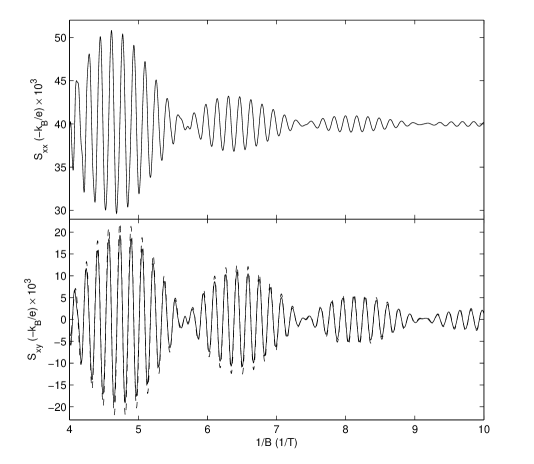
Figure 1: Plots of the thermopower versus inverse magnetic field. In the lower panel, dashed and solid lines correspond to the analytical and exact results, respectively.

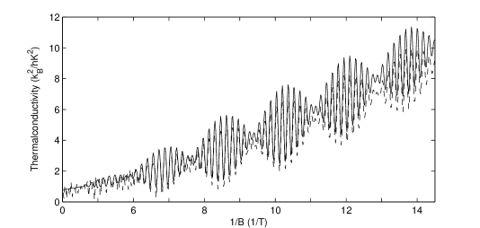
Figure 2: Plots of the longitudinal component of thermalconductiviy $\kappa_{xx}$ versus inverse magnetic field $B$. The dashed and solid lines correspond to the exact numerical and analytical results.

To analyze the beating pattern in the thermoelectric coefficients, we shall derive analytical expressions of the thermoelectric coefficients. The components of the thermopower for spin-up and spin-down electrons are given by

$$S_{xx}^{\pm}=S_{yy}^{\pm}=\frac{1}{eT}\Big{[}\frac{\sigma_{xx}^{\pm}}{S_{0}}{\cal L}_{xx}^{(1),\pm}+\frac{{\cal L}_{yx}^{(1),\pm}}{\sigma_{yx}^{\pm}}\Big{]}$$ (26)

and

$$S_{xy}^{\pm}=-S_{yx}^{\pm}=\frac{1}{eT}\Big{[}\frac{\sigma_{xx}^{\pm}}{S_{0}}(-{\cal L}_{xy}^{(1),\pm})+\frac{{\cal L}_{xx}^{(1),\pm}}{\sigma_{yx}^{\pm}}\Big{]}.$$ (27)

The dominating term in the above two equations is the last term. The analytical form of $\kappa_{xx}$ and $S_{xy}$ can be obtained directly by deriving analytical form of the phenomenological transport coefficients. The analytical form of the DOS given in Eq. (7) allows us to obtain asymptotic expressions of $S_{xy}$ and $\kappa_{xx}$. This is done by replacing the summation over discrete quantum numbers $s$ by the integration i.e; $\sum_{s}\rightarrow 2\pi l^{2}\int D^{\pm}(E)dE$, then we get

$${\cal L}_{xx}^{(1),\pm}\simeq\Big{(}\frac{-\pi}{\beta}\Big{)}\frac{\sigma_{0}}{8(\omega\tau_{0})^{2}}\Omega_{D}G^{\prime}(x)\sin\Big{(}2\pi\frac{f^{\pm}}{B}\Big{)}$$ (28)

and

$${\cal L}_{xx}^{(2),\pm}\simeq\Big{(}\frac{\pi}{\beta}\Big{)}^{2}\frac{\sigma_{0}}{8(\omega\tau_{0})^{2}}\Big{[}\frac{1}{3}-\frac{\Omega_{D}}{2}G^{\prime\prime}(x)\cos\Big{(}2\pi\frac{f^{\pm}}{B}\Big{)}\Big{]},$$ (29)

where the impurity induced damping factor is

$$\Omega_{D}=2\exp\Big{\{}-2\Big{(}\frac{\pi\Gamma_{0}}{\hbar\omega}\Big{)}^{2}\Big{\}}$$ (30)

and the temperature dependent damping factor is the derivative of the function $G(x)$ with $G(x)=x/\sinh(x)$. Here, $x=T/T_{c}$ with $T_{c}=\hbar\omega/2\pi^{2}k_{{}_{B}}$. Note that $G(x)$ is the temperature dependent damping factor for the electrical conductivity tensor. Also, the oscillation frequencies are

$$f^{\pm}=\frac{m^{*}}{\hbar e}\Big{[}E_{F}+\frac{E_{\alpha}}{2}\mp\sqrt{E_{0}^{2}+E_{\alpha}E_{F}}\Big{]}.$$ (31)

The off-diagonal thermopower $S_{xy}$ for spin-up and spin-down electron is obtained as

$$S_{xy}^{\pm}=-\frac{k_{{}_{B}}}{e}\frac{\pi}{4\omega\tau_{0}}\Omega_{D}G^{\prime}(x)\sin\Big{(}2\pi\frac{f^{\pm}}{B}\Big{)}.$$ (32)

The total thermopower is given as

$$S_{xy}=-\frac{k_{{}_{B}}}{e}\frac{\pi}{2\omega\tau_{0}}\Omega_{D}G^{\prime}(x)\sin\Big{(}2\pi\frac{f_{\rm a}}{B}\Big{)}\cos\Big{(}2\pi\frac{f_{\rm d}}{B}\Big{)}.$$ (33)

Here, $f_{\rm a}=(f^{+}+f^{-})/2$ and $f_{\rm d}=(f^{+}-f^{-})/2$. In the lower panel of Fig. [1], we compare the analytical expression of $S_{xy}$ with that of the numerical result. The analytical result matches very well with the numerical results.

For thermal conductivity, the dominant term in $\kappa_{xx}$ is ${\cal L}_{xx}^{(2)}$. The approximate analytical form of $\kappa_{xx}^{\pm}$ can be obtained from Eqs. (21) and (29) as

$$\kappa_{xx}^{\pm}\simeq L_{0}\frac{T\sigma_{0}}{8(\omega\tau_{0})^{2}}\Big{[}1-\frac{3}{2}\Omega_{D}G^{\prime\prime}(x)\cos\Big{(}2\pi\frac{f^{\pm}}{B}\Big{)}\Big{]}.$$ (34)

The total thermal conductivity can be written as

$$\kappa_{xx} \simeq L_{0}\frac{\sigma_{0}T}{4(\omega\tau_{0})^{2}}\Big{[}1-\frac{3}{2}\Omega_{D}G^{\prime\prime}(x)$$ (35)

$$\times \cos\Big{(}2\pi\frac{f_{\rm a}}{B}\Big{)}\cos\Big{(}2\pi\frac{f_{\rm d}}{B}\Big{)}\Big{]}.$$

Equations (32) and (34) show that the thermopower and the thermalconductivity of spin-up and spin-down electron oscillates with different frequency $f^{+}$ and $f^{-}$, respectively. Therefore, the beating pattern appears in the total $S_{xy}$ and $\kappa$. It is quite difficult to obtain the analytical expression of $S_{yy}$, but the origin of the oscillatory part is due to the oscillatory density of states at the Fermi energy.

We get the condition for beating nodes from the periodic term with frequency difference $f_{\rm d}$: $\cos(2\pi f_{\rm d}/B)_{B=B_{j}}=0$ which gives

$$\sqrt{\Delta_{s}^{2}+(1-g^{*})^{2}(\hbar\omega_{j})^{2}}=\hbar\omega_{j}(j+\frac{1}{2}).$$ (36)

Here, $\Delta_{s}=2k_{{}_{F}}\alpha$ is the zero-field spin splitting energy with $k_{{}_{F}}$ is the Fermi wave vector, $j=1,2,3..$ is the j-th beat node and $g^{*}=gm^{*}/(2m_{e})$. Also, $\omega_{j}=eB_{j}/m^{*}$ and $B_{j}$ is the magnetic field corresponding to the $j$-th beat node. Using the above equation, one can determine the zero-field spin splitting energy or the Rashba strength if we know the number ($j$) of any node and the corresponding magnetic field $B_{j}$. In practice, the numbering of the beat nodes is quite difficult. The above equation can be re-written for two successive beating nodes as

$$\sqrt{\Big{(}\frac{\Delta_{s}}{\hbar\omega_{j+1}}\Big{)}^{2}+(1-g^{*})^{2}}-\sqrt{\Big{(}\frac{\Delta_{s}}{\hbar\omega_{j}}\Big{)}^{2}+(1-g^{*})^{2}}=1.$$ (37)

Therefore, the Rashba SOI strength can be determined from Eq. (37) by knowing the magnetic fields correspond to any two successive beat nodes.

In the above analytical expressions [Eqs. (33) and (35)] the periodic term with frequency $f_{\rm a}$ gives the number of oscillations between the two successive beat nodes as given by

$$N_{\rm osc}=\frac{m^{*}}{e\hbar}\Big{(}E_{F}+\frac{E_{\alpha}}{2}\Big{)}\Big{(}\frac{1}{B_{j+1}}-\frac{1}{B_{j}}\Big{)}.$$ (38)

Therefore, we can also determine the Rashba strength from Eq. (38) by knowing the magnetic fields correspond to any two successive beat nodes and the number of oscillations in between. We note that Eqs. (36) and (38) are the same as obtained in the beating pattern formation in the SdH oscillations firoz .

V conclusion

We present theoretical study of the effect of the Rashba SOI on the thermoelectric coefficients. In absence of magnetic field, the thermopower and the thermal conductivity are enhanced due to the presence of the SOI. The numerical results of all the thermoelectric coefficients are given. In addition to the numerical results, we provide the analytical expressions of the off-diagonal component of the thermopower $(S_{xy})$ and the diagonal components of the thermal conductivity ($\kappa_{xx}$). The appearance of the beating pattern in the thermoelectric coefficients can be explained from the fact that the two branches oscillate with slightly different frequency and produce beating pattern in the thermoelectric coefficients. The analytical results match very well with the numerical results. The Rashba SOI strength can be determined if the magnetic field corresponding to any two successive beat nodes are known from the experiment.

VI Acknowledgement

This work is financially supported by the CSIR, Govt.of India under the grant CSIR-SRF-09/092(0687) 2009/EMR F-O746.

References

- (1) S. Datta and B. Das, Appl. Phys. Lett. 56, 665 (1990)
- (2) I. Zutic, J. Fabian, and S. Das Sarma, Rev. Mod. Phys. 76, 323 (2004)
- (3) A. Wolf et , Science 294, 1488 (2002)
- (4) D. D. Awschalom and M. E. Flatte, Nature Phys 3, 153 (2007)
- (5) S. Murakami, N. Nagaosa, and S. C. Zhang, Science 301, 1348 (2003)
- (6) J. Schliemann, D. Loss, and R. M. Westervelt, Phys. Rev. Lett. 94, 206801 (2005)
- (7) B. C. Hsu and J. S. V. Huele, Phys. Rev. B 80, 235309 (2009)
- (8) T. Biswas and T. K. Ghosh, J. Phys.: Condens. Matter 24, 185304 (2012)
- (9) E. I. Rashba and V. I. Sheka, Dokl. Akad. Nauk SSSR 2, 162 (1959); E. I. Rashba, Sov. Phys. Solid State 2, 1109 (1960)
- (10) Y A Bychkov and E I Rashba, J. Phys. C: Solid State, 17, 580 (1984)
- (11) J. Nitta, T. Akazaki, H. Takayanagi, and T. Enoki, Phys. Rev. Lett. 78, 1335 (1997)
- (12) T. Matsuyama, R. Kursten, C. Meibner, and U. Merkt, Phys. Rev. B 61, 15588 (2000)
- (13) J. Luo, H. Munekata, F. F. Fang, and P. J. Stiles, Phys. Rev. B 38, 10142 (1988); 41, 7685 (1990)
- (14) B. Das, D. C. Miller, S. Datta, R. Reifenberger, W. P. Hong, P. K. Bhattacharya, J. Sing, and M. Jaffe, Phys. Rev. B 39, 1411 (1989)
- (15) B. Das, S. Datta, and R. Reifenberger, Phys. Rev. B 41, 8278 (1990)
- (16) X. F. Wang and P. Vasilopoulos, Phys. Rev. B 67, 085313 (2003)
- (17) S. G. Novokshonov and A. G. Groshev, Phys. Rev. B 74, 245333 (2006)
- (18) SK Firoz Islam and T. K. Ghosh, J. Phys.: Condens. Matter 24, 035302 (2012)
- (19) SK Firoz Islam and T. K. Ghosh, J. of Phys.: Condens. Matter 24, 185303 (2012)
- (20) D. Weiss, K. von Klitzing, K. Ploog, and G. Weimann, Europhys. Lett. 8, 179 (1989)
- (21) F. M. Peeters and P. Vasilopoulos, Phys. Rev. B 46, 4667 (1992)
- (22) G. S. Nolas, J. Sharp, and H. J. Goldsmid, Thermoelectrics (Springer-Verlag, Berlin, 2001)
- (23) F. J. DiSalvo, Science 285, 703 (1999)
- (24) G. J. Snyder and E. S. Toberer, Nature Mater 7, 105 (2008)
- (25) K. Behnia, M. -A. Measson, and Y. Kopelevich, Phys. Rev. Lett. 98, 076603 (2007)
- (26) R. Bel, K. Behnia, Y. Nakajima, K. Izawa, Y. Matsuda, H. Shishido, R. Settai, and Y. Onuki, Phys. Rev. Lett. 92, 217002 (2004)
- (27) Y. M. Zuev, W. Chang, and P. Kim, Phys. Rev. Lett. 102, 096807 (2009)
- (28) P. Wei, W. Bao, Y. Pu, C. N. Lau, and J. Shi, Phys. Rev. Lett. 102, 166808 (2009)
- (29) S. Kundu, C. K. Sarkar, and P. K. Basu, J. Appl. Phys. 61, 5080 (1987)
- (30) R. T. Syme, M. J. Kellyt, and M. Pepper, J. Phys.: Condens. Matter 1, 3375 (1989)
- (31) R. T. Syme and M. J. Kearney, Phys. Rev. B 46, 7662 (1992)
- (32) C. Rafael, R. Fletcher, P. T. Coleridge, Y. Feng, and Z. R. Wasilewski, Semicond. Sci. Technol. 19, 1291 (2004)
- (33) W. E. Chickering, J. P. Eisenstein, and J. L. Reno, Phys. Rev. Lett. 103, 046807 (2009)
- (34) A. Gold and V. T. Dolgopolov, Europhys. Lett. 96, 27007 (2011)
- (35) S. Y. Liu, X. L. Lei, Norman, and J. M. Horing, arXiv:1106.1262v1
- (36) R. Fletcher, J. C. Maan, K. Ploog, and G. Weimann, Phys. Rev. B 33, 7122 (1986)
- (37) R. Fletcher, P. T. Coleridge, and Y. Feng, Phys. Rev. B 52, 2823 (1995)
- (38) R. Fletcher, Semicond. Sci. Technol. 14, R1 (1999)
- (39) S. Maximov, M. Gbordzoe, H. Buhmann, L. W. Molenkamp, and D. Reuter, Phys. Rev. B 70, 121308 (R) (2004)
- (40) S. Goswami, C. Siegert, M. Pepper, I. Farrer, D. A. Ritchie, and A. Ghosh, Phys. Rev. B 83, 073302 (2011)
- (41) Spin-orbit coupling effects in two-dimensional electron and hole systems by R. Winkler, Springer
- (42) P. M. Krstajic, M. Pagano, and P. Vasilopoulos, Physica E, 43, 893 (2011)
- (43) L. Smreka and P. Streda, J. Phys. C: Solid State Phys. 10, 2153 (1977)
- (44) H. Oji, J. Phys. C: Solid State Phys., 17, 3059 (1984)