Segmentor3IsBack: an R package for the fast and exact segmentation of Seq-data

Abstract

Background:

Genome annotation is an important issue in biology which has long been addressed with gene prediction methods and manual experiments requiring biological expertise. The expanding Next Generation Sequencing technologies and their enhanced precision allow a new approach to the domain: the segmentation of RNA-Seq data to determine gene boundaries.

Results:

Because of its almost linear complexity, we propose to use the Pruned Dynamic Programming Algorithm, which performances had been acknowledged for CGH arrays, for Seq-experiment outputs. This requires the adaptation of the algorithm to the negative binomial distribution with which we model the data. We show that if the dispersion in the signal is known, the PDP algorithm can be used and we provide an estimator for this dispersion. We then propose to estimate the number of segments, which can be associated to coding or non-coding regions of the genome, using an oracle penalty.

Conclusions:

We illustrate the results of our approach on a real data-set and show its good performance. Our algorithm is available as an R package on the CRAN repository.

¹AgroParisTech, UMR 518 MIA, 16, rue Claude Bernard, 75005 Paris, France
INRA, UMR 518 MIA, 16, rue Claude Bernard, 75005 Paris, France.
²URGV INRA-CNRS-Université d’Évry Val d’Essonne, 2 Rue Gaston Crémieux,
91057 Evry Cedex, France

Keywords

segmentation algorithm, exact, fast, RNA-Seq data, count data

1 Background

Change-point detection methods have long been used in the analysis of genetic data, for instance they proved a useful tool in the study of DNA sequences with various purposes. Braun and Muller (1998); Durot et al. (2009) have developed segmentation methods for categorical variables with the aim of identifying patterns for gene predictions, while Bockhorst and Jojic (2007) uses the sequence segmentation for the detection of SNPs. In the last two decades, with the large spread of micro-arrays, change-point methods have been widely used for the analysis of DNA copy number variations and the identification of amplification or deletion of genomic regions in pathologies such as cancers Zhang et al. (2012); Erdman and Emerson (2008); Olshen et al. (2004); Picard et al. (2005, 2011).

The recent development of Next-Generation Sequencing technologies gives rise to new applications along with new difficulties: ($a$) the increased size of profiles (up to $10^{8}$ data-points when micro-arrays signals were closer to $10^{5}$), and ($b$) the discrete nature of the output (number of reads starting at each position of the genome). Yet applying segmentation methods to DNA-Seq data and its greater resolution should lead to the analysis of copy-number variation with a much improved precision than CGH arrays. Moreover, in the case of poly-(A) RNA-Seq data on lower organisms, since coding regions of the genome are well separated from non-coding regions with lower activity, segmentation methods should allow the identification of transcribed genes as well as address the issue of new transcript discovery. Our objective is therefore to develop a segmentation method to tackle both ($a$) and ($b$) with some specific requirements: the amount of reads falling in a segment should be representative of the biological information associated (relative copy-number of the region, relative level of expression of the gene) and comparison to neighboring regions should be sufficient to label the segment (for instance normal or deleted region of the chromosome in DNA-Seq data, exon or non-coding region in RNA-Seq), so that no comparison profile should be needed. This also suppresses the need for normalization, and thus we wish to analyze the raw count-profile.

So far, most methods addressing the analysis of these datasets require some normalization process to allow the use of algorithms relying on Gaussian-distributed data or previously developed for micro-arrays Chiang et al. (2009); Xie and Tammi (2009); Yoon et al. (2009); Boeva et al. (2011). Indeed, methods adapted to count data-sets are not many, and highly focused on Poisson distribution. Shen and Zhang (2012) proposes a method based on the comparison of Poisson processes associated with the read counts of a case and a control sample, allowing for the detection of alteration of genomic sequences but not for expressed genes in a normal condition. Rivera and Walther (2012) developed a likelihood ratio statistic for the localization of a shift in the intensity of a Poisson process while Franke et al. (2012) developed a test statistic for the existence of a change-point in the Poisson autoregression of order 1. Those two latter methods do not require a comparison profile but they only allow for the detection of a single change-point and have too high a time-complexity to be applied to RNA-Seq profiles. Binary Segmentation, a fast heuristic Olshen et al. (2004) and Pruned Exact Linear Time (PELT), Killick et al. (2012) an exact algorithm for optimal segmentation with respect to the likelihood, are both implemented for the Poisson distribution in package changepoint. Even though both are extremely fast, do not require a comparison profile and analyse count-data, the Poisson distribution is in-adapted to our kind of data-sets.

A recent study of Hocking has compared 13 segmentation methods for the analysis of chromosomal copy number profiles and has shown the excellent performances of the Pruned Dynamic Programming (PDP) algorithm proposed by Rigaill (2010) in its initial implementation for the analysis of Gaussian data in the R package cghseg. We propose to use the PDP algorithm which we have implemented for the Poisson and negative binomial distributions.

In the next section we recall the general segmentation framework and the definition and requirements of the PDP algorithm. Our contributions are given in the third section where we define the negative binomial model and show that it satisfies the PDP algorithm requirements. We also give a model selection criterion with theoretical guaranties, which makes the whole approach complete. We conclude with a simulation study, which illustrates the performances of the proposed method.

2 Segmentation model and algorithm

2.1 General segmentation model

The general segmentation problem consists in partitioning a signal of $n$ data-points $\{y_{t}\}_{t\in[\![1,n]\!]}$ into $K$ pieces or segments. The model can be written as follows: the observed data $\{y_{t}\}_{t=1,\ldots,n}$ are supposed to be a realization of an independent random process $Y=\{Y_{t}\}_{t=1,\ldots,n}$. This process is drawn from a probability distribution $\mathcal{G}$ which depends on a set of parameters among which one parameter $\theta$ is assumed to be affected by $K-1$ abrupt changes, called change-points, so that

$$Y_{t}\sim\mathcal{G}(\theta_{r},\phi)\qquad\mbox{if }t\ \in\ r\quad\text{and}\quad r\in m$$

where $m$ is a partition of $[\![1,n]\!]$ into segments $r$, $\theta_{r}$ stands for the parameter of segment $r$ and $\phi$ is constant. The objective is to estimate the change-points or the positions of the segments and the parameters $\theta_{r}$ both resulting from the segmentation. More precisely, we define $\mathcal{M}_{k,t}$ the set of all possible partitions in $k>0$ regions of the sequence up to point $t$. We remind that the number of possible partitions is

$$\text{card}(\mathcal{M}_{K,t})={t-1\choose K-1}.$$

We aim at choosing the partition in $\mathcal{M}_{K,n}$ of minimal loss $\gamma$, where the loss is usually taken as the negative log-likelihood of the model. We define the loss of a segment with given parameter $\theta$ as $c(r,\theta)=\sum_{i\ \in\ r}\gamma(y_{i},\theta)$, so its optimal cost is $c(r)=\min_{\theta}\left\{c(r,\theta)\right\}$. This allows us to define the cost of a segmentation $m$ as $\sum_{r\ \in\ m}c(r)$ and our goal is to recover the optimal segmentation $M_{K,n}$ and its cost $C_{K,n}$ where :

$$M_{k,t} = {\arg\min}_{\{m\ \in\ \mathcal{M}_{k,t}\}}\left\{\sum_{r\ \in\ m}c(r)\right\}$$

$$\text{and}\quad C_{k,t} = {\min}_{\{m\ \in\ \mathcal{M}_{k,t}\}}\left\{\sum_{r\ \in\ m}c(r)\right\}.$$

2.2 Quick overview of the pruned DPA

The pruned DPA relies on the function $H_{k,t}(\theta)$ which is the cost of the best partition in $k$ regions up to $t$, the parameter of the last segment being $\theta$:

$$H_{k,t}(\theta)=\min_{k-1\leq\tau\leq t}\{\ C_{k-1,\tau}+\ c([\tau+1,t],\theta)\ \},$$

and from there gets $C_{k,t}$ as $min_{\theta}\{H_{k,t}(\theta)\}$. More precisely, for each total number of regions, $k$, from $2$ to $K$, the pruned DPA works on a list of last change-point candidates: $\text{ListCandidate}_{k}$. For each of these candidate change-points, $\tau$, the algorithm stores a cost function and a set of optimal-cost intervals. To be more specific, we define:

• $H_{k,t}^{\tau}(\theta)=C_{k,\tau}+\sum_{j=\tau+1}^{t}\gamma(y_{j},\theta)$: the optimal cost if the last change is $\tau$;

• $S_{k,t}^{\tau}=\{\theta\ |\ H_{k,t}^{\tau}(\theta)\ \leq\ H_{k,t}(\theta)\ \}$: the set of $\theta$ such that $\tau$ is optimal;

• $I_{k,t}^{\tau}=\{\theta\ |\ H_{k,n}^{\tau}(\theta)\ \leq\ H_{k,n}^{t}(\theta)\ \}$: the set of $\theta$ such that $\tau$ is better than $t$ in terms of cost, with $\tau<t$.

We have $H_{k,t}(\theta)=\min_{\tau\leq t}\{H_{k,t}^{\tau}(\theta)\}$.

The PDP algorithm rely on four basic properties of these quantities:

1. if all $\sum_{j=\tau+1}^{t+1}\gamma(y_{j},\theta)$ are unimodal in $\theta$ then $I_{k,t}^{\tau}$ are intervals;

2. $H_{k,t+1}^{\tau}(\theta)$ is obtained from $H_{k,t}^{\tau}(\theta)$ using:

   $$H_{k,t+1}^{\tau}(\theta)= H_{k,t}^{\tau}(\theta)+\gamma(y_{t+1},\theta);$$

3. it is easy to update $S_{k,t+1}^{\tau}$ using:

   $$S_{k,t+1}^{\tau} = S_{k,t}^{\tau}\ \cap I_{k,t+1}^{\tau}$$

   $$S_{k,t}^{t} = \complement_{\mathbb{R}}(\cup_{\tau\in[\![k-1,t-1]\!]}I_{k,t}^{\tau});$$

4. once it has been determined that $S_{k,t}^{\tau}$ is empty, the region-border $\tau$ can be discarded from the list of candidates $ListCandidate_{k}$:

   $$S_{k,t}^{\tau}=\emptyset \Rightarrow\qquad\forall\ t^{\prime}\geq t\quad S_{k,t^{\prime}}^{\tau}=\emptyset.$$

Requirements of the pruned dynamic programming algorithm.

Proposition 2.1.

Properties ($i$) to ($iv$) are satisfied as soon as the following conditions on the loss $c(r,\theta)$ are met:

1. it is point additive,

2. it is convex with respect to its parameter $\theta$,

3. it can be stored and updated efficiently.

It is possible to include an additional penalty term in the loss function. For example, in the case of RNA-seq data one could add a lasso ($\lambda|\theta|$) or ridge penalty ($\lambda\theta^{2}$) to encode that a priori the coverage in most regions should be close to 0. Our C++ implementation of the pruned DPA includes the possibility to add such a penalty term, however we do not provide an R interface to this functionality in our R package. One of the reason for this choice is that choosing an appropriate value for $\lambda$ is not a simple problem.

3 Contribution

3.1 Pruned dynamic programming algorithm for count data

We now show that the PDP algorithm can be applied to the segmentation of RNA-Seq data using a negative binomial model, and propose a criterion for the choice of $K$. Though not discussed here, our results also hold for the Poisson segmentation model.

Negative binomial model.

We consider that in each segment $r$ all $y_{t}$ are the realization of random variables $Y_{t}$ which are independent and follow the same negative binomial distribution. Assuming the dispersion parameter $\phi$ to be known, we will use the natural parametrization from the exponential family (also classically used in R) so that parameter $\theta_{r}$ will be the probability of success. In this framework, $\theta_{r}$ is specific to segment $r$ whereas $\phi$ is common to all segments.

We have $E(Y_{t})=\phi(1-\theta)/\theta$ and $Var(Y_{t})=\phi(1-\theta)/\theta^{2}$. We choose the loss as the negative log-likelihood associated to data-point $t$ belonging to segment $r$ : $-\phi\log(\theta_{r})-y_{t}\log(1-\theta_{r})+A(\phi,y_{t})$, or more simply $\gamma(y_{t},\theta_{r})=-\phi\log(\theta_{r})-y_{t}\log(1-\theta_{r})$ since $A$ is a function that does not depend on $\theta_{r}$.

Validity of the pruned dynamic programming algorithm for the negative binomial model

Proposition 3.1.

Assuming parameter $\phi$ to be known, the negative binomial model satisfies (a), (b) and (c):

1. As we assume that $Y_{t}$ are independent we indeed have that the loss is point additive : $c(r,\theta)=\sum_{t\ \in\ r}\gamma(y_{t},\theta).$

2. As $\gamma(y_{t},\theta)=-\phi\log(\theta)-y_{t}\log(1-\theta)$ is convex with respect to $\theta$, $c(r,\theta)$ is also convex as the sum of convex functions.

3. Finally, we have $c(r,\theta)=-n_{r}\phi\log(\theta)+\sum_{t\ \in\ r}y_{t}\log(1-\theta)$. This function can be stored and updated using only two doubles: one for $-n_{r}\phi$, and the other for $\sum_{t\ \in\ r}y_{t}$.

Estimation of the overdispersion parameter.

We propose to estimate $\phi$ using a modified version of the estimator proposed by Johnson et al. (2005): compute the moment estimator of $\phi$ on each sliding window of size $h$ using the formulae $\phi=\mathbb{E}(Y)^{2}/(Var(Y)-\mathbb{E}(Y))$ and keep the median $\widehat{\phi}$.

3.2 C++ implementation of the pruned DPA

We implemented the pruned DPA in C++ with in mind the possibility of adding new loss functions in potential future applications. The difficulties we had to come through were the versatility of the program to design and the design of the objects it could work on. Indeed, the use of full templates implied that we used stable sets of objects for the operations that were to be performed on.

Namely:

• The sets were to be chosen in a tribe. This means that they all belong to a set ${\cal S}$ of sets such that any set $s\in{\cal S}$ can be conveniently handled and stored into the computer. A set of sets ${\cal S}$ is said acceptable if it satisfies:

  1. if $s$ belongs to $s$, $\mathbb{R}\setminus s\in{\cal S}$

  2. if $s_{1},s_{2}\in{\cal S},\,\,s_{1}\cap s_{2}\in{\cal S}$

  3. if $s_{1},s_{2}\in{\cal S},\,\,s_{1}\cup s_{2}\in{\cal S}$

• The cost functions were chosen in a set ${\cal F}$ such that

  1. each function may be conveniently handled and stored by the software

  2. for any $f\in{\cal F}$, $f(x)=0$ can be easily solved and the set of solutions belongs to an acceptable set of sets

  3. for any $f\in{\cal F}$ and any constant $c$, $f(x)\leq c$ can be easily solved and the set of solutions belongs to an acceptable set of sets

  4. for any $f,g\in{\cal F},\,f+g\in{\cal F}$.

Thus we defined two collections for the sets of sets, intervals and parallelepipeds, and implemented the loss functions corresponding to negative binomial, Poisson or normal distributions. The program is thus designed in a way that any user can add his own cost function or acceptable set of probability function and use it without rewriting a line in the code.

3.3 Model Selection

The last issue concerns the estimate of the number of segments $K$. This model selection issue can be solved using penalized $\log$-likelihood criterion where the choice of a good penalty function is crucial. This kind of procedure requires the visit of the optimal segmentations in $k=1,\ldots,K_{\max}$ segments where $K_{\max}$ is generally chosen smaller than $n$. The most popular criteria (AIC Akaike (1974) and BIC Yao (1984)) failed in the segmentation context due to the discrete nature of the segmentation parameter. In a non-asymptotic point of view and for the negative binomial model, Cleynen and Lebarbier (2013) proposed to choose the number of segments as follows: denoting $\hat{m}_{K}$ the optimal segmentation of the data in $K$ segments,

$$\hat{K}=\arg\min_{K\in 1:K_{\max}}\left\{\sum_{r\in\hat{m}_{K}}\sum_{t\in r}\left[-\phi\log\dfrac{\phi}{\phi+\bar{y}_{r}}-Y_{t}\log(1-\dfrac{\phi}{\phi+\bar{y}_{r}})\right]+\beta K\left(1+4\sqrt{1.1+\log{\left(\frac{n}{K}\right)}}\right)^{2}\right\},$$ (1)

where $\bar{y}_{r}=\dfrac{\sum_{t\in r}y_{t}}{\hat{n}_{r}}$ and $\hat{n}_{r}$ is the size of segment $r$. The first term corresponds to the cost of the optimal segmentation while the second is a penalty term which depends on the dimension $K$ and of a constant $\beta$ that has to be tuned according to the data (see the next section). With this choice of penalty, so-called oracle penalty, the resulting estimator satisfies an oracle-type inequality. A more complete performance study is done in Cleynen and Lebarbier (2013) and showed that the proposed criterion outperforms the existing ones.

3.4 R package

The Pruned Dynamic Programming algorithm is available in the function Segmentor of the R package Segmentor3IsBack. The user can choose the distribution with the slot model (1 for Poisson, 2 for Gaussian homoscedastic, 3 for negative binomial and 4 for segmentation of the variance). It returns an S4 object of class Segmentor which can later be processed for other purposes. The function SelectModel provides four criteria for choosing the optimal number of segments: AIC Akaike (1974), BIC Yao (1984), the modified BIC Zhang and Siegmund (2007) (available for Gaussian and Poisson distribution) and oracle penalties (available for the Gaussian distribution Lebarbier (2005) and for the Poisson and negative binomial Cleynen and Lebarbier (2013) as described previously). This latter kind of penalties require tuning a constant according to the data, which is done using the slope heuristic Arlot and Massart (2009).

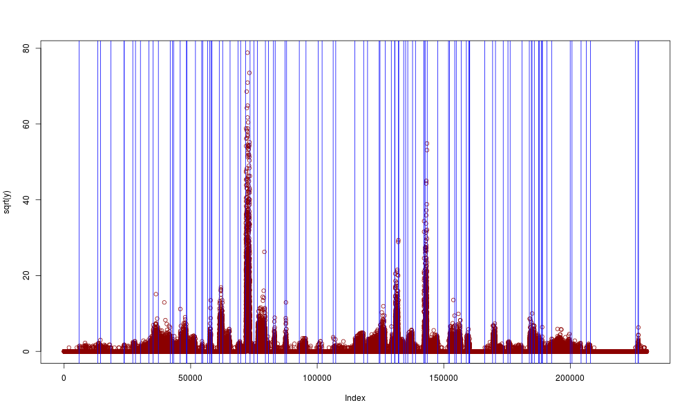
Figure 4 (which is detailed in the Results and discussion section) was obtained with the following $4$ lines of code (assuming the data was contained in vector x):

> Seg<-Segmentor(x,model=3,Kmax=200)

> Kchoose<-SelectModel(Seg, penalty="oracle")

> plot(sqrt(x),col=’dark red’)

> abline(v=getBreaks(Seg)[Kchoose, 1:Kchoose],col=’blue’)

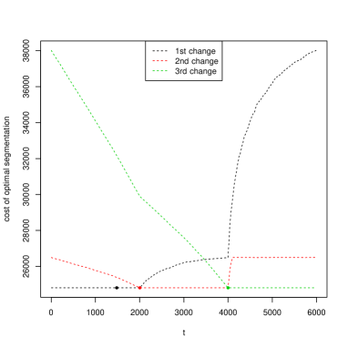
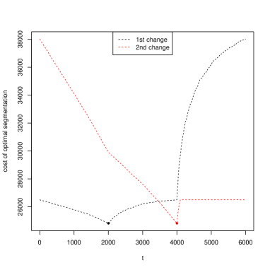
The function BestSegmentation allows, for a given $K$, to find the optimal segmentation with a change-point at location $t$ (slot $bestSeg). It also provides, through the slot $bestCost, the cost of the optimal segmentation with $t$ for $j^{th}$ change-point. Figure 1(b) illustrates this result for the optimal segmentations in $4$ segments of a signal simulated with only $3$ segments. We can see for instance that any choice of first change-point location between $1$ and $2000$ yields almost the same cost (the minimum is obtained for $t=1481$), thus the optimal segmentation is not clearly better than the second or third. On the contrary, the same function with $3$ segments shows that the optimal segmentation outperforms all other segmentations in $3$ segments (Figure 1(a)).

(a) 4 segments

(b) 3 segments

Figure 1: Cost of optimal segmentation in $4$ and $3$ segments. Cost of optimal segmentation depending on the location of the $j^{th}$ change-point when the number of segments is $4$ (figure 1(a)) and $3$ (figure 1(b)) and the signal was simulated with $3$ segments. Illustration of the output of function BestSegmentation.

4 Results and discussion

4.1 Performance study

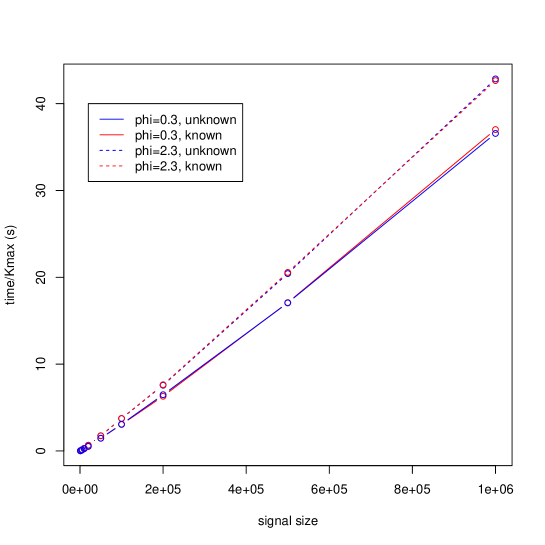
We designed a simulation study on the negative binomial distribution to assess the performance of the PDP algorithm in terms of computational efficiency, while studying the impact of the overdispersion parameter $\phi$ by comparing the results for two different values of this parameter. After running different estimators (median on sliding windows of maximum, quasi-maximum likelihood and moment estimators) on several real RNA-Seq data (whole chromosome and genes of various sizes) we fixed $\phi_{1}=0.3$ as a typical value for highly dispersed data as observed in real RNA-Seq data, and chose $\phi_{2}=2.3$ for comparison with a reasonably dispersed data-set. For each value, we simulated data-sets of size $n$ with various densities of number of segments $K$, and only two possible values for the parameter $p_{J}$: $0.8$ on even segments (corresponding to low signal) and $0.2$ on odd segments for a higher signal. We had $n$ vary on a logarithmic scale between $10^{3}$ and $10^{6}$ and $K$ between $\sqrt{n}/6$ and $\sqrt{n}/3$. For each configuration, we segmented the signal up to $K_{\max}=\sqrt{n}$ twice: once with the known value of $\phi$ and once with our estimator $\widehat{\phi}$ as described above. We started with a window width $h=15$. When the estimate was negative, we doubled $h$ and repeated the experience until the median is positive.

Each configuration was simulated $100$ times.

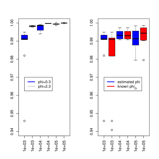
For our analysis we checked the run-time on a standard laptop, and assessed the quality of the segmentation using the Rand Index $\mathcal{I}$. Specifically, let $C_{t}$ be the true index of the segment to which base $t$ belongs and let $\hat{C}_{t}$ be the index estimated by the method, then

$$\mathcal{I}=\frac{2\sum_{t>s}\left[\mathbf{1}_{C_{t}=C_{s}}\mathbf{1}_{\hat{C}_{t}=\hat{C}_{s}}+\mathbf{1}_{C_{t}\neq C_{s}}\mathbf{1}_{\hat{C}_{t}\neq\hat{C}_{s}}\right]}{(n-1)(n-2)}.$$

Figure 2 shows, for the particular case of $K=\sqrt{n}/3$, the almost linear complexity of the algorithm in the size $n$ of the signal. As the maximal number of segments $K_{\max}$ considered increased with $n$, we normalized the run-time to allow comparison. This underlines an empirical complexity smaller than $\mathcal{O}(K_{\max}n\log n)$, and independent on the value of $\phi$ or its knowledge. Moreover, the algorithm, and therefore the pruning, is faster when the overdispersion is high, phenomenon already encountered with the $L^{2}$ loss when the distribution of the errors is Cauchy. However, the knowledge of $\phi$ does not affect the run-time of the algorithm. Figure 3 illustrates through the Rand Index the quality of the proposed segmentation for a few values of $n$. Even though the indexes are slightly lower for $\phi_{1}$ than for $\phi_{2}$ (see left panel), they range between $0.94$ and $1$ showing a great quality in the results. Moreover, the knowledge of $\phi$ does not increase the quality (see right panel), which validates the use of our estimator.

Figure 2: Run-time analysis for segmentation with negative binomial distribution.This figure displays the normalized (by $K_{\max}$) run-time in seconds of the Segmentor3IsBack package for the segmentation of signals with increasing length $n$, for two values of the dispersion $\phi$, and with separate analysis when its value is known or estimated. While the algorithm is faster for more over-dispersed data, the estimation of the parameter does not slow the processing.

Figure 3: Rand-Index for the quality of the segmentation. This figure displays the boxplot of the Rand-index computed for each of the hundred simulations performed in the following situations: comparing the values with $\phi_{1}$ and $\phi_{2}$ when estimated (left figure), and comparing the impact of estimating $\phi_{1}$ (right figure). While the estimation does not decrease the quality of the segmentation, the value of the dispersion affects the recovery of the true change-points.

4.2 Yeast RNAseq experiment

We applied our algorithm to the segmentation of chromosome $1$ of the S. Cerevisiae (yeast) using RNA-Seq data from the Sherlock Laboratory at Stanford University Risso et al. (2011) and publicly available from the NCBI’s Sequence Read Archive (SRA, http://www.ncbi.nlm.nih.gov/sra, accession number SRA048710). We selected the number of segments using our oracle penalty described in the previous section. An existing annotation is available on the Saccharomyces Genome Database (SGD) at http://www.yeastgenome.org, which allows us to validate our results.
With a run-time of $25$ minutes (for a signal length of $230218$), we selected $103$ segments with the negative binomial distribution, most of which (all but $3$) were found to surround known genes from the SGD. Figure 4 illustrates the result.

Figure 4: Segmentation of the yeast chromosome 1 using the negative binomial loss. The model selection procedure chooses $K=103$ segments, most of which surround genes given by the SGD annotation.

5 Conclusion

Segmentation has been a useful tool for the analysis of biological data-sets for a few decades. We propose to extend its application with the use of the Pruned Dynamic Programming algorithm for count data-sets such as outputs of sequencing experiments. We show that the negative binomial distribution can be used to model such data-sets on the condition that the overdispersion parameter is known, and proposed an estimator of this parameter that performs well in our segmentation framework.

We propose to choose the number of segments using our oracle penalty criterion, which makes the package fully operational. This package also allows the use of other criteria such as AIC or BIC. Similarly, the algorithm is not restricted to the negative binomial distribution but also allows the use of Poisson and Gaussian losses for instance, and could easily be adapted to other convex one-parameter losses.

With its empirical complexity of $\mathcal{O}(K_{\max}n\log n)$, it can be applied to large signals such as read-alignment of whole chromosomes, and we illustrated its result on a real-data sets from the yeast genomes. Moreover, this algorithm can be used as a base for further analysis. For example, Luong et al. (2012) use it to initialize their Hidden Markov Model to compute change-point location probabilities.

References

- Akaike [1974] Hirotugu Akaike. A new look at the statistical model identification. Automatic Control, IEEE Transactions on, 19(6):716–723, 1974.
- Arlot and Massart [2009] Sylvain Arlot and Pascal Massart. Data-driven calibration of penalties for least-squares regression. J. Mach. Learn. Res., 10:245–279 (electronic), 2009. URL http://www.jmlr.org/papers/volume10/arlot09a/arlot09a.pdf[pdf].
- Bockhorst and Jojic [2007] J. Bockhorst and N. Jojic. Discovering patterns in biological sequences by optimal segmentation. In Proceedings of the 23rd Conference in Uncertainty in Artificial Intelligence, 2007.
- Boeva et al. [2011] Valentina Boeva, Andrei Zinovyev, Kevin Bleakley, Jean-Philippe Vert, Isabelle Janoueix-Lerosey, Olivier Delattre, and Emmanuel Barillot. Control-free calling of copy number alterations in deep-sequencing data using gc-content normalization. Bioinformatics (Oxford, England), 27:268–9, 2011 Jan 15 2011.
- Braun and Muller [1998] J. V. Braun and H-G Muller. Statistical methods for dna sequence segmentation. Statistical Science, 13(2):142–162, 1998. ISSN 1367-4803.
- Chiang et al. [2009] D. Y. Chiang, G. Getz, D. B. Jaffe, M. J. O’Kelly, X. Zhao, S. L. Carter, C. Russ, C. Nusbaum, M. Meyerson, and E. S. Lander. High-resolution mapping of copy-number alterations with massively parallel sequencing. Nature methods, 6:99–103, 2009.
- Cleynen and Lebarbier [2013] Alice Cleynen and Emilie Lebarbier. Segmentation of the poisson and negative binomial rate models: a penalized estimator. arXiv preprint arXiv:1301.2534, 2013.
- Durot et al. [2009] C. Durot, E. Lebarbier, and A.-S. Tocquet. Estimating the joint distribution of independent categorical variables via model selection. Bernoulli, 15:475–507, 2009.
- Erdman and Emerson [2008] C. Erdman and J. W. Emerson. A fast bayesian change point analysis for the segmentation of microarray data. Bioinformatics, 24(19):2143–2148, 2008.
- Franke et al. [2012] Jurgen Franke, Claudia Kirch, and Joseph Tadjuidje Kamgaing. Changepoints in times series of counts. Journal of Time Series Analysis, 33(5):757–770, 2012.
- [11] Toby Dylan Hocking. Learning smoothing models of copy number profiles using breakpoint annotations. URL hal.inria.fr/hal-00663790.
- Johnson et al. [2005] N. Johnson, A.W. Kemp, and S. Kotz. Univariate discrete distributions. John Wiley & Sons, Inc., 2005.
- Killick et al. [2012] Rebecca Killick, Paul Fearnhead, and IA Eckley. Optimal detection of changepoints with a linear computational cost. Journal of the American Statistical Association, 107(500):1590–1598, 2012.
- Lebarbier [2005] E. Lebarbier. Detecting multiple change-points in the mean of gaussian process by model selection. Signal Processing, 85(4):717–736, April 2005. ISSN 0165-1684. doi: 10.1016/j.sigpro.2004.11.012. URL http://www.sciencedirect.com/science/article/B6V18-4F31YRJ-1/2/b5f7fc37%d9bd95b508c38d4d33fd6c7c.
- Luong et al. [2012] T.M. Luong, Y. Rozenholc, and G. Nuel. Fast estimation of posterior probabilities in change-point models through a constrained hidden markov model. Arxiv preprint arXiv:1203.4394, 2012.
- Olshen et al. [2004] Adam B Olshen, E S Venkatraman, Robert Lucito, and Michael Wigler. Circular binary segmentation for the analysis of array-based DNA copy number data. Biostatistics (Oxford, England), 5(4):557–572, October 2004. ISSN 1465-4644.
- Picard et al. [2011] F. Picard, E. Lebarbier, M. Hoebeke, G. Rigaill, B. Thiam, and S. Robin. Joint segmentation, calling and normalization of multiple cgh profiles. Biostatistics, 12(3):413–428, 2011.
- Picard et al. [2005] Franck Picard, Stephane Robin, Marc Lavielle, Christian Vaisse, and Jean-Jacques Daudin. A statistical approach for array CGH data analysis. BMC Bioinformatics, 6:27, 2005. ISSN 1471-2105.
- Rigaill [2010] G. Rigaill. Pruned dynamic programming for optimal multiple change-point detection. Arxiv:1004.0887, April 2010. URL http://arxiv.org/abs/1004.0887.
- Risso et al. [2011] Davide Risso, Katja Schwartz, Gavin Sherlock, and Sandrine Dudoit. GC-content normalization for RNA-Seq data. BMC Bioinformatics, 12(1):480, 2011.
- Rivera and Walther [2012] Camilo Rivera and Guenther Walther. Optimal detection of a jump in the intensity of a poisson process or in a density with likelihood ratio statistics. arXiv preprint arXiv:1211.2859, 2012.
- Shen and Zhang [2012] Jeremy J. Shen and Nancy R. Zhang. Change-point model on nonhomogeneous poisson processes with application in copy number profiling by next-generation dna sequencing. Annals of Applied Statistics, 6(2):476–496, 2012. doi: http://dx.doi.org/10.1214/11-AOAS517. URL http://projecteuclid.org/euclid.aoas/1339419604.
- Xie and Tammi [2009] C. Xie and M. T. Tammi. CNV-seq, a new method to detect copy number variation using high-throughput sequencing. BMC bioinformatics, 10, 2009.
- Yao [1984] Yi-Ching Yao. Estimation of a noisy Discrete-Time step function: Bayes and empirical bayes approaches. The Annals of Statistics, 12(4):1434–1447, 1984. URL http://projecteuclid.org/DPubS?service=UI&version=1.0&verb=Display&hand%%****␣manuscript.bbl␣Line␣175␣****le=euclid.aos/1176346802.
- Yoon et al. [2009] S. Yoon, Z. Xuan, V. Makarov, K. Ye, and J. Sebat. Sensitive and accurate detection of copy number variants using read depth of coverage. Genome Research, 19:1586–1592, 2009.
- Zhang and Siegmund [2007] Nancy R Zhang and David O Siegmund. A modified bayes information criterion with applications to the analysis of comparative genomic hybridization data. Biometrics, 63(1):22–32, March 2007. ISSN 0006-341X. doi: 10.1111/j.1541-0420.2006.00662.x. URL http://www.ncbi.nlm.nih.gov/pubmed/17447926. PMID: 17447926.
- Zhang et al. [2012] Zhongyang Zhang, Kennenth Lange, and Chiara Sabatti. Reconstructing DNA copy number by joint segmentation of multiple sequences. BMC Bioinformatics, 13(1):205, 2012.