Endogeneity in high dimensions

Abstract

Most papers on high-dimensional statistics are based on the assumption that none of the regressors are correlated with the regression error, namely, they are exogenous. Yet, endogeneity can arise incidentally from a large pool of regressors in a high-dimensional regression. This causes the inconsistency of the penalized least-squares method and possible false scientific discoveries. A necessary condition for model selection consistency of a general class of penalized regression methods is given, which allows us to prove formally the inconsistency claim. To cope with the incidental endogeneity, we construct a novel penalized focused generalized method of moments (FGMM) criterion function. The FGMM effectively achieves the dimension reduction and applies the instrumental variable methods. We show that it possesses the oracle property even in the presence of endogenous predictors, and that the solution is also near global minimum under the over-identification assumption. Finally, we also show how the semi-parametric efficiency of estimation can be achieved via a two-step approach.

T1Supported by NSF Grant DMS-12-06464 and the National Institute of General Medical Sciences of the National Institutes of Health through Grant Numbers R01GM100474 and R01-GM072611.

and

1 Introduction

In high-dimensional models, the overall number of regressors $p$ grows extremely fast with the sample size $n$. It can be of order $\exp(n^{\alpha})$, for some $\alpha\in(0,1)$. What makes statistical inference possible is the sparsity and exogeneity assumptions. For example, in the linear model

$$Y=\mathbf{X}^{T}\bolds{\beta}_{0}+\varepsilon,$$ (1)

it is assumed that the number of elements in $S=\{j\dvtx\beta_{0j}\neq 0\}$ is small and $E\varepsilon\mathbf{X}=0$, or more stringently

$$E(\varepsilon|\mathbf{X})=E\bigl{(}Y-\mathbf{X}^{T}\bolds{\beta}_{0}|\mathbf{X}\bigr{)}=0.$$ (2)

The latter is called “exogeneity.” One of the important objectives of high-dimensional modeling is to achieve the variable selection consistency and make inference on the coefficients of important regressors. See, for example, Fan and Li (2001), Hunter and Li (2005), Zou (2006), Zhao and Yu (2006), Huang, Horowitz and Ma (2008), Zhang and Huang (2008), Wasserman and Roeder (2009), Lv and Fan (2009), Zou and Zhang (2009), Städler, Bühlmann and van de Geer (2010), and Bühlmann, Kalisch and Maathuis (2010). In these papers, (2) (or $E\varepsilon\mathbf{X}=0$) has been assumed either explicitly or implicitly. A condition of this kind is also required by the Dantzig selector of Candès and Tao (2007), which solves an optimization problem with constraint $\max_{j\leq p}|\frac{1}{n}\sum_{i=1}^{n}X_{ij}(Y_{i}-\mathbf{X}_{i}^{T}\bolds{\beta})|<C\sqrt{\frac{\log p}{n}}$ for some $C>0$.

In high-dimensional models, requesting that $\varepsilon$ and all the components of $\mathbf{X}$ be uncorrelated as (2), or even more specifically

$$E\bigl{(}Y-\mathbf{X}^{T}\bolds{\beta}_{0}\bigr{)}X_{j}=0\qquad\forall j=1,\ldots,p,$$ (3)

can be restrictive particularly when $p$ is large. Yet, (3) is a necessary condition for popular model selection techniques to be consistent. However, violations to either assumption (2) or (3) can arise as a result of selection biases, measurement errors, autoregression with autocorrelated errors, omitted variables, and from many other sources [Engle, Hendry and Richard (1983)]. They also arise from unknown causes due to a large pool of regressors, some of which are incidentally correlated with the random noise $Y-\mathbf{X}^{T}\bolds{\beta}_{0}$. For example, in genomics studies, clinical or biological outcomes along with expressions of tens of thousands of genes are frequently collected. After applying variable selection techniques, scientists obtain a set of genes $\widehat{S}$ that are responsible for the outcome. Whether (3) holds, however, is rarely validated. Because there are tens of thousands of restrictions in (3) to validate, it is likely that some of them are violated. Indeed, unlike low-dimensional least-squares, the sample correlations between residuals $\widehat{\varepsilon}$, based on the selected variables $\mathbf{X}_{\widehat{S}}$, and predictors $\mathbf{X}$, are unlikely to be small, because all variables in the large set $\widehat{S}^{c}$ are not even used in computing the residuals. When some of those are unusually large, endogeneity arises incidentally. In such cases, we will show that $\widehat{S}$ can be inconsistent. In other words, violation of assumption (3) can lead to false scientific claims.

We aim to consistently estimate $\bolds{\beta}_{0}$ and recover its sparsity under weaker conditions than (2) or (3) that are easier to validate. Let us assume that $\bolds{\beta}_{0}=(\bolds{\beta}_{0S}^{T},0)^{T}$ and $\mathbf{X}$ can be partitioned as $\mathbf{X}=(\mathbf{X}_{S}^{T},\mathbf{X}_{N}^{T})^{T}$. Here, $\mathbf{X}_{S}$ corresponds to the nonzero coefficients $\bolds{\beta}_{0S}$, which we call important regressors, and $\mathbf{X}_{N}$ represents the unimportant regressors throughout the paper, whose coefficients are zero. We borrow the terminology of endogeneity from the econometric literature. A regressor is said to be endogenous when it is correlated with the error term, and exogenous otherwise. Motivated by the aforementioned issue, this paper aims to select $\mathbf{X}_{S}$ with probability approaching one and making inference about $\bolds{\beta}_{0S}$, allowing components of $\mathbf{X}$ to be endogenous. We propose a unified procedure that can address the problem of endogeneity to be present in either important or unimportant regressors, or both, and we do not require the knowledge of which case of endogeneity is present in the true model. The identities of $\mathbf{X}_{S}$ are unknown before the selection.

The main assumption we make is that there is a vector of observable instrumental variables $\mathbf{W}$ such that

$$E[\varepsilon|\mathbf{W}]=0.$$ (4)

Briefly speaking, $\mathbf{W}$ is called an “instrumental variable” when it satisfies (4) and is correlated with the explanatory variable $\mathbf{X}$. In particular, as noted in the footnote, $\mathbf{W}=\mathbf{X}_{S}$ is allowed so that the instruments are unknown but no additional data are needed. Instrumental variables (IV) have been commonly used in the literature of both econometrics and statistics in the presence of endogenous regressors, to achieve identification and consistent estimations [e.g., Hall and Horowitz (2005)]. An advantage of such an assumption is that it can be validated more easily. For example, when $\mathbf{W}=\mathbf{X}_{S}$, one needs only to check whether the correlations between $\widehat{\varepsilon}$ and $\mathbf{X}_{\widehat{S}}$ are small or not, with $\mathbf{X}_{\widehat{S}}$ being a relatively low-dimensional vector, or more generally, the moments that are actually used in the model fitting such as (5) below hold approximately. In short, our setup weakens the assumption (2) to some verifiable moment conditions.

What makes the variable selection consistency (with endogeneity) possible is the idea of over identification. Briefly speaking, a parameter is called “over-identified” if there are more restrictions than those are needed to grant its identifiability (for linear models, e.g., when the parameter satisfies more equations than its dimension). Let $(f_{1},\ldots,f_{p})$ and $(h_{1},\ldots,h_{p})$ be two different sets of transformations, which can be taken as a large number of series terms, for example, B-splines and polynomials. Here, each $f_{j}$ and $h_{j}$ are scalar functions. Then (4) implies

$$E\bigl{(}\varepsilon f_{j}(\mathbf{W})\bigr{)}=E\bigl{(}\varepsilon h_{j}(\mathbf{W})\bigr{)}=0,\qquad j=1,\ldots,p.$$

Write $\mathbf{F}=(f_{1}(\mathbf{W}),\ldots,f_{p}(\mathbf{W}))^{T}$, and $\mathbf{H}=(h_{1}(\mathbf{W}),\ldots,h_{p}(\mathbf{W}))^{T}$. We then have $E\varepsilon\mathbf{F}=E\varepsilon\mathbf{H}=0$. Let $S$ be the set of indices of important variables, and let $\mathbf{F}_{S}$ and $\mathbf{H}_{S}$ be the subvectors of $\mathbf{F}$ and $\mathbf{H}$ corresponding to the indices in $S$. Implied by $E\varepsilon\mathbf{F}=E\varepsilon\mathbf{H}=0$, and $\varepsilon=Y-\mathbf{X}_{S}^{T}\bolds{\beta}_{0S}$, there exists a solution $\bolds{\beta}_{S}=\bolds{\beta}_{0S}$ to the over-identified equations (with respect to $\bolds{\beta}_{S}$) such as

$$E\bigl{(}Y-\mathbf{X}_{S}^{T}\bolds{\beta}_{S}\bigr{)}\mathbf{F}_{S}=0\quad\mbox{and}\quad E\bigl{(}Y-\mathbf{X}_{S}^{T}\bolds{\beta}_{S}\bigr{)}\mathbf{H}_{S}=0.$$ (5)

In (5), we have twice as many linear equations as the number of unknowns, yet the solution exists and is given by $\bolds{\beta}_{S}=\bolds{\beta}_{0S}$. Because $\bolds{\beta}_{0S}$ satisfies more equations than its dimension, we call $\bolds{\beta}_{0S}$ to be over-identified. On the other hand, for any other set $\tilde{S}$ of variables, if $S\not\subset\tilde{S}$, then the following $2|\tilde{S}|$ equations [with $|\tilde{S}|=\dim(\bolds{\beta}_{\tilde{S}})$ unknowns]

$$E\bigl{(}Y-\mathbf{X}_{\tilde{S}}^{T}\bolds{\beta}_{\tilde{S}}\bigr{)}\mathbf{F}_{\tilde{S}}=0\quad\mbox{and}\quad E\bigl{(}Y-\mathbf{X}_{\tilde{S}}^{T}\bolds{\beta}_{\tilde{S}}\bigr{)}\mathbf{H}_{\tilde{S}}=0$$ (6)

have no solution as long as the basis functions are chosen such that $\mathbf{F}_{\tilde{S}}\neq\mathbf{H}_{\tilde{S}}$. The above setup includes $\mathbf{W}=\mathbf{X}_{S}$ with $\mathbf{F}=\mathbf{X}$ and $\mathbf{H}=\mathbf{X}^{2}$ as a specific example [or $\mathbf{H}=\cos(\mathbf{X})+1$ if $\mathbf{X}$ contain many binary variables].

We show that in the presence of endogenous regressors, the classical penalized least squares method is no longer consistent. Under model

$$Y=\mathbf{X}_{S}^{T}\bolds{\beta}_{0S}+\varepsilon,\qquad E(\varepsilon|\mathbf{W})=0,$$

we introduce a novel penalized method, called focused generalized method of moments (FGMM), which differs from the classical GMM [Hansen (1982)] in that the working instrument $\mathbf{V}(\bolds{\beta})$ in the moment functions $n^{-1}\sum_{i=1}^{n}(Y_{i}-\mathbf{X}_{i}^{T}\bolds{\beta})\mathbf{V}(\bolds{\beta})$ for FGMM also depends irregularly on the unknown parameter $\bolds{\beta}$ [which also depends on $(\mathbf{F},\mathbf{H})$, see Section 3 for details]. With the help of over identification, the FGMM successfully eliminates those subset $\tilde{S}$ such that $S\not\subset\tilde{S}$. As we will see in Section 3, a penalization is still needed to avoid over-fitting. This results in a novel penalized FGMM.

We would like to comment that FGMM differs from the low-dimensional techniques of either moment selection [Andrews (1999), Andrews and Lu (2001)] or shrinkage GMM [Liao (2013)] in dealing with misspecifications of moment conditions and dimension reductions. The existing methods in the literature on GMM moment selections cannot handle high-dimensional models. Recent literature on the instrumental variable method for high-dimensional models can be found in, for example, Belloni et al. (2012), Caner and Fan (2012), García (2011). In these papers, the endogenous variables are in low dimensions. More closely related work is by Gautier and Tsybakov (2011), who solved a constrained minimization as an extension of Dantzig selector. Our paper, in contrast, achieves the oracle property via a penalized GMM. Also, we study a more general conditional moment restricted model that allows nonlinear models.

The remainder of this paper is as follows: Section 2 gives a necessary condition for a general penalized regression to achieve the oracle property. We also show that in the presence of endogenous regressors, the penalized least squares method is inconsistent. Section 3 constructs a penalized FGMM, and discusses the rationale of our construction. Section 4 shows the oracle property of FGMM. Section 5 discusses the global optimization. Section 6 focuses on the semiparametric efficient estimation after variable selection. Section 7 discusses numerical implementations. We present simulation results in Section 8. Finally, Section 9 concludes. Proofs are given in the Appendix.

Notation. Throughout the paper, let $\lambda_{\min}(\mathbf{A})$ and $\lambda_{\max}(\mathbf{A})$ be the smallest and largest eigenvalues of a square matrix $\mathbf{A}$. We denote by $\|\mathbf{A}\|_{F}$, $\|\mathbf{A}\|$ and $\|\mathbf{A}\|_{\infty}$ as the Frobenius, operator and element-wise norms of a matrix $\mathbf{A}$, respectively, defined respectively as $\|\mathbf{A}\|_{F}=\operatorname{tr}^{1/2}(\mathbf{A}^{T}\mathbf{A})$, $\|\mathbf{A}\|=\lambda_{\max}^{1/2}(\mathbf{A}^{T}\mathbf{A})$, and $\|\mathbf{A}\|_{\infty}=\max_{i,j}|\mathbf{A}_{ij}|$. For two sequences $a_{n}$ and $b_{n}$, write $a_{n}\ll b_{n}$ (equivalently, $b_{n}\gg a_{n}$) if $a_{n}=o(b_{n})$. Moreover, $|\bolds{\beta}|_{0}$ denotes the number of nonzero components of a vector $\bolds{\beta}$. Finally, $P_{n}^{\prime}(t)$ and $P^{\prime\prime}_{n}(t)$ denote the first and second derivatives of a penalty function $P_{n}(t)$, if exist.

2 Necessary condition for variable selection consistency

2.1 Penalized regression and necessary condition

Let $s$ denote the dimension of the true vector of nonzero coefficients $\bolds{\beta}_{0S}$. The sparse structure assumes that $s$ is small compared to the sample size. A penalized regression problem, in general, takes a form of

$$\min_{\bolds{\beta}\in\mathbb{R}^{p}}L_{n}(\bolds{\beta})+\sum_{j=1}^{p}P_{n}\bigl{(}|\beta_{j}|\bigr{)},$$

where $P_{n}(\cdot)$ denotes a penalty function. There are relatively less attentions to the necessary conditions for the penalized estimator to achieve the oracle property. Zhao and Yu (2006) derived an almost necessary condition for the sign consistency, which is similar to that of Zou (2006) for the least squares loss with Lasso penalty. To the authors’ best knowledge, so far there has been no necessary condition on the loss function for the selection consistency in the high-dimensional framework. Such a necessary condition is important, because it provides us a way to justify whether a specific loss function can result in a consistent variable selection.

Theorem 2.1 ((Necessary condition))

Suppose: [(iii)]

$L_{n}(\bolds{\beta})$ is twice differentiable, and

$$\max_{1\leq l,j\leq p}\biggl{|}\frac{\partial^{2}L_{n}(\bolds{\beta}_{0})}{\partial\beta_{l}\,\partial\beta_{j}}\biggr{|}=O_{p}(1).$$

There is a local minimizer $\widehat{\bolds{\beta}}=(\widehat{\bolds{\beta}}_{S},\widehat{\bolds{\beta}}_{N})^{T}$ of

$$L_{n}(\bolds{\beta})+\sum_{j=1}^{p}P_{n}\bigl{(}|\beta_{j}|\bigr{)}$$

such that $P(\widehat{\bolds{\beta}}_{N}=0)\rightarrow 1$, and $\sqrt{s}\|\widehat{\bolds{\beta}}-\bolds{\beta}_{0}\|=o_{p}(1)$.

The penalty satisfies: $P_{n}(\cdot)\geq 0$, $P_{n}(0)=0$, $P_{n}^{\prime}(t)$ is nonincreasing when $t\in(0,u)$ for some $u>0$, and $\lim_{n\rightarrow\infty}\lim_{t\rightarrow 0^{+}}P_{n}^{\prime}(t)=0$.

Then for any $l\leq p$,

$$\biggl{|}\frac{\partial L_{n}(\bolds{\beta}_{0})}{\partial\beta_{l}}\biggr{|}\rightarrow^{p}0.$$ (7)

The implication (7) is fundamentally different from the “irrepresentable condition” in Zhao and Yu (2006) and that of Zou (2006). It imposes a restriction on the loss function $L_{n}(\cdot)$, whereas the “irrepresentable condition” is derived under the least squares loss and $E(\varepsilon\mathbf{X})=0$. For the least squares, (7) reduces to either $n^{-1}\sum_{i=1}^{n}\varepsilon_{i}X_{il}=o_{p}(1)$ or $E\varepsilon X_{l}=0$, which requires a exogenous relationship between $\varepsilon$ and $\mathbf{X}$. In contrast, the irrepresentable condition requires a type of relationship between important and unimportant regressors and is specific to Lasso. It also differs from the Karush–Kuhn–Tucker (KKT) condition [e.g., Fan and Lv (2011)] in that it is about the gradient vector evaluated at the true parameters rather than at the local minimizer.

The conditions on the penalty function in condition (iii) are very general, and are satisfied by a large class of popular penalties, such as Lasso [Tibshirani (1996)], SCAD [Fan and Li (2001)] and MCP [Zhang (2010)], as long as their tuning parameter $\lambda_{n}\rightarrow 0$. Hence, this theorem should be understood as a necessary condition imposed on the loss function instead of the penalty.

2.2 Inconsistency of least squares with endogeneity

As an application of Theorem 2.1, consider a linear model:

$$Y=\mathbf{X}^{T}\bolds{\beta}_{0}+\varepsilon=\mathbf{X}_{S}^{T}\bolds{\beta}_{0S}+\varepsilon,$$ (8)

where we may not have $E(\varepsilon\mathbf{X})=0$.

The conventional penalized least squares (PLS) problem is defined as

$$\min_{\bolds{\beta}}\frac{1}{n}\sum_{i=1}^{n}\bigl{(}Y_{i}-\mathbf{X}_{i}^{T}\bolds{\beta}\bigr{)}^{2}+\sum_{j=1}^{p}P_{n}\bigl{(}|\beta_{j}|\bigr{)}.$$

In the simpler case when $s$, the number of nonzero components of $\bolds{\beta}_{0}$, is bounded, it can be shown that if there exist some regressors correlated with the regression error $\varepsilon$, the PLS does not achieve the variable selection consistency. This is because (7) does not hold for the least squares loss function. Hence without the possibly ad-hoc exogeneity assumption, PLS would not work any more, as more formally stated below.

Theorem 2.2 ((Inconsistency of PLS))

Suppose the data are i.i.d., $s=O(1)$, and $\mathbf{X}$ has at least one endogenous component, that is, there is $l$ such that $|E(X_{l}\varepsilon)|>c$ for some $c>0$. Assume that $EX_{l}^{4}<\infty$, $E\varepsilon^{4}<\infty$, and $P_{n}(t)$ satisfies the conditions in Theorem 2.1. If $\tilde{\bolds{\beta}}=(\tilde{\bolds{\beta}}{}^{T}_{S},\tilde{\bolds{\beta}}{}^{T}_{N})^{T}$, corresponding to the coefficients of $(\mathbf{X}_{S},\mathbf{X}_{N})$, is a local minimizer of

$$\frac{1}{n}\sum_{i=1}^{n}\bigl{(}Y_{i}-\mathbf{X}_{i}^{T}\bolds{\beta}\bigr{)}^{2}+\sum_{j=1}^{p}P_{n}\bigl{(}|\beta_{j}|\bigr{)},$$

then either $\|\tilde{\bolds{\beta}}_{S}-\bolds{\beta}_{0S}\|\neq o_{p}(1)$, or $\limsup_{n\rightarrow\infty}P(\tilde{\bolds{\beta}}_{N}=0)<1$.

The index $l$ in the condition of the above theorem does not have to be an index of an important regressor. Hence, the consistency for penalized least squares will fail even if the endogeneity is only present on the unimportant regressors.

We conduct a simple simulated experiment to illustrate the impact of endogeneity on the variable selection. Consider

$$Y = \mathbf{X}^{T}\bolds{\beta}_{0}+\varepsilon,\qquad\varepsilon\sim N(0,1),$$

$$\bolds{\beta}_{0S} = (5,-4,7,-2,1.5);\qquad\beta_{0j}=0\qquad\mbox{for }6\leq j\leq p.$$

$$X_{j} = Z_{j}\qquad\mbox{for }j\leq 5,\qquad X_{j}=(Z_{j}+5)(1+\varepsilon)\qquad\mbox{for }6\leq j\leq p.$$

$$Z \sim N_{p}(0,\Sigma)\qquad\mbox{independent of }\varepsilon,\mbox{ with}(\Sigma)_{ij}=0.5^{|i-j|}.$$

In the design, the unimportant regressors are endogenous. The penalized least squares (PLS) with SCAD-penalty was used for variable selection. The $\lambda$’s in the table represent the tuning parameter used in the SCAD-penalty. The results are based on the estimated $(\widehat{\bolds}{\beta}{}^{T}_{S},\widehat{\bolds}{\beta}{}^{T}_{N})^{T}$, obtained from minimizing PLS and FGMM loss functions, respectively (we shall discuss the construction of FGMM loss function and its numerical minimization in detail subsequently). Here, $\widehat{\bolds}{\beta}_{S}$ and $\widehat{\bolds}{\beta}_{N}$ represent the estimators for coefficients of important and unimportant regressors, respectively.

From Table 1, PLS selects many unimportant regressors (FP). In contrast, the penalized FGMM performs well in both selecting the important regressors and eliminating the unimportant ones. Yet, the larger MSE_S of $\widehat{\bolds{\beta}}_{S}$ by FGMM is due to the moment conditions used in the estimate. This can be improved further in Section 6. Also, when endogeneity is present on the important regressors, PLS estimator will have larger bias (see additional simulation results in Section 8).

Table 1: Performance of PLS and FGMM over 100 replications. $p=50$, $n=200$

	PLS				FGMM
	$\bolds{\lambda=0.05}$	$\bolds{\lambda=0.1}$	$\bolds{\lambda=0.5}$	$\bolds{\lambda=1}$	$\bolds{\lambda=0.05}$	$\bolds{\lambda=0.1}$	$\bolds{\lambda=0.2}$
MSES	0.145	0.133	0.629	1.417	0.261	0.184	0.194
	(0.053)	(0.043)	(0.301)	(0.329)	(0.094)	(0.069)	(0.076)
MSEN	0.126	0.068	0.072	0.095	0.001	0	0.001
	(0.035)	(0.016)	(0.016)	(0.019)	(0.010)	(0)	(0.009)
TP	5	5	4.82	3.63	5	5	5
	(0)	(0)	(0.385)	(0.504)	(0)	(0)	(0)
FP	37.68	35.36	8.84	2.58	0.08	0	0.02
	(2.902)	(3.045)	(3.334)	(1.557)	(0.337)	(0)	(0.141)

[]MSE_S is the average of $\|\widehat{\bolds{\beta}}_{S}-\bolds{\beta}_{0S}\|$ for nonzero coefficients. MSE_N is the average of $\|\widehat{\bolds{\beta}}_{N}-\bolds{\beta}_{0N}\|$ for zero coefficients. TP is the number of correctly selected variables, and FP is the number of incorrectly selected variables. The standard error of each measure is also reported.

3 Focused GMM

3.1 Definition

Because of the presence of endogenous regressors, we introduce an instrumental variable (IV) regression model. Consider a more general nonlinear model:

$$E\bigl{[}g\bigl{(}Y,\mathbf{X}_{S}^{T}\bolds{\beta}_{0S}\bigr{)}|\mathbf{W}\bigr{]}=0,$$ (9)

where $Y$ stands for the dependent variable; $g\dvtx\mathbb{R}\times\mathbb{R}\rightarrow\mathbb{R}$ is a known function. For simplicity, we require $g$ be one-dimensional, and should be thought of as a possibly nonlinear residual function. Our result can be naturally extended to a multidimensional $g$ function. Here, $\mathbf{W}$ is a vector of observed random variables, known as instrumental variables.

Model (9) is called a conditional moment restricted model, which has been extensively studied in the literature, for example, Newey (1993), Donald, Imbens and Newey (2009) and Kitamura, Tripathi and Ahn (2004). The high-dimensional model is also closely related to the semi/nonparametric model estimated by sieves with a growing sieve dimension, for example, Ai and Chen (2003). Recently, van de Geer (2008) and Fan and Lv (2011) considered generalized linear models without endogeneity. Some interesting examples of the generalized linear model that fit into (9) are:

• linear regression, $g(t_{1},t_{2})=t_{1}-t_{2}$;

• logit model, $g(t_{1},t_{2})=t_{1}-\exp(t_{2})/(1+\exp(t_{2}))$;

• probit model, $g(t_{1},t_{2})=t_{1}-\Phi(t_{2})$ where $\Phi(\cdot)$ denotes the standard normal cumulative distribution function.

Let $(f_{1},\ldots,f_{p})$ and $(h_{1},\ldots,h_{p})$ be two different sets of transformations of $\mathbf{W}$, which can be taken as a large number of series basis, for example, B-splines, Fourier series, polynomials [see Chen (2007) for discussions of the choice of sieve functions]. Here, each $f_{j}$ and $h_{j}$ are scalar functions. Write $\mathbf{F}=(f_{1}(\mathbf{W}),\ldots,f_{p}(\mathbf{W}))^{T}$, and $\mathbf{H}=(h_{1}(\mathbf{W}),\ldots,h_{p}(\mathbf{W}))^{T}$. The conditional moment restriction (9) then implies that

$$E\bigl{[}g\bigl{(}Y,\mathbf{X}_{S}^{T}\bolds{\beta}_{0S}\bigr{)}\mathbf{F}_{S}\bigr{]}=0\quad\mbox{and}\quad E\bigl{[}g\bigl{(}Y,\mathbf{X}_{S}^{T}\bolds{\beta}_{0S}\bigr{)}\mathbf{H}_{S}\bigr{]}=0,$$ (10)

where $\mathbf{F}_{S}$ and $\mathbf{H}_{S}$ are the subvectors of $\mathbf{F}$ and $\mathbf{H}$ whose supports are on the oracle set $S=\{j\leq p\dvtx\beta_{0j}\neq 0\}$. In particular, when all the components of $\mathbf{X}_{S}$ are known to be exogenous, we can take $\mathbf{F}=\mathbf{X}$ and $\mathbf{H}=\mathbf{X}^{2}$ (the vector of squares of $\mathbf{X}$ taken coordinately), or $\mathbf{H}=\cos(\mathbf{X})+1$ if $\mathbf{X}$ is a binary variable. A typical estimator based on moment conditions like (10) can be obtained via the generalized method of moments [GMM, Hansen (1982)]. However, in the problem considered here, (10) cannot be used directly to construct the GMM criterion function, because the identities of $\mathbf{X}_{S}$ are unknown.

Remark 3.1.

One seemingly working solution is to define $\mathbf{V}$ as a vector of transformations of $\mathbf{W}$, for instance, $\mathbf{V}=\mathbf{F}$, and employ GMM to the moment condition $E[g(Y,\mathbf{X}^{T}\bolds{\beta}_{0})\mathbf{V}]=0$. However, one has to take $\dim(\mathbf{V})\geq\dim(\bolds{\beta})=p$ to guarantee that the GMM criterion function has a unique minimizer (in the linear model for instance). Due to $p\gg n$, the dimension of $\mathbf{V}$ is too large, and the sample analogue of the GMM criterion function may not converge to its population version due to the accumulation of high-dimensional estimation errors.

Let us introduce some additional notation. For any $\bolds{\beta}\in\mathbb{R}^{p}/\{0\}$, and $i=1,\ldots,n$, define $r=|\bolds{\beta}|_{0}$-dimensional vectors

$$\mathbf{F}_{i}(\bolds{\beta})=\bigl{(}f_{l_{1}}(\mathbf{W}_{i}),\ldots,f_{l_{r}}(\mathbf{W}_{i})\bigr{)}^{T}\quad\mbox{and}\quad\mathbf{H}_{i}(\bolds{\beta})=\bigl{(}h_{l_{1}}(\mathbf{W}_{i}),\ldots,h_{l_{r}}(\mathbf{W}_{i})\bigr{)}^{T},$$

where $(l_{1},\ldots,l_{r})$ are the indices of nonzero components of $\bolds{\beta}$. For example, if $p=3$ and $\bolds{\beta}=(-1,0,2)^{T}$, then $\mathbf{F}_{i}(\bolds{\beta})=(f_{1}(\mathbf{W}_{i}),f_{3}(\mathbf{W}_{i}))^{T}$, and $\mathbf{H}_{i}(\bolds{\beta})=(h_{1}(\mathbf{W}_{i}),h_{3}(\mathbf{W}_{i}))^{T}$, $i\leq n$.

Our focused GMM (FGMM) loss function is defined as

$$L_{\mathrm{FGMM}}(\bolds{\beta}) = \sum_{j=1}^{p}I_{(\beta_{j}\neq 0)}\Biggl{\{}w_{j1}\Biggl{[}\frac{1}{n}\sum_{i=1}^{n}g\bigl{(}Y_{i},\mathbf{X}_{i}^{T}\bolds{\beta}\bigr{)}f_{j}(\mathbf{W}_{i})\Biggr{]}^{2}$$

$$\hskip 53.0pt{}+w_{j2}\Biggl{[}\frac{1}{n}\sum_{i=1}^{n}g\bigl{(}Y_{i},\mathbf{X}_{i}^{T}\bolds{\beta}\bigr{)}h_{j}(\mathbf{W}_{i})\Biggr{]}^{2}\Biggr{\}},$$

where $w_{j1}$ and $w_{j2}$ are given weights. For example, we will take $w_{j1}=1/\widehat{\operatorname{var}}(f_{j}(\mathbf{W}))$ and $w_{j2}=1/\widehat{\operatorname{var}}(h_{j}(\mathbf{W}))$ to standardize the scale (here $\widehat{\operatorname}{var}$ represents the sample variance). Writing in the matrix form, for $\mathbf{V}_{i}(\bolds{\beta})=(\mathbf{F}_{i}(\bolds{\beta})^{T},\mathbf{H}_{i}(\bolds{\beta})^{T})^{T}$,

$$L_{\mathrm{FGMM}}(\bolds{\beta})=\Biggl{[}\frac{1}{n}\sum_{i=1}^{n}g\bigl{(}Y_{i},\mathbf{X}_{i}^{T}\bolds{\beta}\bigr{)}\mathbf{V}_{i}(\bolds{\beta})\Biggr{]}^{T}\mathbf{J}(\bolds{\beta})\Biggl{[}\frac{1}{n}\sum_{i=1}^{n}g\bigl{(}Y_{i},\mathbf{X}_{i}^{T}\bolds{\beta}\bigr{)}\mathbf{V}_{i}(\bolds{\beta})\Biggr{]},$$

where $\mathbf{J}(\bolds{\beta})=\operatorname{diag}\{w_{l_{1}1},\ldots,w_{l_{r}1},w_{l_{1}2},\ldots,w_{l_{r}2}\}$.

Unlike the traditional GMM, the “working instrumental variables” $\mathbf{V}(\bolds{\beta})$ depend irregularly on the unknown $\bolds{\beta}$. As to be further explained, this ensures the dimension reduction, and allows to focus only on the equations with the IV whose support is on the oracle space, and is therefore called the focused GMM or FGMM for short.

We then define the FGMM estimator by minimizing the following criterion function:

$$Q_{\mathrm{FGMM}}(\bolds{\beta})=L_{\mathrm{FGMM}}(\bolds{\beta})+\sum_{j=1}^{p}P_{n}\bigl{(}|\beta_{j}|\bigr{)}.$$ (12)

Sufficient conditions on the penalty function $P_{n}(|\beta_{j}|)$ for the oracle property will be presented in Section 4. Penalization is needed because otherwise small coefficients in front of unimportant variables would be still kept in minimizing $L_{\mathrm{FGMM}}(\bolds{\beta})$. As to become clearer in Section 6, the FGMM focuses on the model selection and estimation consistency without paying much effort to the efficient estimation of $\bolds{\beta}_{0S}$.

3.2 Rationales behind the construction of FGMM

3.2.1 Inclusion of $\mathbf{V}(\bolds{\beta})$

We construct the FGMM criterion function using

$$\mathbf{V}(\bolds{\beta})=\bigl{(}\mathbf{F}(\bolds{\beta})^{T},\mathbf{H}(\bolds{\beta})^{T}\bigr{)}^{T}.$$

A natural question arises: why not just use one set of IV’s so that $\mathbf{V}(\bolds{\beta})=\mathbf{F}(\bolds{\beta})$? We now explain the rationale behind the inclusion of the second set of instruments $\mathbf{H}(\bolds{\beta})$. To simplify notation, let $F_{ij}=f_{j}(\mathbf{W}_{i})$ and $H_{ij}=h_{j}(\mathbf{W}_{i})$ for $j\leq p$ and $i\leq n$. Then $\mathbf{F}_{i}=(F_{i1},\ldots,F_{ip})$ and $\mathbf{H}_{i}=(H_{i1},\ldots,H_{ip})$. Also, write $F_{j}=f_{j}(\mathbf{W})$ and $H_{j}=h_{j}(\mathbf{W})$ for $j\leq p$.

Let us consider a linear regression model (8) as an example. If $\mathbf{H}(\bolds{\beta})$ were not included and $\mathbf{V}(\bolds{\beta})=\mathbf{F}(\bolds{\beta})$ had been used, the GMM loss function would have been constructed as

$$L_{v}(\bolds{\beta})=\Biggl{\|}\frac{1}{n}\sum_{i=1}^{n}\bigl{(}Y_{i}-\mathbf{X}_{i}^{T}\bolds{\beta}\bigr{)}\mathbf{F}_{i}(\bolds{\beta})\Biggr{\|}^{2},$$ (13)

where for the simplicity of illustration, $\mathbf{J}(\bolds{\beta})$ is taken as an identity matrix. We also use the $L_{0}$-penalty $P_{n}(|\beta_{j}|)=\lambda_{n}I_{(|\beta_{j}|\neq 0)}$ for illustration. Suppose that the true $\bolds{\beta}_{0}=(\bolds{\beta}_{0S}^{T},0,\ldots,0)^{T}$ where only the first $s$ components are nonzero and that $s>1$. If we, however, restrict ourselves to $\bolds{\beta}_{p}=(0,\ldots,0,\beta_{p})$, the criterion function now becomes

$$Q_{\mathrm{FGMM}}(\bolds{\beta}_{p})=\Biggl{[}\frac{1}{n}\sum_{i=1}^{n}(Y_{i}-X_{ip}\beta_{p})F_{ip}\Biggr{]}^{2}+\lambda_{n}.$$

It is easy to see its minimum is just $\lambda_{n}$. On the other hand, if we optimize $Q_{\mathrm{FGMM}}$ on the oracle space $\bolds{\beta}=(\bolds{\beta}_{S}^{T},0)^{T}$, then

$$\min_{\bolds{\beta}=(\bolds{\beta}_{S}^{T},0)^{T},\bolds{\beta}_{S,j}\neq 0}Q_{\mathrm{FGMM}}(\bolds{\beta})\geq s\lambda_{n}.$$

As a result, it is inconsistent for variable selection.

The use of $L_{0}$-penalty is not essential in the above illustration. The problem is still present if the $L_{1}$-penalty is used, and is not merely due to the biasedness of $L_{1}$-penalty. For instance, recall that for the SCAD penalty with hyper parameter $(a,\lambda_{n})$, $P_{n}(\cdot)$ is nondecreasing, and $P_{n}(t)=\frac{(a+1)}{2}\lambda_{n}^{2}$ when $t\geq a\lambda_{n}$. Given that $\min_{j\in S}|\beta_{0j}|\gg\lambda_{n}$,

$$Q_{\mathrm{FGMM}}(\bolds{\beta}_{0})\geq\sum_{j\in S}P_{n}\bigl{(}|\beta_{0j}|\bigr{)}\geq sP_{n}\Bigl{(}\min_{j\in S}|\beta_{0j}|\Bigr{)}=\frac{(a+1)}{2}\lambda_{n}^{2}s.$$

On the other hand, $Q_{\mathrm{FGMM}}(\bolds{\beta}_{p}^{*})=P_{n}(|\beta_{p}^{*}|)\leq\frac{(a+1)}{2}\lambda_{n}^{2}$ which is strictly less than $Q_{\mathrm{FGMM}}(\bolds{\beta}_{0})$. So, the problem is still present when an asymptotically unbiased penalty (e.g., SCAD, MCP) is used.

Including an additional term $\mathbf{H}(\bolds{\beta})$ in $\mathbf{V}(\bolds{\beta})$ can overcome this problem. For example, if we still restrict to $\bolds{\beta}_{p}=(0,\ldots,\beta_{p})$ but include an additional but different IV $H_{ip}$, the criterion function then becomes, for the $L_{0}$ penalty:

$$Q_{\mathrm{FGMM}}(\bolds{\beta}_{p})=\Biggl{[}\frac{1}{n}\sum_{i=1}^{n}(Y_{i}-X_{ip}\beta_{p})F_{ip}\Biggr{]}^{2}+\Biggl{[}\frac{1}{n}\sum_{i=1}^{n}(Y_{i}-X_{ip}\beta_{p})H_{ip}\Biggr{]}^{2}+\lambda_{n}.$$

In general, the first two terms cannot achieve $o_{p}(1)$ simultaneously as long as the two sets of transformations $\{f_{j}(\cdot)\}$ and $\{h_{j}(\cdot)\}$ are fixed differently, so long as $n$ is large and

$$(EX_{p}F_{p})^{-1}E(YF_{p})\neq(EX_{p}H_{p})^{-1}E(YH_{p}).$$ (14)

As a result, $Q_{\mathrm{FGMM}}(\bolds{\beta}_{p})$ is bounded away from zero with probability approaching one.

To better understand the behavior of $Q_{\mathrm{FGMM}}(\bolds{\beta})$, it is more convenient to look at the population analogues of the loss function. Because the number of equations in

$$E\bigl{[}\bigl{(}Y-\mathbf{X}^{T}\bolds{\beta}\bigr{)}\mathbf{F}(\bolds{\beta})\bigr{]}=0\quad\mbox{and}\quad E\bigl{[}\bigl{(}Y-\mathbf{X}^{T}\bolds{\beta}\bigr{)}\mathbf{H}(\bolds{\beta})\bigr{]}=0$$ (15)

is twice as many as the number of unknowns (nonzero components in $\bolds{\beta}$), if we denote $\tilde{S}$ as the support of $\bolds{\beta}$, then (15) has a solution only when $(E\mathbf{F}_{\tilde{S}}\mathbf{X}_{\tilde{S}}^{T})^{-1}E(Y\mathbf{F}_{\tilde{S}})=(E\mathbf{H}_{\tilde{S}}\mathbf{X}_{\tilde{S}}^{T})^{-1}E(Y\mathbf{H}_{\tilde{S}})$, which does not hold in general unless $\tilde{S}=S$, the index set of the true nonzero coefficients. Hence, it is natural for (15) to have a unique solution $\bolds{\beta}=\bolds{\beta}_{0}$. As a result, if we define

$$G(\bolds{\beta})=\bigl{\|}E\bigl{(}Y-\mathbf{X}^{T}\bolds{\beta}\bigr{)}\mathbf{F}(\bolds{\beta})\bigr{\|}^{2}+\bigl{\|}E\bigl{(}Y-\mathbf{X}^{T}\bolds{\beta}\bigr{)}\mathbf{H}(\bolds{\beta})\bigr{\|}^{2},$$

the population version of $L_{\mathrm{FGMM}}$, then as long as $\bolds{\beta}$ is not close to $\bolds{\beta}_{0}$, $G$ should be bounded away from zero. Therefore, it is reasonable for us to assume that for any $\delta>0$, there is $\gamma(\delta)>0$ such that

$$\inf_{\|\bolds{\beta}-\bolds{\beta}_{0}\|_{\infty}>\delta,\bolds{\beta}\neq 0}G(\bolds{\beta})>\gamma(\delta).$$ (16)

On the other hand, $E(\varepsilon|\mathbf{W})=E(Y-\mathbf{X}_{S}^{T}\bolds{\beta}_{0S}|\mathbf{W})=0$ implies $G(\bolds{\beta}_{0})=0$.

Our FGMM loss function is essentially a sample version of $G(\bolds{\beta})$, so minimizing $L_{\mathrm{FGMM}}(\bolds{\beta})$ forces the estimator to be close to $\bolds{\beta}_{0}$, but small coefficients in front of unimportant but exogenous regressors may still be allowed. Hence, a concave penalty function is added to $L_{\mathrm{FGMM}}$ to define $Q_{\mathrm{FGMM}}$.

3.2.2 Indicator function

Another question readers may ask is that why not define $L_{\mathrm{FGMM}}(\bolds{\beta})$ to be, for some weight matrix $\mathbf{J}$,

$$\Biggl{[}\frac{1}{n}\sum_{i=1}^{n}g\bigl{(}Y_{i},\mathbf{X}_{i}^{T}\bolds{\beta}\bigr{)}\mathbf{V}_{i}\Biggr{]}^{T}\mathbf{J}\Biggl{[}\frac{1}{n}\sum_{i=1}^{n}g\bigl{(}Y_{i},\mathbf{X}_{i}^{T}\bolds{\beta}\bigr{)}\mathbf{V}_{i}\Biggr{]},$$ (17)

that is, why not replace the irregular $\bolds{\beta}$-dependent $\mathbf{V}(\bolds{\beta})$ with $\mathbf{V}$, and use the entire $2p$-dimensional $\mathbf{V}=(\mathbf{F}^{T},\mathbf{H}^{T})^{T}$ as the IV? This is equivalent to the question why the indicator function in (3.1) cannot be dropped.

The indicator function is used to prevent the accumulation of estimation errors under the high dimensionality. To see this, rewrite (17) to be

$$\sum_{j=1}^{p}\frac{1}{\widehat{\operatorname{var}}(F_{j})}\Biggl{(}\frac{1}{n}\sum_{i=1}^{n}g\bigl{(}Y_{i},\mathbf{X}_{i}^{T}\bolds{\beta}\bigr{)}F_{ij}\Biggr{)}^{2}+\frac{1}{\widehat{\operatorname{var}}(H_{j})}\Biggl{(}\frac{1}{n}\sum_{i=1}^{n}g\bigl{(}Y_{i},\mathbf{X}_{i}^{T}\bolds{\beta}\bigr{)}H_{ij}\Biggr{)}^{2}.$$

Since $\dim(\mathbf{V}_{i})=2p\gg n$, even if each individual term evaluated at $\bolds{\beta}=\bolds{\beta}_{0}$ is $O_{p}(\frac{1}{n})$, the sum of $p$ terms would become stochastically unbounded. In general, (17) does not converge to its population analogue when $p\gg n$ because the accumulation of high-dimensional estimation errors would have a nonnegligible effect.

In contrast, the indicator function effectively reduces the dimension and prevents the accumulation of estimation errors. Once the indicator function is included, the proposed FGMM loss function evaluated at $\bolds{\beta}_{0}$ becomes

$$\sum_{j\in S}\frac{1}{\widehat{\operatorname{var}}(F_{j})}\Biggl{(}\frac{1}{n}\sum_{i=1}^{n}g\bigl{(}Y_{i},\mathbf{X}_{i}^{T}\bolds{\beta}_{0}\bigr{)}F_{ij}\Biggr{)}^{2}+\frac{1}{\widehat{\operatorname{var}}(H_{j})}\Biggl{(}\frac{1}{n}\sum_{i=1}^{n}g\bigl{(}Y_{i},\mathbf{X}_{i}^{T}\bolds{\beta}_{0}\bigr{)}H_{ij}\Biggr{)}^{2},$$

which is small because $E[g(Y,\mathbf{X}^{T}\bolds{\beta}_{0})\mathbf{F}_{S}]=E[g(Y,\mathbf{X}^{T}\bolds{\beta}_{0})\mathbf{H}_{S}]=0$ and that there are only $s=|S|_{0}$ terms in the summation.

Recently, there has been a growing literature on the shrinkage GMM, for example, Caner (2009), Caner and Zhang (2014), Liao (2013), etc., regarding estimation and variable selection based on a set of moment conditions like (10). The model considered by these authors is restricted to either a low-dimensional parameter space or a low-dimensional vector of moment conditions, where there is no such a problem of error accumulations.

4 Oracle property of FGMM

FGMM involves a nonsmooth loss function. In the Appendix, we develop a general asymptotic theory for high-dimensional models to accommodate the nonsmooth loss function.

Our first assumption defines the penalty function we use. Consider a similar class of folded concave penalty functions as that in Fan and Li (2001).

For any $\bolds{\beta}=(\beta_{1},\ldots,\beta_{s})^{T}\in\mathbb{R}^{s}$, and $|\beta_{j}|\neq 0,j=1,\ldots,s$, define

$$\eta(\bolds{\beta})=\limsup_{\epsilon\rightarrow 0^{+}}\max_{j\leq s}\mathop{\sup_{t_{1}<t_{2}}}_{(t_{1},t_{2})\in(|\beta_{j}|-\epsilon,|\beta_{j}|+\epsilon)}-\frac{P_{n}^{\prime}(t_{2})-P_{n}^{\prime}(t_{1})}{t_{2}-t_{1}},$$ (18)

which is $\max_{j\leq s}-P_{n}^{\prime\prime}(|\beta_{j}|)$ if the second derivative of $P_{n}$ is continuous. Let

$$d_{n}=\tfrac{1}{2}\min\bigl{\{}|\beta_{0j}|\dvtx\beta_{0j}\neq 0,j=1,\ldots,p\bigr{\}}$$

represent the strength of signals.

Assumption 4.1.

The penalty function $P_{n}(t)\dvtx[0,\infty)\rightarrow\mathbb{R}$ satisfies: [(iii)]

$P_{n}(0)=0$.

$P_{n}(t)$ is concave, nondecreasing on $[0,\infty)$, and has a continuous derivative $P_{n}^{\prime}(t)$ when $t>0$.

$\sqrt{s}P_{n}^{\prime}(d_{n})=o(d_{n})$.

There exists $c>0$ such that $\sup_{\bolds{\beta}\in B(\bolds{\beta}_{0S},cd_{n})}\eta(\bolds{\beta})=o(1)$.

These conditions are standard. The concavity of $P_{n}(\cdot)$ implies that $\eta(\bolds{\beta})\geq 0$ for all $\bolds{\beta}\in\mathbb{R}^{s}$. It is straightforward to check that with properly chosen tuning parameters, the $L_{q}$ penalty (for $q\leq 1$), hard-thresholding [Antoniadis (1996)], SCAD [Fan and Li (2001)], and MCP [Zhang (2010)] all satisfy these conditions. As thoroughly discussed by Fan and Li (2001), a penalty function that is desirable for achieving the oracle properties should result in an estimator with three properties: unbiasedness, sparsity and continuity [see Fan and Li (2001) for details]. These properties motivate the needs of using a folded concave penalty.

The following assumptions are further imposed. Recall that for $j\leq p$, $F_{j}=f_{j}(\mathbf{W})$ and $H_{j}=h_{j}(\mathbf{W})$.

Assumption 4.2.

(i) The true parameter $\bolds{\beta}_{0}$ is uniquely identified by $E(g(Y,\mathbf{X}^{T}\bolds{\beta}_{0})|\mathbf{W})=0$.

(ii) $(Y_{1},\mathbf{X}_{1}),\ldots,(Y_{n},\mathbf{X}_{n})$ are independent and identically distributed.

Remark 4.1.

Condition (i) above is standard in the GMM literature [e.g., Newey (1993), Donald, Imbens and Newey (2009), Kitamura, Tripathi and Ahn (2004)]. This condition is closely related to the “over-identifying restriction,” and ensures that we can always find two sets of transformations $\mathbf{F}$ and $\mathbf{H}$ such that the equations in (10) are uniquely satisfied by $\bolds{\beta}_{S}=\bolds{\beta}_{0S}$. In linear models, this is a reasonable assumption, as discussed in Section 3.2. In nonlinear models, however, requiring the identifiability from either $E(g(Y,\mathbf{X}^{T}\bolds{\beta}_{0})|\mathbf{W})=0$ or (10) may be restrictive. Indeed, Dominguez and Lobato (2004) showed that the identification condition in (i) may depend on the marginal distributions of $\mathbf{W}$. Furthermore, in nonparametric regression problems as in Bickel, Ritov and Tsybakov (2009) and Ai and Chen (2003), the sufficient condition of condition (i) is even more complicated, which also depends on the conditional distribution of $\mathbf{X}|\mathbf{W}$, and is known to be statistically untestable [see Newey and Powell (2003), Canay, Santos and Shaikh (2013)].

Assumption 4.3.

There exist $b_{1},b_{2},b_{3}>0$ and $r_{1},r_{2},r_{3}>0$ such that for any $t>0$, [(iii)]

$P(|g(Y,\mathbf{X}^{T}\bolds{\beta}_{0})|>t)\leq\exp(-(t/b_{1})^{r_{1}})$.

$\max_{l\leq p}P(|F_{l}|>t)\leq\exp(-(t/b_{2})^{r_{2}})$, $\max_{l\leq p}P(|H_{l}|>t)\leq\break\exp(-(t/b_{3})^{r_{3}})$.

$\min_{j\in S}\operatorname{var}(g(Y,\mathbf{X}^{T}\bolds{\beta}_{0})F_{j})$ and $\min_{j\in S}\operatorname{var}(g(Y,\mathbf{X}^{T}\bolds{\beta}_{0})H_{j})$ arebounded away from zero.

$\operatorname{var}(F_{j})$ and $\operatorname{var}(H_{j})$ are bounded away from both zero and infinity uniformly in $j=1,\ldots,p$ and $p\geq 1$.

We will assume $g(\cdot,\cdot)$ to be twice differentiable, and in the following assumptions, let

$$m(t_{1},t_{2})=\frac{\partial g(t_{1},t_{2})}{\partial t_{2}},\qquad q(t_{1},t_{2})=\frac{\partial^{2}g(t_{1},t_{2})}{\partial t_{2}^{2}},\qquad\mathbf{V}_{S}=\pmatrix{\mathbf{F}_{S}\vspace*{2pt}\cr\mathbf{H}_{S}}.$$

Assumption 4.4.

(i) $g(\cdot,\cdot)$ is twice differentiable.

(ii) $\sup_{t_{1},t_{2}}|m(t_{1},t_{2})|<\infty$, and $\sup_{t_{1},t_{2}}|q(t_{1},t_{2})|<\infty$.

It is straightforward to verify Assumption 4.4 for linear, logistic and probit regression models.

Assumption 4.5.

There exist $C_{1}>0$ and $C_{2}>0$ such that

$$\lambda_{\max}\bigl{[}\bigl{(}Em\bigl{(}Y,\mathbf{X}_{S}^{T}\bolds{\beta}_{0S}\bigr{)}\mathbf{X}_{S}\mathbf{V}_{S}^{T}\bigr{)}\bigl{(}Em\bigl{(}Y,\mathbf{X}_{S}^{T}\bolds{\beta}_{0S}\bigr{)}\mathbf{X}_{S}\mathbf{V}_{S}^{T}\bigr{)}^{T}\bigr{]} < C_{1},$$

$$\lambda_{\min}\bigl{[}\bigl{(}Em\bigl{(}Y,\mathbf{X}_{S}^{T}\bolds{\beta}_{0S}\bigr{)}\mathbf{X}_{S}\mathbf{V}_{S}^{T}\bigr{)}\bigl{(}Em\bigl{(}Y,\mathbf{X}_{S}^{T}\bolds{\beta}_{0S}\bigr{)}\mathbf{X}_{S}\mathbf{V}_{S}^{T}\bigr{)}^{T}\bigr{]} > C_{2}.$$

These conditions require that the instrument $\mathbf{V}_{S}$ be not weak, that is, $\mathbf{V}_{S}$ should not be weakly correlated with the important regressors. In the generalized linear model, Assumption 4.5 is satisfied if proper conditions on the design matrices are imposed. For example, in the linear regression model and probit model, we assume the eigenvalues of $(E\mathbf{X}_{S}\mathbf{V}_{S}^{T})(E\mathbf{X}_{S}\mathbf{V}_{S}^{T})^{T}$ and $(E\phi(\mathbf{X}^{T}\bolds{\beta}_{0})\mathbf{X}_{S}\mathbf{V}_{S}^{T})(E\phi(\mathbf{X}^{T}\bolds{\beta}_{0})\mathbf{X}_{S}\mathbf{V}_{S}^{T})^{T}$ are bounded away from both zero and infinity respectively, where $\phi(\cdot)$ is the standard normal density function. Conditions in the same spirit are also assumed in, for example, Bradic, Fan and Wang (2011), and Fan and Lv (2011).

Define

$$\bolds{\Upsilon}=\operatorname{var}\bigl{(}g\bigl{(}Y,\mathbf{X}_{S}^{T}\bolds{\beta}_{0S}\bigr{)}\mathbf{V}_{S}\bigr{)}.$$ (19)

Assumption 4.6.

(i) For some $c>0$, $\lambda_{\min}(\bolds{\Upsilon})>c$. [(iii)]

$sP_{n}^{\prime}(d_{n})+s\sqrt{(\log p)/n}+s^{3}(\log s)/n=o(P_{n}^{\prime}(0^{+}))$, $P_{n}^{\prime}(d_{n})s^{2}=O(1)$, and $s\sqrt{(\log p)/n}=o(d_{n})$.

$P_{n}^{\prime}(d_{n})=o(1/\sqrt{ns})$ and $\sup_{\|\bolds{\beta}-\bolds{\beta}_{0S}\|\leq d_{n}/4}\eta(\bolds{\beta})=o((s\log p)^{-1/2})$.

$\max_{j\notin S}\|Em(y,\mathbf{X}^{T}\bolds{\beta}_{0})X_{j}\mathbf{V}_{S}\|\sqrt{(\log s)/n}=o(P_{n}(0^{+}))$.

This assumption imposes a further condition jointly on the penalty, the strength of the minimal signal and the number of important regressors. Condition (i) is needed for the asymptotic normality of the estimated nonzero coefficients. When either SCAD or MCP is used as the penalty function with a tuning parameter $\lambda_{n}$, $P_{n}^{\prime}(d_{n})=\sup_{\|\bolds{\beta}-\bolds{\beta}_{0S}\|\leq d_{n}/4}\eta(\bolds{\beta})=0$ and $P_{n}^{\prime}(0^{+})=\lambda_{n}$ when $\lambda_{n}=o(d_{n})$. Thus, conditions (ii)–(iv) in the assumption are satisfied as long as $s\sqrt{\log p/n}+s^{3}\log s/n\ll\lambda_{n}\ll d_{n}$. This requires the signal $d_{n}$ be strong and $s$ be small compared to $n$. Such a condition is needed to achieve the variable selection consistency.

Under the foregoing regularity conditions, we can show the oracle property of a local minimizer of $Q_{\mathrm{FGMM}}$ (12).

Theorem 4.1

Suppose $s^{3}\log p=o(n)$. Under Assumptions 4.1–4.6, there exists a local minimizer $\widehat{\bolds{\beta}}=(\widehat{\bolds{\beta}}{}^{T}_{S},\widehat{\bolds{\beta}}{}^{T}_{N})^{T}$ of $Q_{\mathrm{FGMM}}(\bolds{\beta})$ with $\widehat{\bolds{\beta}}_{S}$ and $\widehat{\bolds{\beta}}_{N}$ being sub-vectors of $\widehat{\bolds{\beta}}$ whose coordinates are in $S$ and $S^{c}$, respectively, such that

$$\mathrm{(i)}\hskip 100.0pt\sqrt{n}\bolds{\alpha}^{T}\bolds{\Gamma}^{-1/2}\bolds{\Sigma}(\widehat{\bolds{\beta}}_{S}-\bolds{\beta}_{0S})\rightarrow^{d}N(0,1)$$

for any unit vector $\bolds{\alpha}\in\mathbb{R}^{s}$, $\|\bolds{\alpha}\|=1$, where $\mathbf{A}=Em(Y,\mathbf{X}^{T}\bolds{\beta}_{0})\mathbf{X}_{S}\mathbf{V}_{S}^{T}$,

$$\bolds{\Gamma}=4\mathbf{A}\mathbf{J}(\bolds{\beta}_{0})\bolds{\Upsilon}\mathbf{J}(\bolds{\beta}_{0})\mathbf{A}^{T}\quad\mbox{and}\quad\bolds{\Sigma}=2\mathbf{A}\mathbf{J}(\bolds{\beta}_{0})\mathbf{A}^{T}.$$

$$\mathrm{(ii)}\hskip 114.0pt\qquad\lim_{n\rightarrow\infty}P(\widehat{\bolds{\beta}}_{N}=0)=1.$$

In addition, the local minimizer $\widehat{\bolds{\beta}}$ is strict with probability at least $1-\delta$ for an arbitrarily small $\delta>0$ and all large $n$.

(iii) Let $\widehat{S}=\{j\leq p\dvtx\widehat{\beta}_{j}\neq 0\}$. Then

$$P(\widehat{S}=S)\rightarrow 1.$$

Remark 4.2.

As was shown in an earlier version of this paper, Fan and Liao (2012), when it is known that $E[g(Y,\mathbf{X}^{T}\bolds{\beta}_{0})|\mathbf{X}_{S}]=0$ but likely $E[g(Y,\mathbf{X}^{T}\bolds{\beta}_{0})|\mathbf{X}]\neq 0$, we can take $\mathbf{V}=(\mathbf{F}^{T},\mathbf{H}^{T})^{T}$ to be transformations of $\mathbf{X}$ that satisfy Assumptions 4.3–4.6. In this way, we do not need an extra instrumental variable $\mathbf{W}$, and Theorem 4.1 still goes through, while the traditional methods (e.g., penalized least squares in the linear model) can still fail as shown by Theorem 2.2. In the high-dimensional linear model, compared to the classical assumption: $E(\varepsilon|\mathbf{X})=0$, our condition $E(\varepsilon|\mathbf{X}_{S})=0$ is relatively easier to validate as $\mathbf{X}_{S}$ is a low-dimensional vector.

Remark 4.3.

We now explain our required lower bound on the signal $s\sqrt{\log p/n}=o(d_{n})$. When a penalized regression is used, which takes the form $\min_{\bolds{\beta}}L_{n}(\bolds{\beta})+\sum_{j=1}^{p}P_{n}(|\beta_{j}|)$, it is required that if $L_{n}(\bolds{\beta})$ is differentiable, $\max_{j\notin S}|\partial L_{n}(\bolds{\beta}_{0})/\partial\beta_{j}|=o(P_{n}^{\prime}(0^{+}))$. This often leads to a requirement of the lower bound of $d_{n}$. Therefore, such a lower bound of $d_{n}$ depends on the choice of both the loss function $L_{n}(\bolds{\beta})$ and the penalty. For instance, in the linear model when least squares with a SCAD penalty is employed, this condition is equivalent to $\sqrt{\log p/n}=o(d_{n})$. It is also known that the adaptive lasso penalty requires the minimal signal to be significantly larger than $\sqrt{\log p/n}$ [Huang, Ma and Zhang (2008)]. In our framework, the requirement $s\sqrt{\log p/n}=o(d_{n})$ arises from the use of the new FGMM loss function. Such a condition is stronger than that of the least squares loss function, which is the price paid to achieve variable selection consistency in the presence of endogeneity. This condition is still easy to satisfy as long as $s$ grows slowly with $n$.

Remark 4.4.

Similar to the “irrpresentable condition” for Lasso, the FGMM requires important and unimportant explanatory variables not be strongly correlated. This is fulfilled by Assumption 4.6(iv). For instance, in the linear model and $\mathbf{V}_{S}$ contains $\mathbf{X}_{S}$ as in our earlier version, this condition implies $\max_{j\notin S}\|EX_{j}\mathbf{X}_{S}\|\sqrt{\log s/n}=o(\lambda_{n})$. Strong correlation between $(\mathbf{X}_{S},\mathbf{X}_{N})$ is also ruled out by the identifiability condition Assumption 4.2. To illustrate the idea, consider a case of perfect linear correlation: $\mathbf{X}_{S}^{T}\bolds{\alpha}-\mathbf{X}_{N}^{T}\bolds{\delta}=0$ for some $(\bolds{\alpha},\bolds{\delta})$ with $\bolds{\delta}\neq 0$. Then $\mathbf{X}^{T}\bolds{\beta}_{0}=\mathbf{X}_{S}^{T}(\bolds{\beta}_{0S}-\bolds{\alpha})+\mathbf{X}_{N}^{T}\bolds{\delta}$. As a result, the FGMM can be variable selection inconsistent because $\bolds{\beta}_{0}$ and $(\bolds{\beta}_{0S}-\bolds{\alpha},\bolds{\delta})$ are observationally equivalent, violating Assumption 4.2.

5 Global minimization

With the over identification condition, we can show that the local minimizer in Theorem 4.1 is nearly global. To this end, define an $l_{\infty}$ ball centered at $\bolds{\beta}_{0}$ with radius $\delta$:

$$\Theta_{\delta}=\bigl{\{}\bolds{\beta}\in\mathbb{R}^{p}\dvtx|\beta_{i}-\beta_{0i}|<\delta,i=1,\ldots,p\bigr{\}}.$$

Assumption 5.1 ((Over-identification)).

For any $\delta>0$, there is $\gamma>0$ such that

$$\lim_{n\rightarrow\infty}P\Biggl{(}\inf_{\bolds{\beta}\notin\Theta_{\delta}\cup\{0\}}\Biggl{\|}\frac{1}{n}\sum_{i=1}^{n}g\bigl{(}Y_{i},\mathbf{X}_{i}^{T}\bolds{\beta}\bigr{)}\mathbf{V}_{i}(\bolds{\beta})\Biggr{\|}^{2}>\gamma\Biggr{)}=1.$$

This high-level assumption is hard to avoid in high-dimensional problems. It is the empirical counterpart of (16). In classical low-dimensional regression models, this assumption has often been imposed in the econometric literature, for example, Andrews (1999), Chernozhukov and Hong (2003), among many others. Let us illustrate it by the following example.

Example 5.1.

Consider a linear regression model of low dimensions: $E(Y-\mathbf{X}_{S}^{T}\bolds{\beta}_{0S}|\mathbf{W})=0$, which implies $E[(Y-\mathbf{X}_{S}^{T}\bolds{\beta}_{0S})\mathbf{F}_{S}]=0$ and $E[(Y-\mathbf{X}_{S}^{T}\bolds{\beta}_{0S})\mathbf{H}_{S}]=0$ where $p$ is either bounded or slowly diverging with $n$. Now consider the following problem:

$$\min_{\bolds{\beta}\neq 0}G(\bolds{\beta})\equiv\min_{\bolds{\beta}\neq 0}\bigl{\|}E\bigl{(}Y-\mathbf{X}^{T}\bolds{\beta}\bigr{)}\mathbf{F}(\bolds{\beta})\bigr{\|}^{2}+\bigl{\|}E\bigl{(}Y-\mathbf{X}^{T}\bolds{\beta}\bigr{)}\mathbf{H}(\bolds{\beta})\bigr{\|}^{2}.$$

Once $[E\mathbf{F}_{\tilde{S}}\mathbf{X}_{\tilde{S}}^{T}]^{-1}E[\mathbf{F}_{\tilde{S}}Y]\neq[E\mathbf{H}_{\tilde{S}}\mathbf{X}_{\tilde{S}}^{T}]^{-1}E[\mathbf{H}_{\tilde{S}}Y]$ for all index set $\tilde{S}\neq S$, the objective function is then minimized to zero uniquely by $\bolds{\beta}=\bolds{\beta}_{0}$. Moreover, for any $\delta>0$ there is $\gamma>0$ such that when $\bolds{\beta}\notin\Theta_{\delta}\cup\{0\}$, we have $G(\bolds{\beta})>\gamma>0$. Assumption 5.1 then follows from the uniform weak law of large number: with probability approaching one, uniformly in $\bolds{\beta}\notin\Theta_{\delta}\cup\{0\}$,

$$\Biggl{\|}\frac{1}{n}\sum_{i=1}^{n}\mathbf{F}_{i}(\bolds{\beta})\bigl{(}Y_{i}-\mathbf{X}_{i}^{T}\bolds{\beta}\bigr{)}\Biggr{\|}^{2}+\Biggl{\|}\frac{1}{n}\sum_{i=1}^{n}\mathbf{H}_{i}(\bolds{\beta})\bigl{(}Y_{i}-\mathbf{X}_{i}^{T}\bolds{\beta}\bigr{)}\Biggr{\|}^{2}>\gamma/2.$$

When $p$ is much larger than $n$, the accumulation of the fluctuations from using the law of large number is no longer negligible. It is then challenging to show that $\|E[g(Y,\mathbf{X}^{T}\bolds{\beta})\mathbf{V}(\bolds{\beta})]\|$ is close to $\|\frac{1}{n}\sum_{i=1}^{n}g(Y_{i},\mathbf{X}_{i}^{T}\bolds{\beta})\mathbf{V}_{i}(\bolds{\beta})\|$ uniformly for high-dimensional $\bolds{\beta}$’s, which is why we impose Assumption 5.1 on the empirical counterpart instead of the population.

Theorem 5.1

Assume $\max_{j\in S}P_{n}^{\prime}(|\beta_{0j}|)=o(s^{-1})$. Under Assump-tion 5.1 and those of Theorem 4.1, the local minimizer $\widehat{\bolds{\beta}}$ in Theorem 4.1 satisfies: for any $\delta>0$, there exists $\gamma>0$,

$$\lim_{n\rightarrow\infty}P\Bigl{(}Q_{\mathrm{FGMM}}(\widehat{\bolds{\beta}})+\gamma<\inf_{\bolds{\beta}\notin\Theta_{\delta}\cup\{0\}}Q_{\mathrm{FGMM}}(\bolds{\beta})\Bigr{)}=1.$$

The above theorem demonstrates that $\widehat{\bolds{\beta}}$ is a nearly global minimizer. For SCAD and MCP penalties, the condition $\max_{j\in S}P_{n}^{\prime}(|\beta_{0j}|)=o(s^{-1})$ holds when $\lambda_{n}=o(s^{-1})$, which is satisfied if $s$ is not large.

Remark 5.1.

We exclude the set $\{0\}$ from the searching area in both Assumption 5.1 and Theorem 5.1 because we do not include the intercept in the model so $\mathbf{X}(0)=0$ by definition, and hence $Q_{\mathrm{FGMM}}(0)=0$. It is reasonable to believe that zero is not close to the true parameter, since we assume there should be at least one important regressor in the model. On the other hand, if we always keep $X_{1}=1$ to allow for an intercept, there is no need to remove $\{0\}$ in either Assumption 5.1 or the above theorem. Such a small change is not essential.

Remark 5.2.

Assumption 5.1 can be slightly relaxed so that $\gamma$ is allowed to decay slowly at a certain rate. The lower bound of such a rate is given by Lemma D.2 in the Appendix. Moreover, Theorem 5.1 is based on an over-identification assumption, which is essentially different from the global minimization theory in the recent high-dimensional literature, for example, Zhang (2010), Bühlmann and van de Geer [(2011), Chapter 9], and Zhang and Zhang (2012).

6 Semiparametric efficiency

The results in Section 5 demonstrate that the choice of the basis functions $\{f_{j},h_{j}\}_{j\leq p}$ forming $\mathbf{F}$ and $\mathbf{H}$ influences the asymptotic variance of the estimator. The resulting estimator is in general not efficient. To obtain a semiparametric efficient estimator, one can employ a second step post-FGMM procedure. In the linear regression, a similar idea has been used by Belloni and Chernozhukov (2013).

After achieving the oracle properties in Theorem 4.1, we have identified the important regressors with probability approaching one, that is,

$$\widehat{S}=\{j\dvtx\widehat{\beta}_{j}\neq 0\},\qquad\widehat{\mathbf{X}}_{S}=(X_{j}\dvtx j\in\widehat{S}),\qquad P(\widehat{S}=S)\rightarrow 1.$$

This reduces the problem to a low-dimensional problem. For simplicity, we restrict $s=O(1)$. The problem of constructing semiparametric efficient estimator [in the sense of Newey (1990) and Bickel et al. (1998)] in a low-dimensional model

$$E\bigl{[}g\bigl{(}Y,\mathbf{X}_{S}^{T}\bolds{\beta}_{0S}\bigr{)}|\mathbf{W}\bigr{]}=0$$

has been well studied in the literature [see, e.g., Chamberlain (1987), Newey (1993)]. The optimal instrument that leads to the semiparametric efficient estimation of $\bolds{\beta}_{0S}$ is given by $\mathbf{D}(\mathbf{W})\sigma(\mathbf{W})^{-2}$, where

$$\mathbf{D}(\mathbf{W})=E\biggl{(}\frac{\partial g(Y,\mathbf{X}_{S}^{T}\bolds{\beta}_{0S})}{\partial\bolds{\beta}_{S}}\Big{|}\mathbf{W}\biggr{)},\qquad\sigma(\mathbf{W})^{2}=E\bigl{(}g\bigl{(}Y,\mathbf{X}_{S}^{T}\bolds{\beta}_{0S}\bigr{)}^{2}|\mathbf{W}\bigr{)}.$$

Newey (1993) showed that the semiparametric efficient estimator of $\bolds{\beta}_{0S}$ can be obtained by GMM with the moment condition:

$$E\bigl{[}g\bigl{(}Y,\mathbf{X}_{S}^{T}\bolds{\beta}_{0S}\bigr{)}\sigma(\mathbf{W})^{-2}\mathbf{D}(\mathbf{W})\bigr{]}=0.$$ (20)

In the post-FGMM procedure, we replace $\mathbf{X}_{S}$ with the selected $\widehat{\mathbf{X}}_{S}$ obtained from the first-step penalized FGMM. Suppose there exist consistent estimators $\widehat{\mathbf{D}}(\mathbf{W})$ and $\widehat{\sigma}(\mathbf{W})^{2}$ of $\mathbf{D}(\mathbf{W})$ and $\sigma(\mathbf{W})^{2}$. Let us assume the true parameter $\|\bolds{\beta}_{0S}\|_{\infty}<M$ for a large constant $M>0$. We then estimate ${\bolds{\beta}_{0S}}$ by solving

$$\rho_{n}(\bolds{\beta}_{S})=\frac{1}{n}\sum_{i=1}^{n}g\bigl{(}Y_{i},\widehat{\mathbf{X}}_{iS}^{T}\bolds{\beta}_{S}\bigr{)}\widehat{\sigma}(\mathbf{W}_{i})^{-2}\widehat{\mathbf{D}}(\mathbf{W}_{i})=0,$$ (21)

on $\{\bolds{\beta}_{S}\dvtx\|\bolds{\beta}_{S}\|_{\infty}\leq M\}$, and the solution $\widehat{\bolds{\beta}}_{S}^{\ast}$ is assumed to be unique.

Assumption 6.1.

(i) There exist $C_{1}>0$ and $C_{2}>0$ so that

$$C_{1}<\inf_{\mathbf{w}\in\chi}\sigma(\mathbf{w})^{2}\leq\sup_{\mathbf{w}\in\chi}\sigma(\mathbf{w})^{2}<C_{2}.$$

In addition, there exist $\widehat{\sigma}(\mathbf{w})^{2}$ and $\widehat{\mathbf{D}}(\mathbf{w})$ such that

$$\sup_{\mathbf{w}\in\chi}\bigl{|}\widehat{\sigma}(\mathbf{w})^{2}-\sigma(\mathbf{w})^{2}\bigr{|}=o_{p}(1)\quad\mbox{and}\quad\sup_{\mathbf{w}\in\chi}\bigl{\|}\widehat{\mathbf{D}}(\mathbf{w})-\mathbf{D}(\mathbf{w})\bigr{\|}=o_{p}(1),$$

where $\chi$ is the support of $\mathbf{W}$.

(ii) $E(\sup_{\|\bolds{\beta}\|_{\infty}\leq M}g(Y,\mathbf{X}_{S}^{T}\bolds{\beta}_{S})^{4})<\infty$.

The consistent estimators for $\mathbf{D}(\mathbf{w})$ and $\sigma(\mathbf{w})^{2}$ can be obtained in many ways. We present a few examples below.

Example 6.1 ((Homoskedasticity)).

Suppose $Y=h(\mathbf{X}_{S}^{T}\bolds{\beta}_{0S})+\varepsilon$ for some nonlinear function $h(\cdot)$. Then $\sigma(\mathbf{w})^{2}=E(\varepsilon^{2}|\mathbf{W}=\mathbf{w})=\sigma^{2}$, which does not depend on $\mathbf{w}$ under homoscedasticity. In this case, equations (20) and (21) do not depend on $\sigma^{2}$.

Example 6.2 ((Simultaneous linear equations)).

In the simultaneous linear equation model, $\mathbf{X}_{S}$ linearly depends on $\mathbf{W}$ as

$$g\bigl{(}Y,\mathbf{X}_{S}^{T}\bolds{\beta}_{S}\bigr{)}=Y-\mathbf{X}_{S}^{T}\bolds{\beta}_{S},\qquad\mathbf{X}_{S}=\bolds{\Pi}\mathbf{W}+\mathbf{u}$$

for some coefficient matrix $\bolds{\Pi}$, where $\mathbf{u}$ is independent of $\mathbf{W}$. Then $\mathbf{D}(\mathbf{w})=E(\mathbf{X}_{S}|\mathbf{W}=\mathbf{w})=\bolds{\Pi}\mathbf{w}$. Let $\widehat{\mathbf{X}}=(\widehat{\mathbf{X}}_{S1},\ldots,\widehat{\mathbf{X}}_{Sn})$, $\bar{\mathbf{W}}=(\mathbf{W}_{1},\ldots,\mathbf{W}_{n})$. We then estimate $\mathbf{D}(\mathbf{w})$ by $\widehat{\bolds}{\Pi}\mathbf{w}$, where $\widehat{\bolds}{\Pi}=(\widehat{\mathbf{X}}\bar{\mathbf{W}}^{T})(\bar{\mathbf{W}}\bar{\mathbf{W}}^{T})^{-1}$.

Example 6.3 ((Semi-nonparametric estimation)).

We can also assume a semiparametric structure on the functional forms of $\mathbf{D}(\mathbf{w})$ and $\sigma(\mathbf{w})^{2}$:

$$\mathbf{D}(\mathbf{w})=\mathbf{D}(\mathbf{w};\theta_{1}),\qquad\sigma(\mathbf{w})^{2}=\sigma^{2}(\mathbf{w};\theta_{2}),$$

where $\mathbf{D}(\cdot;\theta_{1})$ and $\sigma^{2}(\cdot;\theta_{2})$ are semiparametric functions parameterized by $\theta_{1}$ and $\theta_{2}$. Then $\mathbf{D}(\mathbf{w})$ and $\sigma(\mathbf{w})^{2}$ are estimated using a standard semi-parametric method. More generally, we can proceed by a pure nonparametric approach via respectively regressing $\partial g(Y,\widehat{\mathbf{X}}_{S}^{T}\widehat{\bolds{\beta}}_{S})/\partial\bolds{\beta}_{S}$ and $g(Y,\widehat{\mathbf{X}}_{S}^{T}\widehat{\bolds{\beta}}_{S})^{2}$ on $\mathbf{W}$, provided that the dimension of $\mathbf{W}$ is either bounded or growing slowly with $n$ [see Fan and Yao (1998)].

Theorem 6.1

Suppose $s=O(1)$, Assumption 6.1 and those of Theorem 4.1 hold. Then

$$\sqrt{n}\bigl{(}\widehat{\bolds{\beta}}_{S}*-\bolds{\beta}_{0S}\bigr{)}\rightarrow^{d}N\bigl{(}0,\bigl{[}E\bigl{(}\sigma(\mathbf{W})^{-2}\mathbf{D}(\mathbf{W})\mathbf{D}(\mathbf{W})^{T}\bigr{)}\bigr{]}^{-1}\bigr{)},$$

and $[E(\sigma(\mathbf{W})^{-2}\mathbf{D}(\mathbf{W})\mathbf{D}(\mathbf{W})^{T})]^{-1}$ is the semiparametric efficiency bound in Chamberlain (1987).

7 Implementation

We now discuss the implementation for numerically minimizing the penalized FGMM criterion function.

7.1 Smoothed FGMM

As we previously discussed, including an indicator function benefits us in dimension reduction. However, it also makes $L_{\mathrm{FGMM}}$ unsmooth. Hence, minimizing $Q_{\mathrm{FGMM}}(\bolds{\beta})=L_{\mathrm{FGMM}}(\bolds{\beta})+{}$Penalty is generally NP-hard.

We overcome this discontinuity problem by applying the smoothing technique as in Horowitz (1992) and Bondell and Reich (2012), which approximates the indicator function by a smooth kernel $K\dvtx(-\infty,\infty)\rightarrow\mathbb{R}$ that satisfies: [1.]

$0\leq K(t)<M$ for some finite $M$ and all $t\geq 0$.

$K(0)=0$ and $\lim_{|t|\rightarrow\infty}K(t)=1$.

$\limsup_{|t|\rightarrow\infty}|K^{\prime}(t)t|=0$, and $\limsup_{|t|\rightarrow\infty}|K^{\prime\prime}(t)t^{2}|<\infty$.

We can set $K(t)=\frac{F(t)-F(0)}{1-F(0)}$, where $F(t)$ is a twice differentiable cumulative distribution function. For a predetermined small number $h_{n}$, $L_{\mathrm{FGMM}}$ is approximated by a continuous function $L_{K}(\bolds{\beta})$ with the indicator replaced by $K(\beta_{j}^{2}/h_{n})$. The objective function of the smoothed FGMM is given by

$$Q_{K}(\bolds{\beta})=L_{K}(\bolds{\beta})+\sum_{j=1}^{p}P_{n}\bigl{(}|\beta_{j}|\bigr{)}.$$

As $h_{n}\rightarrow 0^{+}$, $K(\beta_{j}^{2}/h_{n})$ converges to $I_{(\beta_{j}\neq 0)}$, and hence $L_{K}(\bolds{\beta})$ is simply a smoothed version of $L_{\mathrm{FGMM}}(\bolds{\beta})$. As an illustration, Figure 1 plots such a function.

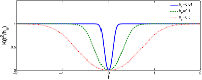
Figure 1: $K(\frac{t^{2}}{h_{n}})=\frac{\exp(t^{2}/h_{n})-1}{\exp(t^{2}/h_{n})+1}$ as an approximation to $I_{(t\neq 0)}$.

Smoothing the indicator function is often seen in the literature on high-dimensional variable selections. Recently, Bondell and Reich (2012) approximate $I_{(t\neq 0)}$ by $\frac{(h_{n}+1)t}{h_{n}+t}$ to obtain a tractable nonconvex optimization problem. Intuitively, we expect that the smoothed FGMM should also achieve the variable selection consistency. Indeed, the following theorem formally proves this claim.

Theorem 7.1

Suppose $h_{n}^{1-\gamma}=o(d_{n}^{2})$ for a small constant $\gamma\in(0,1)$. Under the assumptions of Theorem 4.1, there exists a local minimizer $\widehat{\bolds{\beta}}^{\prime}$ of the smoothed FGMM $Q_{K}(\bolds{\beta})$ such that, for $\widehat{S}^{\prime}=\{j\leq p\dvtx\widehat{\beta}_{j}^{\prime}\neq 0\}$,

$$P\bigl{(}\widehat{S}^{\prime}=S\bigr{)}\rightarrow 1.$$

In addition, the local minimizer $\widehat{\bolds{\beta}}^{\prime}$ is strict with probability at least $1-\delta$ for an arbitrarily small $\delta>0$ and all large $n$.

The asymptotic normality of the estimated nonzero coefficients can be established very similar to that of Theorem 4.1, which is omitted for brevity.

7.2 Coordinate descent algorithm

We employ the iterative coordinate algorithm for the smoothed FGMM minimization, which was used by Fu (1998), Daubechies, Defrise and De Mol (2004), Fan and Lv (2011), etc. The iterative coordinate algorithm minimizes one coordinate of $\bolds{\beta}$ at a time, with other coordinates kept fixed at their values obtained from previous steps, and successively updates each coordinate. The penalty function can be approximated by local linear approximation as in Zou and Li (2008).

Specifically, we run the regular penalized least squares to obtain an initial value, from which we start the iterative coordinate algorithm for the smoothed FGMM. Suppose $\bolds{\beta}^{(l)}$ is obtained at step $l$. For $k\in\{1,\ldots,p\}$, denote by $\bolds{\beta}^{(l)}_{(-k)}$ a $(p-1)$-dimensional vector consisting of all the components of $\bolds{\beta}^{(l)}$ but $\beta^{(l)}_{k}$. Write $(\bolds{\beta}^{(l)}_{(-k)},t)$ as the $p$-dimensional vector that replaces $\beta^{(l)}_{k}$ with $t$. The minimization with respect to $t$ while keeping $\bolds{\beta}^{(l)}_{(-k)}$ fixed is then a univariate minimization problem, which is not difficult to implement. To speed up the convergence, we can also use the second-order approximation of $L_{K}(\bolds{\beta}^{(l)}_{(-k)},t)$ along the $k$th component at $\beta_{k}^{(l)}$:

$$L_{K}\bigl{(}\bolds{\beta}^{(l)}_{(-k)},t\bigr{)}$$

$$\qquad\approx L_{K}\bigl{(}\bolds{\beta}^{(l)}\bigr{)}+\frac{\partial L_{K}(\bolds{\beta}^{(l)})}{\partial\beta_{k}}\bigl{(}t-\beta^{(l)}_{k}\bigr{)}+\frac{1}{2}\frac{\partial^{2}L_{K}(\bolds{\beta}^{(l)})}{\partial\beta_{k}^{2}}\bigl{(}t-\beta^{(l)}_{k}\bigr{)}^{2}$$ (22)

$$\qquad\equiv L_{K}\bigl{(}\bolds{\beta}^{(l)}\bigr{)}+\widehat{L}_{K}\bigl{(}\bolds{\beta}^{(l)}_{(-k)},t\bigr{)},$$

where $\widehat{L}_{K}(\bolds{\beta}^{(l)}_{(-k)},t)$ is a quadratic function of $t$. We solve for

$$t^{*}=\arg\min_{t}\widehat{L}_{K}\bigl{(}\bolds{\beta}^{(l)}_{(-k)},t\bigr{)}+P_{n}^{\prime}\bigl{(}\bigl{|}\beta^{(l)}_{k}\bigr{|}\bigr{)}|t|,$$ (23)

which admits an explicit analytical solution, and keep the remaining components at step $l$. Accept $t^{*}$ as an updated $k$th component of $\bolds{\beta}^{(l)}$ only if $L_{K}(\bolds{\beta}^{(l)})+\sum_{j=1}^{p}P_{n}(|\bolds{\beta}^{(l)}_{j}|)$ strictly decreases.

The coordinate descent algorithm runs as follows: [1.]

Set $l=1$. Initialize ${\bolds{\beta}}^{(1)}=\widehat{\bolds{\beta}}*$, where $\widehat{\bolds{\beta}}*$ solves

$$\min_{\bolds{\beta}\in\mathbb{R}^{p}}\frac{1}{n}\sum_{i=1}^{n}\bigl{[}g\bigl{(}Y_{i},\mathbf{X}_{i}^{T}\bolds{\beta}\bigr{)}\bigr{]}^{2}+\sum_{j=1}^{p}P_{n}\bigl{(}|\beta_{j}|\bigr{)}$$

using the coordinate descent algorithm as in Fan and Lv (2011).

Successively for $k=1,\ldots,p$, let $t^{*}$ be the minimizer of

$$\min_{t}\widehat{L}_{K}\bigl{(}\bolds{\beta}^{(l)}_{(-k)},t\bigr{)}+P_{n}^{\prime}\bigl{(}\bigl{|}\beta^{(l)}_{k}\bigr{|}\bigr{)}|t|.$$

Update ${\beta}^{(l)}_{k}$ as $t^{*}$ if

$$L_{K}\bigl{(}\bolds{\beta}^{(l)}_{(-k)},t^{*}\bigr{)}+P_{n}\bigl{(}\bigl{|}t^{*}\bigr{|}\bigr{)}<L_{K}\bigl{(}\bolds{\beta}^{(l)}\bigr{)}+P_{n}\bigl{(}\bigl{|}\beta^{(l)}_{k}\bigr{|}\bigr{)}.$$

Otherwise, set $\beta_{k}^{(l)}=\beta_{k}^{(l-1)}$. Increase $l$ by one when $k=p$.

Repeat step 2 until $|Q_{K}(\bolds{\beta}^{(l)})-Q_{K}(\bolds{\beta}^{(l+1)})|<\epsilon$, for a predetermined small $\epsilon$.

When the second-order approximation (7.2) is combined with SCAD in step 2, the local linear approximation of SCAD is not needed. As demonstrated in Fan and Li (2001), when $P_{n}(t)$ is defined using SCAD, the penalized optimization of the form $\min_{\beta\in\mathbb{R}}\frac{1}{2}(z-\beta)^{2}+\Lambda P_{n}(|\beta|)$ has an analytical solution.

We can show that the evaluated objective values $\{Q_{K}(\bolds{\beta}^{(l)})\}_{l\geq 1}$ is a bounded Cauchy sequence. Hence, for an arbitrarily small $\epsilon>0$, the above algorithm stops after finitely many steps. Let $M(\bolds{\beta})$ denote the map defined by the algorithm from $\bolds{\beta}^{(l)}$ to $\bolds{\beta}^{(l+1)}$. We define a stationary point of the function $Q_{K}(\bolds{\beta})$ to be any point $\bolds{\beta}$ at which the gradient vector of $Q_{K}(\bolds{\beta})$ is zero. Similar to the local linear approximation of Zou and Li (2008), we have the following result regarding the property of the algorithm.

Theorem 7.2

The sequence $\{Q_{K}(\bolds{\beta}^{(l)})\}_{l\geq 1}$ is a bounded nonincreasing Cauchy sequence. Hence, for any arbitrarily small $\epsilon>0$, the coordinate descent algorithm will stop after finitely many iterations. In addition, if $Q_{K}(\bolds{\beta})=Q_{K}(M(\bolds{\beta}))$ only for stationary points of $Q_{K}(\cdot)$ and if $\bolds{\beta}^{*}$ is a limit point of the sequence $\{\bolds{\beta}^{(l)}\}_{l\geq 1}$, then $\bolds{\beta}^{*}$ is a stationary point of $Q_{K}(\bolds{\beta})$.

Theoretical analysis of nonconvex regularization in the recent decade has focused on numerical procedures that can find local solutions [Hunter and Li (2005), Kim, Choi and Oh (2008), Brehenry and Huang (2011)]. Proving that the algorithm achieves a solution that possesses the desired oracle properties is technically difficult. Our simulated results demonstrate that the proposed algorithm indeed reaches the desired sparse estimator. Further investigation along the lines of Zhang and Zhang (2012) and Loh and Wainwright (2013) is needed to investigate the statistical properties of the solution to nonconvex optimization problems, which we leave as future research.

8 Monte Carlo experiments

8.1 Endogeneity in both important and unimportant regressors

To test the performance of FGMM for variable selection, we simulate from a linear model:

$$Y = \mathbf{X}^{T}\bolds{\beta}_{0}+\varepsilon,$$

$$(\beta_{01},\ldots,\beta_{05}) = (5,-4,7,-2,1.5),\qquad\beta_{0j}=0\qquad\mbox{for }6\leq j\leq p$$

with $p=50$ or $200$. Regressors are classified as being exogenous (independent of $\varepsilon$) and endogenous. For each component of $\mathbf{X}$, we write $X_{j}=X_{j}^{e}$ if $X_{j}$ is endogenous, and $X_{j}=X_{j}^{x}$ if $X_{j}$ is exogenous, and $X_{j}^{e}$ and $X_{j}^{x}$ are generated according to

$$X_{j}^{e}=(F_{j}+H_{j}+1)(3\varepsilon+1),\qquad X_{j}^{x}=F_{j}+H_{j}+u_{j},$$

where $\{\varepsilon,u_{1},\ldots,u_{p}\}$ are independent $N(0,1)$. Here $\mathbf{F}=(F_{1},\ldots,F_{p})^{T}$ and $\mathbf{H}=(H_{1},\ldots,H_{p})^{T}$ are the transformations (to be specified later) of a three-dimensional instrumental variable $\mathbf{W}=(W_{1},W_{2},W_{3})^{T}\sim N_{3}(0,I_{3})$. There are $m$ endogenous variables $(X_{1},X_{2},X_{3},X_{6},\ldots,X_{2+m})^{T}$, with $m=10$ or $50$. Hence, three of the important regressors $(X_{1},X_{2},X_{3})$ are endogenous while two are exogenous $(X_{4},X_{5})$.

We apply the Fourier basis as the working instruments:

$$\mathbf{F} = \sqrt{2}\bigl{\{}\sin(j\pi W_{1})+\sin(j\pi W_{2})+\sin(j\pi W_{3})\dvtx j\leq p\bigr{\}},$$

$$\mathbf{H} = \sqrt{2}\bigl{\{}\cos(j\pi W_{1})+\cos(j\pi W_{2})+\cos(j\pi W_{3})\dvtx j\leq p\bigr{\}}.$$

The data contain $n=100$ i.i.d. copies of $(Y,\mathbf{X},\mathbf{F},\mathbf{H})$. PLS and FGMM are carried out separately for comparison. In our simulation, we use SCAD with predetermined tuning parameters of $\lambda$ as the penalty function. The logistic cumulative distribution function with $h=0.1$ is used for smoothing:

$$F(t)=\frac{\exp(t)}{1+\exp(t)},\qquad K\biggl{(}\frac{\beta_{j}^{2}}{h}\biggr{)}=2F\biggl{(}\frac{\beta_{j}^{2}}{h}\biggr{)}-1.$$

There are 100 replications per experiment. Four performance measures are used to compare the methods. The first measure is the mean standard error (MSE_S) of the important regressors, determined by the average of $\|\widehat{\bolds{\beta}}_{S}-\bolds{\beta}_{0S}\|$ over the 100 replications, where $S=\{1,\ldots,5\}$. The second measure is the average of the MSE of unimportant regressors, denoted by MSE_N. The third measure is the number of correctly selected nonzero coefficients, that is, the true positive (TP), and finally, the fourth measure is the number of incorrectly selected coefficients, the false positive (FP). In addition, the standard error over the 100 replications of each measure is also reported. In each simulation, we initiate $\bolds{\beta}^{(0)}=(0,\ldots,0)^{T}$, and run a penalized least squares [SCAD($\lambda$)] for $\lambda=0.5$ to obtain the initial value for the FGMM procedure. The results of the simulation are summarized in Table 2, which compares the performance measures of PLS and FGMM.

Table 2: Endogeneity in both important and unimportant regressors, $n=100$

	PLS			FGMM
	$\bolds{\lambda=1}$	$\bolds{\lambda=3}$	$\bolds{\lambda=4}$	$\bolds{\lambda=0.08}$	$\bolds{\lambda=0.1}$	$\bolds{\lambda=0.3}$	post-FGMM
	$p=50$, $m=10$
MSES	0.190	0.525	0.491	0.106	0.097	0.102	0.088
	(0.102)	(0.283)	(0.328)	(0.051)	(0.043)	(0.037)	(0.026)
MSEN	0.171	0.240	0.183	0.090	0.085	0.048
	(0.059)	(0.149)	(0.149)	(0.030)	(0.035)	(0.034)
TP	5	5	4.97	5	5	5
	(0)	(0)	(0.171)	(0)	(0)	(0)
FP	27.69	14.63	10.37	3.76	3.5	1.63
	(6.260)	(5.251)	(4.539)	(1.093)	(1.193)	(1.070)
	$p=200$, $m=50$
MSES	0.831	0.966	1.107	0.111	0.104	0.231	0.092
	(0.787)	(0.595)	(0.678)	(0.048)	(0.041)	(0.431)	(0.032)
MSEN	1.286	0.936	0.828	0.062	0.063	0.053
	(1.333)	(0.799)	(0.656)	(0.018)	(0.021)	(0.075)
TP	5	4.9	4.73	5	5	4.94
	(0)	(0.333)	(0.468)	(0)	(0)	(0.246)
FP	86.760	42.440	35.070	4.726	4.276	2.897
	(27.41)	(15.08)	(13.84)	(1.358)	(1.251)	(2.093)

[]$m$ is the number of endogenous regressors. MSE_S is the average of $\|\widehat{\bolds{\beta}}_{S}-\bolds{\beta}_{0S}\|$ for nonzero coefficients. MSE_N is the average of $\|\widehat{\bolds{\beta}}_{N}-\bolds{\beta}_{0N}\|$ for zero coefficients. TP is the number of correctly selected variables; FP is the number of incorrectly selected variables, and $m$ is the total number of endogenous regressors. The standard error of each measure is also reported.

PLS has nonnegligible false positives (FP). The average FP decreases as the magnitude of the penalty parameter increases, however, with a relatively large MSE_S for the estimated nonzero coefficients, and the FP rate is still large compared to that of FGMM. The PLS also misses some important regressors for larger $\lambda$. It is worth noting that the larger MSE_S for PLS is due to the bias of the least squares estimation in the presence of endogeneity. In contrast, FGMM performs well in both selecting the important regressors, and in correctly eliminating the unimportant regressors. The average MSE_S of FGMM is significantly less than that of PLS since the instrumental variable estimation is applied instead. In addition, after the regressors are selected by the FGMM, the post-FGMM further reduces the mean squared error of the estimators.

8.2 Endogeneity only in unimportant regressors

Consider a similar linear model but only the unimportant regressors are endogenous and all the important regressors are exogenous, as designed in Section 2.2, so the true model is as the usual case without endogeneity. In this case, we apply $(\mathbf{F},\mathbf{H})=(\mathbf{X},\mathbf{X}^{2})$ as the working instruments for FGMM with SCAD$(\lambda)$ penalty, and need only data $\mathbf{X}$ and $\mathbf{Y}=(Y_{1},\ldots,Y_{n})$. We still compare the FGMM procedure with PLS. The results are reported in Table 3.

Table 3: Endogeneity only in unimportant regressors, $n=200$

	PLS			FGMM
	$\bolds{\lambda=0.1}$	$\bolds{\lambda=0.5}$	$\bolds{\lambda=1}$	$\bolds{\lambda=0.05}$	$\bolds{\lambda=0.1}$	$\bolds{\lambda=0.2}$
	$p=50$
MSES	0.133	0.629	1.417	0.261	0.184	0.194
	(0.043)	(0.301)	(0.329)	(0.094)	(0.069)	(0.076)
MSEN	0.068	0.072	0.095	0.001	0	0.001
	(0.016)	(0.016)	(0.019)	(0.010)	(0)	(0.009)
TP	5	4.82	3.63	5	5	5
	(0)	(0.385)	(0.504)	(0)	(0)	(0)
FP	35.36	8.84	2.58	0.08	0	0.02
	(3.045)	(3.334)	(1.557)	(0.337)	(0)	(0.141)
	$p=300$
MSES	0.159	0.650	1.430	0.274	0.187	0.193
	(0.054)	(0.304)	(0.310)	(0.086)	(0.102)	(0.123)
MSEN	0.107	0.071	0.086	$5\times 10^{-4}$	0	$5\times 10^{-4}$
	(0.019)	(0.023)	(0.027)	(0.006)	(0)	(0.005)
TP	5	4.82	3.62	5	5	4.99
	(0)	(0.384)	(0.487)	(0)	(0)	(0.100)
FP	210.47	42.78	7.94	0.11	0	0.01
	(11.38)	(11.773)	(5.635)	(0.37)	(0)	(0.10)

It is clearly seen that even though only the unimportant regressors are endogenous, however, the PLS still does not seem to select the true model correctly. This illustrates the variable selection inconsistency for PLS even when the true model has no endogeneity. In contrast, the penalized FGMM still performs relatively well.

8.3 Weak minimal signals

To study the effect on variable selection when the strength of the minimal signal is weak, we run another set of simulations with the same data generating process as in design 1 but we change $\beta_{4}=-0.5$ and $\beta_{5}=0.1$, and keep all the remaining parameters the same as before. The minimal nonzero signal becomes $|\beta_{5}|=0.1$. Three of the important regressors are endogenous as in design 1. Table 4 indicates that the minimal signal is so small that it is not easily distinguishable from the zero coefficients.

Table 4: FGMM for weak minimal signal $\bolds{\beta}_{4}=-0.5$, $\bolds{\beta}_{5}=0.1$

	$\bolds{p=50}$	$\bolds{m=10}$		$\bolds{p=200}$	$\bolds{m=50}$
	$\bolds{\lambda=0.05}$	$\bolds{\lambda=0.1}$	$\bolds{\lambda=0.5}$	$\bolds{\lambda=0.05}$	$\bolds{\lambda=0.1}$	$\bolds{\lambda=0.5}$
MSES	0.128	0.107	0.118	0.138	0.125	0.238
	(0.020)	(0.000)	(0.056)	(0.061)	(0.074)	(0.154)
MSEN	0.155	0.097	0.021	0.134	0.108	0.084
	(0.054)	(0.000)	(0.033)	(0.052)	(0.043)	(0.062)
TP	4.12	4	4	4.04	3.98	3.8
	(0.327)	(0)	(0)	(0.281)	(0.141)	(0.402)
FP	4.93	5	2.08	4.72	4.3	1.95
	(1.578)	(0)	(0.367)	(1.198)	(0.948)	(1.351)

9 Conclusion and discussion

Endogeneity can arise easily in the high-dimensional regression due to a large pool of regressors, which causes the inconsistency of the penalized least-squares methods and possible false scientific discoveries. Based on the over-identification assumption and valid instrumental variables, we propose to penalize an FGMM loss function. It is shown that FGMM possesses the oracle property, and the estimator is also a nearly global minimizer.

We would like to point out that this paper focuses on correctly specified sparse models, and the achieved results are “pointwise” for the true model. An important issue is the uniform inference where the sparse model may be locally misspecified. While the oracle property is of fundamental importance for high-dimensional methods in many scientific applications, it may not enable us to make valid inference about the coefficients uniformly across a large class of models [Leeb and Pötscher (2008), Belloni, Chernozhukov and Hansen (2014)]. Therefore, the “post-double-selection” method with imperfect model selection recently proposed by Belloni, Chernozhukov and Hansen (2014) is important for making uniform inference. Research along that line under high-dimensional endogeneity is important and we shall leave it for the future agenda.

Finally, as discussed in Bickel, Ritov and Tsybakov (2009) and van de Geer (2008), high-dimensional regression problems can be thought of as an approximation to a nonparametric regression problem with a “dictionary” of functions or growing number of sieves. Then in the presence of endogenous regressors, model (9) is closely related to the nonparametric conditional moment restricted model considered by, for example, Newey and Powell (2003), Ai and Chen (2003) and Chen and Pouzo (2012). While the penalization in the latter literature is similar to ours, it plays a different role and is introduced for different purposes. It will be interesting to find the underlying relationships between the two models.

Appendix A Proofs for Section 2

Throughout this Appendix, $C$ will denote a generic positive constant that may be different in different uses. Let $\operatorname{sgn}(\cdot)$ denote the sign function.

A.1 Proof of Theorem 2.1

When $\widehat{\bolds{\beta}}$ is a local minimizer of $Q_{n}(\bolds{\beta})$, by the Karush–Kuhn–Tucker (KKT) condition, $\forall l\leq p$,

$$\frac{\partial L_{n}(\widehat{\bolds{\beta}})}{\partial\beta_{l}}+v_{l}=0,$$

where $v_{l}=P_{n}^{\prime}(|\widehat{\beta}_{l}|)\operatorname{sgn}(\widehat{\beta}_{l})$ if $\widehat{\beta}_{l}\neq 0$; $v_{l}\in[-P_{n}^{\prime}(0^{+}),P_{n}^{\prime}(0^{+})]$ if $\widehat{\beta}_{l}=0$, and we denote $P_{n}^{\prime}(0^{+})=\lim_{t\rightarrow 0^{+}}P_{n}^{\prime}(t)$. By the monotonicity of $P_{n}^{\prime}(t)$, we have $|\partial L_{n}(\widehat{\bolds{\beta}})/\partial\beta_{l}|\leq P_{n}^{\prime}(0^{+})$. By the Taylor expansion and the Cauchy–Schwarz inequality, there is $\tilde{\bolds{\beta}}$ on the segment joining $\widehat{\bolds{\beta}}$ and $\bolds{\beta}_{0}$ so that, on the event $\widehat{\bolds{\beta}}_{N}=0$, ($\widehat{\beta}_{j}-\beta_{0j}=0$ for all $j\notin S$)

$$\biggl{|}\frac{\partial L_{n}(\widehat{\bolds{\beta}})}{\partial\beta_{l}}-\frac{\partial L_{n}({\bolds{\beta}_{0}})}{\partial\beta_{l}}\biggr{|}=\Biggl{|}\sum_{j=1}^{p}\frac{\partial^{2}L_{n}(\tilde{\bolds{\beta}})}{\partial\beta_{l}\,\partial\beta_{j}}(\widehat{\beta}_{j}-\beta_{0j})\Biggr{|}=\biggl{|}\sum_{j\in S}\frac{\partial^{2}L_{n}(\tilde{\bolds{\beta}})}{\partial\beta_{l}\,\partial\beta_{j}}(\widehat{\beta}_{j}-\beta_{0j})\biggr{|}.$$

The Cauchy–Schwarz inequality then implies that $\max_{l\leq p}|\partial L_{n}(\widehat{\bolds{\beta}})/\partial\beta_{l}-\partial L_{n}({\bolds{\beta}_{0}})/\partial\beta_{l}|$ is bounded by

$$\max_{l,j\leq p}\biggl{|}\frac{\partial^{2}L_{n}(\tilde{\bolds{\beta}})}{\partial\beta_{l}\,\partial\beta_{j}}\biggr{|}\|\widehat{\bolds{\beta}}_{S}-\bolds{\beta}_{0S}\|_{1}\leq\max_{l,j\leq p}\biggl{|}\frac{\partial^{2}L_{n}(\tilde{\bolds{\beta}})}{\partial\beta_{l}\,\partial\beta_{j}}\biggr{|}\sqrt{s}\|\widehat{\bolds{\beta}}_{S}-\bolds{\beta}_{0S}\|.$$

By our assumption, $\sqrt{s}\|\widehat{\bolds{\beta}}_{S}-\bolds{\beta}_{0S}\|=o_{p}(1)$. Because $P(\widehat{\bolds{\beta}}_{N}=0)\rightarrow 1$,

$$\max_{l\leq p}\biggl{|}\frac{\partial L_{n}(\widehat{\bolds{\beta}})}{\partial\beta_{l}}-\frac{\partial L_{n}({\bolds{\beta}_{0}})}{\partial\beta_{l}}\biggr{|}\to^{p}0.$$ (24)

This yields that $\partial L_{n}({\bolds{\beta}_{0}})/\partial\beta_{l}=o_{p}(1)$.

A.2 Proof of Theorem 2.2

Let $\{X_{il}\}_{i=1}^{n}$ be the i.i.d. data of $X_{l}$ where $X_{l}$ is an endogenous regressor. For the penalized LS, $L_{n}(\bolds{\beta})=\frac{1}{n}\sum_{i=1}^{n}(Y_{i}-\mathbf{X}_{i}^{T}\bolds{\beta})^{2}$. Under the theorem assumptions, by the strong law of large number $\partial_{\beta_{l}}L_{n}(\bolds{\beta}_{0})=-\frac{2}{n}\sum_{i=1}^{n}X_{il}(Y_{i}-\mathbf{X}_{i}^{T}\bolds{\beta}_{0})\rightarrow-2E(X_{l}\varepsilon)$ almost surely, which does not satisfy (7) of Theorem 2.1.

Appendix B General penalized regressions

We present some general results for the oracle properties of penalized regressions. These results will be employed to prove the oracle properties for the proposed FGMM. Consider a penalized regression of the form:

$$\min_{\bolds{\beta}\in\mathbb{R}^{p}}L_{n}(\bolds{\beta})+\sum_{j=1}^{p}P_{n}\bigl{(}|\beta_{j}|\bigr{)},$$

Lemma B.1.

Under Assumption 4.1, if $\bolds{\beta}=(\beta_{1},\ldots,\beta_{s})^{T}$ is such that $\max_{j\leq s}|\beta_{j}-\beta_{0S,j}|\leq d_{n}$, then

$$\Biggl{|}\sum_{j=1}^{s}P_{n}\bigl{(}|\beta_{j}|\bigr{)}-P_{n}\bigl{(}|\beta_{0S,j}|\bigr{)}\Biggr{|}\leq\|\bolds{\beta}-\bolds{\beta}_{0S}\|\sqrt{s}P_{n}^{\prime}(d_{n}).$$

By Taylor’s expansion, there exists $\bolds{\beta}^{*}$ ($\bolds{\beta}_{j}^{*}\neq 0$ for each $j$) lying on the line segment joining $\bolds{\beta}$ and $\bolds{\beta}_{0S}$, such that

$$\sum_{j=1}^{s}\bigl{(}P_{n}\bigl{(}|\beta_{j}|\bigr{)}-P_{n}\bigl{(}|\beta_{0S,j}|\bigr{)}\bigr{)}$$

$$\qquad=\bigl{(}P_{n}^{\prime}\bigl{(}\bigl{|}\beta_{1}^{*}\bigr{|}\bigr{)}\operatorname{sgn}\bigl{(}\beta_{1}^{*}\bigr{)},\ldots,P_{n}^{\prime}\bigl{(}\bigl{|}\beta_{s}^{*}\bigr{|}\bigr{)}\operatorname{sgn}\bigl{(}\beta_{s}^{*}\bigr{)}\bigr{)}^{T}(\bolds{\beta}-\bolds{\beta}_{0S})$$

$$\qquad\leq\|\bolds{\beta}-\bolds{\beta}_{0S}\|\sqrt{s}\max_{j\leq s}P_{n}^{\prime}\bigl{(}\bigl{|}\beta^{*}_{j}\bigr{|}\bigr{)}.$$

Then $\min\{|\beta^{*}_{j}|\dvtx j\leq s\}\geq\min\{|\beta_{0S,j}|\dvtx j\leq s\}-\max_{j\leq s}|\beta^{*}_{j}-\beta_{0S,j}|$ $\geq 2d_{n}-d_{n}=d_{n}$.

Since $P_{n}^{\prime}$ is nonincreasing (as $P_{n}$ is concave), $P_{n}^{\prime}(|\beta^{*}_{j}|)\leq P_{n}^{\prime}(d_{n})$ for all $j\leq s$. Therefore $\sum_{j=1}^{s}(P_{n}(|\beta_{j}|)-P_{n}(|\beta_{0S,j}|)\leq\|\bolds{\beta}-\bolds{\beta}_{0S}\|\sqrt{s}P_{n}^{\prime}(d_{n})$.

In the theorems below, with $S=\{j\dvtx\beta_{0j}\neq 0\}$, define a so-called “oracle space” $\mathcal{B}=\{\bolds{\beta}\in\mathbb{R}^{p}\dvtx\beta_{j}=0\mbox{ if }j\notin S\}$. Write $L_{n}(\bolds{\beta}_{S},0)=L_{n}(\bolds{\beta})$ for $\bolds{\beta}=(\bolds{\beta}_{S}^{T},0)^{T}\in\mathcal{B}$. Let $\bolds{\beta}_{S}=(\beta_{S1},\ldots,\beta_{Ss})$ and

$$\nabla_{S}L_{n}(\bolds{\beta}_{S},0)=\biggl{(}\frac{\partial L_{n}(\bolds{\beta}_{S},0)}{\partial\beta_{S1}},\ldots,\frac{\partial L_{n}(\bolds{\beta}_{S},0)}{\partial\beta_{Ss}}\biggr{)}^{T}.$$

Theorem B.1 ((Oracle consistency))

Suppose Assumption 4.1 holds. In addition, suppose $L_{n}(\bolds{\beta}_{S},0)$ is twice differentiable with respect to $\bolds{\beta}_{S}$ in a neighborhood of $\bolds{\beta}_{0S}$ restricted on the subspace $\mathcal{B}$, and there exists a positive sequence $a_{n}=o(d_{n})$ such that

$$\hskip 13.0pt\mathrm{(i)}\hskip 103.0pt\qquad\bigl{\|}\nabla_{S}L_{n}(\bolds{\beta}_{0S},0)\bigr{\|}=O_{p}(a_{n}).$$

(ii) For any $\epsilon>0$, there is $C_{\epsilon}>0$ so that for all large $n$,

$$P\bigl{(}\lambda_{\min}\bigl{(}\nabla_{S}^{2}L_{n}(\bolds{\beta}_{0S},0)\bigr{)}>C_{\epsilon}\bigr{)}>1-\epsilon.$$ (25)

(iii) For any $\epsilon>0,\delta>0$, and any nonnegative sequence $\alpha_{n}=o(d_{n})$, there is $N>0$ such that when $n>N$,

$$P\Bigl{(}\sup_{\|\beta_{S}-\beta_{0S}\|\leq\alpha_{n}}\bigl{\|}\nabla_{S}^{2}L_{n}(\bolds{\beta}_{S},0)-\nabla_{S}^{2}L_{n}(\bolds{\beta}_{0S},0)\bigr{\|}_{F}\leq\delta\Bigr{)}>1-\epsilon.$$ (26)

Then there exists a local minimizer $\widehat{\bolds{\beta}}=(\widehat{\bolds{\beta}}{}^{T}_{S},0)^{T}$ of

$$Q_{n}(\bolds{\beta}_{S},0)=L_{n}(\bolds{\beta}_{S},0)+\sum_{j\in S}P_{n}\bigl{(}|\beta_{j}|\bigr{)}$$

such that $\|\widehat{\bolds{\beta}}_{S}-\bolds{\beta}_{0S}\|=O_{p}(a_{n}+\sqrt{s}P_{n}^{\prime}(d_{n}))$. In addition, for an arbitrarily small $\epsilon>0$, the local minimizer $\widehat{\bolds{\beta}}$ is strict with probability at least $1-\epsilon$, for all large $n$.

The proof is a generalization of the proof of Theorem 3 in Fan and Lv (2011). Let $k_{n}=a_{n}+\sqrt{s}P_{n}^{\prime}(d_{n})$. It is our assumption that $k_{n}=o(1)$. Write $Q_{1}(\bolds{\beta}_{S})=Q_{n}(\bolds{\beta}_{S},0)$, and $L_{1}(\bolds{\beta}_{S})=L_{n}(\bolds{\beta}_{S},0)$. In addition, write

$$\nabla L_{1}(\bolds{\beta}_{S})=\frac{\partial L_{n}}{\partial\bolds{\beta}_{S}}(\bolds{\beta}_{S},0)\quad\mbox{and}\quad\nabla^{2}L_{1}(\bolds{\beta}_{S})=\frac{\partial^{2}L_{n}}{\partial\bolds{\beta}_{S}\bolds{\beta}_{S}^{T}}(\bolds{\beta}_{S},0).$$

Define $\mathcal{N}_{\tau}=\{\bolds{\beta}\in\mathbb{R}^{s}\dvtx\|\bolds{\beta}-\bolds{\beta}_{0S}\|\leq k_{n}\tau\}$ for some $\tau>0$. Let $\partial\mathcal{N}_{\tau}$ denote the boundary of $\mathcal{N}_{\tau}$. Now define an event

$$H_{n}(\tau)=\Bigl{\{}Q_{1}(\bolds{\beta}_{0S})<\min_{\bolds{\beta}_{S}\in\partial\mathcal{N}_{\tau}}Q_{1}(\bolds{\beta}_{S})\Bigr{\}}.$$

On the event $H_{n}(\tau)$, by the continuity of $Q_{1}$, there exists a local minimizer of $Q_{1}$ inside $\mathcal{N}_{\tau}$. Equivalently, there exists a local minimizer $(\widehat{\bolds{\beta}}{}^{T}_{S},0)^{T}$ of $Q_{n}$ restricted on $\mathcal{B}=\{\bolds{\beta}=(\bolds{\beta}_{S}^{T},0)^{T}\}$ inside $\{\bolds{\beta}=(\bolds{\beta}_{S}^{T},0)^{T}\dvtx\bolds{\beta}_{S}\in\mathcal{N}_{\tau}\}$. Therefore, it suffices to show that $\forall\epsilon>0$, there exists $\tau>0$ so that $P(H_{n}(\tau))>1-\epsilon$ for all large $n$, and that the local minimizer is strict with probability arbitrarily close to one.

For any $\bolds{\beta}_{S}\in\partial\mathcal{N}_{\tau}$, which is $\|\bolds{\beta}_{S}-\bolds{\beta}_{0S}\|=k_{n}\tau$, there is $\bolds{\beta}^{*}$ lying on the segment joining $\bolds{\beta}_{S}$ and $\bolds{\beta}_{0S}$ such that by Taylor’s expansion on $L_{1}(\bolds{\beta}_{S})$:

$$Q_{1}(\bolds{\beta}_{S})-Q_{1}(\bolds{\beta}_{0S}) = (\bolds{\beta}_{S}-\bolds{\beta}_{0S})^{T}\nabla L_{1}(\bolds{\beta}_{0S})$$

$${}+\frac{1}{2}(\bolds{\beta}_{S}-\bolds{\beta}_{0S})^{T}\nabla^{2}L_{1}\bigl{(}\bolds{\beta}^{*}\bigr{)}(\bolds{\beta}_{S}-\bolds{\beta}_{0S})$$

$${}+\sum_{j=1}^{s}\bigl{[}P_{n}\bigl{(}|\beta_{Sj}|\bigr{)}-P_{n}\bigl{(}|\beta_{0S,j}|\bigr{)}\bigr{]}.$$

By condition (i) $\|\nabla L_{1}(\bolds{\beta}_{0S})\|=O_{p}(a_{n})$, for any $\epsilon>0$, there exists $C_{1}>0$, so that the event $H_{1}$ satisfies $P(H_{1})>1-\epsilon/4$ for all large $n$, where

$$H_{1}=\bigl{\{}(\bolds{\beta}_{S}-\bolds{\beta}_{0S})^{T}\nabla L_{1}(\bolds{\beta}_{0S})\geq-C_{1}\|\bolds{\beta}_{S}-\bolds{\beta}_{0S}\|a_{n}\bigr{\}}.$$ (27)

In addition, condition (ii) yields that there exists $C_{\epsilon}>0$ such that the following event $H_{2}$ satisfies $P(H_{2})\geq 1-\epsilon/4$ for all large $n$, where

$$H_{2}=\bigl{\{}(\bolds{\beta}_{S}-\bolds{\beta}_{0S})^{T}\nabla^{2}L_{1}(\bolds{\beta}_{0S})(\bolds{\beta}_{S}-\bolds{\beta}_{0S})>C_{\epsilon}\|\bolds{\beta}_{S}-\bolds{\beta}_{0S}\|^{2}\bigr{\}}.$$ (28)

Define another event $H_{3}=\{\|\nabla^{2}L_{1}(\bolds{\beta}_{0S})-\nabla^{2}L_{1}(\bolds{\beta}^{*})\|_{F}<C_{\epsilon}/4\}$. Since $\|\bolds{\beta}_{S}-\bolds{\beta}_{0S}\|=k_{n}\tau$, by condition (26) for any $\tau>0$, $P(H_{3})>1-\epsilon/4$ for all large $n$. On the event $H_{2}\cap H_{3}$, the following event $H_{4}$ holds:

$$H_{4}=\biggl{\{}(\bolds{\beta}_{S}-\bolds{\beta}_{0S})^{T}\nabla^{2}L_{1}\bigl{(}\bolds{\beta}^{*}\bigr{)}(\bolds{\beta}_{S}-\bolds{\beta}_{0S})>\frac{3C_{\epsilon}}{4}\|\bolds{\beta}_{S}-\bolds{\beta}_{0S}\|^{2}\biggr{\}}.$$

By Lemma B.1, $\sum_{j=1}^{s}[P_{n}(|\beta_{Sj}|)-P_{n}(|\beta_{0S,j}|)]\geq-\sqrt{s}P_{n}^{\prime}(d_{n})\|\bolds{\beta}_{S}-\bolds{\beta}_{0S}\|$. Hence, for any $\bolds{\beta}_{S}\in\partial\mathcal{N}_{\tau}$, on $H_{1}\cap H_{4}$,

$$Q_{1}(\bolds{\beta}_{S})-Q_{1}(\bolds{\beta}_{0S})\geq k_{n}\tau\biggl{(}\frac{3k_{n}\tau C_{\epsilon}}{8}-C_{1}a_{n}-\sqrt{s}P_{n}^{\prime}(d_{n})\biggr{)}.$$

For $k_{n}=a_{n}+\sqrt{s}P_{n}^{\prime}(d_{n})$, we have $C_{1}a_{n}+\sqrt{s}P_{n}^{\prime}(d_{n})\leq(C_{1}+1)k_{n}$. Therefore, we can choose $\tau>8(C_{1}+1)/(3C_{\epsilon})$ so that $Q_{1}(\bolds{\beta}_{S})-Q_{1}(\bolds{\beta}_{0S})\geq 0$ uniformly for $\bolds{\beta}\in\partial\mathcal{N}_{\tau}$. Thus, for all large $n$, when $\tau>8(C_{1}+1)/(3C_{\epsilon})$,

$$P\bigl{(}H_{n}(\tau)\bigr{)}\geq P(H_{1}\cap H_{4})\geq 1-\epsilon.$$

It remains to show that the local minimizer in $\mathcal{N}_{\tau}$ (denoted by $\widehat{\bolds{\beta}}_{S}$) is strict with a probability arbitrarily close to one. For each $h\in\mathbb{R}/\{0\}$, define

$$\psi(h)=\limsup_{\epsilon\rightarrow 0^{+}}\mathop{\sup_{t_{1}<t_{2}}}_{(t_{1},t_{2})\in(|h|-\epsilon,|h|+\epsilon)}-\frac{P_{n}^{\prime}(t_{2})-P_{n}^{\prime}(t_{1})}{t_{2}-t_{1}}.$$

By the concavity of $P_{n}(\cdot)$, $\psi(\cdot)\geq 0$. We know that $L_{1}$ is twice differentiable on $\mathbb{R}^{s}$. For $\bolds{\beta}_{S}\in\mathcal{N}_{\tau}$. Let $\mathbf{A}(\bolds{\beta}_{S})=\nabla^{2}L_{1}(\bolds{\beta}_{S})-\operatorname{diag}\{\psi(\beta_{S1}),\ldots,\psi(\beta_{Ss})\}$. It suffices to show that $\mathbf{A}(\widehat{\bolds{\beta}}_{S})$ is positive definite with probability arbitrarily close to one. On the event $H_{5}=\{\eta(\widehat{\bolds{\beta}}_{S})\leq\sup_{\beta\in B(\beta_{0S},cd_{n})}\eta(\bolds{\beta})\}$ [where $cd_{n}$ is as defined in Assumption 4.1(iv)],

$$\max_{j\leq s}\psi(\widehat{\beta}_{S,j})\leq\eta(\widehat{\bolds{\beta}}_{S})\leq\sup_{\beta\in B(\beta_{0S},cd_{n})}\eta(\bolds{\beta}).$$

Also, define events $H_{6}=\{\|\nabla^{2}L_{1}(\widehat{\bolds{\beta}}_{S})-\nabla^{2}L_{1}(\bolds{\beta}_{0S})\|_{F}<C_{\epsilon}/4\}$ and $H_{7}=\{\lambda_{\min}(\nabla^{2}L_{1}(\bolds{\beta}_{0S}))>C_{\epsilon}\}$. Then on $H_{5}\cap H_{6}\cap H_{7}$, for any $\bolds{\alpha}\in\mathbb{R}^{s}$ satisfying $\|\bolds{\alpha}\|=1$, by Assumption 4.1(iv),

$$\bolds{\alpha}^{T}\mathbf{A}(\widehat{\bolds{\beta}}_{S})\bolds{\alpha} \geq \bolds{\alpha}^{T}\nabla^{2}L_{1}(\bolds{\beta}_{0S})\bolds{\alpha}-\bigl{|}\bolds{\alpha}^{T}\bigl{(}\nabla^{2}L_{1}(\widehat{\bolds{\beta}}_{S})-\nabla^{2}L_{1}(\bolds{\beta}_{0S})\bigr{)}\bolds{\alpha}\bigr{|}-\max_{j\leq s}\psi(\widehat{\beta}_{S,j})$$

$$\geq 3C_{\epsilon}/4-\sup_{\beta\in B(\beta_{0S},d_{n})}\eta(\bolds{\beta})\geq C_{\epsilon}/4$$

for all large $n$. This then implies $\lambda_{\min}(\mathbf{A}(\widehat{\bolds{\beta}}_{S}))\geq C_{\epsilon}/4$ for all large $n$.

We know that $P(\lambda_{\min}[\nabla^{2}L_{1}(\bolds{\beta}_{0S})]>C_{\epsilon})>1-\epsilon$. It remains to show that $P(H_{5}\cap H_{6})>1-\epsilon$ for arbitrarily small $\epsilon$. Because $k_{n}=o(d_{n})$, for an arbitrarily small $\epsilon>0$, $P(H_{5})\geq P(\widehat{\bolds{\beta}}_{S}\in B(\bolds{\beta}_{0S},cd_{n}))\geq 1-\epsilon/2$ for all large $n$. Finally,

$$P\bigl{(}H_{6}^{c}\bigr{)} \leq P\bigl{(}H_{6}^{c},\|\widehat{\bolds{\beta}}_{S}-\bolds{\beta}_{0S}\|\leq k_{n}\bigr{)}+P\bigl{(}\|\widehat{\bolds{\beta}}_{S}-\bolds{\beta}_{0S}\|>k_{n}\bigr{)}$$

$$\leq P\Bigl{(}\sup_{\|\beta_{S}-\beta_{0S}\|\leq k_{n}}\bigl{\|}\nabla^{2}L_{1}(\bolds{\beta}_{S})-\nabla^{2}L_{1}(\bolds{\beta}_{0S})\bigr{\|}_{F}\geq C_{\epsilon}/4\Bigr{)}+\epsilon/4$$

$$= \epsilon/2.$$

The previous theorem assumes that the true support $S$ is known, which is not practical. We therefore need to derive the conditions under which $S$ can be recovered from the data with probability approaching one. This can be done by demonstrating that the local minimizer of $Q_{n}$ restricted on $\mathcal{B}$ is also a local minimizer on $\mathbb{R}^{p}$. The following theorem establishes the variable selection consistency of the estimator, defined as a local solution to a penalized regression problem on $\mathbb{R}^{p}$.

For any $\bolds{\beta}\in\mathbb{R}^{p}$, define the projection function

$$\mathbb{T}\bolds{\beta}=\bigl{(}\beta_{1}^{\prime},\beta_{2}^{\prime},\ldots,\beta_{p}^{\prime}\bigr{)}^{T}\in\mathcal{B},\qquad\beta_{j}^{\prime}=\cases{\beta_{j},&\quad$\mbox{if }j\in S,$\vspace*{2pt}\cr 0,&\quad$\mbox{if }j\notin S.$}$$ (29)

Theorem B.2 ((Variable selection))

Suppose $L_{n}\dvtx\mathbb{R}^{p}\rightarrow\mathbb{R}$ satisfies the conditions in Theorem B.1, and Assumption 4.1 holds. Assume the following condition A holds.

Condition A: With probability approaching one, for $\widehat{\bolds{\beta}}_{S}$ in Theorem B.1, there exists a neighborhood $\mathcal{H}\subset\mathbb{R}^{p}$ of $(\widehat{\bolds{\beta}}{}^{T}_{S},0)^{T}$, such that for all $\bolds{\beta}=(\bolds{\beta}_{S}^{T},\break\bolds{\beta}_{N}^{T})^{T}\in\mathcal{H}$ but $\bolds{\beta}_{N}\neq 0$,

$$L_{n}(\mathbb{T}\bolds{\beta})-L_{n}(\bolds{\beta})<\sum_{j\notin S}P_{n}\bigl{(}|\beta_{j}|\bigr{)}.$$ (30)

Then (i) with probability approaching one, $\widehat{\bolds{\beta}}=(\widehat{\bolds{\beta}}{}^{T}_{S},0)^{T}$ is a local minimizer in $\mathbb{R}^{p}$ of

$$Q_{n}(\bolds{\beta})=L_{n}(\bolds{\beta})+\sum_{i=1}^{p}P_{n}\bigl{(}|\beta_{i}|\bigr{)}.$$

(ii) For an arbitrarily small $\epsilon>0$, the local minimizer $\widehat{\bolds{\beta}}$ is strict with probability at least $1-\epsilon$, for all large $n$.

Let $\widehat{\bolds{\beta}}=(\widehat{\bolds{\beta}}{}^{T}_{S},0)^{T}$ with $\widehat{\bolds{\beta}}_{S}$ being the local minimizer of $Q_{1}(\bolds{\beta}_{S})$ as in Theorem B.1. We now show: with probability approaching one, there is a random neighborhood of $\widehat{\bolds{\beta}}$, denoted by $\mathcal{H}$, so that $\forall\bolds{\beta}=(\bolds{\beta}_{S},\bolds{\beta}_{N})\in\mathcal{H}$ with $\bolds{\beta}_{N}\neq 0$, we have $Q_{n}(\widehat{\bolds{\beta}})<Q_{n}(\bolds{\beta})$. The last inequality is strict.

To show this, first note that we can take $\mathcal{H}$ sufficiently small so that $Q_{1}(\widehat{\bolds{\beta}}_{S})\leq Q_{1}(\bolds{\beta}_{S})$ because $\widehat{\bolds{\beta}}_{S}$ is a local minimizer of $Q_{1}(\bolds{\beta}_{S})$ from Theorem B.1. Recall the projection defined to be $\mathbb{T}\bolds{\beta}=(\bolds{\beta}_{S}^{T},0)^{T}$, and $Q_{n}(\mathbb{T}\bolds{\beta})=Q_{1}(\bolds{\beta}_{S})$ by the definition of $Q_{1}$. We have $Q_{n}(\widehat{\bolds{\beta}})=Q_{1}(\widehat{\bolds{\beta}}_{S})\leq Q_{1}(\bolds{\beta}_{S})=Q_{n}(\mathbb{T}\bolds{\beta})$. Therefore, it suffices to show that with probability approaching one, there is a sufficiently small neighborhood of $\mathcal{H}$ of $\widehat{\bolds{\beta}}$, so that for any $\bolds{\beta}=(\bolds{\beta}_{S}^{T},\bolds{\beta}_{N}^{T})^{T}\in\mathcal{H}$ with $\bolds{\beta}_{N}\neq 0$, $Q_{n}(\mathbb{T}\bolds{\beta})<Q_{n}(\bolds{\beta})$.

In fact, this is implied by condition (30):

$$Q_{n}(\mathbb{T}\bolds{\beta})-Q_{n}(\bolds{\beta})$$

(31)

$$\qquad=L_{n}(\mathbb{T}\bolds{\beta})-L_{n}(\bolds{\beta})-\Biggl{(}\sum_{j=1}^{p}P_{n}(\beta_{j})-\sum_{j=1}^{s}P_{n}\bigl{(}\bigl{|}(\mathbb{T}\bolds{\beta})_{j}\bigr{|}\bigr{)}\Biggr{)}<0.$$

The above inequality, together with the last statement of Theorem B.1 implies part (ii) of the theorem.

Appendix C Proofs for Section 4

Throughout the proof, we write $\mathbf{F}_{iS}=\mathbf{F}_{i}(\bolds{\beta}_{0S})$, $\mathbf{H}_{iS}=\mathbf{H}_{i}(\bolds{\beta}_{0S})$ and $\mathbf{V}_{iS}=(\mathbf{F}_{iS}^{T},\mathbf{H}^{T}_{iS})^{T}$.

Lemma C.1.

(i) $\max_{l\leq p}|\frac{1}{n}\sum_{i=1}^{n}(F_{ij}-\bar{F}_{j})^{2}-\operatorname{var}(F_{j})|=o_{p}(1)$. [(iii)]

$\max_{l\leq p}|\frac{1}{n}\sum_{i=1}^{n}(H_{ij}-\bar{H}_{j})^{2}-\operatorname{var}(H_{j})|=o_{p}(1)$.

$\sup_{\bolds{\beta}\in\mathbb{R}^{p}}\lambda_{\max}(\mathbf{J}(\bolds{\beta}))=O_{p}(1)$, and $\lambda_{\min}(\mathbf{J}(\bolds{\beta}_{0}))$ is bounded away from zero with probability approaching one.

Parts (i) and (ii) follow from an application of the standard large deviation theory by using Bernstein inequality and Bonferroni’s method. Part (iii) follows from the assumption that $\operatorname{var}(F_{j})$ and $\operatorname{var}(H_{j})$ are bounded uniformly in $j\leq p$.

C.1 Verifying conditions in Theorems B.1, B.2

C.1.1 Verifying conditions in Theorem B.1

For any $\bolds{\beta}\in\mathbb{R}^{p}$, we can write $\mathbb{T}\bolds{\beta}=(\bolds{\beta}_{S}^{T},0)^{T}$. Define

$$\tilde{L}_{\mathrm{FGMM}}(\bolds{\beta}_{S})=\Biggl{[}\frac{1}{n}\sum_{i=1}^{n}g\bigl{(}Y_{i},\mathbf{X}_{iS}^{T}\bolds{\beta}_{S}\bigr{)}\mathbf{V}_{iS}\Biggr{]}^{T}\mathbf{J}(\bolds{\beta}_{0})\Biggl{[}\frac{1}{n}\sum_{i=1}^{n}g\bigl{(}Y_{i},\mathbf{X}_{iS}^{T}\bolds{\beta}_{S}\bigr{)}\mathbf{V}_{iS}\Biggr{]}.$$

Then $\tilde{L}_{\mathrm{FGMM}}(\bolds{\beta}_{S})=L_{\mathrm{FGMM}}(\bolds{\beta}_{S},0)$.

Condition (i): $\nabla\tilde{L}_{\mathrm{FGMM}}(\bolds{\beta}_{0S})=2\mathbf{A}_{n}(\bolds{\beta}_{0S})\mathbf{J}(\bolds{\beta}_{0})[\frac{1}{n}\sum_{i=1}^{n}g(Y_{i},\mathbf{X}_{iS}^{T}\bolds{\beta}_{0S})\mathbf{V}_{iS}]$, where

$$\mathbf{A}_{n}(\bolds{\beta}_{S})\equiv\frac{1}{n}\sum_{i=1}^{n}m\bigl{(}Y_{i},\mathbf{X}_{iS}^{T}\bolds{\beta}_{S}\bigr{)}\mathbf{X}_{iS}\mathbf{V}_{iS}^{T}.$$ (32)

By Assumption 4.5, $\|\mathbf{A}_{n}(\bolds{\beta}_{0})\|=O_{p}(1)$. In addition, the elements in $\mathbf{J}(\bolds{\beta}_{0})$ are uniformly bounded in probability due to Lemma C.1. Hence,$\|\nabla\tilde{L}_{\mathrm{FGMM}}(\bolds{\beta}_{0S})\|\leq O_{p}(1)\|\frac{1}{n}\sum_{i=1}^{n}g(Y_{i},\mathbf{X}_{iS}^{T}\bolds{\beta}_{0S})\mathbf{V}_{iS}\|$. Due to $Eg(Y,\break\mathbf{X}_{S}^{T}\bolds{\beta}_{0S})\mathbf{V}_{S}=0$, using the exponential-tail Bernstein inequality with Assumption 4.3 plus Bonferroni inequality, it can be shown that there is $C>0$ such that for any $t>0$,

$$P\Biggl{(}\max_{l\leq p}\biggl{|}\frac{1}{n}\sum_{i=1}^{n}g\bigl{(}Y_{i},\mathbf{X}_{iS}^{T}\bolds{\beta}_{0S}\bigr{)}F_{li}\biggr{|}>t\Biggr{)}$$

$$\qquad<p\max_{l\leq p}P\Biggl{(}\biggl{|}\frac{1}{n}\sum_{i=1}^{n}g\bigl{(}Y_{i},\mathbf{X}_{iS}^{T}\bolds{\beta}_{0S}\bigr{)}F_{li}\biggr{|}>t\Biggr{)}\leq\exp\bigl{(}\log p-Ct^{2}/n\bigr{)},$$

which implies $\max_{l\leq p}|\frac{1}{n}\sum_{i=1}^{n}g(Y_{i},\mathbf{X}_{iS}^{T}\bolds{\beta}_{0S})F_{li}|=O_{p}(\sqrt{\frac{\log p}{n}})$. Similarly,$\max_{l\leq p}|\frac{1}{n}\sum_{i=1}^{n}g(Y_{i},\mathbf{X}_{iS}^{T}\bolds{\beta}_{0S})H_{li}|=O_{p}(\sqrt{\frac{\log p}{n}})$. Hence $\|\nabla\tilde{L}_{\mathrm{FGMM}}(\bolds{\beta}_{0S})\|=O_{p}(\sqrt{(s\log p)/n})$.

Condition (ii): Straightforward but tedious calculation yields

$$\nabla^{2}\tilde{L}_{\mathrm{FGMM}}(\bolds{\beta}_{0S})=\bolds{\Sigma}(\bolds{\beta}_{0S})+\mathbf{M}(\bolds{\beta}_{0S}),$$

where $\bolds{\Sigma}(\bolds{\beta}_{0S})=2\mathbf{A}_{n}(\bolds{\beta}_{0S})\mathbf{J}(\bolds{\beta}_{0})\mathbf{A}_{n}(\bolds{\beta}_{0S})^{T}$, and $\mathbf{M}(\bolds{\beta}_{0S})=2\mathbf{Z}(\bolds{\beta}_{0S})\mathbf{B}(\bolds{\beta}_{0S})$, with [suppose $\mathbf{X}_{iS}=(X_{il_{1}},\ldots,X_{il_{s}})^{T}$]

$$\mathbf{Z}(\bolds{\beta}_{0S}) = \frac{1}{n}\sum_{i=1}^{n}q_{i}(Y_{i},\mathbf{X}_{iS}\bolds{\beta}_{0S})(X_{il_{1}}\mathbf{X}_{iS},\ldots,X_{il_{s}}\mathbf{X}_{iS})\mathbf{V}_{iS}^{T},$$

$$\mathbf{B}(\bolds{\beta}_{0S}) = \mathbf{J}(\bolds{\beta}_{0})\frac{1}{n}\sum_{i=1}^{n}g\bigl{(}Y_{i},\mathbf{X}_{iS}^{T}\bolds{\beta}_{0S}\bigr{)}\mathbf{V}_{iS}.$$

It is not hard to obtain $\|\mathbf{B}(\bolds{\beta}_{0S})\|_{F}=O_{p}(\sqrt{s\log p/n})$, and $\|\mathbf{Z}(\bolds{\beta}_{0S})\|_{F}=O_{p}(s)$, and hence $\|\mathbf{M}(\bolds{\beta}_{0S})\|_{F}=O_{p}(s\sqrt{s\log p/n})=o_{p}(1)$.

Moreover, there is a constant $C>0$, $P(\min_{j\in S}\widehat{\operatorname{var}}(X_{j})^{-1}>C)>1-\epsilon$ and $P(\min_{j\leq p}\widehat{\operatorname{var}}(X_{j}^{2})^{-1}>C)>1-\epsilon$ for all large $n$ and any $\epsilon>0$. This then implies $P(\lambda_{\min}[\mathbf{J}(\bolds{\beta}_{0})]>C)>1-\epsilon$. Recall Assumption 4.5 that$\lambda_{\min}(E\mathbf{A}_{n}(\bolds{\beta}_{0S})E\mathbf{A}_{n}(\bolds{\beta}_{0S})^{T})>C_{2}$ for some $C_{2}>0$. Define events

$$G_{1} = \bigl{\{}\lambda_{\min}\bigl{[}\mathbf{J}(\bolds{\beta}_{0})\bigr{]}>C\bigr{\}},\qquad G_{2}=\bigl{\{}\bigl{\|}\mathbf{M}(\bolds{\beta}_{0S})\bigr{\|}_{F}<C_{2}C/5\bigr{\}}$$

$$G_{3} = \bigl{\{}\bigl{\|}\mathbf{A}_{n}(\bolds{\beta}_{0S})\mathbf{A}_{n}(\bolds{\beta}_{0S})^{T}-\bigl{(}E\mathbf{A}_{n}(\bolds{\beta}_{0S})E\mathbf{A}_{n}(\bolds{\beta}_{0S})^{T}\bigr{)}\bigr{\|}<C_{2}/5\bigr{\}}.$$

Then on the event $\bigcap_{i=1}^{3}G_{i}$,

$$\lambda_{\min}\bigl{[}\nabla^{2}\tilde{L}_{\mathrm{FGMM}}(\bolds{\beta}_{0S})\bigr{]}$$

$$\qquad\geq 2\lambda_{\min}\bigl{(}\mathbf{J}(\bolds{\beta}_{0})\bigr{)}\lambda_{\min}\bigl{(}\mathbf{A}_{n}(\bolds{\beta}_{0S})\mathbf{A}_{n}(\bolds{\beta}_{0S})^{T}\bigr{)}-\bigl{\|}\mathbf{M}(\bolds{\beta}_{0S})\bigr{\|}_{F}$$

$$\qquad\geq 2C\bigl{[}\lambda_{\min}\bigl{(}E\mathbf{A}_{n}(\bolds{\beta}_{0S})E\mathbf{A}_{n}(\bolds{\beta}_{0S})^{T}\bigr{)}-C_{2}/5\bigr{]}-C_{2}C/5\geq 7CC_{2}/5.$$

Note that $P(\bigcap_{i=1}^{3}G_{i})\geq 1-\sum_{i=1}^{3}P(G_{i}^{c})\geq 1-3\epsilon$. Hence, condition (25) is then satisfied.

Condition (iii): It can be shown that for any nonnegative sequence $\alpha_{n}=o(d_{n})$ where $d_{n}=\min_{k\in S}|\beta_{0k}|/2$, we have

$$P\Bigl{(}\sup_{\|\beta_{S}-\beta_{0S}\|\leq\alpha_{n}}\bigl{\|}\mathbf{M}(\bolds{\beta}_{S})-\mathbf{M}(\bolds{\beta}_{0S})\bigr{\|}_{F}\leq\delta\Bigr{)}>1-\epsilon$$ (33)

holds for any $\epsilon$ and $\delta>0$. As for $\bolds{\Sigma}(\bolds{\beta}_{S})$, note that for all $\bolds{\beta}_{S}$ such that $\|\bolds{\beta}_{S}-\bolds{\beta}_{0S}\|<d_{n}/2$, we have $\beta_{S,k}\neq 0$ for all $k\leq s$. Thus $\mathbf{J}(\bolds{\beta}_{S})=\mathbf{J}(\bolds{\beta}_{0S})$. Then $P(\sup_{\|\beta_{S}-\beta_{0S}\|\leq\alpha_{n}}\|\bolds{\Sigma}(\bolds{\beta}_{S})-\bolds{\Sigma}(\bolds{\beta}_{0S})\|_{F}\leq\delta)>1-\epsilon$ holds since$P(\sup_{\|\beta_{S}-\beta_{0S}\|\leq\alpha_{n}}\|\mathbf{A}_{n}(\bolds{\beta}_{S})-\mathbf{A}_{n}(\bolds{\beta}_{0S})\|_{F}\leq\delta)>1-\epsilon$.

C.1.2 Verifying conditions in Theorem B.2

We verify condition A of Theorem B.2, that is, with probability approaching one, there is a random neighborhood $\mathcal{H}$ of $\widehat{\bolds{\beta}}=(\widehat{\bolds{\beta}}{}^{T}_{S},0)^{T}$, such that for any $\bolds{\beta}=(\bolds{\beta}_{S}^{T},\bolds{\beta}_{N}^{T})^{T}\in\mathcal{H}$ with $\bolds{\beta}_{N}\neq 0$, condition (30) holds.

Let $\mathbf{F}(\mathbb{T}\bolds{\beta})=\{F_{l}\dvtx l\in S,\beta_{l}\neq 0\}$ and $\mathbf{H}(\mathbb{T}\bolds{\beta})=\{H_{l}\dvtx l\in S,\beta_{l}\neq 0\}$ for any fixed $\bolds{\beta}=(\bolds{\beta}_{S}^{T},\bolds{\beta}_{N}^{T})^{T}$. Define

$$\Xi(\bolds{\beta}) = \Biggl{[}\frac{1}{n}\sum_{i=1}^{n}g\bigl{(}Y_{i},\mathbf{X}_{i}^{T}\bolds{\beta}\bigr{)}\mathbf{F}_{i}(\mathbb{T}\bolds{\beta})\Biggr{]}^{T}\mathbf{J}_{1}(\mathbb{T}\bolds{\beta})\Biggl{[}\frac{1}{n}\sum_{i=1}^{n}g\bigl{(}Y_{i},\mathbf{X}_{i}^{T}\bolds{\beta}\bigr{)}\mathbf{F}_{i}(\mathbb{T}\bolds{\beta})\Biggr{]}$$

$${}+\Biggl{[}\frac{1}{n}\sum_{i=1}^{n}g\bigl{(}Y_{i},\mathbf{X}_{i}^{T}\bolds{\beta}\bigr{)}\mathbf{H}_{i}(\mathbb{T}\bolds{\beta})\Biggr{]}^{T}{\mathbf{J}_{2}}(\mathbb{T}\bolds{\beta})\Biggl{[}\frac{1}{n}\sum_{i=1}^{n}g\bigl{(}Y_{i},\mathbf{X}_{i}^{T}\bolds{\beta}\bigr{)}\mathbf{H}_{i}(\mathbb{T}\bolds{\beta})\Biggr{]},$$

where $\mathbf{J}_{1}(\mathbb{T}\bolds{\beta})$ and $\mathbf{J}_{2}(\mathbb{T}\bolds{\beta})$ are the upper-$|S|_{0}$ and lower-$|S|_{0}$ sub matrices of $\mathbf{J}(\mathbb{T}\bolds{\beta})$. Hence $L_{\mathrm{FGMM}}(\mathbb{T}(\bolds{\beta}))=\Xi(\mathbb{T}\bolds{\beta})$. Then $L_{\mathrm{FGMM}}(\bolds{\beta})-\Xi(\bolds{\beta})$ equals

$$\sum_{l\notin S,\beta_{l}\neq 0}\Biggl{[}w_{l1}\Biggl{(}\frac{1}{n}\sum_{i=1}^{n}g\bigl{(}y_{i},\mathbf{X}_{i}^{T}\bolds{\beta}\bigr{)}F_{il}\Biggr{)}^{2}+w_{l2}\Biggl{(}\frac{1}{n}\sum_{i=1}^{n}g\bigl{(}y_{i},\mathbf{X}_{i}^{T}\bolds{\beta}\bigr{)}H_{il}\Biggr{)}^{2}\Biggr{]},$$

where $w_{l1}=1/\widehat{\operatorname{var}}(F_{l})$ and $w_{l2}=1/\widehat{\operatorname{var}}(H_{l})$. So $L_{\mathrm{FGMM}}(\bolds{\beta})\geq\Xi(\bolds{\beta})$. This then implies $L_{\mathrm{FGMM}}(\mathbb{T}\bolds{\beta})-L_{\mathrm{FGMM}}(\bolds{\beta})\leq\Xi(\mathbb{T}\bolds{\beta})-\Xi(\bolds{\beta})$. By the mean value theorem, there exists $\lambda\in(0,1)$, for $\mathbf{h}=(\bolds{\beta}_{S}^{T},-\lambda\bolds{\beta}_{N}^{T})^{T}$,

$$\Xi(\mathbb{T}\bolds{\beta})-\Xi(\bolds{\beta})$$

$$\qquad=\sum_{l\notin S,\beta_{l}\neq 0}\beta_{l}\Biggl{[}\frac{1}{n}\sum_{i=1}^{n}X_{il}m\bigl{(}Y_{i},\mathbf{X}_{i}^{T}\mathbf{h}\bigr{)}\mathbf{F}_{i}(\mathbb{T}\bolds{\beta})\Biggr{]}^{T}$$

$$\qquad\quad{}\times\mathbf{J}_{1}(\mathbb{T}\bolds{\beta})\Biggl{[}\frac{1}{n}\sum_{i=1}^{n}g\bigl{(}Y_{i},\mathbf{X}_{i}^{T}\mathbf{h}\bigr{)}\mathbf{F}_{i}(\mathbb{T}\bolds{\beta})\Biggr{]}$$

$$\qquad\quad{}+\sum_{l\notin S,\beta_{l}\neq 0}\beta_{l}\Biggl{[}\frac{1}{n}\sum_{i=1}^{n}X_{il}m\bigl{(}Y_{i},\mathbf{X}_{i}^{T}\mathbf{h}\bigr{)}\mathbf{H}_{i}(\mathbb{T}\bolds{\beta})\Biggr{]}^{T}$$

$$\qquad\quad{}\times{\mathbf{J}_{2}}(\mathbb{T}\bolds{\beta})\Biggl{[}\frac{1}{n}\sum_{i=1}^{n}g\bigl{(}Y_{i},\mathbf{X}_{i}^{T}\mathbf{h}\bigr{)}\mathbf{H}_{i}(\mathbb{T}\bolds{\beta})\Biggr{]}$$

$$\qquad\equiv\sum_{l\notin S,\beta_{l}\neq 0}\beta_{l}\bigl{(}a_{l}(\bolds{\beta})+b_{l}(\bolds{\beta})\bigr{)}.$$

Let $\mathcal{H}$ be a neighborhood of $\widehat{\bolds{\beta}}=(\widehat{\bolds{\beta}}{}^{T}_{S},0)^{T}$ (to be determined later). We have shown that $\Xi(\mathbb{T}\bolds{\beta})-\Xi(\bolds{\beta})=\sum_{l\notin S,\beta_{l}\neq 0}\beta_{l}(a_{l}(\bolds{\beta})+b_{l}(\bolds{\beta}))$, for any $\bolds{\beta}\in\mathcal{H}$,

$$a_{l}(\bolds{\beta})=\Biggl{[}\frac{1}{n}\sum_{i=1}^{n}X_{il}m\bigl{(}Y_{i},\mathbf{X}_{i}^{T}\mathbf{h}\bigr{)}\mathbf{F}_{i}(\mathbb{T}\bolds{\beta})\Biggr{]}^{T}\mathbf{J}_{1}(\mathbb{T}\bolds{\beta})\Biggl{[}\frac{1}{n}\sum_{i=1}^{n}g\bigl{(}Y_{i},\mathbf{X}_{i}^{T}\mathbf{h}\bigr{)}\mathbf{F}_{i}(\mathbb{T}\bolds{\beta})\Biggr{]},$$

and $b_{l}(\bolds{\beta})$ is defined similarly based on $\mathbf{H}$. Note that $\mathbf{h}$ lies in the segment joining $\bolds{\beta}$ and $\mathbb{T}\bolds{\beta}$, and is determined by $\bolds{\beta}$, hence should be understood as a function of $\bolds{\beta}$. By our assumption, there is a constant $M$, such that $|m(t_{1},t_{2})|$ and $|q(t_{1},t_{2})|$, the first and second partial derivatives of $g$, and $EX_{l}^{2}F_{k}^{2}$ are all bounded by $M$ uniformly in $t_{1},t_{2}$ and $l,k\leq p$. Therefore, the Cauchy–Schwarz and triangular inequalities imply

$$\biggl{\|}\frac{1}{n}\sum_{i=1}^{n}X_{il}m\bigl{(}Y_{i},\mathbf{X}_{i}^{T}\mathbf{h}\bigr{)}\mathbf{F}_{i}(\mathbb{T}\bolds{\beta})\biggr{\|}^{2}$$

$$\qquad\leq M^{2}\max_{l\leq p}\Biggl{|}\frac{1}{n}\sum_{i=1}^{n}\|X_{il}\mathbf{F}_{iS}\|^{2}-E\|X_{l}\mathbf{F}_{S}\|^{2}\Biggr{|}+M^{2}\max_{l\notin S}E\|X_{l}\mathbf{F}_{S}\|^{2}.$$

Hence, there is a constant $M_{1}$ such that if we define the event (again, keep in mind that $\mathbf{h}$ is determined by $\bolds{\beta}$)

$$B_{n}=\Biggl{\{}\sup_{\beta\in\mathcal{H}}\Biggl{\|}\frac{1}{n}\sum_{i=1}^{n}X_{il}m\bigl{(}Y_{i},\mathbf{X}_{i}^{T}\mathbf{h}\bigr{)}\mathbf{F}_{i}(\mathbb{T}\bolds{\beta})\Biggr{\|}<\sqrt{s}M_{1},\sup_{\beta\in\mathcal{H}}\bigl{\|}\mathbf{J}_{1}(\mathbb{T}\bolds{\beta})\bigr{\|}<M_{1}\Biggr{\}},$$

then $P(B_{n})\rightarrow 1$. In addition, with probability one,

$$\Biggl{\|}\frac{1}{n}\sum_{i=1}^{n}g\bigl{(}Y_{i},\mathbf{X}_{i}^{T}\mathbf{h}\bigr{)}\mathbf{F}_{i}(\mathbb{T}\bolds{\beta})\Biggr{\|}$$

$$\qquad\leq\sup_{\beta\in\mathcal{H}}\Biggl{\|}\frac{1}{n}\sum_{i=1}^{n}g\bigl{(}Y_{i},\mathbf{X}_{i}^{T}\bolds{\beta}\bigr{)}\mathbf{F}_{iS}\Biggr{\|}$$

$$\qquad\leq\sup_{\beta\in\mathcal{H}}\Biggl{\|}\frac{1}{n}\sum_{i=1}^{n}\bigl{[}g\bigl{(}Y_{i},\mathbf{X}_{i}^{T}\bolds{\beta}\bigr{)}-g\bigl{(}Y_{i},\mathbf{X}_{i}^{T}\widehat{\bolds{\beta}}\bigr{)}\bigr{]}\mathbf{F}_{iS}\Biggr{\|}$$

$$\qquad\quad{}+\Biggl{\|}\frac{1}{n}\sum_{i=1}^{n}g\bigl{(}Y_{i},\mathbf{X}_{i}^{T}\widehat{\bolds{\beta}}\bigr{)}\mathbf{F}_{iS}\Biggr{\|}$$

$$\qquad\equiv Z_{1}+Z_{2},$$

where $\widehat{\bolds{\beta}}=(\widehat{\bolds{\beta}}{}^{T}_{S},0)^{T}$. For some deterministic sequence $r_{n}$ (to be determined later), we can define the above $\mathcal{H}$ to be

$$\mathcal{H}=\bigl{\{}\bolds{\beta}\dvtx\|\bolds{\beta}-\widehat{\bolds{\beta}}\|<r_{n}/p\bigr{\}}$$

then $\sup_{\beta\in\mathcal{H}}\|\bolds{\beta}-\widehat{\bolds{\beta}}\|_{1}<r_{n}$. By the mean value theorem and Cauchy–Schwarz inequality, there is $\tilde{\bolds{\beta}}$:

$$Z_{1} = \sup_{\beta\in\mathcal{H}}\Biggl{\|}\frac{1}{n}\sum_{i=1}^{n}m\bigl{(}Y_{i},\mathbf{X}_{i}^{T}\tilde{\bolds{\beta}}\bigr{)}\mathbf{F}_{iS}\mathbf{X}_{i}^{T}(\bolds{\beta}-\widehat{\bolds{\beta}})\Biggr{\|}$$

$$\leq \sqrt{s}\sup_{\beta\in\mathcal{H}}\Biggl{\|}\frac{1}{n}\sum_{i=1}^{n}m\bigl{(}Y_{i},\mathbf{X}_{i}^{T}\tilde{\bolds{\beta}}\bigr{)}\mathbf{F}_{iS}\mathbf{X}_{i}^{T}\Biggr{\|}_{\infty}r_{n}$$

$$\leq M\sqrt{s}\max_{k\in S,l\leq p}\Biggl{|}\frac{1}{n}\sum_{i=1}^{n}(F_{ik}X_{il})^{2}\Biggr{|}^{1/2}r_{n}.$$

Hence, there is a constant $M_{2}$ such that $P(Z_{1}<M_{2}\sqrt{s}r_{n})\rightarrow 1$.

Let $\varepsilon_{i}=g(Y_{i},\mathbf{X}_{i}^{T}\bolds{\beta}_{0})$. By the triangular inequality and mean value theorem, there are $\tilde{\mathbf{h}}$ and $\tilde{\tilde{\mathbf{h}}}$ lying in the segment between $\widehat{\bolds{\beta}}$ and $\bolds{\beta}_{0}$ such that

$$Z_{2} \leq \Biggl{\|}\frac{1}{n}\sum_{i=1}^{n}\varepsilon_{i}\mathbf{F}_{iS}\Biggr{\|}+\Biggl{\|}\frac{1}{n}\sum_{i=1}^{n}m\bigl{(}Y_{i},\mathbf{X}_{i}^{T}\tilde{\mathbf{h}}\bigr{)}\mathbf{F}_{iS}\mathbf{X}_{iS}^{T}(\widehat{\bolds{\beta}}_{S}-\bolds{\beta}_{0S})\Biggr{\|}$$

$$\leq \sqrt{s}\max_{j\leq p}\Biggl{|}\frac{1}{n}\sum_{i=1}^{n}\varepsilon_{i}F_{ij}\Biggr{|}+\Biggl{\|}\frac{1}{n}\sum_{i=1}^{n}m\bigl{(}Y_{i},\mathbf{X}_{i}^{T}\bolds{\beta}_{0}\bigr{)}\mathbf{F}_{iS}\mathbf{X}_{iS}^{T}(\widehat{\bolds{\beta}}_{S}-\bolds{\beta}_{0S})\Biggr{\|}$$

$${}+\Biggl{\|}\frac{1}{n}\sum_{i=1}^{n}q\bigl{(}Y_{i},\mathbf{X}_{i}^{T}\tilde{\tilde{\mathbf{h}}}\bigr{)}\mathbf{X}_{iS}^{T}(\bolds{\beta}_{0S}-\tilde{\mathbf{h}}_{S})\mathbf{F}_{iS}\mathbf{X}_{iS}^{T}(\widehat{\bolds{\beta}}_{S}-\bolds{\beta}_{0S})\Biggr{\|}$$

$$\leq O_{p}(\sqrt{s\log p/n})+\bigl{(}o_{p}(1)+\bigl{\|}Em\bigl{(}Y,\mathbf{X}^{T}\bolds{\beta}_{0}\bigr{)}\mathbf{F}_{S}\mathbf{X}_{S}^{T}\bigr{\|}\bigr{)}\|\widehat{\bolds{\beta}}_{S}-\bolds{\beta}_{0S}\|$$

$${}+\Biggl{(}\frac{1}{n}\sum_{i=1}^{n}\bigl{\|}q\bigl{(}Y_{i},\mathbf{X}_{i}^{T}\tilde{\tilde{\mathbf{h}}}\bigr{)}\mathbf{X}_{iS}\bigr{\|}^{2}\Biggr{)}^{1/2}\Biggl{(}\frac{1}{n}\sum_{i=1}^{n}\|\mathbf{X}_{iS}\|^{2}\|\mathbf{F}_{iS}\|^{2}\Biggr{)}^{1/2}\|\widehat{\bolds{\beta}}_{S}-\bolds{\beta}_{0S}\|^{2},$$

where we used the assumption that $\|Em(Y,\mathbf{X}^{T}\bolds{\beta}_{0})\mathbf{X}_{S}\mathbf{F}_{S}^{T}\|=O(1)$. We showed that $\|\nabla\tilde{L}_{\mathrm{FGMM}}(\bolds{\beta}_{0S})\|=O_{p}(\sqrt{(s\log p)/n})$ in the proof of verifying conditions in Theorem B.1. Hence, by Theorem B.1, $\|\widehat{\bolds{\beta}}_{S}-\bolds{\beta}_{0S}\|=O_{p}(\sqrt{s\log p/n}+\sqrt{s}P_{n}^{\prime}(d_{n}))$. Thus,

$$Z_{2}=O_{p}\biggl{(}\sqrt{\frac{s\log p}{n}}+\sqrt{s}P_{n}^{\prime}(d_{n})+\frac{s^{2}\sqrt{s}\log s}{n}+s^{2}\sqrt{s}P_{n}^{\prime}(d_{n})^{2}\biggr{)}\equiv O_{p}(\xi_{n}).$$

By the assumption $\sqrt{s}\xi_{n}=o(P_{n}^{\prime}(0^{+}))$, hence $P(Z_{2}<P_{n}^{\prime}(0^{+})/(8\sqrt{s}M_{1}^{2}))\rightarrow 1$, where $M_{1}$ is defined in the event $B_{n}$. Consequently, if we define an event $D_{n}=\{Z_{1}<M_{2}\sqrt{s}r_{n},Z_{2}<P_{n}^{\prime}(0^{+})/(8\sqrt{s}M_{1}^{2})\}$, then $P(B_{n}\cap D_{n})\rightarrow 1$, and on the event $B_{n}\cap D_{n}$,

$$\sup_{\beta\in\mathcal{H}}\bigl{|}a_{l}(\bolds{\beta})\bigr{|}\leq M_{1}^{2}\sqrt{s}\bigl{(}M_{2}\sqrt{s}r_{n}+P_{n}^{\prime}\bigl{(}0^{+}\bigr{)}\bigr{)}/\bigl{(}8\sqrt{s}M_{1}^{2}\bigr{)}=M_{1}^{2}M_{2}sr_{n}+P_{n}^{\prime}\bigl{(}0^{+}\bigr{)}/8.$$

We can choose $r_{n}<P_{n}^{\prime}(0^{+})/(8M_{1}^{2}M_{2}s)$, and thus $\sup_{\beta\in\mathcal{H}}|a_{l}(\bolds{\beta})|\leq P_{n}^{\prime}(0^{+})/4$.

On the other hand, because $(\mathbb{T}\bolds{\beta})_{j}=\beta_{j}$ for either $j\in S$ or $\beta_{j}=0$, there exists $\lambda_{2}\in(0,1)$,

$$\sum_{j=1}^{p}\bigl{(}P_{n}\bigl{(}|\beta_{j}|\bigr{)}-P_{n}\bigl{(}\bigl{|}(\mathbb{T}\bolds{\beta})_{j}\bigr{|}\bigr{)}\bigr{)}=\sum_{j\notin S}P_{n}\bigl{(}|\beta_{j}|\bigr{)}=\sum_{l\notin S,\beta_{l}\neq 0}|\beta_{l}|P_{n}^{\prime}\bigl{(}\lambda_{2}|\beta_{l}|\bigr{)}.$$

For all $l\notin S$, $|\beta_{l}|\leq\|\bolds{\beta}-\bolds{\beta}_{0}\|_{1}<r_{n}$. Due to the nonincreasingness of $P_{n}^{\prime}(t)$, $\sum_{l\notin S}P_{n}(|\beta_{l}|)\geq\sum_{l\notin S,\beta_{l}\neq 0}|\beta_{l}|P_{n}^{\prime}(r_{n})$. We can make $r_{n}$ further smaller so that $P_{n}^{\prime}(r_{n})\geq P_{n}^{\prime}(0^{+})/2$, which is satisfied, for example, when $r_{n}<\lambda_{n}$ if SCAD($\lambda_{n}$) is used as the penalty. Hence,

$$\sum_{l\notin S}\beta_{l}a_{l}(\bolds{\beta})\leq\sum_{l\notin S}|\beta_{l}|\frac{P_{n}^{\prime}(0^{+})}{4}\leq\sum_{l\notin S}|\beta_{l}|\frac{P_{n}^{\prime}(r_{n})}{2}\leq\frac{1}{2}\sum_{l\notin S}P_{n}\bigl{(}|\beta_{l}|\bigr{)}.$$

Using the same argument, we can show $\sum_{l\notin S}\beta_{l}b_{l}(\bolds{\beta})\leq\frac{1}{2}\sum_{l\notin S}P_{n}(|\beta_{l}|)$. Hence, $L_{\mathrm{FGMM}}(\mathbb{T}\bolds{\beta})-L_{\mathrm{FGMM}}(\bolds{\beta})<\sum_{l\notin S,\beta_{l}\neq 0}\beta_{l}(a_{l}(\bolds{\beta})+b_{l}(\bolds{\beta}))\leq\break\sum_{l\notin S}P_{n}(|\beta_{l}|)$ for all $\bolds{\beta}\in\{\bolds{\beta}\dvtx\|\bolds{\beta}-\widehat{\bolds{\beta}}\|_{1}<r_{n}\}$ under the event $B_{n}\cap D_{n}$. Here, $r_{n}$ is such that $r_{n}<P_{n}^{\prime}(0^{+})/(8M_{1}^{2}M_{2}s)$ and $P_{n}^{\prime}(r_{n})\geq P_{n}^{\prime}(0^{+})/2$. This proves condition A of Theorem B.2 due to $P(B_{n}\cap D_{n})\rightarrow 1$.

C.2 Proof of Theorem 4.1: Parts (ii), (iii)

We apply Theorem B.2 to infer that with probability approaching one, $\widehat{\bolds{\beta}}=(\widehat{\bolds{\beta}}{}^{T}_{S},0)^{T}$ is a local minimizer of $Q_{\mathrm{FGMM}}(\bolds{\beta})$. Note that under the event that $(\widehat{\bolds{\beta}}{}^{T}_{S},0)^{T}$ is a local minimizer of $Q_{\mathrm{FGMM}}(\bolds{\beta})$, we then infer that $Q_{n}(\bolds{\beta})$ has a local minimizer $(\widehat{\bolds{\beta}}{}^{T}_{S},\widehat{\bolds{\beta}}{}^{T}_{N})^{T}$ such that $\widehat{\bolds{\beta}}_{N}=0$. This reaches the conclusion of part (ii). This also implies $P(\widehat{S}\subset S)\rightarrow 1$.

By Theorem B.1, and $\|\nabla\tilde{L}_{\mathrm{FGMM}}(\bolds{\beta}_{0S})\|=O_{p}(\sqrt{(s\log p)/n})$ as proved in verifying conditions in Theorem B.1, we have $\|\bolds{\beta}_{0S}-\widehat{\bolds}{\beta}_{S}\|=o_{p}(d_{n})$. So,

$$P(S\not\subset\widehat{S}) = P(\exists j\in S,\hat{\beta}_{j}=0)\leq P\bigl{(}\exists j\in S,|\beta_{0j}-\hat{\beta}_{j}|\geq|\beta_{0j}|\bigr{)}$$

$$\leq P\Bigl{(}\max_{j\in S}|\beta_{0j}-\hat{\beta}_{j}|\geq d_{n}\Bigr{)}\leq P\bigl{(}\|\bolds{\beta}_{0S}-\widehat{\bolds{\beta}}_{S}\|\geq d_{n}\bigr{)}=o(1).$$

This implies $P(S\subset\widehat{S})\rightarrow 1$. Hence, $P(\widehat{S}=S)\rightarrow 1$.

C.3 Proof of Theorem 4.1: Part (i)

Let $P_{n}^{\prime}(|\widehat{\bolds{\beta}}_{S}|)=(P_{n}^{\prime}(|\widehat{\beta}_{S1}|),\ldots,\break P_{n}^{\prime}(|\widehat{\beta}_{Ss}|))^{T}$.

Lemma C.2.

Under Assumption 4.1,

$$\bigl{\|}P_{n}^{\prime}\bigl{(}|\widehat{\bolds{\beta}}_{S}|\bigr{)}\circ\operatorname{sgn}(\widehat{\bolds{\beta}}_{S})\bigr{\|}=O_{p}\Bigl{(}\max_{\|\bolds{\beta}_{S}-\bolds{\beta}_{0S}\|\leq d_{n}/4}\eta(\bolds{\beta})\sqrt{s\log p/n}+\sqrt{s}P_{n}^{\prime}(d_{n})\Bigr{)},$$

where $\circ$ denotes the element-wise product.

Write $P_{n}^{\prime}(|\widehat{\bolds{\beta}}_{S}|)\circ\operatorname{sgn}(\widehat{\bolds{\beta}}_{S})=(v_{1},\ldots,v_{s})^{T}$, where $v_{i}=P_{n}^{\prime}(|\widehat{\beta}_{Si}|)\times\operatorname{sgn}(\widehat{\beta}_{Si})$. By the triangular inequality and Taylor expansion,

$$|v_{i}|\leq\bigl{|}P_{n}^{\prime}\bigl{(}|\widehat{\beta}_{Si}|\bigr{)}-P_{n}^{\prime}\bigl{(}|\beta_{0S,i}|\bigr{)}\bigr{|}+P_{n}^{\prime}\bigl{(}|\beta_{0S,i}|\bigr{)}\leq\eta\bigl{(}\bolds{\beta}^{*}\bigr{)}|\widehat{\beta}_{Si}-\beta_{0S,i}|+P_{n}^{\prime}(d_{n}),$$

where $\bolds{\beta}^{*}$ lies on the segment joining $\widehat{\bolds{\beta}}_{S}$ and $\bolds{\beta}_{0S}$. For any $\epsilon>0$ and all large $n$,

$$P\Bigl{(}\eta\bigl{(}\bolds{\beta}^{*}\bigr{)}>\max_{\|\bolds{\beta}_{S}-\bolds{\beta}_{0S}\|\leq d_{n}/4}\eta(\bolds{\beta})\Bigr{)}\leq P\bigl{(}\|\widehat{\bolds{\beta}}_{S}-\bolds{\beta}_{0S}\|>d_{n}/4\bigr{)}<\epsilon.$$

This implies $\eta(\bolds{\beta}^{*})=O_{p}(\max_{\|\bolds{\beta}_{S}-\bolds{\beta}_{0S}\|\leq d_{n}/4}\eta(\bolds{\beta}))$. Therefore, $\|P_{n}^{\prime}(|\widehat{\bolds{\beta}}_{S}|)\circ\operatorname{sgn}(\widehat{\bolds{\beta}}_{S})\|^{2}={\sum_{i=1}^{s}}v_{j}^{2}$ is upper-bounded by

$$2\max_{\|\bolds{\beta}_{S}-\bolds{\beta}_{0S}\|\leq d_{n}/4}\eta(\bolds{\beta})^{2}\|\widehat{\bolds{\beta}}_{S}-\bolds{\beta}_{0S}\|^{2}+2{s}P_{n}^{\prime}(d_{n})^{2},$$

which implies the result since $\|\widehat{\bolds{\beta}}_{S}-\bolds{\beta}_{0S}\|=O_{p}(\sqrt{s\log p/n}+\sqrt{s}P_{n}^{\prime}(d_{n}))$.

Lemma C.3.

Let $\bolds{\Omega}_{n}=\sqrt{n}\bolds{\Gamma}^{-1/2}$. Then for any unit vector $\bolds{\alpha}\in\mathbb{R}^{s}$,

$$\bolds{\alpha}^{T}\bolds{\Omega}_{n}\nabla\tilde{L}_{\mathrm{FGMM}}(\bolds{\beta}_{0S})\rightarrow^{d}N(0,1).$$

We have $\nabla\tilde{L}_{\mathrm{FGMM}}(\bolds{\beta}_{0S})=2\mathbf{A}_{n}(\bolds{\beta}_{0S})\mathbf{J}(\bolds{\beta}_{0})\mathbf{B}_{n}$, where $\mathbf{B}_{n}=\frac{1}{n}\times\sum_{i=1}^{n}g(Y_{i},\mathbf{X}_{iS}^{T}\bolds{\beta}_{0S})\mathbf{V}_{iS}$. We write $\mathbf{A}=Em(Y,\mathbf{X}_{S}^{T}\bolds{\beta}_{0S})\mathbf{X}_{S}\mathbf{V}_{S}^{T}$, $\bolds{\Upsilon}=\break\operatorname{var}(\sqrt{n}\mathbf{B}_{n})=\operatorname{var}(g(Y,\mathbf{X}_{S}^{T}\bolds{\beta}_{0S})\mathbf{V}_{S})$, and $\bolds{\Gamma}=4\mathbf{A}\mathbf{J}(\bolds{\beta}_{0})\bolds{\Upsilon}\mathbf{J}(\bolds{\beta}_{0})^{T}\mathbf{A}^{T}$.

By the weak law of large number and central limit theorem for i.i.d. data,

$$\bigl{\|}\mathbf{A}_{n}(\bolds{\beta}_{0S})-\mathbf{A}\bigr{\|}=o_{p}(1),\qquad\sqrt{n}\tilde{\bolds{\alpha}}^{T}\bolds{\Upsilon}^{-1/2}\mathbf{B}_{n}\rightarrow^{d}N(0,1)$$

for any unit vector $\tilde{\bolds{\alpha}}\in\mathbb{R}^{2s}$. Hence, by the Slutsky’s theorem,

$$\sqrt{n}\bolds{\alpha}^{T}\bolds{\Gamma}^{-1/2}\nabla\tilde{L}_{\mathrm{FGMM}}(\bolds{\beta}_{0S})\rightarrow^{d}N(0,1).$$

Proof of Theorem 4.1: Part (i) The KKT condition of $\widehat{\bolds{\beta}}_{S}$ gives

$$-P_{n}^{\prime}\bigl{(}|\widehat{\bolds{\beta}}_{S}|\bigr{)}\circ\operatorname{sgn}(\widehat{\bolds{\beta}}_{S})=\nabla\tilde{L}_{\mathrm{FGMM}}(\widehat{\bolds{\beta}}_{S}).$$ (34)

By the mean value theorem, there exists $\bolds{\beta}^{*}$ lying on the segment joining $\bolds{\beta}_{0S}$ and $\widehat{\bolds{\beta}}_{S}$ such that

$$\nabla\tilde{L}_{\mathrm{FGMM}}(\widehat{\bolds{\beta}}_{S})=\nabla\tilde{L}_{\mathrm{FGMM}}(\bolds{\beta}_{0S})+\nabla^{2}\tilde{L}_{\mathrm{FGMM}}\bigl{(}\bolds{\beta}^{*}\bigr{)}(\widehat{\bolds{\beta}}_{S}-\bolds{\beta}_{0S}).$$

Let $\mathbf{D}=(\nabla^{2}\tilde{L}_{\mathrm{FGMM}}(\bolds{\beta}^{*})-\nabla^{2}\tilde{L}_{\mathrm{FGMM}}(\bolds{\beta}_{0S}))(\widehat{\bolds{\beta}}_{S}-\bolds{\beta}_{0S})$. It then follows from (34) that for $\bolds{\Omega}_{n}=\sqrt{n}\bolds{\Gamma}_{n}^{-1/2}$, and any unit vector $\bolds{\alpha}$,

$$\bolds{\alpha}^{T}\bolds{\Omega}_{n}\nabla^{2}\tilde{L}_{\mathrm{FGMM}}(\bolds{\beta}_{0S})(\widehat{\bolds{\beta}}_{S}-\bolds{\beta}_{0S})$$

$$\qquad=-\bolds{\alpha}^{T}\bolds{\Omega}_{n}\bigl{[}P_{n}^{\prime}\bigl{(}|\widehat{\bolds{\beta}}_{S}|\bigr{)}\circ\operatorname{sgn}(\widehat{\bolds{\beta}}_{S})+\nabla\tilde{L}_{\mathrm{FGMM}}(\bolds{\beta}_{0S})+\mathbf{D}\bigr{]}.$$

In the proof of Theorem 4.1, condition (ii), we showed that $\nabla^{2}\tilde{L}_{\mathrm{FGMM}}(\bolds{\beta}_{0S})=\bolds{\Sigma}+o_{p}(1)$. Hence, by Lemma C.3, it suffices to show $\bolds{\alpha}^{T}\bolds{\Omega}_{n}[P_{n}^{\prime}(|\widehat{\bolds{\beta}}_{S}|)\circ\operatorname{sgn}(\widehat{\bolds{\beta}}_{S})+\mathbf{D}]=o_{p}(1)$.

By Assumptions 4.5 and 4.6(i), $\lambda_{\min}(\bolds{\Gamma}_{n})^{-1/2}=O_{p}(1)$. Thus $\|\bolds{\alpha}^{T}\bolds{\Omega}_{n}\|=O_{p}(\sqrt{n})$. Lemma C.2 then implies $\lambda_{\max}(\bolds{\Omega}_{n})\|P_{n}^{\prime}(|\widehat{\bolds{\beta}}_{S}|)\circ\operatorname{sgn}(\widehat{\bolds{\beta}}_{S})\|$ is bounded by $O_{p}(\sqrt{n})(\max_{\|\bolds{\beta}_{S}-\bolds{\beta}_{0S}\|\leq d_{n}/4}\eta(\bolds{\beta})\sqrt{s\log p/n}+\sqrt{s}P_{n}^{\prime}(d_{n}))=o_{p}(1)$.

It remains to prove $\|\mathbf{D}\|=o_{p}(n^{-1/2})$, and it suffices to show that

$$\bigl{\|}\nabla^{2}\tilde{L}_{\mathrm{FGMM}}\bigl{(}\bolds{\beta}^{*}\bigr{)}-\nabla^{2}\tilde{L}_{\mathrm{FGMM}}(\bolds{\beta}_{0S})\bigr{\|}=o_{p}\bigl{(}(s\log p)^{-1/2}\bigr{)}$$ (35)

due to $\|\widehat{\bolds{\beta}}_{S}-\bolds{\beta}_{0S}\|=O_{p}(\sqrt{s\log p/n}+\sqrt{s}P_{n}^{\prime}(d_{n}))$, and Assumption 4.6 that $\sqrt{ns}P_{n}^{\prime}(d_{n})=o(1)$. Showing (35) is straightforward given the continuity of $\nabla^{2}\tilde{L}_{\mathrm{FGMM}}$.

Appendix D Proofs for Sections 5 and 6

The local minimizer in Theorem 4.1 is denoted by $\widehat{\bolds{\beta}}=(\widehat{\bolds{\beta}}{}^{T}_{S},\widehat{\bolds{\beta}}{}^{T}_{N})^{T}$, and $P(\widehat{\bolds{\beta}}_{N}=0)\rightarrow 1$. Let $\widehat{\bolds{\beta}}_{G}=(\widehat{\bolds{\beta}}{}^{T}_{S},0)^{T}$.

D.1 Proof of Theorem 5.1

Lemma D.1.

$L_{\mathrm{FGMM}}(\widehat{\bolds{\beta}}_{G})=O_{p}(s\log p/n+sP_{n}^{\prime}(d_{n})^{2})$.

We have, $L_{\mathrm{FGMM}}(\widehat{\bolds{\beta}}_{G})\leq\|\frac{1}{n}\sum_{i=1}^{n}g(Y_{i},\mathbf{X}_{iS}^{T}\widehat{\bolds{\beta}}_{S})\mathbf{V}_{iS}\|^{2}O_{p}(1)$. By Taylor’s expansion, with some $\tilde{\bolds{\beta}}$ in the segment joining $\bolds{\beta}_{0S}$ and $\widehat{\bolds{\beta}}_{S}$,

$$\Biggl{\|}\frac{1}{n}\sum_{i=1}^{n}g\bigl{(}Y_{i},\mathbf{X}_{iS}^{T}\widehat{\bolds{\beta}}_{S}\bigr{)}\mathbf{V}_{iS}\biggr{\|}$$

$$\qquad\leq\Biggl{\|}\frac{1}{n}\sum_{i=1}^{n}g\bigl{(}Y_{i},\mathbf{X}_{iS}^{T}{\bolds{\beta}}_{0S}\bigr{)}\mathbf{V}_{iS}\Biggr{\|}$$

$$\qquad\quad{}+\Biggl{\|}\frac{1}{n}\sum_{i=1}^{n}m\bigl{(}Y_{i},\mathbf{X}_{iS}^{T}\tilde{\bolds{\beta}}_{S}\bigr{)}\mathbf{X}_{iS}\mathbf{V}_{iS}^{T}\Biggr{\|}\|\widehat{\bolds{\beta}}_{S}-\bolds{\beta}_{0S}\|$$

$$\qquad\leq O_{p}(\sqrt{s\log p/n})+\Biggl{\|}\frac{1}{n}\sum_{i=1}^{n}m\bigl{(}Y_{i},\mathbf{X}_{iS}^{T}{\bolds{\beta}}_{0S}\bigr{)}\mathbf{X}_{iS}\mathbf{V}_{iS}^{T}\Biggr{\|}\|\widehat{\bolds{\beta}}_{S}-\bolds{\beta}_{0S}\|$$

$$\qquad\quad{}+\frac{1}{n}\sum_{i=1}^{n}\bigl{|}m\bigl{(}Y_{i},\mathbf{X}_{iS}^{T}\tilde{\bolds{\beta}}_{S}\bigr{)}-m\bigl{(}Y_{i},\mathbf{X}_{iS}^{T}{\bolds{\beta}}_{0S}\bigr{)}\bigr{|}\bigl{\|}\mathbf{X}_{iS}\mathbf{V}_{iS}^{T}\bigr{\|}\|\widehat{\bolds{\beta}}_{S}-\bolds{\beta}_{0S}\|.$$

Note that $\|Em(Y,\mathbf{X}_{S}^{T}\bolds{\beta}_{0S})\mathbf{X}_{S}\mathbf{V}_{S}\|$ is bounded due to Assumption 4.5. Apply Taylor expansion again, with some $\tilde{\bolds{\beta}}^{*}$, the above term is bounded by

$$O_{p}(\sqrt{s\log p/n})+O_{p}(1)\|\widehat{\bolds{\beta}}_{S}-\bolds{\beta}_{0S}\|$$

$$\qquad{}+\frac{1}{n}\sum_{i=1}^{n}\bigl{|}q\bigl{(}Y_{i},\mathbf{X}_{iS}^{T}\tilde{\bolds{\beta}}^{*}_{S}\bigr{)}\bigr{|}\|\mathbf{X}_{iS}\|\|\tilde{\bolds{\beta}}_{S}-\bolds{\beta}_{0S}\|\bigl{\|}\mathbf{X}_{iS}\mathbf{V}_{iS}^{T}\bigr{\|}\|\widehat{\bolds{\beta}}_{S}-\bolds{\beta}_{0S}\|.$$

Note that $\sup_{t_{1},t_{2}}|q(t_{1},t_{2})|<\infty$ by Assumption 4.4. The second term in the above is bounded by $C\frac{1}{n}\sum_{i=1}^{n}\|\mathbf{X}_{iS}\|\|\mathbf{X}_{iS}\mathbf{V}_{iS}^{T}\|\|\widehat{\bolds{\beta}}_{S}-\bolds{\beta}_{0S}\|^{2}$. Combining these terms, $\|\frac{1}{n}\sum_{i=1}^{n}g(Y_{i},\mathbf{X}_{iS}^{T}\widehat{\bolds{\beta}}_{S})\mathbf{V}_{iS}\|$ is bounded by $O_{p}(\sqrt{s\log p/n}+\sqrt{s}P_{n}^{\prime}(d_{n}))+O_{p}(s\sqrt{s})\|\widehat{\bolds{\beta}}_{S}-\bolds{\beta}_{0S}\|^{2}=O_{p}(\sqrt{s\log p/n}+\sqrt{s}P_{n}^{\prime}(d_{n}))$.

Lemma D.2.

Under the theorem’s assumptions,

$$Q_{\mathrm{FGMM}}(\widehat{\bolds{\beta}}_{G})=O_{p}\biggl{(}\frac{s\log p}{n}+sP_{n}^{\prime}(d_{n})^{2}+s\max_{j\in S}P_{n}\bigl{(}|\beta_{0j}|\bigr{)}+P_{n}^{\prime}(d_{n})s\sqrt{\frac{\log s}{n}}\biggr{)}.$$

By the foregoing lemma, we have

$$Q_{\mathrm{FGMM}}(\widehat{\bolds{\beta}}_{G})=O_{p}\biggl{(}\frac{s\log p}{n}+sP_{n}^{\prime}(d_{n})^{2}\biggr{)}+\sum_{j=1}^{s}P_{n}\bigl{(}|\widehat{\beta}_{Sj}|\bigr{)}.$$

Now, for some $\tilde{\beta}_{Sj}$ in the segment joining $\widehat{\beta}_{Sj}$ and $\beta_{0j}$,

$$\sum_{j=1}^{s}P_{n}\bigl{(}|\widehat{\beta}_{Sj}|\bigr{)} \leq \sum_{j=1}^{s}P_{n}\bigl{(}|{\beta}_{0S,j}|\bigr{)}+\sum_{j=1}^{s}P_{n}^{\prime}\bigl{(}|\tilde{\beta}_{Sj}|\bigr{)}|\widehat{\beta}_{Sj}-\beta_{0S,j}|$$

$$\leq s\max_{j\in S}P_{n}\bigl{(}|\beta_{0j}|\bigr{)}+\sum_{j=1}^{s}P_{n}^{\prime}(d_{n})|\widehat{\beta}_{Sj}-\beta_{0S,j}|$$

$$\leq s\max_{j\in S}P_{n}\bigl{(}|\beta_{0j}|\bigr{)}+P_{n}^{\prime}(d_{n})\|\widehat{\bolds{\beta}}_{S}-\bolds{\beta}_{0S}\|\sqrt{s}.$$

The result then follows.

Note that $\forall\delta>0$,

$$\inf_{\bolds{\beta}\notin\Theta_{\delta}\cup\{0\}}Q_{\mathrm{FGMM}}(\bolds{\beta})$$

$$\qquad\geq\inf_{\bolds{\beta}\notin\Theta_{\delta}\cup\{0\}}L_{\mathrm{FGMM}}(\bolds{\beta})$$

$$\qquad\geq\inf_{\bolds{\beta}\notin\Theta_{\delta}\cup\{0\}}\Biggl{\|}\frac{1}{n}\sum_{i=1}^{n}g\bigl{(}Y_{i},\mathbf{X}_{i}^{T}\bolds{\beta}\bigr{)}\mathbf{V}_{i}(\bolds{\beta})\Biggr{\|}^{2}\min_{j\leq p}\bigl{\{}\widehat{\operatorname{var}}(X_{j}),\widehat{\operatorname{var}}\bigl{(}X_{j}^{2}\bigr{)}\bigr{\}}.$$

Hence, by Assumption 5.1, there exists $\gamma>0$,

$$P\Bigl{(}\inf_{\bolds{\beta}\notin\Theta_{\delta}\cup\{0\}}Q_{\mathrm{FGMM}}(\bolds{\beta})>2\gamma\Bigr{)}\rightarrow 1.$$

On the other hand, by Lemma D.2, $Q_{\mathrm{FGMM}}(\widehat{\bolds{\beta}}_{G})=o_{p}(1)$. Therefore,

$$P\Bigl{(}Q_{\mathrm{FGMM}}(\widehat{\bolds{\beta}})+\gamma>\inf_{\bolds{\beta}\notin\Theta_{\delta}\cup\{0\}}Q_{\mathrm{FGMM}}(\bolds{\beta})\Bigr{)}$$

$$\qquad=P\Bigl{(}Q_{\mathrm{FGMM}}(\widehat{\bolds{\beta}}_{G})+\gamma>\inf_{\bolds{\beta}\notin\Theta_{\delta}\cup\{0\}}Q_{\mathrm{FGMM}}(\bolds{\beta})\Bigr{)}+o(1)$$

$$\qquad\leq P\bigl{(}Q_{\mathrm{FGMM}}(\widehat{\bolds{\beta}}_{G})+\gamma>2\gamma\bigr{)}+P\Bigl{(}\inf_{\bolds{\beta}\notin\Theta_{\delta}\cup\{0\}}Q_{\mathrm{FGMM}}(\bolds{\beta})<2\gamma\Bigr{)}+o(1)$$

$$\qquad\leq P\bigl{(}Q_{\mathrm{FGMM}}(\widehat{\bolds{\beta}}_{G})>\gamma\bigr{)}+o(1)=o(1).$$

D.2 Proof of Theorem 6.1

Lemma D.3.

Define $\rho(\bolds{\beta}_{S})=E[g(Y,\mathbf{X}_{S}^{T}\bolds{\beta}_{S})\sigma(\mathbf{W})^{-2}\mathbf{D}(\mathbf{W})]$. Under the theorem assumptions, $\sup_{\bolds{\beta}_{S}\in\Theta}\|\rho(\bolds{\beta}_{S})-\rho_{n}(\bolds{\beta}_{S})\|=o_{p}(1)$.

We first show three convergence results:

$$\sup_{\bolds{\beta}_{S}\in\Theta}\frac{1}{n}\sum_{i=1}^{n}\bigl{\|}g\bigl{(}Y_{i},\mathbf{X}_{iS}^{T}\bolds{\beta}_{S}\bigr{)}\bigl{(}\mathbf{D}(\mathbf{W}_{i})-\widehat{\mathbf{D}}(\mathbf{W}_{i})\bigr{)}\widehat{\sigma}(\mathbf{W}_{i})^{-2}\bigr{\|}=o_{p}(1),$$ (36)

$$\sup_{\bolds{\beta}_{S}\in\Theta}\frac{1}{n}\sum_{i=1}^{n}\bigl{\|}g\bigl{(}Y_{i},\mathbf{X}_{iS}^{T}\bolds{\beta}_{S}\bigr{)}\mathbf{D}(\mathbf{W}_{i})\bigl{(}\widehat{\sigma}(\mathbf{W}_{i})^{-2}-\sigma(\mathbf{W}_{i})^{-2}\bigr{)}\bigr{\|}=o_{p}(1),$$ (37)

$$\sup_{\bolds{\beta}_{S}\in\Theta}\Biggl{\|}\frac{1}{n}\sum_{i=1}^{n}g\bigl{(}Y_{i},\mathbf{X}_{iS}^{T}\bolds{\beta}_{S}\bigr{)}\mathbf{D}(\mathbf{W}_{i})\sigma(\mathbf{W}_{i})^{-2}$$

(38)

$$\hskip 51.0pt{}-Eg\bigl{(}Y,\mathbf{X}_{S}^{T}\bolds{\beta}_{S}\bigr{)}\mathbf{D}(\mathbf{W})\sigma(\mathbf{W})^{-2}\Biggr{\|}=o_{p}(1).$$

Because both $\sup_{\mathbf{w}}\|\widehat{\mathbf{D}}(\mathbf{w})-\mathbf{D}(\mathbf{w})\|$ and $\sup_{\mathbf{w}}|\widehat{\sigma}(\mathbf{w})^{2}-\sigma(\mathbf{w})^{2}|$ are $o_{p}(1)$, proving (36) and (37) are straightforward. In addition, given the assumption that $E(\sup_{\|\bolds{\beta}\|_{\infty}\leq M}g(Y,\mathbf{X}_{S}^{T}\bolds{\beta}_{S})^{4})<\infty$, (D.2) follows from the uniform law of large number. Hence, we have

$$\sup_{\bolds{\beta}_{S}\in\Theta}\Biggl{\|}\frac{1}{n}\sum_{i=1}^{n}g\bigl{(}Y_{i},\mathbf{X}_{iS}^{T}\bolds{\beta}_{S}\bigr{)}\widehat{\mathbf{D}}(\mathbf{W}_{i})\widehat{\sigma}(\mathbf{W}_{i})^{-2}$$

$$\hskip 51.0pt{}-Eg\bigl{(}Y,\mathbf{X}_{S}^{T}\bolds{\beta}_{S}\bigr{)}\mathbf{D}(\mathbf{W})\sigma(\mathbf{W})^{-2}\Biggr{\|}=o_{p}(1).$$

In addition, the event $\mathbf{X}_{S}=\widehat{\mathbf{X}}_{S}$ occurs with probability approaching one, given the selection consistency $P(\widehat{S}=S)\rightarrow 1$ achieved in Theorem 4.1. The result then follows because $\rho_{n}(\bolds{\beta}_{S})=\frac{1}{n}\sum_{i=1}^{n}g(Y_{i},\widehat{\mathbf{X}}_{iS}^{T}\bolds{\beta}_{S})\widehat{\sigma}(\mathbf{W}_{i})^{-2}\widehat{\mathbf{D}}(\mathbf{W}_{i})$.

Given Lemma D.3, Theorem 6.1 follows from a standard argument for the asymptotic normality of GMM estimators as in Hansen (1982) and Newey and McFadden [(1994), Theorem 3.4]. The asymptotic variance achieves the semiparametric efficiency bound derived by Chamberlain (1987) and Severini and Tripathi (2001). Therefore, $\widehat{\bolds{\beta}}{}^{*}$ is semiparametric efficient.

Appendix E Proofs for Section 7

The proof of Theorem 7.1 is very similar to that of Theorem 4.1, which we leave to the online supplementary material, downloadable from http://terpconnect.umd.edu/~yuanliao/high/supp.pdf.

Proof of Theorem 7.2 Define $Q_{l,k}=L_{K}(\bolds{\beta}^{(l)}_{(-k)},\beta_{k}^{(l)})+\break\sum_{j\leq k}P_{n}(|\beta^{(l)}_{j}|)+\sum_{j>k}P_{n}(|\beta^{(l-1)}_{j}|)$. We first show $Q_{l,k}\leq Q_{l,k-1}$ for $1<k\leq p$ and $Q_{l+1,1}\leq Q_{l,p}$. For $1<k\leq p$, $Q_{l,k}-Q_{l,k-1}$ equals

$$L_{K}\bigl{(}\bolds{\beta}^{(l)}_{(-k)},\beta_{k}^{(l)}\bigr{)}+P_{n}\bigl{(}\bigl{|}\beta_{k}^{(l)}\bigr{|}\bigr{)}-\bigl{[}L_{K}\bigl{(}\bolds{\beta}^{(l)}_{(-(k-1))},\beta_{k-1}^{(l)}\bigr{)}+P_{n}\bigl{(}\bigl{|}\beta_{k}^{(l-1)}\bigr{|}\bigr{)}\bigr{]}.$$

Note that the difference between $(\bolds{\beta}^{(l)}_{(-k)},\beta_{k}^{(l)})$ and $(\bolds{\beta}^{(l)}_{(-(k-1))},\beta_{k-1}^{(l)})$ only lies on the $k$th position. The $k$th position of $(\bolds{\beta}^{(l)}_{(-k)},\beta_{k}^{(l)})$ is $\beta_{k}^{(l)}$ while that of $(\bolds{\beta}^{(l)}_{(-(k-1))},\beta_{k-1}^{(l)})$ is $\beta_{k}^{(l-1)}$. Hence, by the updating criterion, $Q_{l,k}\leq Q_{l,k-1}$ for $k\leq p$.

Because $(\bolds{\beta}_{(-1)}^{(l+1)},\beta_{1}^{(l+1)})$ is the first update in the $l+1$th iteration, $(\bolds{\beta}_{(-1)}^{(l+1)},\break\beta_{1}^{(l+1)})=(\bolds{\beta}_{(-1)}^{(l)},\beta_{1}^{(l+1)})$. Hence,

$$Q_{l+1,1}=L_{K}\bigl{(}\bolds{\beta}_{(-1)}^{(l)},\beta_{1}^{(l+1)}\bigr{)}+P_{n}\bigl{(}\bigl{|}\beta_{1}^{(l+1)}\bigr{|}\bigr{)}+\sum_{j>1}P_{n}\bigl{(}\bigl{|}\beta_{j}^{(l)}\bigr{|}\bigr{)}.$$

On the other hand, for $\bolds{\beta}^{(l)}=(\bolds{\beta}^{(l)}_{(-p)},\beta_{p}^{(l)})$,

$$Q_{l,p}=L_{K}\bigl{(}\bolds{\beta}^{(l)}\bigr{)}+\sum_{j>1}P_{n}\bigl{(}\bigl{|}\beta^{(l)}_{j}\bigr{|}\bigr{)}+P_{n}\bigl{(}\bigl{|}\beta_{1}^{(l)}\bigr{|}\bigr{)}.$$

Hence, $Q_{l+1,1}-Q_{l,p}=L_{K}(\bolds{\beta}_{(-1)}^{(l)},\beta_{1}^{(l+1)})+P_{n}(|\beta_{1}^{(l+1)}|)-[L_{K}(\bolds{\beta}^{(l)})+P_{n}(|\beta_{1}^{(l)}|)]$. Note that $(\bolds{\beta}_{(-1)}^{(l)},\beta_{1}^{(l+1)})$ differs $\bolds{\beta}^{(l)}$ only on the first position. By the updating criterion, $Q_{l+1,1}-Q_{l,p}\leq 0$.

Therefore, if we define $\{L_{m}\}_{m\geq 1}=\{Q_{1,1},\ldots,Q_{1,p},Q_{2,1},\ldots,Q_{2,p},\ldots\}$, then we have shown that $\{L_{m}\}_{m\geq 1}$ is a nonincreasing sequence. In addition, $L_{m}\geq 0$ for all $m\geq 1$. Hence, $L_{m}$ is a bounded convergent sequence, which also implies that it is Cauchy. By the definition of $Q_{K}(\bolds{\beta}^{(l)})$, we have $Q_{K}(\bolds{\beta}^{(l)})=Q_{l,p}$, and thus $\{Q_{K}(\bolds{\beta}^{(l)})\}_{l\geq 1}$ is a subsequence of $\{L_{m}\}$. Hence, it is also bounded Cauchy. Therefore, for any $\epsilon>0$, there is $N>0$, when $l_{1},l_{2}\geq N$, $|Q_{K}(\bolds{\beta}^{(l_{1})})-Q_{K}(\bolds{\beta}^{(l_{2})})|<\epsilon$, which implies that the iterations will stop after finite steps.

The rest of the proof is similar to that of the Lyapunov’s theorem of Lange (1995), Proposition 4. Consider a limit point $\bolds{\beta}^{*}$ of $\{\bolds{\beta}^{(l)}\}_{l\geq 1}$ such that there is a subsequence $\lim_{k\rightarrow\infty}\bolds{\beta}^{(l_{k})}=\bolds{\beta}^{*}$. Because both $Q_{K}(\cdot)$ and $M(\cdot)$ are continuous, and $Q_{K}(\bolds{\beta}^{(l)})$ is a Cauchy sequence, taking limits yields

$$Q_{K}\bigl{(}M\bigl{(}\bolds{\beta}^{*}\bigr{)}\bigr{)}=\lim_{k\rightarrow\infty}Q_{K}\bigl{(}M\bigl{(}\bolds{\beta}^{(l_{k})}\bigr{)}\bigr{)}=\lim_{k\rightarrow\infty}Q_{K}\bigl{(}\bolds{\beta}^{(l_{k})}\bigr{)}=Q_{K}\bigl{(}\bolds{\beta}^{*}\bigr{)}.$$

Hence, $\bolds{\beta}^{*}$ is a stationary point of $Q_{K}(\bolds{\beta})$.

References

- Ai and Chen (2003) {barticle}[mr] \bauthor\bsnmAi, \bfnmChunrong\binitsC. and \bauthor\bsnmChen, \bfnmXiaohong\binitsX. (\byear2003). \btitleEfficient estimation of models with conditional moment restrictions containing unknown functions. \bjournalEconometrica \bvolume71 \bpages1795–1843. \biddoi=10.1111/1468-0262.00470, issn=0012-9682, mr=2015420 \bptokimsref\endbibitem
- Andrews (1999) {barticle}[mr] \bauthor\bsnmAndrews, \bfnmDonald W. K.\binitsD. W. K. (\byear1999). \btitleConsistent moment selection procedures for generalized method of moments estimation. \bjournalEconometrica \bvolume67 \bpages543–564. \biddoi=10.1111/1468-0262.00036, issn=0012-9682, mr=1685727 \bptokimsref\endbibitem
- Andrews and Lu (2001) {barticle}[mr] \bauthor\bsnmAndrews, \bfnmDonald W. K.\binitsD. W. K. and \bauthor\bsnmLu, \bfnmBiao\binitsB. (\byear2001). \btitleConsistent model and moment selection procedures for GMM estimation with application to dynamic panel data models. \bjournalJ. Econometrics \bvolume101 \bpages123–164. \biddoi=10.1016/S0304-4076(00)00077-4, issn=0304-4076, mr=1805875 \bptokimsref\endbibitem
- Antoniadis (1996) {barticle}[mr] \bauthor\bsnmAntoniadis, \bfnmAnestis\binitsA. (\byear1996). \btitleSmoothing noisy data with tapered coiflets series. \bjournalScand. J. Stat. \bvolume23 \bpages313–330. \bidissn=0303-6898, mr=1426123 \bptokimsref\endbibitem
- Belloni and Chernozhukov (2013) {barticle}[mr] \bauthor\bsnmBelloni, \bfnmAlexandre\binitsA. and \bauthor\bsnmChernozhukov, \bfnmVictor\binitsV. (\byear2013). \btitleLeast squares after model selection in high-dimensional sparse models. \bjournalBernoulli \bvolume19 \bpages521–547. \biddoi=10.3150/11-BEJ410, issn=1350-7265, mr=3037163 \bptokimsref\endbibitem
- Belloni, Chernozhukov and Hansen (2014) {bmisc}[auto:STB—2014/02/12—12:18:25] \bauthor\bsnmBelloni, \bfnmA.\binitsA., \bauthor\bsnmChernozhukov, \bfnmV.\binitsV. and \bauthor\bsnmHansen, \bfnmC.\binitsC. (\byear2014). \bhowpublishedInference on treatment effects after selection amongst high-dimensional controls. Rev. Econ. Stud. To appear. \bptokimsref\endbibitem
- Belloni et al. (2012) {barticle}[mr] \bauthor\bsnmBelloni, \bfnmA.\binitsA., \bauthor\bsnmChen, \bfnmD.\binitsD., \bauthor\bsnmChernozhukov, \bfnmV.\binitsV. and \bauthor\bsnmHansen, \bfnmC.\binitsC. (\byear2012). \btitleSparse models and methods for optimal instruments with an application to eminent domain. \bjournalEconometrica \bvolume80 \bpages2369–2429. \biddoi=10.3982/ECTA9626, issn=0012-9682, mr=3001131 \bptokimsref\endbibitem
- Bickel, Ritov and Tsybakov (2009) {barticle}[mr] \bauthor\bsnmBickel, \bfnmPeter J.\binitsP. J., \bauthor\bsnmRitov, \bfnmYa’acov\binitsY. and \bauthor\bsnmTsybakov, \bfnmAlexandre B.\binitsA. B. (\byear2009). \btitleSimultaneous analysis of lasso and Dantzig selector. \bjournalAnn. Statist. \bvolume37 \bpages1705–1732. \biddoi=10.1214/08-AOS620, issn=0090-5364, mr=2533469 \bptokimsref\endbibitem
- Bickel et al. (1998) {bbook}[mr] \bauthor\bsnmBickel, \bfnmPeter J.\binitsP. J., \bauthor\bsnmKlaassen, \bfnmChris A. J.\binitsC. A. J., \bauthor\bsnmRitov, \bfnmYa’acov\binitsY. and \bauthor\bsnmWellner, \bfnmJohn A.\binitsJ. A. (\byear1998). \btitleEfficient and Adaptive Estimation for Semiparametric Models. \bpublisherSpringer, \blocationNew York. \bidmr=1623559 \bptokimsref\endbibitem
- Bondell and Reich (2012) {barticle}[mr] \bauthor\bsnmBondell, \bfnmHoward D.\binitsH. D. and \bauthor\bsnmReich, \bfnmBrian J.\binitsB. J. (\byear2012). \btitleConsistent high-dimensional Bayesian variable selection via penalized credible regions. \bjournalJ. Amer. Statist. Assoc. \bvolume107 \bpages1610–1624. \biddoi=10.1080/01621459.2012.716344, issn=0162-1459, mr=3036420 \bptokimsref\endbibitem
- Bradic, Fan and Wang (2011) {barticle}[mr] \bauthor\bsnmBradic, \bfnmJelena\binitsJ., \bauthor\bsnmFan, \bfnmJianqing\binitsJ. and \bauthor\bsnmWang, \bfnmWeiwei\binitsW. (\byear2011). \btitlePenalized composite quasi-likelihood for ultrahigh dimensional variable selection. \bjournalJ. R. Stat. Soc. Ser. B Stat. Methodol. \bvolume73 \bpages325–349. \biddoi=10.1111/j.1467-9868.2010.00764.x, issn=1369-7412, mr=2815779 \bptokimsref\endbibitem
- Breheny and Huang (2011) {barticle}[mr] \bauthor\bsnmBreheny, \bfnmPatrick\binitsP. and \bauthor\bsnmHuang, \bfnmJian\binitsJ. (\byear2011). \btitleCoordinate descent algorithms for nonconvex penalized regression, with applications to biological feature selection. \bjournalAnn. Appl. Stat. \bvolume5 \bpages232–253. \biddoi=10.1214/10-AOAS388, issn=1932-6157, mr=2810396 \bptokimsref\endbibitem
- Bühlmann, Kalisch and Maathuis (2010) {barticle}[mr] \bauthor\bsnmBühlmann, \bfnmP.\binitsP., \bauthor\bsnmKalisch, \bfnmM.\binitsM. and \bauthor\bsnmMaathuis, \bfnmM. H.\binitsM. H. (\byear2010). \btitleVariable selection in high-dimensional linear models: Partially faithful distributions and the PC-simple algorithm. \bjournalBiometrika \bvolume97 \bpages261–278. \biddoi=10.1093/biomet/asq008, issn=0006-3444, mr=2650737 \bptokimsref\endbibitem
- Bühlmann and van de Geer (2011) {bbook}[mr] \bauthor\bsnmBühlmann, \bfnmPeter\binitsP. and \bauthor\bsnmvan de Geer, \bfnmSara\binitsS. (\byear2011). \btitleStatistics for High-Dimensional Data: Methods, Theory and Applications. \bpublisherSpringer, \blocationNew York. \biddoi=10.1007/978-3-642-20192-9, mr=2807761 \bptokimsref\endbibitem
- Canay, Santos and Shaikh (2013) {barticle}[auto:STB—2014/02/12—12:18:25] \bauthor\bsnmCanay, \bfnmI.\binitsI., \bauthor\bsnmSantos, \bfnmA.\binitsA. and \bauthor\bsnmShaikh, \bfnmA.\binitsA. (\byear2013). \btitleOn the testability of identification in some nonparametric odes with endogeneity. \bjournalEconometrica \bvolume81 \bpages2535–2559. \bptokimsref\endbibitem
- Candes and Tao (2007) {barticle}[mr] \bauthor\bsnmCandes, \bfnmEmmanuel\binitsE. and \bauthor\bsnmTao, \bfnmTerence\binitsT. (\byear2007). \btitleThe Dantzig selector: Statistical estimation when is much larger than . \bjournalAnn. Statist. \bvolume35 \bpages2313–2351. \biddoi=10.1214/009053606000001523, issn=0090-5364, mr=2382644 \bptokimsref\endbibitem
- Caner (2009) {barticle}[mr] \bauthor\bsnmCaner, \bfnmMehmet\binitsM. (\byear2009). \btitleLasso-type GMM estimator. \bjournalEconometric Theory \bvolume25 \bpages270–290. \biddoi=10.1017/S0266466608090099, issn=0266-4666, mr=2472053 \bptokimsref\endbibitem
- Caner and Fan (2012) {bmisc}[auto:STB—2014/02/12—12:18:25] \bauthor\bsnmCaner, \bfnmM.\binitsM. and \bauthor\bsnmFan, \bfnmQ.\binitsQ. (\byear2012). \bhowpublishedHybrid generalized empirical likelihood estimators: Instrument selection with adaptive lasso. Unpublished manuscript. \bptokimsref\endbibitem
- Caner and Zhang (2014) {barticle}[auto:STB—2014/02/12—12:18:25] \bauthor\bsnmCaner, \bfnmM.\binitsM. and \bauthor\bsnmZhang, \bfnmH.\binitsH. (\byear2014). \btitleAdaptive elastic net GMM with diverging number of moments. \bjournalJ. Bus. Econom. Statist. \bvolume32 \bpages30–47. \bptokimsref\endbibitem
- Chamberlain (1987) {barticle}[mr] \bauthor\bsnmChamberlain, \bfnmGary\binitsG. (\byear1987). \btitleAsymptotic efficiency in estimation with conditional moment restrictions. \bjournalJ. Econometrics \bvolume34 \bpages305–334. \biddoi=10.1016/0304-4076(87)90015-7, issn=0304-4076, mr=0888070 \bptokimsref\endbibitem
- Chen (2007) {bincollection}[auto:STB—2014/02/12—12:18:25] \bauthor\bsnmChen, \bfnmX.\binitsX. (\byear2007). \btitleLarge sample sieve estimation of semi-nonparametric models. In \bbooktitleHandbook of Econometrics VI (\beditor\bfnmJ. J.\binitsJ. J. \bsnmHeckman and \beditor\bfnmE. E.\binitsE. E. \bsnmLeamer, eds.). \bnoteChapter 76. \bpublisherNorth-Holland, \blocationAmsterdam. \bptokimsref\endbibitem
- Chen and Pouzo (2012) {barticle}[mr] \bauthor\bsnmChen, \bfnmXiaohong\binitsX. and \bauthor\bsnmPouzo, \bfnmDemian\binitsD. (\byear2012). \btitleEstimation of nonparametric conditional moment models with possibly nonsmooth generalized residuals. \bjournalEconometrica \bvolume80 \bpages277–321. \biddoi=10.3982/ECTA7888, issn=0012-9682, mr=2920758 \bptokimsref\endbibitem
- Chernozhukov and Hong (2003) {barticle}[mr] \bauthor\bsnmChernozhukov, \bfnmVictor\binitsV. and \bauthor\bsnmHong, \bfnmHan\binitsH. (\byear2003). \btitleAn MCMC approach to classical estimation. \bjournalJ. Econometrics \bvolume115 \bpages293–346. \biddoi=10.1016/S0304-4076(03)00100-3, issn=0304-4076, mr=1984779 \bptokimsref\endbibitem
- Daubechies, Defrise and De Mol (2004) {barticle}[mr] \bauthor\bsnmDaubechies, \bfnmIngrid\binitsI., \bauthor\bsnmDefrise, \bfnmMichel\binitsM. and \bauthor\bsnmDe Mol, \bfnmChristine\binitsC. (\byear2004). \btitleAn iterative thresholding algorithm for linear inverse problems with a sparsity constraint. \bjournalComm. Pure Appl. Math. \bvolume57 \bpages1413–1457. \biddoi=10.1002/cpa.20042, issn=0010-3640, mr=2077704 \bptokimsref\endbibitem
- Domínguez and Lobato (2004) {barticle}[mr] \bauthor\bsnmDomínguez, \bfnmManuel A.\binitsM. A. and \bauthor\bsnmLobato, \bfnmIgnacio N.\binitsI. N. (\byear2004). \btitleConsistent estimation of models defined by conditional moment restrictions. \bjournalEconometrica \bvolume72 \bpages1601–1615. \biddoi=10.1111/j.1468-0262.2004.00545.x, issn=0012-9682, mr=2078215 \bptokimsref\endbibitem
- Donald, Imbens and Newey (2009) {barticle}[mr] \bauthor\bsnmDonald, \bfnmStephen G.\binitsS. G., \bauthor\bsnmImbens, \bfnmGuido W.\binitsG. W. and \bauthor\bsnmNewey, \bfnmWhitney K.\binitsW. K. (\byear2009). \btitleChoosing instrumental variables in conditional moment restriction models. \bjournalJ. Econometrics \bvolume152 \bpages28–36. \biddoi=10.1016/j.jeconom.2008.10.013, issn=0304-4076, mr=2562761 \bptokimsref\endbibitem
- Engle, Hendry and Richard (1983) {barticle}[mr] \bauthor\bsnmEngle, \bfnmRobert F.\binitsR. F., \bauthor\bsnmHendry, \bfnmDavid F.\binitsD. F. and \bauthor\bsnmRichard, \bfnmJean-François\binitsJ.-F. (\byear1983). \btitleExogeneity. \bjournalEconometrica \bvolume51 \bpages277–304. \biddoi=10.2307/1911990, issn=0012-9682, mr=0688727 \bptokimsref\endbibitem
- Fan and Li (2001) {barticle}[mr] \bauthor\bsnmFan, \bfnmJianqing\binitsJ. and \bauthor\bsnmLi, \bfnmRunze\binitsR. (\byear2001). \btitleVariable selection via nonconcave penalized likelihood and its oracle properties. \bjournalJ. Amer. Statist. Assoc. \bvolume96 \bpages1348–1360. \biddoi=10.1198/016214501753382273, issn=0162-1459, mr=1946581 \bptokimsref\endbibitem
- Fan and Liao (2012) {bmisc}[auto:STB—2014/02/12—12:18:25] \bauthor\bsnmFan, \bfnmJ.\binitsJ. and \bauthor\bsnmLiao, \bfnmY.\binitsY. (\byear2012). \bhowpublishedEndogeity in ultra high dimensions Unpublished manuscript. \bptokimsref\endbibitem
- Fan and Lv (2011) {barticle}[auto:STB—2014/02/12—12:18:25] \bauthor\bsnmFan, \bfnmJ.\binitsJ. and \bauthor\bsnmLv, \bfnmJ.\binitsJ. (\byear2011). \btitleNon-concave penalized likelihood with NP-dimensionality. \bjournalIEEE Trans. Inform. Theory \bvolume57 \bpages5467–5484. \bptokimsref\endbibitem
- Fan and Yao (1998) {barticle}[mr] \bauthor\bsnmFan, \bfnmJianqing\binitsJ. and \bauthor\bsnmYao, \bfnmQiwei\binitsQ. (\byear1998). \btitleEfficient estimation of conditional variance functions in stochastic regression. \bjournalBiometrika \bvolume85 \bpages645–660. \biddoi=10.1093/biomet/85.3.645, issn=0006-3444, mr=1665822 \bptokimsref\endbibitem
- Fu (1998) {barticle}[mr] \bauthor\bsnmFu, \bfnmWenjiang J.\binitsW. J. (\byear1998). \btitlePenalized regressions: The bridge versus the lasso. \bjournalJ. Comput. Graph. Statist. \bvolume7 \bpages397–416. \biddoi=10.2307/1390712, issn=1061-8600, mr=1646710 \bptokimsref\endbibitem
- García (2011) {bmisc}[auto:STB—2014/02/12—12:18:25] \bauthor\bsnmGarcía, \bfnmE.\binitsE. (\byear2011). \bhowpublishedLinear regression with a large number of weak instruments using a post--penalized estimator. Unpublished manuscript. \bptokimsref\endbibitem
- Gautier and Tsybakov (2011) {bmisc}[auto:STB—2014/02/12—12:18:25] \bauthor\bsnmGautier, \bfnmE.\binitsE. and \bauthor\bsnmTsybakov, \bfnmA.\binitsA. (\byear2011). \bhowpublishedHigh dimensional instrumental variables regression and confidence sets. Unpublished manuscript. \bptokimsref\endbibitem
- Hall and Horowitz (2005) {barticle}[mr] \bauthor\bsnmHall, \bfnmPeter\binitsP. and \bauthor\bsnmHorowitz, \bfnmJoel L.\binitsJ. L. (\byear2005). \btitleNonparametric methods for inference in the presence of instrumental variables. \bjournalAnn. Statist. \bvolume33 \bpages2904–2929. \biddoi=10.1214/009053605000000714, issn=0090-5364, mr=2253107 \bptokimsref\endbibitem
- Hansen (1982) {barticle}[mr] \bauthor\bsnmHansen, \bfnmLars Peter\binitsL. P. (\byear1982). \btitleLarge sample properties of generalized method of moments estimators. \bjournalEconometrica \bvolume50 \bpages1029–1054. \biddoi=10.2307/1912775, issn=0012-9682, mr=0666123 \bptokimsref\endbibitem
- Horowitz (1992) {barticle}[mr] \bauthor\bsnmHorowitz, \bfnmJoel L.\binitsJ. L. (\byear1992). \btitleA smoothed maximum score estimator for the binary response model. \bjournalEconometrica \bvolume60 \bpages505–531. \biddoi=10.2307/2951582, issn=0012-9682, mr=1162997 \bptokimsref\endbibitem
- Huang, Horowitz and Ma (2008) {barticle}[mr] \bauthor\bsnmHuang, \bfnmJian\binitsJ., \bauthor\bsnmHorowitz, \bfnmJoel L.\binitsJ. L. and \bauthor\bsnmMa, \bfnmShuangge\binitsS. (\byear2008). \btitleAsymptotic properties of bridge estimators in sparse high-dimensional regression models. \bjournalAnn. Statist. \bvolume36 \bpages587–613. \biddoi=10.1214/009053607000000875, issn=0090-5364, mr=2396808 \bptokimsref\endbibitem
- Huang, Ma and Zhang (2008) {barticle}[mr] \bauthor\bsnmHuang, \bfnmJian\binitsJ., \bauthor\bsnmMa, \bfnmShuangge\binitsS. and \bauthor\bsnmZhang, \bfnmCun-Hui\binitsC.-H. (\byear2008). \btitleAdaptive Lasso for sparse high-dimensional regression models. \bjournalStatist. Sinica \bvolume18 \bpages1603–1618. \bidissn=1017-0405, mr=2469326 \bptokimsref\endbibitem
- Hunter and Li (2005) {barticle}[mr] \bauthor\bsnmHunter, \bfnmDavid R.\binitsD. R. and \bauthor\bsnmLi, \bfnmRunze\binitsR. (\byear2005). \btitleVariable selection using MM algorithms. \bjournalAnn. Statist. \bvolume33 \bpages1617–1642. \biddoi=10.1214/009053605000000200, issn=0090-5364, mr=2166557 \bptokimsref\endbibitem
- Kim, Choi and Oh (2008) {barticle}[mr] \bauthor\bsnmKim, \bfnmYongdai\binitsY., \bauthor\bsnmChoi, \bfnmHosik\binitsH. and \bauthor\bsnmOh, \bfnmHee-Seok\binitsH.-S. (\byear2008). \btitleSmoothly clipped absolute deviation on high dimensions. \bjournalJ. Amer. Statist. Assoc. \bvolume103 \bpages1665–1673. \biddoi=10.1198/016214508000001066, issn=0162-1459, mr=2510294 \bptokimsref\endbibitem
- Kitamura, Tripathi and Ahn (2004) {barticle}[mr] \bauthor\bsnmKitamura, \bfnmYuichi\binitsY., \bauthor\bsnmTripathi, \bfnmGautam\binitsG. and \bauthor\bsnmAhn, \bfnmHyungtaik\binitsH. (\byear2004). \btitleEmpirical likelihood-based inference in conditional moment restriction models. \bjournalEconometrica \bvolume72 \bpages1667–1714. \biddoi=10.1111/j.1468-0262.2004.00550.x, issn=0012-9682, mr=2095529 \bptokimsref\endbibitem
- Lange (1995) {barticle}[mr] \bauthor\bsnmLange, \bfnmKenneth\binitsK. (\byear1995). \btitleA gradient algorithm locally equivalent to the EM algorithm. \bjournalJ. R. Stat. Soc. Ser. B Stat. Methodol. \bvolume57 \bpages425–437. \bidissn=0035-9246, mr=1323348 \bptokimsref\endbibitem
- Leeb and Pötscher (2008) {barticle}[mr] \bauthor\bsnmLeeb, \bfnmHannes\binitsH. and \bauthor\bsnmPötscher, \bfnmBenedikt M.\binitsB. M. (\byear2008). \btitleSparse estimators and the oracle property, or the return of Hodges’ estimator. \bjournalJ. Econometrics \bvolume142 \bpages201–211. \biddoi=10.1016/j.jeconom.2007.05.017, issn=0304-4076, mr=2394290 \bptokimsref\endbibitem
- Liao (2013) {barticle}[mr] \bauthor\bsnmLiao, \bfnmZhipeng\binitsZ. (\byear2013). \btitleAdaptive GMM shrinkage estimation with consistent moment selection. \bjournalEconometric Theory \bvolume29 \bpages857–904. \biddoi=10.1017/S0266466612000783, issn=0266-4666, mr=3148818 \bptokimsref\endbibitem
- Loh and Wainwright (2013) {bmisc}[auto:STB—2014/02/12—12:18:25] \bauthor\bsnmLoh, \bfnmP.\binitsP. and \bauthor\bsnmWainwright, \bfnmM.\binitsM. (\byear2013). \bhowpublishedRegularized M-estimators with nonconvexity: Statistical and algorithmic theory for local optima. Unpublished manuscript. \bptokimsref\endbibitem
- Lv and Fan (2009) {barticle}[mr] \bauthor\bsnmLv, \bfnmJinchi\binitsJ. and \bauthor\bsnmFan, \bfnmYingying\binitsY. (\byear2009). \btitleA unified approach to model selection and sparse recovery using regularized least squares. \bjournalAnn. Statist. \bvolume37 \bpages3498–3528. \biddoi=10.1214/09-AOS683, issn=0090-5364, mr=2549567 \bptokimsref\endbibitem
- Newey (1990) {barticle}[auto:STB—2014/02/12—12:18:25] \bauthor\bsnmNewey, \bfnmW.\binitsW. (\byear1990). \btitleSemiparametric efficiency bound. \bjournalJ. Appl. Econometrics \bvolume5 \bpages99–125. \bptokimsref\endbibitem
- Newey (1993) {bincollection}[mr] \bauthor\bsnmNewey, \bfnmWhitney K.\binitsW. K. (\byear1993). \btitleEfficient estimation of models with conditional moment restrictions. In \bbooktitleEconometrics. \bseriesHandbook of Statist. \bvolume11 \bpages419–454. \bpublisherNorth-Holland, \blocationAmsterdam. \biddoi=10.1016/S0169-7161(05)80051-3, mr=1247253 \bptokimsref\endbibitem
- Newey and McFadden (1994) {bincollection}[mr] \bauthor\bsnmNewey, \bfnmWhitney K.\binitsW. K. and \bauthor\bsnmMcFadden, \bfnmDaniel\binitsD. (\byear1994). \btitleLarge sample estimation and hypothesis testing. In \bbooktitleHandbook of Econometrics, Vol. IV (\beditor\binitsR.\bfnmR. \bsnmEngle and \beditor\binitsD.\bfnmD. \bsnmMcFadden, eds.). \bseriesHandbooks in Econom. \bvolume2 \bpages2111–2245. \bpublisherNorth-Holland, \blocationAmsterdam. \bidmr=1315971 \bptokimsref\endbibitem
- Newey and Powell (2003) {barticle}[mr] \bauthor\bsnmNewey, \bfnmWhitney K.\binitsW. K. and \bauthor\bsnmPowell, \bfnmJames L.\binitsJ. L. (\byear2003). \btitleInstrumental variable estimation of nonparametric models. \bjournalEconometrica \bvolume71 \bpages1565–1578. \biddoi=10.1111/1468-0262.00459, issn=0012-9682, mr=2000257 \bptokimsref\endbibitem
- Severini and Tripathi (2001) {barticle}[mr] \bauthor\bsnmSeverini, \bfnmThomas A.\binitsT. A. and \bauthor\bsnmTripathi, \bfnmGautam\binitsG. (\byear2001). \btitleA simplified approach to computing efficiency bounds in semiparametric models. \bjournalJ. Econometrics \bvolume102 \bpages23–66. \biddoi=10.1016/S0304-4076(00)00090-7, issn=0304-4076, mr=1838136 \bptokimsref\endbibitem
- Städler, Bühlmann and van de Geer (2010) {barticle}[mr] \bauthor\bsnmStädler, \bfnmNicolas\binitsN., \bauthor\bsnmBühlmann, \bfnmPeter\binitsP. and \bauthor\bsnmvan de Geer, \bfnmSara\binitsS. (\byear2010). \btitle-penalization for mixture regression models. \bjournalTEST \bvolume19 \bpages209–256. \biddoi=10.1007/s11749-010-0197-z, issn=1133-0686, mr=2677722 \bptnotecheck related \bptokimsref\endbibitem
- Tibshirani (1996) {barticle}[mr] \bauthor\bsnmTibshirani, \bfnmRobert\binitsR. (\byear1996). \btitleRegression shrinkage and selection via the lasso. \bjournalJ. R. Stat. Soc. Ser. B Stat. Methodol. \bvolume58 \bpages267–288. \bidissn=0035-9246, mr=1379242 \bptokimsref\endbibitem
- van de Geer (2008) {barticle}[mr] \bauthor\bsnmvan de Geer, \bfnmSara A.\binitsS. A. (\byear2008). \btitleHigh-dimensional generalized linear models and the lasso. \bjournalAnn. Statist. \bvolume36 \bpages614–645. \biddoi=10.1214/009053607000000929, issn=0090-5364, mr=2396809 \bptokimsref\endbibitem
- Wasserman and Roeder (2009) {barticle}[mr] \bauthor\bsnmWasserman, \bfnmLarry\binitsL. and \bauthor\bsnmRoeder, \bfnmKathryn\binitsK. (\byear2009). \btitleHigh-dimensional variable selection. \bjournalAnn. Statist. \bvolume37 \bpages2178–2201. \biddoi=10.1214/08-AOS646, issn=0090-5364, mr=2543689 \bptokimsref\endbibitem
- Zhang (2010) {barticle}[mr] \bauthor\bsnmZhang, \bfnmCun-Hui\binitsC.-H. (\byear2010). \btitleNearly unbiased variable selection under minimax concave penalty. \bjournalAnn. Statist. \bvolume38 \bpages894–942. \biddoi=10.1214/09-AOS729, issn=0090-5364, mr=2604701 \bptokimsref\endbibitem
- Zhang and Huang (2008) {barticle}[mr] \bauthor\bsnmZhang, \bfnmCun-Hui\binitsC.-H. and \bauthor\bsnmHuang, \bfnmJian\binitsJ. (\byear2008). \btitleThe sparsity and bias of the LASSO selection in high-dimensional linear regression. \bjournalAnn. Statist. \bvolume36 \bpages1567–1594. \biddoi=10.1214/07-AOS520, issn=0090-5364, mr=2435448 \bptokimsref\endbibitem
- Zhang and Zhang (2012) {barticle}[mr] \bauthor\bsnmZhang, \bfnmCun-Hui\binitsC.-H. and \bauthor\bsnmZhang, \bfnmTong\binitsT. (\byear2012). \btitleA general theory of concave regularization for high-dimensional sparse estimation problems. \bjournalStatist. Sci. \bvolume27 \bpages576–593. \biddoi=10.1214/12-STS399, issn=0883-4237, mr=3025135 \bptokimsref\endbibitem
- Zhao and Yu (2006) {barticle}[mr] \bauthor\bsnmZhao, \bfnmPeng\binitsP. and \bauthor\bsnmYu, \bfnmBin\binitsB. (\byear2006). \btitleOn model selection consistency of Lasso. \bjournalJ. Mach. Learn. Res. \bvolume7 \bpages2541–2563. \bidissn=1532-4435, mr=2274449 \bptokimsref\endbibitem
- Zou (2006) {barticle}[mr] \bauthor\bsnmZou, \bfnmHui\binitsH. (\byear2006). \btitleThe adaptive lasso and its oracle properties. \bjournalJ. Amer. Statist. Assoc. \bvolume101 \bpages1418–1429. \biddoi=10.1198/016214506000000735, issn=0162-1459, mr=2279469 \bptokimsref\endbibitem
- Zou and Li (2008) {barticle}[mr] \bauthor\bsnmZou, \bfnmHui\binitsH. and \bauthor\bsnmLi, \bfnmRunze\binitsR. (\byear2008). \btitleOne-step sparse estimates in nonconcave penalized likelihood models. \bjournalAnn. Statist. \bvolume36 \bpages1509–1533. \biddoi=10.1214/009053607000000802, issn=0090-5364, mr=2435443 \bptokimsref\endbibitem
- Zou and Zhang (2009) {barticle}[mr] \bauthor\bsnmZou, \bfnmHui\binitsH. and \bauthor\bsnmZhang, \bfnmHao Helen\binitsH. H. (\byear2009). \btitleOn the adaptive elastic-net with a diverging number of parameters. \bjournalAnn. Statist. \bvolume37 \bpages1733–1751. \biddoi=10.1214/08-AOS625, issn=0090-5364, mr=2533470 \bptokimsref\endbibitem