Structure of dynamical condensation fronts in the interstellar medium

Abstract

In this paper, we investigate the structure of condensation fronts from warm diffuse gas to cold neutral medium (CNM) under the plane parallel geometry. The solutions have two parameters, the pressure of the CNM and the mass flux across the transition front, and their ranges are much wider than previously thought. First, we consider the pressure range where the three phases, the CNM, the unstable phase, and the warm neutral medium, can coexist in the pressure equilibrium. In a wide range of the mass flux, we find solutions connecting the CNM and the unstable phase. Moreover, we find solutions in larger pressure range where there is only one thermal equilibrium state or the CNM. These solutions can be realized in shock-compressed regions that are promising sites of molecular cloud formation. We also find remarkable properties in our solutions. Heat conduction becomes less important with increasing mass flux, and the thickness of the transition layer is characterized by the cooling length instead of the Field length.

1 Introduction

It is well known that in the interstellar medium (ISM), a clumpy low-temperature phase [cold neutral medium (CNM)] and a diffuse high-temperature phase [warm neutral medium (WNM)] can coexist in pressure equilibrium as a result of the balance of radiative cooling and heating owing to external radiation fields and cosmic rays (Field, Goldsmith & Habing, 1969; Wolfire et al., 1995, 2003). The CNM of atomic gas is observed as HI cloud ($n\sim 10-100$ cm^-3, $T\sim 10^{2}$ K). These two phases are thermally stable. On the other hand, the thermal instability (TI) arises in the temperature range between these two phases. Thus, the ISM in atomic phase can be interpreted as bistable fluid.

Pioneering work on the TI has been done by Field (1965) who performed a linear analysis of the thermal equilibrium gas and derived a simple criterion for the TI. Focusing on a fluid element, Balbus (1986) derived a criterion for the TI of thermal non-equilibrium gas. In the nonlinear evolution, Iwasaki & Tsuribe (2008) found a family of self-similar solutions describing the condensation of radiative gas layer assuming a simple power-law cooling rate. Iwasaki & Tsuribe (2009) investigated the linear stability of the self-similar solutions, and they suggested that the condensing layer will fragment in various scales as long as the transverse scale is larger than the Field length. Physics of the bistable fluid has been investigated by many authors. Zel’dovich & Pikel’ner (1969, hereafter ZP69) and Penston & Brown (1970) investigated the structure of the transition front connecting the CNM and WNM under the plane-parallel geometry. The thickness of the transition front is characterized by the Field length below which the TI is stabilized by heat conduction (Field, 1965). They found that a static solution is obtained at a so-called saturation pressure. The transition front becomes a condensation (evaporation) front if surrounding pressure is larger (less) than the saturation pressure. These properties of the transition front depend on its geometry. In the spherical symmetric geometry, Graham & Langer (1973) investigated isobaric flows. They found that spherical clouds have a minimum size below which they inevitably evaporate (more general description is found in Nagashima, Koyama & Inutsuka, 2005). Linear stability of the transition layers has been investigated by Inoue, Inutsuka & Koyama (2006) in the plane-parallel geometry, and they found that the evaporation front is unstable against corrugation type fluctuation, while the condensation front is stable. Stone & Zweibel (2009) have considered the effect of magnetic field on the instability. The physical mechanism of the corrugation instability is analogous to the Darriues-Landau instability (Landau & Lifshitz, 1987). Taking into account magnetic field perpendicular to the normal of the front, Stone & Zweibel (2010) investigated linear stability of transition layers.

In the above-mentioned theoretical works with respect to the bistable fluid, the phase transition proceeds in a quasi-static manner through the heat conduction. However, recent multidimensional numerical simulations show more a dynamical turbulent structure. Kritsuk & Norman (2002) have investigated the non-linear development of the TI in the three-dimensional hydrodynamical simulations with periodic boundary condition without any external forcing. As the initial condition, they set the hot ionized medium ($T=2\times 10^{6}$ K) where cooling dominates heating. The gas is quickly decomposed into two stable phases (CNM and WNM) and the intermediate unstable phase. In the multiphase medium, the supersonic turbulence is developed by conversion from the thermal energy to the kinetic energy. They found that turbulence decays on a dynamical timescale. This decaying timescale is larger than that in supersonic isothermal turbulence of one-phase medium where it is smaller or comparable to the flow crossing time (Stone, Ostriker & Gammie, 1998). Koyama & Inutsuka (2006) have done similar calculations on a much longer timescale. As the initial condition, they set an unstable gas in thermal equilibrium state with density fluctuations. They found a self-sustained turbulence with velocity dispersion of $\sim 0.2-0.4$ km s^-1 for a period of at least their simulation time (several 10 Myr) in the bistable fluid after temporal decaying found in Kritsuk & Norman (2002). External forcing such as shock compression can drive stronger long-lived turbulence. Koyama & Inutsuka (2002) investigated development of the TI in a shock compressed region by using a two-dimensional hydrodynamical simulation. They found that the velocity dispersion is as large as several km s^-1, which is larger than the sound speed of the CNM. The supersonic turbulent motion is maintained as long as the shock wave continutes to propagate and provide postshock gas. They suggested that this supersonic translational motion of the CNM is observed as the supersonic turbulence in the ISM. The cloudlets are precursor of molecular clouds because they are as dense as molecular clouds. After their work, many authors have investigated the formation of the CNM in shocked gases in two-dimensional calculations (Audit & Hennebelle, 2005; Hennebelle & Audit, 2007; Heitsch et al., 2005, 2006), and in three-dimensional calculations (Gazol, Vázquez-Semadeni & Kim, 2005; Vázquez-Semadeni et al., 2006; Audit & Hennebelle, 2010). The influence of the magnetic field on the development of the TI has been investigated by Inoue & Inutsuka (2008, 2009), Hennebelle et al. (2008), Heitsch, Stone & Hartmann (2009).

Although physics of the bistable fluid is developing, the physical mechanism of driving turbulence is not fully understood. As mentioned above, recent numerical simulations have found that the turbulence involving the TI is dynamical compared with the ZP69 picture that predicts very slow transition between CNM and WNM through the heat conduction. Moreover, in the shock compressed region, because of its high pressure, the bistable fluid cannot exist. The ZP69 picture cannot be applied directly to the TI in the shock compressed region.

In this paper, as a first step to understand the dynamical turbulent structure, we develop the works of ZP69 into a more dynamical transition front. In the steady solutions, there are two parameters, the pressure of the CNM and the mass flux across the front. ZP69 considered solutions only on a line in the parameter space. Elphick, Regev & Shaviv (1992) found steady solutions with various mass flux. However, they used a simple cubic function of the cooling rate that enables them to investigate analytically, and they assumed spatially constant pressure. We systematically search steady solutions in larger parameter space even in the high pressure range where the bistable fluid does not exist by using a realistic cooling rate.

This paper is organized as follows: Basic equations and numerical methods are described in section 2. In section 3, we briefly review the solutions connecting the CNM and WNM derived by ZP69. In section 4, we present solutions describing dynamical transition layer that has larger mass flux than ZP69. The results are discussed in section 5 and are summarized in section 6.

2 Basic Equations and Numerical Methods

Basic equations for radiative gas under the plane-parallel geometry are the continuity equation,

$$\frac{\partial\rho}{\partial t}+\frac{\partial}{\partial x}(\rho v)=0,$$ (1)

the momentum conservation,

$$\frac{\partial\rho v}{\partial t}+\frac{\partial}{\partial x}\left(P+\rho v^{2}\right)=0,$$ (2)

the energy equation,

$$\frac{\partial E}{\partial t}+\frac{\partial}{\partial x}\left[\left(E+P\right)v-\kappa\frac{\partial T}{\partial x}\right]=-\rho{\cal L}(\rho,T),$$ (3)

and the equation of state,

$$P={\cal R}\rho T$$ (4)

where $E=\rho v^{2}/2+P/(\gamma-1)$ is the total energy, and $\gamma=5/3$ is the ratio of specific heats, $\kappa$ is the coefficient of heat conductivity, and ${\cal L}(\rho,T)$ is the net cooling rate per unit mass, ${\cal R}=k_{\mathrm{B}}/m_{\mathrm{H}}$ is the gas constant, and $m_{\mathrm{H}}$ is the hydrogen mass. Throughout in this paper we assume a gas consists of atomic hydrogen. For the range of temperatures considered, since the gas is almost neutral, we adopt $\kappa=2.5\times 10^{3}\sqrt{T}$ cm^-1 K^-1 s^-1 (Parker, 1953). In this paper, we adopt the following fitting formula of the net cooling rate (Koyama & Inutsuka, 2002),

$$\rho{\cal L}(\rho,T)=\frac{\rho}{m_{\mathrm{H}}}\left(-\Gamma+\frac{\rho}{m_{\mathrm{H}}}\Lambda(T)\right)\;\;\mathrm{erg\;cm^{-3}\;s^{-1}},$$ (5)

$$\Gamma=2\times 10^{-26}\;\;\mathrm{erg\;s^{-1}},$$

$$\frac{\Lambda(T)}{\Gamma}=10^{7}\exp\left(-\frac{118400}{T+10^{3}}\right)+1.4\times 10^{-2}\sqrt{T}\exp\left(-\frac{92}{T}\right).$$

Figure 1 shows the thermal equilibrium state of this net cooling rate in the $(n,P)$ plane. The gas is subject to the cooling (heating) above (below) the thermal equilibrium curve. The bistable fluid consisting of the WNM and CNM can exist in the pressure range of $P_{\mathrm{min}}<P<P_{\mathrm{max}}$, where $P_{\mathrm{min}}/k_{\mathrm{B}}=1596$ K cm^-3 and $P_{\mathrm{max}}/k_{\mathrm{B}}=5012$ K cm^-3. The saturate pressure where the static front is realized is as large as $P_{\mathrm{sat}}/k_{\mathrm{B}}=2823$ K cm^-3 in the plane-parallel geometry.

Figure 1: Thermal equilibrium state of the net cooling rate ${\cal L}(\rho,T)$ in $(P,n)$ plane.

In steady state $(\partial/\partial t=0)$, equations (1) and (2) can be integrated with respect to $x$ to give

$$\rho v=j$$ (6)

and

$$\rho v^{2}+P=M,$$ (7)

respectively. The energy equation (3) becomes

$$c_{p}j\frac{dT}{dx}-v\frac{dP}{dx}-\frac{d}{dx}\left(\kappa\frac{dT}{dx}\right)+\rho{\cal L}(\rho,T)=0,$$ (8)

where $j$ and $M$ denotes the mass and momentum fluxes, respectively, that are spatially constant, and $c_{p}=\gamma{\cal R}/(\gamma-1)$ is the specific heat at constant pressure. From equations (4), (6), and (7), density, pressure, and velocity can be expressed by using temperature, the mass flux, and momentum flux as follows:

$$\rho=\frac{1}{2{\cal R}T}\left(M+\sqrt{M^{2}-4{\cal R}j^{2}T}\right),$$ (9)

$$v=\frac{1}{2j}\left(M-\sqrt{M^{2}-4{\cal R}j^{2}T}\right),$$ (10)

$$P=\frac{1}{2}\left(M+\sqrt{M^{2}-4{\cal R}j^{2}T}\right).$$ (11)

For convenience, instead of $T$, we introduce new variable $\theta$ defined by $d\theta=\kappa dT$. Using $\theta$ and equations (9)-(11), equation (8) can be rewritten as

$$\frac{d^{2}\theta}{dx^{2}}=\frac{{\cal R}j}{2\kappa(\theta)}\left[\frac{\gamma+1}{\gamma-1}+\frac{M}{\sqrt{M^{2}-4{\cal R}j^{2}T(\theta)}}\right]\frac{d\theta}{dx}+\rho{\cal L}.$$ (12)

Shchekinov & Ibáñez (2001) and Inoue, Inutsuka & Koyama (2006) described a detailed numerical method to solve equation (12). Since equation (12) is the second order differential equation, we need two boundary conditions. At $x=-\infty$, we consider a uniform CNM with thermal equilibrium, ${\cal L}(\rho_{\mathrm{c}},P_{\mathrm{c}})=0$, where physical variables in the CNM are denoted by the subscript of ‘c’. The boundary conditions are given by

$$\theta(x=-\infty)=\theta_{\mathrm{c}},\;\;\mathrm{and}\;\;\;\frac{d\theta}{dx}\Bigr{|}_{x=-\infty}=0.$$ (13)

We have two free parameters: $P_{\mathrm{c}}$ and $j$. Given $P_{\mathrm{c}}$, the density and temperature can be obtained from equation (4) and the equilibrium condition ${\cal L}(\rho_{\mathrm{c}},T_{\mathrm{c}})=0$. The momentum flux is determined by $P_{\mathrm{c}}$ and $j$ from equations (6) and (7).

The properties of differential equation (12) can be well understood as trajectories in the phase diagram $(\theta,d\theta/dx)$. From equation (12), one can see that the spatially uniform state with thermally equilibrium (${\cal L}=0$) corresponds to a stationary point because $d\theta/dx=d^{2}\theta/dx^{2}=0$. The topological property of the CNM at $x=-\infty$ corresponds to saddle point (Elphick, Regev & Shaviv, 1992; Ferrara & Shchekinov, 1993). Given $P_{\mathrm{c}}$ and $j$, we numerically integrate equation (12) from $x=-\infty$ along one of the eigenvectors obtained from the Jacobi matrix of equation (12) around the stationary point of the CNM.

3 Zel’dovich & Pikel’ner Solutions

First, we review the solutions connecting two thermal equilibrium states (CNM and WNM). We call the solutions derived by ZP69 the ZP solutions. The ZP solutions exist only in the pressure range of $P_{\mathrm{min}}<P_{\mathrm{c}}<P_{\mathrm{max}}$ (see figure 1). Given $P_{\mathrm{c}}$, Shchekinov & Ibáñez (2001) determine $j=j_{\mathrm{ZP}}(P_{\mathrm{c}})$ as the eigenvalue problem so that the boundary condition $d\theta/dx=0$ is satisfied in the WNM at $x=\infty$.

For the case of a static solution, that is $j=v=0$, equation (12) can be rewritten as

$$\int_{\theta_{\mathrm{c}}}^{\theta_{\mathrm{w}}}\rho{\cal L}d\theta=\int_{T_{\mathrm{c}}}^{T_{\mathrm{w}}}\kappa\rho{\cal L}dT=0$$ (14)

(ZP69) where the subscript ‘w’ denotes the physical quantities in the WNM. Equation (14) shows the balance between cooling and heating inside the transition layer. The pressure satisfying equation (14) is called saturation pressure.

In steady solutions with non-zero mass flux $j\neq 0$, integrating equation (8) from $x=-\infty$ to $x=\infty$, one obtains

$$j=-\frac{q}{c_{p}\left(T_{\mathrm{w}}-T_{\mathrm{c}}\right)},\;\;\mathrm{where}\;\;q=\int_{-\infty}^{\infty}\rho{\cal L}(\rho,T)dx,$$ (15)

and we neglect the second term of equation (8) since the flow is subsonic and hence almost isobaric. In the saturation pressure, $q=0$ since $j=0$. For $P>P_{\mathrm{sat}}$, $q$ is positive because cooling dominates heating inside the front. Thus, $j<0$ from equation (15), i.e. the front corresponds to the condensation. In contrast, for $P<P_{\mathrm{sat}}$, the front describes the evaporation. In the ZP solutions, the mass flux $j$ is very small. Thus, the energy is mainly transferred by heat conduction. From equation (8), one can see that the thickness of the front is characterized by the Field length (Belgelman & McKee, 1990) defined by

$$l_{\mathrm{F}}\equiv\sqrt{\frac{\kappa T}{|\rho{\cal L}|}}.$$ (16)

The typical values of $l_{\mathrm{F}}$ is as large as $10^{-3}$ pc in the CNM, and $10^{-1}$ pc in the WNM. From equation (15), the flow speed across the transition layer can be evaluated by $|v|\simeq l_{\mathrm{F}}/t_{\mathrm{c}}$, where $t_{\mathrm{c}}$ is the cooling timescale (Ferrara & Shchekinov, 1993). Since this value is very small in the actual ISM, ZP69 suggested that the transition front is almost static.

Figure 2(a) represents properties of the ZP solution for $P_{\mathrm{c}}/k_{\mathrm{B}}=3000$ K cm^-3. The corresponding mass flux is as large as $j_{\mathrm{ZP}}=-3.2\times 10^{-3}m_{\mathrm{H}}$ km s${}^{-1}(v_{\mathrm{w}}=4.7\times 10^{-3}$ km s^-1). The first row of figure 2 shows trajectories of solutions with various boundary conditions in the phase diagram $(\theta,d\theta/dx)$. There are three stationary points, which are indicated by the filled circles. The CNM and WNM are denoted by ‘C’ and ‘W’, respectively. As mentioned in section 2, the CNM and WNM correspond to saddle points. On the other hand, the stationary point at the intermediate $\theta$ corresponds to the unstable phase denoted by ‘U’ in figure 2(a), and it is spiral point (Elphick, Regev & Shaviv, 1992; Ferrara & Shchekinov, 1993). The solutions starting from the CNM are denoted by the thick solid line. The ZP solution connects two saddle points ‘C’ and ‘W’. The second row of figure 2(a) represents the temperature profile. The trajectory of the ZP solution in the $(n,P)$ plane is shown in the third row of figure 2(a).

4 Dynamical Transition Layers

4.1 Transition Layers for $P_{\mathrm{min}}<P_{\mathrm{c}}<P_{\mathrm{max}}$

In the ZP solutions, the mass flux is determined so that the CNM is connected with the WNM. Here, we consider the condensation front $(j<0)$. What happen if the mass flux is larger than $|j_{\mathrm{ZP}}|$?

4.1.1 Classification of Solutions

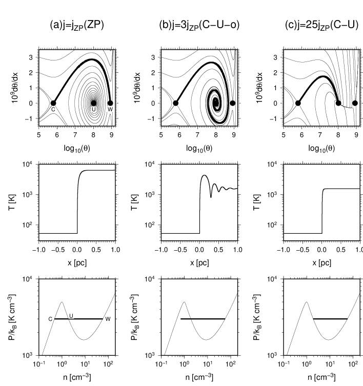
Figure 2: Properties of solutions for $j/j_{\mathrm{ZP}}=1$(a), $3$(b), and $25$(c). The first row indicates the trajectories of solutions with various boundary conditions. The obtained solution satisfying equation (13) are shown by the thick lines. The labels ‘C’, ‘U’, and ‘W’ denote the CNM, unstable phase, and WNM. The second row shows the temperature profile in each mass flux. The third row represents trajectory of the obtained solution in the $(n,P)$ plane.

It is found that solutions for larger mass flux can be divided by four type solutions: C-U-o, C-U, C-c, and C-C. We describe the property of each solution below.

C-U-o Solutions. For the case with $j=3j_{\mathrm{ZP}}$, the solution does not reaches the saddle point of the WNM but approaches the spiral point of the unstable phase (see the first row of figure 2b). From the second row of figure 2(b), one can see the oscillation of the temperature profile that corresponds to the spiral motion in the phase diagram. The third row shows the trajectory of the solution in the $(n,P)$ plane. The solution truncates at the heating-dominated region before arriving at the WNM. The truncation point corresponds to the peak of the temperature in the second row of figure 2(b). Since the mass flux is still low, the pressure is almost constant. This type solutions already has been found in Elphick, Regev & Shaviv (1992) under the isobaric approximation and a more simplified cooling rate. Inoue, Inutsuka & Koyama (2006) also found them as the finite extent solutions, and they truncated the solution at the first peak of the temperature profile near the transition front. We call this type of solutions ‘C-U-o’ solutions, where ‘C-U’ means solutions connecting CNM and unstable phase, and ‘o’ means the oscillation.

C-U Solutions. For larger mass flux $j=25j_{\mathrm{ZP}}$, the topological properties of the stationary point of the unstable phase changes from spiral to node (see the first row of figure 2c) . Thus, from the second row of figure 2(c), there is no oscillation in the temperature profile, and the CNM is monotonically connected with the unstable phase. Figure 3 shows solutions for much larger mass flux, $j/j_{\mathrm{ZP}}=25$, 1000, 2000, and 3000. One can see that as the mass flux increases, the density (pressure) of the unstable phase at $x=\infty$ increases (decreases) along the equilibrium curve. Because of large mass flux, the pressure increases significantly toward the CNM. This type solutions with lower mass flux already has been found in Elphick, Regev & Shaviv (1992) under isobaric approximation. We call this type of solutions ‘C-U’ solutions.

Figure 3: Trajectories of solutions for $j/j_{\mathrm{ZP}}=1$(the solid line), 1000(the dashed line), 2000(the dotted line), 3000(the dot-dashed line). The CNM pressure is set to $P_{\mathrm{c}}=3000k_{\mathrm{B}}$ K cm^-3. The filled circle shows the state at $x=\infty$.

Figure 4: Trajectories of solutions for $j/j_{\mathrm{ZP}}=300$(the solid line), 500(the dashed line), 1000(the dotted line), 1500(the dot-dashed line). The CNM pressure is set to $P_{\mathrm{c}}=4000k_{\mathrm{B}}$ K cm^-3. The filled circle shows the state at $x=\infty$.

C-c Solutions. Figure 4 shows the solutions for $j/j_{\mathrm{ZP}}=300$, 500, 1000, and 1500. Here, we set $P_{\mathrm{c}}/k_{\mathrm{B}}=4000$ K cm^-3. The corresponding mass flux is $j_{\mathrm{ZP}}=-2.15\times 10^{-2}m_{\mathrm{H}}$ km s^-1. The solution for $j=300j_{\mathrm{ZP}}$ belongs to the C-U solution. For larger mass flux $j=500j_{\mathrm{ZP}}$, the solution truncates at a certain point before arriving at the equilibrium state. This critical point corresponds to $T=T_{\mathrm{crit}}=M^{2}/(4{\cal R}j^{2})$ above which solutions do not exist (see equation (9)-(11)). The physical variables at the critical point is denoted by using the subscript of ‘crit’. From equations (6) and (7), the condition $T=T_{\mathrm{crit}}$ is equivalent to

$$|v_{\mathrm{crit}}|=\sqrt{P_{\mathrm{crit}}/\rho_{\mathrm{crit}}}.$$ (17)

Note that equation (17) is slightly smaller than the adiabatic sound speed $\sqrt{\gamma P_{\mathrm{crit}}/\rho_{\mathrm{crit}}}$. These critical velocity and temperature are also seen in the steady state structure of the shock front with heat conduction without physical viscosity (Zel’dovich & Raizer, 1967). At the critical point, one can see that equation (12) becomes infinity. Thus, in order to obtain a finite solution, $d\theta/dx$ must vanish at the critical point. From equations (11) and (12), the pressure gradient becomes finite as follows:

$$\left(\frac{dP}{dx}\right)_{\mathrm{crit}} = -\left(\frac{2{\cal R}j^{2}}{\sqrt{M^{2}-4{\cal R}j^{2}T}}\frac{dT}{dx}\right)_{\mathrm{crit}}$$

$$= -\left(\rho{\cal L}_{\mathrm{crit}}\right)\sqrt{\frac{\rho_{\mathrm{crit}}}{P_{\mathrm{crit}}}}$$

The pressure at the critical point can be derived from the momentum flux conservation. At the CNM $(x=-\infty)$, since the velocity is still subsonic because of its high density, the momentum flux becomes

$$M=\rho_{\mathrm{c}}v_{\mathrm{c}}^{2}+P_{\mathrm{c}}\simeq P_{\mathrm{c}}.$$ (19)

On the other hand, from equation (11), the pressure at the critical point is given by $P_{\mathrm{crit}}=M/2$. Therefore, the pressure at the critical point can be expressed by $P_{\mathrm{c}}$ as follows:

$$P_{\mathrm{crit}}\simeq P_{\mathrm{c}}/2.$$ (20)

The density at the critical point is given by

$$\rho_{\mathrm{crit}}=j^{2}/P_{\mathrm{crit}}\simeq 2j^{2}/P_{\mathrm{c}}.$$ (21)

One can see that $P_{\mathrm{crit}}$ for $j=500j_{\mathrm{ZP}}$ and 1000$j_{\mathrm{ZP}}$ is roughly equal to $P_{\mathrm{c}}/2=2000k_{\mathrm{B}}$ K cm^-3, and its density increases for larger mass flux as seen in equation (21). Around the critical point, since $dT/dx=d\theta/dx/\kappa=0$, the trajectories in the $(n,P)$ plane approach constant temperature lines of $T=T_{\mathrm{crit}}$ in figure 4.

We investigate the topological properties at the critical point in the phase diagram. The Jacobi matrix of equation (12) around the critical point becomes infinite. Thus, there is no solution passing the critical point smoothly. In order to obtain infinite extent solution, shock front is required. Solutions with shock front are described in Appendix A. We call this type of solutions “C-c” solution, where “C-c” means solutions connecting the CNM and the critical point.

C-C Solutions. For much larger mass flux case $j=1500j_{\mathrm{ZP}}$, since the solution passes the equilibrium curve before arriving at the critical point, the solution becomes the infinite extent solution connecting the CNM and CNM (see figure 4). We call this type of solutions C-C solutions, where ‘C-C’ means solutions connecting the CNM and CNM.

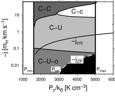
Figure 5: Classification diagram of obtained solutions in parameter space $(P_{\mathrm{c}},j)$. The white dashed line corresponds to $j_{\mathrm{ZP}}$. The solid line indicates the critical mass flux $j_{\mathrm{crit}}(P_{\mathrm{c}})$. The black area where $|j|<|j_{\mathrm{ZP}}|$ is not focused in this paper.

Figure 5 shows classification of solutions in the parameter space $(P_{\mathrm{c}},j)$ for $P_{\mathrm{min}}<P_{\mathrm{c}}<P_{\mathrm{max}}$. The white dashed line corresponds to $j=j_{\mathrm{ZP}}(P_{\mathrm{c}})$ on which the ZP solutions exist. The black area where $|j|<|j_{\mathrm{ZP}}|$ is not focused in this paper. From figure 5, one can see that C-c solutions exist only for $P_{\mathrm{c}}>2P_{\mathrm{min}}$. This is because if $P_{\mathrm{c}}<2P_{\mathrm{min}}$, the solutions meet the equilibrium state before arriving at the critical point (see equation (20)).

4.1.2 Structure of Transition Layers

We investigate how the structure of transition layers depends on the mass flux. As mentioned in section 3, in the ZP solutions, the thickness of the front is characterized by the Field length because the mass flux is very small. As $|j|$ increases, the effect of advection (the first term of equation (8)) becomes important compared with the heat conduction (the third term of equation (8)) in the energy transfer. We can define a critical mass flux $j_{\mathrm{crit}}$ where the effect of advection becomes comparable to the heat conduction as follows:

$$-c_{p}j_{\mathrm{crit}}\frac{T_{\mathrm{m}}}{l_{\mathrm{F,m}}}=\kappa\frac{T_{\mathrm{m}}}{l_{\mathrm{F,m}}^{2}}\Rightarrow j_{\mathrm{crit}}=-\frac{l_{\mathrm{F,m}}}{\gamma l_{\mathrm{c,m}}}\rho_{\mathrm{m}}c_{\mathrm{m}},$$ (22)

where the subscript ‘m’ denotes a reference state in the solutions, $l_{\mathrm{c,m}}$ is the cooling length defined by

$$l_{\mathrm{c,m}}=c_{m}\frac{P_{\mathrm{m}}}{(\gamma-1)\rho_{\mathrm{m}}{\cal L}_{\mathrm{m}}},$$ (23)

and $c_{\mathrm{m}}=\sqrt{\gamma P_{\mathrm{m}}/\rho_{\mathrm{m}}}$ is the sound speed. As the reference state, we consider the state where $|\cal L|$ has the maximum value for $T>T_{\mathrm{c}}$ under the constant pressure $P=P_{\mathrm{c}}$. This state roughly gives minimum Field length and cooling length in the solution. Thus, the critical mass flux is a function of $P_{\mathrm{c}}$. The actual value of $j_{\mathrm{crit}}$ is shown by the solid line in figure 7. In most range of $P_{\mathrm{c}}$, $j_{\mathrm{crit}}$ lies in the region occupied by the C-U solutions.

For $|j|>|j_{\mathrm{crit}}|$, advection dominates heat conduction in energy transfer. In this case, the thickness of the front is characterized by the cooling length instead of the Field length. In typical ISM, $l_{\mathrm{F}}/l_{\mathrm{c}}$ is roughly as small as $10^{-2}$. Therefore, as the mass flux increases, the thickness of the front increases. Figure 6 shows the temperature profiles for $j=j_{\mathrm{ZP}}$, $j_{\mathrm{crit}}$, $5j_{\mathrm{crit}}$, and $10j_{\mathrm{crit}}$. The CNM pressure is set to $P_{\mathrm{c}}/k_{\mathrm{B}}=3000$ K cm^-3. One can see that the thickness of the layer increases with the mass flux.

Figure 6: Temperature profiles for $j=j_{\mathrm{ZP}}$(the solid line), $j_{\mathrm{crit}}$(the dashed line), $5j_{\mathrm{crit}}$(the dotted line), and $10j_{\mathrm{crit}}$(the dot-dashed line). The CNM pressure is set to $P_{\mathrm{c}}/k_{\mathrm{B}}=300$ K cm^-3.

4.2 Transition Layers for $P_{\mathrm{c}}>P_{\mathrm{max}}$

In previous section, we found solutions only for $P_{\mathrm{min}}<P_{\mathrm{c}}<P_{\mathrm{max}}$. However, in actual ISM, the CNM pressure can be greater than $P_{\mathrm{max}}$, for example, in shock-compressed regions. Our solutions can be directly extend for $P_{\mathrm{c}}>P_{\mathrm{max}}$.

Figure 7 is the same as figure 5 but it includes the pressure range of $P_{\mathrm{c}}>P_{\mathrm{max}}$. Figure 7 shows that most of the regions are covered by the C-c solution for $P_{\mathrm{c}}>P_{\mathrm{max}}$. The area of C-U solutions spreads to the pressure range of $P_{\mathrm{max}}<P_{\mathrm{c}}<2P_{\mathrm{max}}$. This is because solutions in this pressure range can connect with thermal equilibrium states before reaching at the critical point at a certain range of $j$. Figure 8 shows trajectories of the solutions for $j/j_{\mathrm{crit}}=1$, 2, 5, and 20. The CNM pressure is set to $2.65\times 10^{4}$ K cm^-3. One can see that the solution terminates at the critical point whose pressure is equal to $P_{\mathrm{c}}/2$ and where density increases with the mass flux.

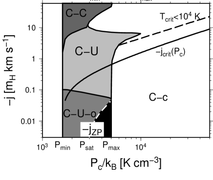
Figure 7: The same as figure 5 but including the pressure range of $P_{\mathrm{c}}>P_{\mathrm{max}}$. The dashed line corresponds to $T_{\mathrm{crit}}=10^{4}$ K.

Figure 8: Trajectories of solutions for $j/j_{\mathrm{crit}}=1$, 2, 5, and 20. The dashed line corresponds to $P=P_{\mathrm{crit}}/2$.

5 Discussion

5.1 Implications

Koyama & Inutsuka (2006) have investigated multi-dimensional nonlinear development of the TI without external forcing. They found that the turbulence is self-sustained by the TI. The velocity dispersion for sufficiently large simulation box is as large as $\sim 0.2-0.4$ km s^-1. They suggested that this velocity is much larger than the prediction in ZP69. Our solutions exist in such a large mass flux. From their simulation, the mass flux becomes $|j|\sim 0.2\;m_{\mathrm{H}}\;\mathrm{km\;s^{-1}}(n/0.5\;\mathrm{cm^{-3}})(v/0.4\;\mathrm{km\;s^{-1}})$, where we assume that the accretion velocity to the CNM is comparable to this velocity dispersion. From figure 5, the corresponding solutions lie in the C-U or C-U-o solutions.

Koyama & Inutsuka (2002) have investigated the TI in the shock-compressed region. They found that the velocity dispersion is as large as several km s^-1. The corresponding mass flux is $|j|\sim 20\;m_{\mathrm{H}}\;\mathrm{km\;s^{-1}}(n/10\;\mathrm{cm^{-3}})(v/2\;\mathrm{km\;s^{-1}})$ that is larger than the results in Koyama & Inutsuka (2006). The pressure of the shock compressed region is larger than $P_{\mathrm{max}}$, indicting that the two stable phases cannot coexist. In shock compressed regions, the CNM clouds are embedded not by the stable WNM but by the unstable gas that is supplied continuously by shock compression. The C-c solutions in this pressure range $(P>P_{\mathrm{max}})$ may describe dynamical condensation from the unstable gas to the CNM in shock compression regions.

5.2 Curvature Effect

Our solutions are derived by assuming the plane-parallel geometry. Nagashima, Koyama & Inutsuka (2005) investigated the curvature effect of the transition front by assuming the quasi-steady approximation. They consider the cylindrical and spherical CNM cloud at the centre. In contrast to the plane parallel solutions, the solutions have three parameters, the pressure of the CNM, the velocity of the front with respect to the centre, and the cloud radius. The second parameter corresponds to the mass flux in our solutions. They solved equations as the eigen- and boundary-value problem so that the solutions connect the CNM and WNM. Thus, the velocity of the front $v_{f}(P_{\mathrm{c}},R_{\mathrm{c}})$ is a function of $P_{\mathrm{c}}$ and cloud radius $R_{\mathrm{c}}$. The curvature effect enhance the heat flux by the thermal conduction from the CNM to the WNM. Thus, smaller cloud that has larger curvature tends to evaporate quickly. On the other hand, cold gas that has a negative curvature tends to gain mass by the condensation. Thus, the evolution of CNM cloud strongly depends on its shape.

By using the quasi-steady approximation, we can easily take into account curvature effect in our solutions. It is expected that solutions with larger evaporation rate connect the unstable phase and WNM while solutions with larger condensation rate connect the CNM and unstable phase.

6 Summary

In this paper, we have investigated steady condensation solutions of phase transition layers in large parameter space $(P_{\mathrm{c}},j)$ much larger than previous works. We summarise our results as follows:

• In the pressure range where the three thermal equilibrium phase can coexist under a constant pressure $(P_{\mathrm{min}}<P_{\mathrm{c}}<P_{\mathrm{max}})$, we find solutions that connects the CNM and the unstable phase. The solutions can be classified into four type solutions, C-U-o, C-U, C-c, and C-C solutions in order of the mass flux. The C-U-o and C-U solutions connect the CNM and the unstable phase with and without the oscillation of physical quantities in the low-density side. The C-c solution is truncated at the maximum temperature above which there are no steady solutions. Combination of a C-c solution and a shock front provides an infinite extent solution. The C-C solutions connect the CNM and CNM.

• We have also found steady solutions in the pressure range $(P_{\mathrm{c}}>P_{\mathrm{max}})$ where only CNM can be in equilibrium. This pressure range is realized in the shock compressed region. In this parameter space $(P_{\mathrm{c}},j)$, most of solutions belong to the C-c solution.

• We derived a critical mass flux $j_{\mathrm{crit}}$ above which the effect of advection becomes important compared with the heat conduction in energy transfer. For large mass flux, $|j|>|j_{\mathrm{crit}}|$, the thickness of the front is characterized by the cooling length instead of the Field length, so that the thickness becomes larger.

Appendix A Solutions with Shock Front

In this Appendix, we present steady solutions with shock front. Here, we assume that preshock gas is in thermal equilibrium state. The physical variables in preshock gas are denoted by using the subscript of “E”. The position of the shock front $x=x_{\mathrm{sh}}$ is determined so that the Rankine-Hugoniot relation is satisfied between the solutions and the thermal equilibrium state by the following method. Given $x=x_{\mathrm{sh}}$, the specific energy flux is given by

$$\frac{\gamma P_{\mathrm{sh}}}{(\gamma-1)\rho_{\mathrm{sh}}}+\frac{1}{2}v_{\mathrm{sh}}^{2}\equiv\frac{\gamma+1}{2(\gamma-1)}c_{*}^{2},$$ (24)

where the subscript of “sh” denotes physical variables at $x=x_{\mathrm{sh}}$, and $c_{*}^{2}$ is the effective sound speed. The simple relation among $v_{\mathrm{sh}}$, $v_{\mathrm{E}}$, and $c_{*}$ is given by

$$v_{\mathrm{sh}}v_{\mathrm{E}}=c_{*}^{2}.$$ (25)

From equation (25), one can get $v_{\mathrm{E}}$, and the Mach number ${\cal M}$ is obtained. From the Rankine-Hugoniot relations, the physical variables in the preshock gas ($\rho_{\mathrm{E}}$ and $T_{\mathrm{E}}$) are obtained. In general, the preshock gas is not in thermal equilibrium state. The position of the shock front $x_{\mathrm{sh}}$ is determined iteratively until ${\cal L}(\rho_{\mathrm{E}},T_{\mathrm{E}})=0$ is satisfied by using the bisection method.

As examples, we consider two cases of $j=2$ and 24$j_{\mathrm{crit}}$ for $P_{\mathrm{c}}/k_{\mathrm{B}}=3.114\times 10^{4}$K cm^-3. For $j=2j_{\mathrm{c}}$ case, the corresponding physical quantities of the preshock gas are $n_{\mathrm{E}}=0.57$ cm^-3 and ${\cal M}=2.17$. For $j=24j_{\mathrm{c}}$, they are $n_{\mathrm{E}}=75$ cm^-3 and ${\cal M}=2.23$. Thus, the preshock gases belong to the WNM for $j=2j_{\mathrm{c}}$ and CNM for $j=24j_{\mathrm{crit}}$. The upper panels of figures 9a and 9b show the density, temperature, and pressure distribution for $j=2j_{\mathrm{crit}}$ and $j=24j_{\mathrm{crit}}$, respectively. The lower panels of figure 9 show the trajectories of obtained solutions in the $(n,P)$ plane.

In addition, we perform one-dimensional hydrodynamical simulation in order to confirm the steady state solutions with shock front are realized. We consider colliding wall problem where the gas flows collide at $x=0$ with $|v_{\mathrm{E}}-v_{\mathrm{c}}|$ from $x=\pm\infty$. Two shock wave propagates from $x=0$ outward. Shock heated gas quickly cools until the gas reaches the thermal equilibrium state. After that, the cold layer forms and its thickness grows by gas accretion. The thick gray line in each panel of figure 9 indicate the results of one-dimensional simulations in the growing phase of the cold layer. One can see that the results of one-dimensional simulations are well described by the steady-state solutions.

Figure 9: Upper panels: Density (solid line), temperature (dashed line), and pressure (dotted line) profiles of steady state solutions at which $P_{\mathrm{c}}=3.113\times 10^{4}$ K cm^-3 for (a)$j=2j_{\mathrm{crit}}$ and (b)$j=24j_{\mathrm{crit}}$. Lower panels: Trajectories of steady state solutions in the $(n,P)$ plane. The thick gray line in each panel shows the results of one-dimensional hydrodynamical simulation.

References

- Audit & Hennebelle (2005) Audit, E., & Hennebelle, P. 2005, A&A, 433, 1
- Audit & Hennebelle (2010) Audit, E., & Hennebelle, P. 2010, A&A, 511, 76
- Balbus (1986) Balbus, S. A. 1986, ApJ, 303, 79
- Belgelman & McKee (1990) Begelman, M. C., & McKee, C. F. 1990, ApJ, 358, 375
- Elphick, Regev & Shaviv (1992) Elphick, C., Regev, O., & Shaviv, N. 1992, ApJ, 392, 106
- Ferrara & Shchekinov (1993) Ferrara, A., & Shchekinov, Yu. A. 1993, ApJ, 417, 595
- Field (1965) Field, G. B. 1965, ApJ, 142, 531
- Field, Goldsmith & Habing (1969) Field, G. B., Goldsmith, D. W., & Habing, H. J. 1969, ApJ, 155, L149
- Gazol, Vázquez-Semadeni & Kim (2005) Gazol, A., Vázquez-Semadeni, E., & Kim, J. 2005, ApJ, 630, 911
- Graham & Langer (1973) Graham, R., & Langer, W. D. 1973, ApJ, 179, 469
- Heitsch et al. (2005) Heitsch, F., Burkert, A., Hartmann, L., Slyz, A., & Devriendt, J. 2005, ApJ, 633, 113
- Heitsch et al. (2006) Heitsch, F., Slyz, A., Devriendt, J., Hartmann, L., & Burkert, A. 2006, ApJ, 647, 1052
- Heitsch, Stone & Hartmann (2009) Heitsch, F., Stone, J., & Hartmann, L. 2009, ApJ, 695, 248
- Hennebelle & Audit (2007) Hennebelle, P., & Audit, E. 2007, A&A, 465, 431
- Hennebelle et al. (2008) Hennebelle, P., Banerjee, R., Vázquez-Semadeni, E., Klessen, R., & Audit, E. 2008, A&A, 486, L43
- Inoue & Inutsuka (2008) Inoue, T., & Inutsuka, S., 2008, ApJ, 687, 303
- Inoue & Inutsuka (2009) Inoue, T., & Inutsuka, S., 2009, ApJ, 704, 161
- Inoue, Inutsuka & Koyama (2006) Inoue, T., Inutsuka, S., & Koyama, H. 2006, ApJ, 652, 1331
- Iwasaki & Tsuribe (2008) Iwasaki, K., & Tsuribe, T. 2008, MNRAS, 387, 1554
- Iwasaki & Tsuribe (2009) Iwasaki, K., & Tsuribe, T. 2009, A&A, 508, 725
- Kritsuk & Norman (2002) Kritsuk, A. G., & Norman, M. L. 2002, ApJ, 569, L127
- Koyama & Inutsuka (2002) Koyama, H, & Inutsuka, S. 2002, ApJ, 564, L97
- Koyama & Inutsuka (2006) Koyama, H, & Inutsuka, S. 2006, [arXiv:astro-ph/0605528]
- Landau & Lifshitz (1987) Landau, L. D., & Lifshitz, E. 1987, Fluid Mechanics. Pergamon, New York
- Nagashima, Koyama & Inutsuka (2005) Nagashima, M., Koyama, H., & Inutsuka, S., 2005, MNRAS, 361, L25
- Parker (1953) Parker, E. N. 1953, ApJ, 117, 431
- Penston & Brown (1970) Penston, M. V., & Brown, F. E. 1970, MNRAS, 150, 373