Time and Space Efficient Lempel-Ziv Factorization based on Run Length Encoding

Abstract

We propose a new approach for calculating the Lempel-Ziv factorization of a string, based on run length encoding (RLE). We present a conceptually simple off-line algorithm based on a variant of suffix arrays, as well as an on-line algorithm based on a variant of directed acyclic word graphs (DAWGs). Both algorithms run in $O(N+n\log n)$ time and $O(n)$ extra space, where $N$ is the size of the string, $n\leq N$ is the number of RLE factors. The time dependency on $N$ is only in the conversion of the string to RLE, which can be computed very efficiently in $O(N)$ time and $O(1)$ extra space (excluding the output). When the string is compressible via RLE, i.e., $n=o(N)$, our algorithms are, to the best of our knowledge, the first algorithms which require only $o(N)$ extra space while running in $o(N\log N)$ time.

1 Introduction

The run-length encoding (RLE) of a string $S$ is a natural encoding of $S$, where each maximal run of character $a$ of length $p$ in $S$ is encoded as $a^{p}$, e.g., the RLE of string $\mathtt{aaaabbbaa}$ is $\mathtt{a^{4}b^{3}a^{2}}$. Since RLE can be regarded as a compressed representation of strings, it is possible to reduce the processing time and working space if RLE strings are not decompressed while being processed. Many efficient algorithms that deal with RLE versions of classical problems on strings have been proposed in the literature (e.g.: exact pattern matching [7, 4, 2], approximate matching [26, 3], edit distance [8, 5, 24, 10], longest common subsequence [17, 25], rank/select structures [22], palindrome detection [11]). In this paper, we consider the problem of computing the Lempel-Ziv factorization (LZ factorization) of a string via RLE.

The LZ factorization (and its variants) of a string [35, 32, 13], discovered over 30 years ago, captures important properties concerning repeated occurrences of substrings in the string, and has applications in the field of data compression, as well as being the key component to various efficient algorithms on strings [20, 16]. Therefore, there exists a large amount of work devoted to its efficient computation. A naïve algorithm that computes the longest common prefix with each of the $O(N)$ previous positions only requires $O(1)$ space (excluding the output), but can take $O(N^{2})$ time, where $N$ is the length of the string. Using string indicies such as suffix trees [34] and on-line algorithms to construct them [33], the LZ factorization can be computed in an on-line manner in $O(N\log|\Sigma|)$ time and $O(N)$ space, where $|\Sigma|$ is the size of the alphabet. Most recent algorithms [9, 15, 14, 1, 29] first construct the suffix array [27] of the string, consequently taking $O(N)$ extra space and at least $O(N)$ time, and are off-line.

Since the most efficient algorithms run in worst-case linear time and are practical, it may seem that not much better can be achieved. However, a theoretical interest is whether or not we can achieve even faster algorithms, at least in some specific cases. In this paper, we propose a new approach for calculating the Lempel-Ziv factorization of a string, which is based on its RLE. The contributions of this paper are as follows: We first show that the size of the LZ encoding with self-references (i.e., allowing previous occurrences of a factor to overlap with itself) is at most twice as large as the size of its RLE. We then present two algorithms that compute the LZ factorizations of strings given in RLE: an off-line algorithm based on suffix arrays for RLE strings, and an on-line algorithm based on directed acyclic word graphs (DAWGs) [6] for RLE strings. Given an RLE string of size $n$, both algorithms work for general ordered alphabets, and run in $O(n\log n)$ time and $O(n)$ space. Since the conversion from a string of size $N$ to its RLE can be conducted very efficiently in $O(N)$ time and $O(1)$ extra space (excluding the output), the total complexity is $O(N+n\log n)$ time and $O(n)$ space.

In the worst-case, the string is not compressible by RLE, i.e. $n=N$. Thus, for integer alphabets, our approach can be slightly slower than the fastest existing algorithms which run in $O(N)$ time (off-line) or $O(N\log|\Sigma|)$ time (on-line). However, for general ordered alphabets, the worst-case complexities of our algorithms match previous algorithms since the construction of the suffix array/suffix tree can take $O(N\log N)$ time if $|\Sigma|=O(N)$. The significance of our approach is that it allows for improvements in the computational complexity of calculating the LZ factorization for a non-trivial family of strings; strings that are compressible via RLE. If $n=o(N)$, our algorithms are, to the best of our knowledge, the first algorithms which require only $o(N)$ extra space while running in $o(N\log N)$ time.

Related Work. For computing the LZ78 [36] factorization, a sub-linear time and space algorithm was presented in [18]. In this paper, we consider a variant of the more powerful LZ77 [35] factorization. Two space efficient on-line algorithms for LZ factorization based on succinct data structures have been proposed [30, 31]. The first runs in $O(N\log^{3}N)$ time and $N\log|\Sigma|+o(N\log|\Sigma|)+O(N)$ bits of space [30], and the other runs in $O(N\log^{2}N)$ time with $O(N\log|\Sigma|)$ bits of space [31]. Succinct data structures basically simulate accesses to their non-succinct counterparts using less space at the expense of speed. A notable distinction of our approach is that we aim to reduce the problem size via compression, in order to improve both time and space efficiency.

2 Preliminaries

Let $\mathcal{N}$ be the set of non-negative integers. Let $\Sigma$ be a finite alphabet. An element of $\Sigma^{*}$ is called a string. The length of a string $S$ is denoted by $|S|$. The empty string $\varepsilon$ is the string of length 0, namely, $|\varepsilon|=0$. For any string $S\in\Sigma$, let $\sigma_{S}$ denote the number of distinct characters appearing in $S$. Let $\Sigma^{+}=\Sigma^{*}-\{\varepsilon\}$. For a string $S=XYZ$, $X$, $Y$ and $Z$ are called a prefix, substring, and suffix of $S$, respectively. The set of prefixes of $S$ is denoted by $\mathit{Prefix}(S)$. The longest common prefix of strings $X,Y$, denoted $\mathit{lcp}(X,Y)$, is the longest string in $\mathit{Prefix}(X)\cap\mathit{Prefix}(Y)$. The $i$-th character of a string $S$ is denoted by $S[i]$ for $1\leq i\leq|S|$, and the substring of a string $S$ that begins at position $i$ and ends at position $j$ is denoted by $S[i..j]$ for $1\leq i\leq j\leq|S|$. For convenience, let $S[i..j]=\varepsilon$ if $j<i$.

For any character $a\in\Sigma$ and $p\in\mathcal{N}$, let $a^{p}$ denote the concatenation of $p$ $a$’s, e.g., $a^{1}=a$, $a^{2}=aa$, and so on. $p$ is said to be the exponent of $a^{p}$. Let $a^{0}=\varepsilon$.

Our model of computation is the word RAM with the computer word size at least $\lceil\log_{2}|S|\rceil$ bits, and hence, standard instructions on values representing lengths and positions of string $S$ can be executed in constant time. Space complexities will be determined by the number of computer words (not bits).

2.1 LZ Encodings

LZ encodings are dynamic dictionary based encodings with many variants. As in most recent work, we describe our algorithms with respect to a well known variant called s-factorization [13] in order to simplify the presentation.

Definition 1 (s-factorization [13])

The s-factorization of a string $S$ is the factorization $S=f_{1}\cdots f_{n}$ where each s-factor $f_{i}\in\Sigma^{+}~{}(i=1,\ldots,n)$ is defined inductively as follows: $f_{1}=S[1]$. For $i\geq 2$: if $S[|f_{1}\cdots f_{i-1}|+1]=c\in\Sigma$ does not occur in $f_{1}\cdots f_{i-1}$, then $f_{i}=c$. Otherwise, $f_{i}$ is the longest prefix of $f_{i}\cdots f_{n}$ that occurs at least twice in $f_{1}\cdots f_{i}$.

Note that each s-factor can be represented in constant size, i.e., either as a single character or a pair of integers representing the position of a previous occurrence of the factor and its length. For example the s-factorization of the string $S=\mathtt{abaabababaaaaabbabab}$ is $\mathtt{a}$, $\mathtt{b}$, $\mathtt{a}$, $\mathtt{aba}$, $\mathtt{baba}$, $\mathtt{aaaa}$, $\mathtt{b}$, $\mathtt{babab}$. This can be represented as $\mathtt{a}$, $\mathtt{b}$, $(1,1)$, $(1,3)$, $(5,4)$, $(10,4)$, $(2,1)$, $(5,5)$. In this paper, we will focus on describing algorithms that output only the length of each factor of the s-factorization, but it is not difficult to modify them to output the previous position as well, in the same time and space complexities.

2.2 Run Length Encoding

Definition 2

The Run-Length (RL) factorization of a string $S$ is the factorization $f_{1},\ldots,f_{n}$ of $S$ such that for every $i=1,\ldots,n$, factor $f_{i}$ is the longest prefix of $f_{i}\cdots f_{n}$ with $f_{i}\in\{a^{p}\mid a\in\Sigma,p>0\}$.

Note that each factor $f_{i}$ can be written as $f_{i}=a_{i}^{p_{i}}$ for some character $a_{i}\in\Sigma$ and some integer $p_{i}>0$ and for any consecutive factors $f_{i}=a_{i}^{p_{i}}$ and $f_{i+1}=a_{i+1}^{p_{i+1}}$, we have that $a_{i}\neq a_{i+1}$. The run length encoding (RLE) of a string $S$, denoted $\mathit{RLE}_{S}$, is a sequence of pairs consisting of a character $a_{i}$ and an integer $p_{i}$, representing the RL factorization. The size of $\mathit{RLE}_{S}$ is the number of RL factors in $\mathit{RLE}_{S}$ and is denoted by $\mathit{size}(\mathit{RLE}_{S})$, i.e., if $\mathit{RLE}_{S}=a_{1}^{p_{1}}\cdots a_{n}^{p_{n}}$, then $\mathit{size}(\mathit{RLE}_{S})=n$. $\mathit{RLE}_{S}$ can be computed in $O(N)$ time and $O(1)$ extra space (excluding the $O(n)$ space for output), where $N=|S|$, simply by scanning $S$ from beginning to end, counting the exponent of each RL factor. Also, noticing that each RL factor must consist of the same alphabet, we have $\sigma_{S}\leq n$.

Let $\mathit{val}$ be the function that “decompresses” $\mathit{RLE}_{S}$, i.e., $\mathit{val}(\mathit{RLE}_{S})=S$. For any $1\leq i\leq j\leq n$, let $\mathit{RLE}_{S}[i..j]=a^{p_{i}}_{i}a^{p_{i+1}}_{i+1}\cdots a^{p_{j}}_{j}$. For convenience, let $\mathit{RLE}_{S}[i..j]=\varepsilon$ if $i>j$. Let $\mathit{RLE\_Substr}(S)=\{\mathit{RLE}_{S}[i..j]\mid 1\leq i,j\leq n\}$ and $\mathit{RLE\_Suffix}(S)=\{\mathit{RLE}_{S}[i..n]\mid 1\leq i\leq n\}$.

The following simple but nice observation allows us to represent the complexity of our algorithms in terms of $\mathit{size}(\mathit{RLE}_{S})$.

Lemma 1

For a given string $S$, let $n_{\mathit{RL}}$ and $n_{\mathit{LZ}}$ respectively be the number of factors in its RL factorization and s-factorization. Then, $n_{\mathit{LZ}}\leq 2n_{\mathit{RL}}$.

Proof

Consider an s-factor that starts at the $j$th position in some RL-factor $a_{i}^{p_{i}}$ where $1<j\leq p_{i}$. Since $a_{i}^{p_{i}-j+1}$ is both a suffix and a prefix of $a_{i}^{p_{i}}$, we have that the s-factor extends at least to the end of $a_{i}^{p_{i}}$. This implies that a single RL-factor is always covered by at most 2 s-factors, thus proving the lemma.

Note that for LZ factorization variants without self-references, the size of the output LZ encoding may come into play, when it is larger than $O(\mathit{size}(\mathit{RLE}_{S}))$.

2.3 Priority Search Trees

In our LZ factorization algorithms, we will make use the following data structure, which is essentially an elegant mixture of a priority heap and balanced search tree.

Theorem 2.1 (McCreight [28])

For a dynamic set $D$ which contains $n$ ordered pairs of integers, the priority search tree (PST) data structure supports all the following operations and queries in $O(\log n)$ time, using $O(n)$ space:

• $\mathit{Insert}(x,y)$: Insert a pair $(x,y)$ into $D$;

• $\mathit{Delete}(x,y)$: Delete a pair $(x,y)$ from $D$;

• $\mathit{MinXInRectangle}(L,R,B)$: Given three integers $L\leq R$ and $B$, return the pair $(x,y)\in D$ with minimum $x$ satisfying $L\leq x\leq R$ and $y\geq B$;

• $\mathit{MaxXInRectangle}(L,R,B)$: Given three integers $L\leq R$ and $B$, return the pair $(x,y)\in D$ with maximum $x$ satisfying $L\leq x\leq R$ and $y\geq B$;

• $\mathit{MaxYInRange}(L,R)$: Given two integers $L\leq R$, return the pair $(x,y)\in D$ with maximum $y$ satisfying $L\leq x\leq R$.

3 Off-line LZ Factorization based on RLE

In this section we present our off-line algorithm for s-factorization. The term off-line here implies that the input string $S$ of length $N$ is first converted to a sequence of RL factors, $\mathit{RLE}_{S}=a_{1}^{p_{1}}a_{2}^{p_{2}}\cdots a_{n}^{p_{n}}$. In the algorithm which follows, we introduce and utilize RLE versions of classic string data structures.

3.1 RLE Suffix Arrays

Let $\Sigma_{\mathit{RLE}_{S}}=\{\mathit{RLE}_{S}[i]\mid i=1,\ldots,n\}$. For instance, if $\mathit{RLE}_{S}=\mathtt{a^{3}b^{5}a^{3}b^{5}a^{1}b^{5}a^{4}}$, then $\Sigma_{\mathit{RLE}_{S}}=\{\mathtt{a^{1}},\mathtt{a^{3}},\mathtt{a^{4}},\mathtt{b^{5}}\}$. For any $a_{i}^{p_{i}},a_{j}^{p_{j}}\in\Sigma_{\mathit{RLE}_{S}}$, let the order $\prec$ on $\Sigma_{\mathit{RLE}_{S}}$ be defined as $a_{i}^{p_{i}}\prec a_{j}^{p_{j}}\iff a_{i}<a_{j},\mbox{ or }a_{i}=a_{j}\mbox{ and }p_{i}<p_{j}.$ The lexicographic ordering on $\mathit{RLE\_Suffix}(S)$ is defined over the order on $\Sigma_{\mathit{RLE}_{S}}$, and our RLE version of suffix arrays [27] is defined based on this order:

Definition 3 (RLE suffix arrays)

For any string $S$, its run length encoded suffix array, denoted $\mathit{RLE\_SA}_{S}$, is an array of length $n=\mathit{size}(\mathit{RLE}_{S})$ such that for any $1\leq i\leq n$, $\mathit{RLE\_SA}_{S}[i]=j$ when $\mathit{RLE}_{S}[j..n]$ is the lexicographically $i$-th element of $\mathit{RLE\_Suffix}(S)$.

Let $\mathit{SparseSuffix}(S)=\{\mathit{val}(s)\mid s\in\mathit{RLE\_Suffix}(S)\}$, namely, $\mathit{SparseSuffix}(S)$ is the set of “uncompressed” RLE suffixes of string $S$. Note that the lexicographic order of $\mathit{RLE\_Suffix}(S)$ represented by $\mathit{RLE\_SA}_{S}$ is not necessarily equivalent to the lexicographic order of $\mathit{SparseSuffix}(S)$. In the running example, $\mathit{RLE\_SA}_{S}=[5,3,1,7,4,2,6]$. However, the lexicographical order for the elements in $\mathit{SparseSuffix}(S)$ is actually $(7,1,3,5,6,2,4)$.

Lemma 2

Given $\mathit{RLE}_{S}$ for any string $S\in\Sigma^{*}$, $\mathit{RLE\_SA}_{S}$ can be constructed in $O(n\log n)$ time, where $n=\mathit{size}(\mathit{RLE}_{S})$.

Proof

Any two RL factors can be compared in $O(1)$ time, so the lemma follows from algorithms such as in [21].

Let $\mathit{RLE\_RANK}_{S}$ be an array of length $n=\mathit{size}(\mathit{RLE}_{S})$ such that $\mathit{RLE\_RANK}_{S}[j]=i\iff\mathit{RLE\_SA}_{S}[i]=j.$ Clearly $\mathit{RLE\_RANK}_{S}$ can be computed in $O(n)$ time provided that $\mathit{RLE\_SA}_{S}$ is already computed. To make the notations simpler, in what follows we will denote $rs(h)=\mathit{RLE\_SA}_{S}[h]$ and $rr(h)=\mathit{RLE\_RANK}_{S}[h]$ for any $1\leq h\leq n$.

For any RLE strings $\mathit{RLE}_{X}$ and $\mathit{RLE}_{Y}$ with $\mathit{val}(\mathit{RLE}_{X})=X$ and $\mathit{val}(\mathit{RLE}_{Y})=Y$, let $\mathit{lcp}(\mathit{RLE}_{X},$ $\mathit{RLE}_{Y})=\mathit{lcp}(X,Y)$, i.e., $\mathit{lcp}(\mathit{RLE}_{X},\mathit{RLE}_{Y})$ is the longest prefix of the “uncompressed” strings $X$ and $Y$. It is easy to see that $Z=\mathit{lcp}(\mathit{RLE}_{X},\mathit{RLE}_{Y})$ can be computed in $O(\mathit{size}(\mathit{RLE}_{Z}))$ time by a naive comparison from the beginning of $\mathit{RLE}_{X}$ and $\mathit{RLE}_{Y}$, adding up the exponent $p_{i}$ of the RL factors while $a_{i}^{p_{i}}=\mathit{RLE}_{X}[i]=\mathit{RLE}_{Y}[i]$, and possibly the smaller exponent of the first mismatching RL factors, provided that they are exponents of the same character.

The following two lemmas imply an interesting and useful property of our data structure; although $\mathit{RLE\_SA}_{S}$ does not necessarily correspond to the lexicographical order of the uncompressed RLE suffixes, RLE suffixes that are closer to a given entry in the $\mathit{RLE\_SA}_{S}$ have longer longest common prefixes with that entry.

Lemma 3

Let $i,j$ be any integers such that $1\leq i<j\leq n$. (1) For any $j^{\prime}>j$, $|\mathit{lcp}(\mathit{RLE}_{S}[rs(i)..n],$ $\mathit{RLE}_{S}[rs(j)..n])|\geq|\mathit{lcp}(\mathit{RLE}_{S}[rs(i)..n],\mathit{RLE}_{S}[rs(j^{\prime})..n])|$. (2) For any $i^{\prime}<i$, $|\mathit{lcp}(\mathit{RLE}_{S}[rs(i)..n],$ $\mathit{RLE}_{S}[rs(j)..n])|\geq|\mathit{lcp}(\mathit{RLE}_{S}[rs(i^{\prime})..n],\mathit{RLE}_{S}[rs(j)..n])|$.

Proof

We only show (1). (2) can be shown by similar arguments. Let

$$k = \min\{t\mid\mathit{RLE}_{S}[rs(i)..rs(i)+t-1]\neq\mathit{RLE}_{S}[rs(j)..rs(j)+t-1]\}\mbox{ and }$$

$$k^{\prime} = \min\{t^{\prime}\mid\mathit{RLE}_{S}[rs(i)..rs(i)+t^{\prime}-1]\neq\mathit{RLE}_{S}[rs(j^{\prime})..rs(j^{\prime})+t^{\prime}-1]\}.$$

Namely, the first $(k-1)$ RL factors of $\mathit{RLE}_{S}[rs(i)..n]$ and $\mathit{RLE}_{S}[rs(j)..n]$ coincide and the $k$th RL factors differ. The same goes for $k^{\prime}$, $\mathit{RLE}_{S}[rs(i)..n]$, and $\mathit{RLE}_{S}[rs(j^{\prime})..n]$. Since $j^{\prime}>j$, $k\geq k^{\prime}$. If $k>k^{\prime}$, then clearly the lemma holds. If $k=k^{\prime}$, then $\mathit{RLE}_{S}[rs(i)+k]\prec\mathit{RLE}_{S}[rs(j)+k]\preceq\mathit{RLE}_{S}[rs(j^{\prime})+k]$. This implies that $|\mathit{lcp}(\mathit{RLE}_{S}[rs(i)+k],\mathit{RLE}_{S}[rs(j)+k])|\geq|\mathit{lcp}(\mathit{RLE}_{S}[rs(i)+k],\mathit{RLE}_{S}[rs(j^{\prime})+k])|$. The lemma holds since for these pairs of suffixes, the RL factors after the $k$th do not contribute to their $\mathit{lcp}$s.

3.2 LZ factorization using $\mathit{RLE\_SA}$

In what follows we describe our algorithm that computes the s-factorization using $\mathit{RLE\_SA}_{S}$. Assume that we have already computed the first $(j-1)$ s-factors $f_{1},f_{2},\ldots,f_{j-1}$ of string $S$. Let $\sum_{h=1}^{j-1}|f_{h}|=\ell-1$, i.e., the next s-factor $f_{j}$ begins at position $\ell$ of $S$. Let $d=\min\{k\mid\sum_{i=1}^{k}(p_{i})\geq\ell\}+1$, i.e., the $(d-1)$-th RL factor $a_{d-1}^{p_{d-1}}$ contains the occurrence of the $\ell$-th character $S[\ell]=a_{d-1}$ of $S$. Let $q=\sum_{i=1}^{d-1}(p_{i})-\ell+1$, i.e., $\mathit{RLE}_{S[\ell..N]}=a_{d-1}^{q}a_{d}^{p_{d}}\cdots a_{n}^{p_{n}}$. Note that $1\leq q\leq p_{d-1}$.

The task next, is to find the longest previously occurring prefix of $a_{d-1}^{q}a_{d}^{p_{d}}\cdots a_{n}^{p_{n}}$ which will be $f_{j}$. The difficulty here, compared to the non-RLE case, is that $f_{j}$ will not necessarily begin at positions in $S$ corresponding to an entry in the $\mathit{RLE\_SA}_{S}$. A key idea of our algorithm is that rather than looking directly for $a_{d-1}^{q}a_{d}^{p_{d}}$ $\cdots$ $a_{n}^{p_{n}}$, we look for the longest previously occurring prefix of $\mathit{RLE}_{S}[d..n]=a_{d}^{p_{d}}\cdots a_{n}^{p_{n}}$ whose occurrence is immediately preceded by $a_{d-1}^{q}$, which will have corresponding entries in $\mathit{RLE\_SA}_{S}$. To compute $f_{j}$ in this way, we use the following lemma:

Lemma 4

Assume the situation mentioned above. Let $k=\max(\{p_{i}\mid a_{i}=a_{d-1},1\leq i\leq d-2\}\cup\{0\})$. (Case 1) If $q=p_{d-1}$ and $q>k$, then $|f_{j}|=\max\{k,1\}$. (Case 2) Otherwise,

$$|f_{j}|=q+\max\{|\mathit{lcp}(\mathit{RLE}_{S}[rs(x_{1})..n],\mathit{RLE}_{S}[d..n])|,|\mathit{lcp}(\mathit{RLE}_{S}[d..n],\mathit{RLE}_{S}[rs(x_{2})..n])|\}$$

where

$$x_{1} = \max\{u\mid 1<rs(u)<d,~{}u<rr(d),~{}a_{rs(u)-1}=a_{d-1},~{}p_{rs(u)-1}\geq q\}\mbox{ and}$$

$$x_{2} = \min\{v\mid 1<rs(v)<d,~{}rr(d)<v,~{}a_{rs(v)-1}=a_{d-1},~{}p_{rs(v)-1}\geq q\}.$$

Proof

Case (1) is when the new s-factor begins at the beginning of the RL-factor $a_{d-1}^{p_{d-1}}$, and must end somewhere inside it. Otherwise (Case (2)), $|f_{j}|$ is at least $q$ since either $q<p_{d-1}$ and $a_{d-1}^{q}=S[\ell..\ell+q-1]=S[\ell-1..\ell+q-2]$ is a prefix of $f_{j}$ due to the self-referencing nature of s-factorization, or, there exists an RL factor $a_{i}^{p_{i}}$ such that $1\leq i\leq d-2$, $a_{d-1}=a_{i}$ and $q\leq p_{i}$. Let $f_{j}=a_{d-1}^{q}X$. Then $X$ is the longest of the longest common prefixes between $\mathit{RLE}_{S}[d..n]$ and $\mathit{RLE}_{S}[h..n]$ for all $1\leq h<d$, that are immediately preceded by $a_{d-1}^{q}$, i.e. $a_{h-1}=a_{d-1}$ and $p_{h-1}\geq q$. It follows from Lemma 3 that of all these $h$, the one with the longest lcp with $\mathit{RLE}_{S}[d..n]$ is either of the entries that are closest to position $rr(d)$ in the suffix array. The positions $x_{1}$ and $x_{2}$ of these entries can be described by the equation in the lemma statement, and thus the lemma holds.

Once $x_{1}$ and $x_{2}$ of the above Lemma are determined, our algorithm is similar to conventional non-RLE algorithms that use the suffix array. The main difficulty lies in computing these values, since, unlike the non-RLE algorithms, they depend on the value $q$ which is determined only during the s-factorization. The main result of this section follows.

Theorem 3.1

Given $\mathit{RLE}_{S}$ of any string $S\in\Sigma^{*}$, we can compute the s-factorization of $S$ in $O(n\log n)$ time and $O(n)$ space where $n=\mathit{size}(\mathit{RLE}_{S})$.

Proof

First, compute $\mathit{RLE\_SA}_{S}$ in $O(n\log n)$ time, and $\mathit{RLE\_RANK}_{S}$ in $O(n)$ time. Next we show how to compute each s-factor $f_{j}$ using Lemma 4.

Recall that the s-factor begins somewhere in the $(d-1)$-th RL factor. We shall maintain, for each character $a\in\Sigma$, a PST $T_{a}$ of Theorem 2.1 for the set of pairs $U_{a}^{d-1}=\{(x,y)\mid x=rr(i),~{}a_{i-1}=a,~{}y=p_{i-1},~{}1<i\leq d-1\}$, i.e., the $x$ coordinate is the position in the suffix array, and the $y$ coordinate is the exponent of the preceding character of that suffix. Then, we can easily check whether the condition of case (1) is satisfied by computing the $k$ of Lemma 4 as $k=\mathit{MaxYInRange}(1,n)$ on $T_{a_{d-1}}$, which can be computed in $O(\log n)$ time by Theorem 2.1. For case (2), we obtain $x_{1}$ and $x_{2}$ as: $x_{1}=\mathit{MaxXInRectangle}(1,rr(d)-1,q)$ and $x_{2}=\mathit{MinXInRectangle}(rr(d)+1,n,q)$ in $O(\log n)$ time, using $T_{a_{d-1}}$. To compute the length of the lcp’s, $\mathit{lcp}(\mathit{RLE}_{S}[rs(x_{1})..n],$ $\mathit{RLE}_{S}[d..n])$ and $\mathit{lcp}(\mathit{RLE}_{S}[d..n],$ $\mathit{RLE}_{S}[rs(x_{2})..n])$, we simply use the naive algorithm mentioned previously, that compares each RL factor from the beginning. Since the longer of the two longest common prefixes is adopted, the number of comparisons is at most twice the number of RL factors that is spanned by the determined s-factor. From Lemma 1, the total number of RL factors compared, i.e. $\sum_{i=1}^{n_{LZ}}\mathit{size}(\mathit{RLE}_{f_{i}})$, is $O(n)$.

After computing the s-factor $f_{j}$, we update the PSTs. Namely, if $f_{j}$ spans the RL factors $a_{d}^{p_{d}}\cdots a_{d+g}^{p_{d+g}}$, then we insert pair $(rr(i),p_{i-1})$ into $T_{a_{i-1}}$, for all $d\leq i\leq d+g$. These insertion operations take $O(g\log n)$ time by Theorem 2.1, which takes a total of $O(n\log n)$ time for computing all $f_{j}$. Hence the total time complexity is $O(n\log n)$.

We analyze the space complexity of our data structure. Notice that a collection of sets $U_{a}^{d-1}$ for all characters $a\in\Sigma$ are pairwise disjoint, and hence $\sum_{a\in\Sigma}|U_{a}^{d-1}|=d-1$. By Theorem 2.1, the overall size of the PSTs is $O(n)$ at any stage of $d=1,2,\ldots,n$. Since $\mathit{RLE\_SA}_{S}$ and $\mathit{RLE\_RANK}_{S}$ occupy $O(n)$ space each, we conclude that the overall space requirement of our data structure is $O(n)$.

4 On-line LZ Factorization based on RLE

Next, we present an on-line algorithm that computes s-factorization based on RLE. The term on-line here implies that for a string $S$ of (possibly unknown) length $N$, the algorithm iteratively computes the output for input string $S[1..i]$ for each $i=1,\ldots,N$ (the output of $S[1..i]$ can be reused to compute the output for $S[1..i+1]$). For example, $\mathit{RLE}_{S}$ of string $S$ of length $N$ can be computed on-line in a total of $O(N)$ time and $O(n)$ space (including the output), where $n=\mathit{size}(\mathit{RLE}_{S})$. In the description of our algorithms, this definition will be relaxed for simplicity, and we shall work on $\mathit{RLE}_{S}$, where the s-factorization of $\mathit{val}(\mathit{RLE}_{S}[1..i])$ is iteratively computed for $i=1,2,\ldots n$.

Note that the off-line algorithm described in the previous section cannot be directly transformed to an on-line algorithm, even if we simulate the suffix array using suffix trees, which can be constructed on-line [33]. This is because the elements inserted into the PST depended on the lexicographic rank of each suffix, which can change dynamically in the on-line setting. Nonetheless, we overcome this problem by taking a different approach, utilizing remarkable characteristics of a string index structure called directed acyclic word graphs (DAWGs) [6].

4.1 RLE DAWGs

The DAWG of a string $S$ is the smallest automaton that accepts all suffixes of $S$. Below we introduce an RLE version of DAWGs: We regard $\mathit{RLE}_{S}$ as a string of length $n$ over alphabet $\Sigma_{\mathit{RLE}_{S}}=\{\mathit{RLE}_{S}[i]\mid i=1,\ldots,n\}$. For any $u\in\mathit{RLE\_Substr}(S)$, let $\mathit{EndPos}_{\mathit{RLE}_{S}}(u)$ denote the set of positions where an occurrence of $u$ ends in $\mathit{RLE}_{S}$, i.e., $\mathit{EndPos}_{\mathit{RLE}_{S}}(u)=\{j\mid u=\mathit{RLE}_{S}[i..j],1\leq i\leq j\leq n\}$ for any $u\in\Sigma^{+}$ and $\mathit{EndPos}_{\mathit{RLE}_{S}}(\varepsilon)=\{0,\ldots,n\}$. Define an equivalence relation for any $u,w\in\mathit{RLE\_Substr}(S)$ by $u\equiv_{\mathit{RLE}_{S}}w\Longleftrightarrow\mathit{EndPos}_{\mathit{RLE}_{S}}(u)=\mathit{EndPos}_{\mathit{RLE}_{S}}(w).$ The equivalence class of $u\in\mathit{RLE\_Substr}(S)$ w.r.t. $\equiv_{\mathit{RLE}_{S}}$ is denoted by $[u]_{\mathit{RLE}_{S}}$. When clear from context, we abbreviate the above notations as $\mathit{EndPos}$, $\equiv$ and $[u]$, respectively. Note that for any two elements in $[u]$, one is a suffix of the other (or vice versa). We denote by $\overleftarrow{u}$ the longest member of $[u]$.

Definition 4

The run length encoded DAWG of a string $S\in\Sigma^{*}$, denoted by $\mathit{RLE\_DAWG}_{S}$, is the DAWG of $\mathit{RLE}_{S}$ over alphabet $\Sigma_{\mathit{RLE}_{S}}=\{\mathit{RLE}_{S}[i]\mid i=1,\ldots,n\}$. Namely, $\mathit{RLE\_DAWG}_{S}=(V,E)$ where $V=\{[u]\mid u\in\mathit{RLE\_Substr}(S)\}$ and $E=\{([u],a^{p},[ua^{p}])\mid u,ua^{p}\in\mathit{RLE\_Substr}(S),~{}u\not\equiv ua^{p}\}.$

We also define the set $F$ of labeled reversed edges, called suffix links, by $F=\{([a^{p}u],a^{p},[u])\mid u,a^{p}u\in\mathit{RLE\_Substr}(S),u=\overleftarrow{u}\}.$ See also Fig. 1 that illustrates $\mathit{RLE\_DAWG}_{S}$ for $\mathit{RLE}_{S}=\mathtt{a^{3}b^{2}a^{5}b^{2}a^{5}c^{4}a^{10}}$. Since $\mathit{EndPos}(\mathtt{b^{2}a^{5}})=\mathit{EndPos}(\mathtt{a^{5}})=\{3,5\}$, $\mathtt{b^{2}a^{5}}$ and $\mathtt{a^{5}}$ are represented by the same node. On the other hand, $\mathit{EndPos}(\mathtt{a^{3}b^{2}a^{5}})=\{3\}$ and hence $\mathtt{a^{3}b^{2}a^{5}}$ is represented by a different node.

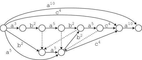
Figure 1: Illustration for the RLE DAWG of $\mathtt{a^{3}b^{2}a^{5}b^{2}a^{5}c^{4}a^{10}}$. The edges in $E$ are represented by the solid arcs, while the suffix links of some nodes are represented by dashed arcs (but their labels are omitted). For simplicity the suffix links of the other nodes are omitted in this figure.

Lemma 5

Given $\mathit{RLE}_{S}$ of any string $S$ where $n=\mathit{size}(\mathit{RLE}_{S})$, $\mathit{RLE\_DAWG}_{S}$ has $O(n)$ nodes and edges, and can be constructed in $O(n\log n)$ time and $O(n)$ extra space in an on-line manner, together with the suffix link set $F$.

Proof

A simple adaptation of the results from [6]. (See Appendix for full proof.)

4.2 On-line LZ factorization using $\mathit{RLE\_DAWG}$

The high-level structure of our on-line algorithm follows that of the off-line algorithm described in the beginning of Section 3.2. In order to find the longest previously occurring prefix of $a_{d-1}^{q}a_{d}^{p_{d}}\cdots a_{n}^{p_{n}}$, which is the next s-factor, we construct the $\mathit{RLE\_DAWG}_{S}$ on-line for the string up to $\mathit{RLE}_{S}[1..d-1]=a_{1}^{p_{1}}a_{2}^{p_{2}}\cdots a_{d-1}^{p_{d-1}}$ and use it, instead of using the $\mathit{RLE\_SA}_{S}$. The difficulty is, as in the off-line case, that only the suffixes that start at a beginning of an RL factor is represented in the $\mathit{RLE\_DAWG}$. Therefore, we again look for the longest previously occurring prefix of $\mathit{RLE}_{S}[d..n]=a_{d}^{p_{d}}\cdots a_{n}^{p_{n}}$ that is immediately preceded by $a_{d-1}^{q}$ in $S$, rather than looking directly for $a_{d-1}^{q}a_{d}^{p_{d}}$ $\cdots$ $a_{n}^{p_{n}}$. We augment the $\mathit{RLE\_DAWG}$ with some more information to make this possible.

Let $E_{[u]}$ denote the set of out-going edges of node $[u]$. For any edge $e=([u],b^{q},[ub^{q}])\in E_{[u]}$ and each character $a\in\Sigma$, define $\mathrm{mpe}_{e}(a)=\max(\{p\mid a^{p}\overleftarrow{u}b^{q}\in\mathit{RLE\_Substr}(S)\}\cup\{0\})$. That is, $\mathrm{mpe}_{e}(a)$ represents the maximum exponent of the RL factor with character $a$, that precedes $\overleftarrow{u}b^{q}$ in $S$.

Lemma 6

Given $\mathit{RLE}_{S}$ of any string $S\in\Sigma^{*}$, $\mathit{RLE\_DAWG}_{S}=(V,E)$, augmented so that $\mathrm{mpe}_{e}(a)$ can be computed in $O(\log\sigma_{S})$ time for any $e\in E$ and any character $a\in\Sigma$, can be constructed in an on-line manner in a total of $O(n\log n)$ time with $O(n)$ space.

Proof

When computing $\mathrm{mpe}_{e}(a)$, consider the following cases: (Case 1) $\overleftarrow{u}b^{q}$ is not the longest member of $[\overleftarrow{u}b^{q}]$, i.e. $\overleftarrow{u}b^{q}\neq\overleftarrow{ub^{q}}$. For any $j\in\mathit{EndPos}(\overleftarrow{u}b^{q})$ let $j^{\prime}=j-\mathit{size}(u)$. We have that $\mathit{RLE}_{S}[j^{\prime}]=a_{j^{\prime}}^{p_{j^{\prime}}}$ where $a_{j^{\prime}}^{p_{j^{\prime}}}\overleftarrow{u}b^{q}\equiv\overleftarrow{u}b^{q}$, i.e., $\overleftarrow{u}b^{q}$ is always immediately preceded by $a_{j^{\prime}}^{p_{j^{\prime}}}$ in $\mathit{RLE}_{S}$. Therefore, $\mathrm{mpe}_{e}(a)=p_{j^{\prime}}$ if $a_{j^{\prime}}=a$ and $0$ otherwise. For any node $[v]\in V$, an arbitrary $j\in\mathit{EndPos}(v)$ can be easily determined in $O(1)$ time when the node is first constructed during the on-line construction of $\mathit{RLE\_DAWG}_{S}$, and does not need to be updated.

(Case 2) $\overleftarrow{u}b^{q}$ is the longest member of $[\overleftarrow{u}b^{q}]$, i.e. $\overleftarrow{u}b^{q}=\overleftarrow{ub^{q}}$. For each occurrence of $a^{p}\overleftarrow{u}b^{q}=a^{p}\overleftarrow{ub^{q}}\in\mathit{RLE\_Substr}(S)$, there must exist a suffix link $([a^{p}\overleftarrow{ub^{q}}],a^{p},[\overleftarrow{ub^{q}}])\in F$. Therefore $\mathrm{mpe}_{e}(a)$ is the maximum of the exponent in the labels of all such incoming suffix links, or $0$ if there are none. By maintaining a balanced binary search tree at every edge $e$, we can retrieve this value for any $a\in\Sigma$ in $O(\log\sigma_{S})$ time. It also follows from the on-line construction algorithm of $\mathit{RLE\_DAWG}_{S}$ that the set of labels of incoming suffix links to a node only increases, and we can update this value in $O(\log\sigma_{S})$ time for each new suffix link. Since $|F|=O(n)$, constructing the balanced binary search trees take a total of $O(n\log\sigma_{S})$ time, and the total space requirement is $O(n)$.

In order to determine which case applies, it is easy to check whether $\overleftarrow{u}b^{q}$ is the longest element of $[\overleftarrow{u}b^{q}]$ in $O(1)$ time by maintaining the length of the longest path to any given node during the on-line construction of $\mathit{RLE\_DAWG}_{S}$. This completes the proof.

Lemma 7

Given $\mathit{RLE}_{S}$ of any string $S\in\Sigma^{*}$, $\mathit{RLE\_DAWG}_{S}=(V,E)$, augmented so that $\max\{p\mid\mathrm{mpe}_{e}(a)\geq q,e=([u],b^{p},[w])\in E_{[u]}\}$ can be computed in $O(\log n)$ time for any $e\in E$, character $a\in\Sigma$, and integer $q\geq 0$, can be constructed in an on-line manner in a total of $O(n\log n)$ time with $O(n)$ space.

Proof

During the on-line construction of the augmented $\mathit{RLE\_DAWG}_{S}$ of Lemma 6, we further construct and maintain a family of PSTs at each node of $\mathit{RLE\_DAWG}_{S}$ with a total size of $O(n)$, containing the information to answer the query in $O(n\log n)$ time. (See Appendix for full proof.)

The next lemma shows how the augmented $\mathit{RLE\_DAWG}_{S}$ can be used to efficiently compute the longest prefix of a given pattern string that appears in string $S$.

Lemma 8

For any pattern string $P\in\Sigma^{*}$, let $\mathit{RLE}_{P}=b_{1}^{q_{1}}b_{2}^{q_{2}}\cdots b_{m}^{q_{m}}$. Given $\mathit{RLE}_{P}$, we can compute the length of the longest prefix $P^{\prime}$ of $P$ that occurs in string $S$ in $O(\mathit{size}(\mathit{RLE}_{P^{\prime}})\log n)$ time, using a data structure of $O(n)$ space, where $n=\mathit{size}(\mathit{RLE}_{S})$.

Proof

Input: $\mathit{RLE\_DAWG}_{S}=(V,E)$, $\mathit{RLE}_{P}=b_{1}^{q_{1}}\cdots b_{m}^{q_{m}}$

1 $h=\max\{q\mid([\varepsilon],b_{1}^{q},[w])\in E_{[\varepsilon]}\}$;

2 if $(m=1)$ or $(h<q_{1})$ then Output $\min(h,q_{1})$ and return ;

3;

4 $\textnormal{{shortcut}}:=\textnormal{{false}}$; $\textnormal{{v}}:=[\varepsilon]$;

5 for $i=2,\ldots,m$ do

6       if $e=(\textnormal{{v}},b_{i}^{q_{i}},[w])\in E_{\textnormal{{v}}}$ and $(\textnormal{{shortcut}}=\textnormal{{true}}~{}~{}\textnormal{{or}}~{}~{}\mathrm{mpe}_{e}(b_{1})\geq q_{1})$ then

             $\textnormal{{v}}:=[w]$; // $\mathit{RLE}_{P}[2..i]\in[w]$

7             if $\mathit{RLE}_{P}[2..i]$ is not the longest element of $[w]$ then $\textnormal{{shortcut}}:=\textnormal{{true}}$ ;

8             ;

9            

10      else

             // $k$:maximum exponent of $b_{i}$ such that $\mathit{val}(b_{1}^{q_{1}}b_{2}^{q_{2}}\cdots b_{i}^{k})\in\mathit{Substr}(S)$.

11             if shortcut = true then $k:=\max\{q\mid(\textnormal{{v}},b_{i}^{q},[w])\in E_{\textnormal{{v}}}\}$;

12             ;

13            else $k:=\max\{q\mid\mathrm{mpe}_{e}(b_{1})\geq q_{1},e=(\textnormal{{v}},b_{i}^{q},[w])\in E_{\textnormal{{v}}}\}$;

14             ;

15             Output $|\mathit{val}(b_{1}^{q_{1}}b_{2}^{q_{2}}\cdots b_{i}^{\min\{q_{i},k\}})|$ and return ;

16            

17      

Output $|P|$ and return; // $P$ itself occurs in $S$

Algorithm 1 Pattern Matching on $\mathit{RLE\_DAWG}_{S}$.

The outline of the procedure is shown in Algorithm 1. First, we check whether the first RL factor $b_{1}^{q_{1}}$ of $P$ is a substring of $S$ (Line 1). If so, the calculation basically proceeds by traversing $\mathit{RLE\_DAWG}_{S}$ with $b_{2}^{q_{2}}b_{3}^{q_{3}}\cdots$ until there is no outgoing edge with $b_{i}^{q_{i}}$ (i.e. $b_{2}^{q_{2}}\cdots b_{i}^{q_{i}}\not\in\mathit{RLE\_Substr}(S)$), or, there is no occurrence of $b_{2}^{q_{2}}\cdots b_{i}^{q_{i}}$ that is immediately preceded by $b_{1}^{q}$, where $q\geq q_{1}$, in $S$. If $\textsf{shortcut}=\textsf{false}$, $b_{2}^{q_{2}}\cdots b_{i}^{q_{i}}$ is the longest element in the node, and the latter check is conduced by the condition $\mathrm{mpe}_{e}(b_{1})\geq q_{1}$. If $\textsf{shortcut}=\textsf{true}$, the character preceding any occurrence of $b_{2}^{q_{2}}\cdots b_{i}^{q_{i}}$ is uniquely determined and already checked in a previous edge traversal, so no further check is required.

By Lemmas 5, 6, and 7, the length of the longest prefix $P^{\prime}$ of $P$ that occurs in $S$ can be computed in $O(\mathit{size}(\mathit{RLE}_{P^{\prime}})(\log n+\log\sigma_{S}))=O(\mathit{size}(\mathit{RLE}_{P^{\prime}})\log n)$ time using a data structure of $O(n)$ space.

Below we give an example for Lemma 8. See Fig. 1 that illustrates $\mathit{RLE\_DAWG}_{S}$ for $\mathit{RLE}_{S}=\mathtt{a^{3}b^{2}a^{5}b^{2}a^{5}c^{4}a^{10}}$, and consider searching string $S$ for pattern $P$ with $\mathit{RLE}_{P}=\mathtt{a^{5}b^{2}a^{7}}$. We start traversing $\mathit{RLE\_DAWG}_{S}$ with the second RL factor $\mathtt{b^{2}}$ of $P$. Since there is an out-going edge labeled $\mathtt{b}^{2}$ from the source node we reach node $v=[\mathtt{b^{2}}]$. There are two suffix links that point to node $v$, $([\mathtt{a^{3}b^{2}}],\mathtt{a^{3}},[\mathtt{b^{2}}])$ and $([\mathtt{a^{5}b^{2}}],\mathtt{a^{5}},[\mathtt{b^{2}}])$. Hence $\mathrm{mpe}_{([\varepsilon],{\mathtt{b^{2}}},[\mathtt{b^{2}}])}(\mathtt{a})=\max\{3,5\}=5$, and thus the prefix $\mathtt{a^{5}b^{2}}$ of $P$ occurs in $S$. We examine whether a longer prefix of $P$ occurs in $S$ by considering the third RL factor $\mathtt{a^{7}}$. There is no out-going edge from $v$ that is labeled $\mathtt{a^{7}}$, hence the longest prefix of $P$ that occurs in $S$ is of the form $\mathtt{a^{5}b^{2}a^{\ell}}$ for some $\ell\geq 0$. We consider the set $E_{v}(\mathtt{a})$ of out-going edges of $v$ that are labeled $\mathtt{a}^{q}$ for some $q$, and obtain $E_{v}(\mathtt{a})=\{([\mathtt{b^{2}}],\mathtt{a^{5}},[\mathtt{b^{2}a^{5}}])\}$. We have $\mathrm{mpe}_{([\mathtt{b^{2}}],\mathtt{a^{5}},[\mathtt{b^{2}a^{5}}])}(\mathtt{a})=\max\{3,5\}=5$ due to the two suffix links pointing to $[\mathtt{b^{2}a^{5}}]$. Thus, the longest prefix of $P$ that occurs in $S$ is $\mathtt{a^{5}b^{2}a^{\min\{7,5\}}}=\mathtt{a^{5}b^{2}a^{5}}$.

Theorem 4.1

Given $\mathit{RLE}_{S}$ for any string $S\in\Sigma^{*}$, the s-factorization of $S$ can be computed in an on-line manner in $O(n\log n)$ time and $O(n)$ extra space, where $\mathit{size}(\mathit{RLE}_{S})=n$.

Proof

Assume the situation described in the first paragraph of Section 3.2. In addition, assume that we have constructed $\mathit{RLE\_DAWG}_{S}^{d-1}$, the $\mathit{RLE\_DAWG}$ (with augmentations described previously) for $\mathit{RLE}_{S}[1..d-1]=a_{1}^{p_{1}}a_{2}^{p_{2}}\cdots a_{d-1}^{p_{d-1}}$. By definition, the longest prefix $P^{\prime}$ of $P=S[\ell..N]$ such that $P^{\prime}\in\mathit{Substr}(\mathit{val}(a_{1}^{p_{1}}a_{2}^{p_{2}}\cdots a_{d-1}^{p_{d-1}}))$, is a prefix of $f_{j}$. By Lemma 8, we can compute $|P^{\prime}|$ in $O(\mathit{size}(\mathit{RLE}_{P^{\prime}})\log d)$ time. A minor technicality is when the longest previous occurrence of $f_{j}$ is self-referencing. This problem can be solved by simply interleaving the traversal and update of $\mathit{RLE\_DAWG}_{S}$ for each RL factor of $f_{j}$. If we suppose that $f_{j}$ spans the RL factors $a_{d}^{p_{d}}\cdots a_{d+g}^{p_{d+g}}$, we can traverse and update $\mathit{RLE\_DAWG}_{S}^{d-1}$ to $\mathit{RLE\_DAWG}_{S}^{d+g}$ in a total of $O(g\log n)$ time by Lemma 7. Thus, totaling for all $f_{j}$, we can compute the s-factorization in $O(n\log n)$ time. $O(n)$ space complexity follows from Lemmas 5, 6, 7, and 8. For any $i>1$, the s-factorization of $\mathit{val}(RLE_{S}[1..i-1])$ and the s-factorization of $\mathit{val}(RLE_{S}[1..i])$ differs only in the last 1 or 2 factors. It is easy to see that the s-factorization of $\mathit{val}(RLE_{S}[1..i])$ is iteratively computed for $i=1,\ldots,n$, and the computation is on-line.

5 Discussion

We proposed off-line and on-line algorithms that compute a well-known variant of LZ factorization, called s-factorization, of a given string $S$ in $O(N+n\log n)$ time using only $O(n)$ extra space, where $N=|S|$ and $n=\mathit{size}(\mathit{RLE}_{S})$. After converting $S$ to $\mathit{RLE}_{S}$ in $O(N)$ time and $O(1)$ extra space (excluding the output), the main part of the algorithms work only on $\mathit{RLE}_{S}$, running in $O(n\log n)$ time and $O(n)$ space, and therefore can be more time and space efficient compared to previous LZ factorization algorithms when the input strings are compressible by RLE. Our algorithms are theoretically significant in that they are the only algorithms which achieve $o(N\log N)$ time using only $o(N)$ extra space for strings with $n=o(N)$, thus offering a substantial improvement to the asymptotic time complexities in calculating the s-factorization, for a non-trivial family of strings. Our algorithms can be easily extended to other variants of LZ factorization. For example, let $m$ be the size of the s-factorization without self-references of a given string. Since Lemma 1 does not hold for s-factorization without self-references, the time complexity of the algorithm is $O(N+(n+m)\log n)$. The working space remains $O(n)$ (excluding the output).

Since conventional string data such as natural language texts are not usually compressible via RLE, the algorithms in this paper, although theoretically interesting, may not be very practical. However, our approach may still have potential practical value for other types of data and objectives. For example, a piece of music can be thought of as being naturally expressed in RLE, where the pitch of the tone is a character, and the duration of the tone is its run length. Other than for the applications to string algorithms [20, 16], mentioned in the Introduction, Lempel Ziv factorization on such RLE compressible strings can be important, due to an interesting application of compression, including LZ77 (gzip), as a measure of distance between data, called Normalized Compression Distance (NCD) [23]. NCD has been shown to be effective for various clustering and classification tasks, including MIDI music data, while not requiring in-depth prior knowledge of the data [12, 19]. The NCD between two strings $S$ and $T$ w.r.t. a compression algorithm basically depends only on the compressed sizes of the strings $S$, $T$, and their concatenation $ST$. Therefore, efficiently computing their s-factorizations from $\mathit{RLE}_{S}$, $\mathit{RLE}_{T}$, and $\mathit{RLE}_{ST}$ would contribute to making the above clustering and classification tasks faster and more space efficient.

Our algorithms are based on RLE variants of classical string data structures. However, our approach does not necessarily make the use of succinct data structures impossible. It would be interesting to explore how succinct data structures can be used in combination with our approach to further improve the space efficiency.

Appendix

This appendix provides complete proofs that were omitted due to lack of space.

Lemma 5. Given $\mathit{RLE}_{S}$ of any string $S$ where $n=\mathit{size}(\mathit{RLE}_{S})$, $\mathit{RLE\_DAWG}_{S}$ has $O(n)$ nodes and edges, and can be constructed in $O(n\log n)$ time and $O(n)$ extra space in an on-line manner, together with the suffix link set $F$.

Proof

The proof is a simple adaptation of the results from [6]. The DAWG of a string of length $m$ has $O(m)$ nodes and edges. Since $\mathit{RLE\_DAWG}_{S}$ is the DAWG of $\mathit{RLE}_{S}$ of length $n$, $\mathit{RLE\_DAWG}_{S}$ clearly has $O(n)$ nodes and edges. If $\sigma$ is the number of distinct characters appearing in $S$, then the DAWG of a string of length $m$ can be constructed in $O(m\log\sigma)$ time and $O(m)$ space, in an on-line manner, using suffix links. Since $|\Sigma_{\mathit{RLE}_{S}}|\leq n$, $\mathit{RLE\_DAWG}_{S}$ with $F$ can be constructed in $O(n\log n)$ time and extra $O(n)$ space, on-line.

Lemma 7. Given $\mathit{RLE}_{S}$ of any string $S\in\Sigma^{*}$, $\mathit{RLE\_DAWG}_{S}=(V,E)$, augmented so that $\max\{p\mid\mathrm{mpe}_{e}(a)\geq q,e=([u],b^{p},[w])\in E_{[u]}\}$ can be computed in $O(\log n)$ time for any $e\in E$, character $a\in\Sigma$, and integer $q\geq 0$, can be constructed in an on-line manner in a total of $O(n\log n)$ time with $O(n)$ space.

Proof

During the on-line construction of the augmented $\mathit{RLE\_DAWG}$ of Lemma 6, we further construct a family of PSTs at each node. Let $T_{u,a,b}$ denote the PST at node $u\in V$ that contains the set of pairs $U_{u,a,b}=\{(q\prime,\mathrm{mpe}_{e}(a))\mid e=([u],b^{q\prime},[w])\in E_{[u]},\mathrm{mpe}_{e}(a)>0\}$, where $a,b\in\Sigma$. By maintaining a two-level balanced binary search tree (a balanced binary search tree inside each node of the first balanced binary search tree) at each node, $T_{u,a,b}$ can be accessed for any $a,b\in\Sigma$ in $O(\log\sigma_{S})$ time. Note that empty PSTs will not be inserted, and hence the total space will be proportional to the number of elements contained in all PSTs. Furthermore, the number of elements in a single PST is bounded by $O(n)$, so $\max\{p\mid\mathrm{mpe}_{e}(a)\geq q,e=([u],b^{p},[w])\in E_{[u]}\}$ can be computed as $\mathit{MaxXInRectangle}(1,|S|,q)$ on $T_{u,a,b}$, in $O(\log n)$ time by Theorem 2.1.

We now bound the total number of elements in all of the PSTs. Recall that $\mathrm{mpe}_{e}(a)=\max(\{p\mid a^{p}\overleftarrow{u}b^{q}\in\mathit{RLE\_Substr}(S)\}\cup\{0\})$.

When a suffix link pointing to a node $[u]$ is created, and when an out-going edge of $[u]$ is created, we must update the PSTs associated with $[u]$. An edge $([u],b^{p},[v])$ is called primary if $\mathit{size}(\overleftarrow{u})+1=\mathit{size}(\overleftarrow{v})$, and is called secondary otherwise.

First, we consider the updates of the PSTs due to the suffix links. Suffix links are created in the following situations (Also refer to [6] for the on-line construction algorithm of DAWGs):

1. The suffix link of the sink node is created.

2. After a node $childState$ is split, then a suffix link from $childState$ to $newChildState$ is created, where $newChildState$ is the new node created by the node split.

Case 1: Let $[v]$ be the node that is pointed by the suffix link of the sink node. Let $e=([u],b^{p},[v])$ be the primary edge to $[v]$, and $a^{q}$ be the RL factor which corresponds to the suffix link. If $q>\mathrm{mpe}_{e}(a)$, then delete the pair $(p,\mathrm{mpe}_{e}(a))$ from the corresponding PST stored in $[u]$, and insert a new pair $(p,q)$ into the PST.

Case 2: There will be no updates in the PSTs. We will discuss the details in Case 3 of edge creation.

Next, we consider the updates of the PSTs due to the edges. Edges are created in the following situations:

1. A primary edge from the old sink $currentSink$ to the new sink $newSink$ is created.

2. A secondary edge to $newSink$ is created.

3. After a node $childState$ is split, then the secondary edge to $childState$ from one of its parents $parentState$ becomes the primary edge from $parentState$ to $newChildState$.

4. After a node $childState$ is split, then all the outgoing edges of $childState$ are copied as the outgoing edges of $newChildState$.

5. After a node $childState$ is split, some secondary edges to $childState$ are redirected and become secondary edges to $newChildState$.

Case 1: Although a new primary edge is created, no pairs are inserted into nor deleted from the PST since there are no suffix links to $newSink$.

Case 2: Let $[u]$ be the node from which a secondary edge to $newSink$ is created. We then insert a pair corresponding to the secondary edge into the PST of $[u]$.

Case 3: In this case, the secondary edge becomes a primary edge. So seemingly we might need to delete the pair corresponding to the existing secondary edge and insert a new pair corresponding to the incoming suffix link. However, both pairs are actually identical, and hence we need no updates in the PSTs.

Case 4: Since the copied edges are all secondary edges (see Fig. 2), similar updates to Case 2 are conducted for all the copied edges.

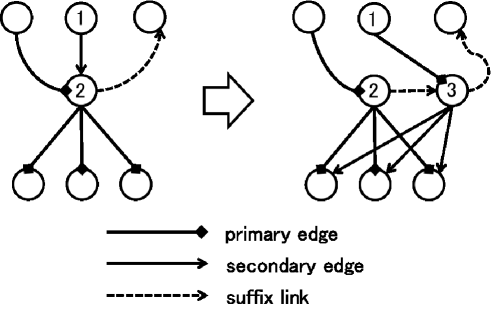
Figure 2: Illustration for node split of the $\mathit{RLE\_DAWG}$ construction algorithm. Node $childState$ (depicted as $\#2$) is split into nodes $childState$ and $newChildState$ (depicted as $\#3$). Note that all the outgoing edges of $newChildState$ are secondary edges.

Case 5: Let $e$ and $e\prime$ be secondary edges before and after redirection, respectively. By the property of the equivalence class, we have that $\mathrm{mpe}_{e}(a)=\mathrm{mpe}_{e\prime}(a)$ for any character $a\in\Sigma$. Hence we need no explicit updates of the PSTs.

By the above discussion, the number of update operations can be bounded by the number of added edges and suffix links. Since the total number of edges and suffix links is $O(n)$, the total number of pairs in all of the PSTs $\sum_{[u]\in V,a,b\in\Sigma}|U_{u,a,b}|$ is also $O(n)$. The total time complexity for the updates is $O(n\log n)$.

References

- [1] Al-Hafeedh, A., Crochemore, M., Ilie, L., Kopylov, J., Smyth, W., Tischler, G., Yusufu, M.: A comparison of index-based Lempel-Ziv LZ77 factorization algorithms. ACM Computing Surveys (in press)
- [2] Amir, A., Landau, G.M., Sokol, D.: Inplace run-length 2d compressed search. TCS 290(3), 1361–1383 (2003)
- [3] Apostolico, A., Erdös, P.L., Jüttner, A.: Parameterized searching with mismatches for run-length encoded strings. TCS (2012)
- [4] Apostolico, A., Landau, G.M., Skiena, S.: Matching for run-length encoded strings. J. Complexity 15(1), 4–16 (1999)
- [5] Arbell, O., Landau, G.M., Mitchell, J.S.: Edit distance of run-length encoded strings. IPL 83(6), 307–314 (2002)
- [6] Blumer, A., Blumer, J., Haussler, D., Ehrenfeucht, A., Chen, M.T., Seiferas, J.: The smallest automaton recognizing the subwords of a text. TCS 40, 31–55 (1985)
- [7] Bunke, H., Csirik, J.: An algorithm for matching run-length coded strings. Computing 50, 297–314 (1993)
- [8] Bunke, H., Csirik, J.: An improved algorithm for computing the edit distance of run length coded strings. IPL 54, 93–96 (1995)
- [9] Chen, G., Puglisi, S., Smyth, W.: Lempel-Ziv factorization using less time & space. Mathematics in Computer Science 1(4), 605–623 (2008)
- [10] Chen, K.Y., Chao, K.M.: A fully compressed algorithm for computing the edit distance of run-length encoded strings. Algorithmica (2011)
- [11] Chen, K.Y., Hsu, P.H., Chao, K.M.: Efficient retrieval of approximate palindromes in a run-length encoded string. TCS 432, 28–37 (2012)
- [12] Cilibrasi, R., Vitányi, P.M.B.: Clustering by compression. IEEE Transactions on Information Theory 51, 1523–1545 (2005)
- [13] Crochemore, M.: Linear searching for a square in a word. Bulletin of the European Association of Theoretical Computer Science 24, 66–72 (1984)
- [14] Crochemore, M., Ilie, L., Iliopoulos, C.S., Kubica, M., Rytter, W., Waleń, T.: LPF computation revisited. In: Proc. IWOCA 2009. pp. 158–169 (2009)
- [15] Crochemore, M., Ilie, L., Smyth, W.F.: A simple algorithm for computing the Lempel Ziv factorization. In: Proc. DCC 2008. pp. 482–488 (2008)
- [16] Duval, J.P., Kolpakov, R., Kucherov, G., Lecroq, T., Lefebvre, A.: Linear-time computation of local periods. TCS 326(1-3), 229–240 (2004)
- [17] Freschi, V., Bogliolo, A.: Longest common subsequence between run-length-encoded strings: a new algorithm with improved parallelism. IPL 90(4), 167–173 (2004)
- [18] Jansson, J., Sadakane, K., Sung, W.K.: Compressed dynamic tries with applications to LZ-compression in sublinear time and space. In: Proc. FSTTCS 2007. pp. 424–435 (2007)
- [19] Keogh, E., Lonardi, S., Ratanamahatana, C.A., Wei, L., Lee, S.H., Handley, J.: Compression-based data mining of sequential data. Data Mining and Knowledge Discovery 14(1), 99–129 (2007)
- [20] Kolpakov, R., Kucherov, G.: Finding maximal repetitions in a word in linear time. In: Proc. FOCS 1999. pp. 596–604 (1999)
- [21] Larsson, N.J., Sadakane, K.: Faster suffix sorting. Tech. Rep. LU-CS-TR:99-214 [LUNFD6/(NFCS-3140)/1–20/(1999)], Dept of Computer Science, Lund University, Sweden (1999)
- [22] Lee, S., Park, K.: Dynamic rank/select structures with applications to run-length encoded texts. TCS 410(43), 4402–4413 (2009)
- [23] Li, M., Chen, X., Li, X., Ma, B., Vitányi, P.M.B.: The similarity metric. IEEE Transactions on Information Theory 50(12), 3250–3264 (2004)
- [24] Liu, J., Huang, G., Wang, Y., Lee, R.: Edit distance for a run-length-encoded string and an uncompressed string. IPL 105(1), 12–16 (2007)
- [25] Liu, J., Wang, Y., Lee, R.: Finding a longest common subsequence between a run-length-encoded string and an uncompressed string. J. Complexity 24(2), 173–184 (2008)
- [26] Mäkinen, V., Ukkonen, E., Navarro, G.: Approximate matching of run-length compressed strings. Algorithmica 35(4), 347–369 (2003)
- [27] Manber, U., Myers, G.: Suffix arrays: A new method for on-line string searches. SIAM J. Computing 22(5), 935–948 (1993)
- [28] McCreight, E.M.: Priority search trees. SIAM J. Comput. 14(2), 257–276 (1985)
- [29] Ohlebusch, E., Gog, S.: Lempel-Ziv factorization revisited. In: Proc. CPM 2011. pp. 15–26 (2011)
- [30] Okanohara, D., Sadakane, K.: An online algorithm for finding the longest previous factors. In: Proc. ESA 2008. pp. 696–707 (2008)
- [31] Starikovskaya, T.: Computing Lempel-Ziv factorization online. In: Proc. MFCS 2012. pp. 789–799 (2012)
- [32] Storer, J., Szymanski, T.: Data compression via textual substitution. Journal of the ACM 29(4), 928–951 (1982)
- [33] Ukkonen, E.: On-line construction of suffix trees. Algorithmica 14(3), 249–260 (1995)
- [34] Weiner, P.: Linear pattern-matching algorithms. In: Proc. of 14th IEEE Ann. Symp. on Switching and Automata Theory. pp. 1–11 (1973)
- [35] Ziv, J., Lempel, A.: A universal algorithm for sequential data compression. IEEE Transactions on Information Theory IT-23(3), 337–343 (1977)
- [36] Ziv, J., Lempel, A.: Compression of individual sequences via variable-length coding. IEEE Transactions on Information Theory 24(5), 530–536 (1978)