Multi-physics simulations using a hierarchical interchangeable software interface

Abstract

We introduce a general-purpose framework for interconnecting scientific simulation programs using a homogeneous, unified interface. Our framework is intrinsically parallel, and conveniently separates all component numerical modules in memory. This strict separation allows automatic unit conversion, distributed execution of modules on different cores within a cluster or grid, and orderly recovery from errors. The framework can be efficiently implemented and incurs an acceptable overhead. In practice, we measure the time spent in the framework to be less than 1% of the wall-clock time. Due to the unified structure of the interface, incorporating multiple modules addressing the same physics in different ways is relatively straightforward. Different modules may be advanced serially or in parallel. Despite initial concerns, we have encountered relatively few problems with this strict separation between modules, and the results of our simulations are consistent with earlier results using more traditional monolithic approaches. This framework provides a platform to combine existing simulation codes or develop new physical solver codes within a rich “ecosystem” of interchangeable modules.

1 Introduction

Large-scale, high-resolution computer simulations dominate many areas of theoretical and computational science. The demand for such simulations has expanded steadily over the past decade, and is likely to continue to grow in coming years due to the increase in the volume, precision, and dynamic range of experimental data, as well as the widening spectral coverage of observations and laboratory experiments. Simulations are often used to mine and understand large observational and experimental datasets, and the quality of these simulations must keep pace with the increasingly high quality of experimental data.

In our own specialized discipline of computational astrophysics, numerical simulations have increased dramatically in both scope and scale over the past four decades. In the 1970s and 1980s, large-scale astrophysical simulations generally incorporated “mono-physics” solutions—in our case, the sub-disciplines of stellar evolution [1], gas dynamics [2], and gravitational dynamics [3]. A decade later, it became common to study phenomena combining a few different physics solvers [4]. Today’s simulation environments incorporate multiple physical domains, and their nominal dynamic range often exceeds the standard numerical precision of available compilers and hardware [3].

Recent developments in hardware—in particular the rapidly increasing availability of multi-core architectures—have led to a surge in computer performance [5]. With the volume and quality of experimental data continuously improving, simulations expanding in scope and scale, and raw computational speed growing more rapidly than ever before, one might expect commensurate returns in the scientific results returned. However, a major bottleneck in modern computer modeling lies in the software, the growing complexity of which is evident in the increase in the number of code lines, the lengthening lists of input parameters, the number of underlying (and often undocumented) assumptions, and the expanding range of initial and boundary conditions.

Simulation environments have grown substantially in recent years by incorporating more detailed interactions among constituent systems, resulting in the need to incorporate very different physical solvers into the simulations, but the fundamental design of the underlying codes has remained largely unchanged since the introduction of object-oriented programming [6] and patterns [7]. As a result, maintaining and extending existing large-scale, multi-physics solvers has become a major undertaking. The legacy of design choices made long ago can hamper further development and expansion of a code, prevent scaling on large parallel computers, and render maintenance almost impossible. Even configuring, compiling, and running such a code has become a complex endeavor, not for the faint of heart. It has become increasingly difficult to reproduce simulation results, and independent code verification and validation are rarely performed, even though all researchers agree that computer experiments require the same degree of reproducibility as is customary in laboratory settings.

We suggest that the root cause of much of this code complexity lies in the traditional approach to incorporating multi-physics components into a simulation—namely, solving the equations appropriate to all components in a single monolithic software suite, often written by a single researcher or research group. Such a solution may seem desirable from the standpoint of consistency and performance, but the resulting software generally suffers from all of the fundamental problems just described. In addition, integration of new components often requires sweeping redesign and redevelopment of the code. Writing a general multi-physics application from scratch is a major undertaking, and the stringent requirements of high-quality, fault-tolerant scientific simulation software render such code development by a single author almost impossible.

But why reinvent or re-engineer a monolithic suite of coupled mono-physics solvers when well-tested applications already exist to perform many or all of the necessary individual tasks? In many scientific communities there is a rich tradition of sharing scientific software. Many of these programs have been written by experts who have spent careers developing these codes and using them to conduct a wide range of numerical experiments. These packages are generally developed and maintained independently of one another. We refer to them collectively as “community” software. The term is intended to encompass both “legacy” codes that are still maintained but are no longer under active development, and new codes still under development to address physical problems of current interest. Together, community codes represent an invaluable, if incoherent, resource for computational science.

Coupling community codes raises new issues not found in monolithic applications. Aside from the wide range of physical processes, underlying equations, and numerical solvers they represent, these independent codes generally also employ a wide variety of units, input and output methods, file formats, numerical assumptions, and boundary conditions. Their originality and independence are strengths, but the lack of uniformity can also significantly reduce the “shelf life” of the software. In addition, directly coupling the very dissimilar algorithms and data representations used in different community codes can be a difficult task—almost as complex as rewriting the codes themselves. But whatever the internal workings of the codes, they are designed to represent a given domain of physics, and different codes may (and do in practice) implement alternate descriptions of the same physical processes. This suggests that integrating community codes should be possible using interfaces based on physical principles.

In this paper we present a comprehensive solution to many of the problems mentioned above, in the form of a software framework that combines remote function calls with physically based interfaces, and implements an object oriented data model, automatic conversion of units, and a state handling model for the component solvers, including error recovery mechanisms. Communication between the various solvers is realized via a centralized message passing framework, under the overall control of a high-level user interface. In §2, we name our framework MUSE, the MUlti-physics Software Environment. An example of the MUSE framework is presented in §3. In §4 we describe a production implementation of AMUSE, the astrophysics MUSE environment, which supports a wide range of programming languages and physical environments.

1.1 An historical perspective on MUSE

The basic concepts of MUSE are rooted in the earliest development of multi-scale software in computational astrophysics. The idea of combining codes within a flexible framework began with the NEMO project in 1986 at the Institute for Advanced Study (IAS) in Princeton [8, 9]. NEMO was (and still is) aimed primarily at collisionless galactic dynamics. It used a uniform file structure to communicate data among its component programs.

The Starlab package [10, 11], begun in 1993 (again at IAS), adopted the NEMO toolbox approach, but used pipes instead of files for communication among modules. The goal of the project was to combine dynamics and stellar and binary evolution for studies of collisional systems, such as star clusters. The stellar/binary evolution code SeBa [12] was combined with a high-performance gravitational stellar dynamics simulator. Because of the heterogeneous nature of the data, not all tools were aware of all data types (for example, the stellar evolution tools generally had no inherent knowledge of large-scale gravitational dynamics). As a result, the package used an XML-like tagged data format to ensure that no information was lost in the production pipeline—unknown particle data were simply passed unchanged from input to output.

The intellectual parent of (A)MUSE is the MODEST initiative, begun in 2002 at a workshop at the American Museum of Natural History in New York. The goal of that workshop was to formalize some of the ideas of modular software frameworks then circulating in the community into a coherent system for simulating dense stellar systems. Originally, MODEST stood for MOdeling DEnse STellar systems (star clusters and galactic nuclei). The name was later expanded, at the suggestion of Giampolo Piotto (Padova) to Modeling and Observing DEnse STellar systems. The MODEST web page can be found at http://www.manybody.org/modest. Since then, MODEST has gone on to provide a lively and long-lived forum for discussion of many topics in astrophysics. (A)MUSE is in many ways the software component of the MODEST community. An early example of MUSE-like code can be found in the proceedings of the MODEST-1 meeting [13].

Subsequent MODEST meetings discussed many new ideas for modular multiphysics applications [e.g. 14]. The basic MUSE architecture, as described in this paper, was conceived during the 2005 MODEST-6a workshop in Lund [Sweden, 15]. The MUSE name, and the first lines of MUSE code, were created during MODEST-6e in Amsterdam in 2006, and expanded upon over the next 1–2 years. The “Noah’s Ark” milestone (meeting our initial goal of having two independent modules for solving each particular type of physics) was realized in 2007, during MODEST-7f in Amsterdam and MODEST-7a in Split [Croatia 16]. The AMUSE project, short for for Astrophysics Multi-Purpose Software Environment, a re-engineered version of MUSE—“MUSE 2.0,” building on the lessons learned during the previous 3 years—began at Leiden Observatory in 2009.

2 The MUSE framework

Each of the problems discussed in §1 could in principle be addressed by designing an entirely new suite of programs from scratch. However, this idealized approach fails to capitalize on the existing strengths of the field by ignoring the wealth of highly capable scientific software that has been developed over the last four or five decades. We will argue that it is more practical, and considerably easier, to introduce a generalized interface that connects existing solvers to a homogeneous and easily extensible framework.

At first sight, the approach of assimilating existing software into a larger framework would appear to be a difficult undertaking, particularly since community software may be written in a wide variety of languages, such as FORTRAN, C, and C++, and exhibits an enormous diversity of internal units and data structures. On the other hand, such a framework, if properly designed, could be relatively easy to use, since learning one simulation package is considerably easier than mastering the idiosyncrasies of many separate programs. The use of standard calling procedures can enable even novice researchers quickly to become acquainted with the environment, and to perform relatively complicated simulations using it.

To this end, we propose the Multi-physics Software Environment, or MUSE. Within MUSE, a user writes a relatively simple script with a standardized calling sequence to each of the underlying community codes. Instructions are communicated through a message-passing interface to any of a number of spawned community modules, which respond by performing operations and transferring data back through the interface to the user script.

As illustrated in Fig. 1, the two top-level components of MUSE:

• The user script, which implements a specific physical problem or set of problems, in the form of system-provided or user-written scripts that serve as the user interface onto the MUSE framework. The coupling between community codes is implemented in this layer, with the help of support classes provided by the manager.

• The community module, comprising three key elements:

  1. The manager, which provides an object-oriented interface onto the communication layer via a suite of system-provided utility functions. This layer handles unit conversion, as discussed below, and also contains the state engine and the associated data repository, both of which are required to guarantee consistency of data across modules. The role of this layer is generic—it is not specific to any particular problem or to any single physical domain. In §4.1 we discuss an actual implementation of the manager for astrophysical problems.

  2. The communication layer, which realizes the bi-directional communication between the manager and the community code layer. This is implemented via a proxy and an associated partner, which together provide the connection to the community code.

  3. The community code layer, which contains the actual community codes and implements control and data management operations on them. Each piece of code in this layer is domain-specific, although the code may be designed to be very general within its particular physical domain.

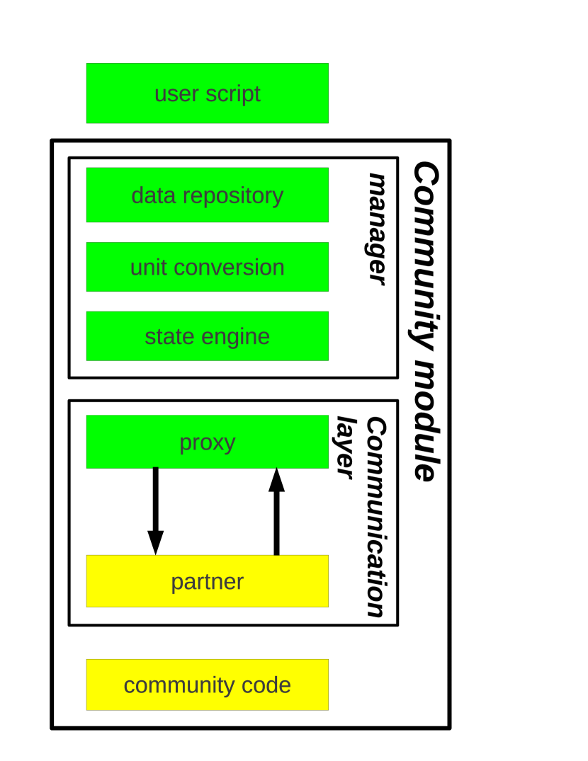
Figure 1: The MUSE framework architecture is based on a three-layered design. The top layer consists of a user script written by the end-user in python (top box). The manager is part of the community module and consists of a data repository, unit conversion, and a state engine. The community module also includes the partner-proxy pair in the communication layer—a bi-directional message passing framework—and a community code (bottom box).

2.1 Choice of programming languages

We have adopted python as the implementation language for the MUSE framework and high-level management functions, including the bindings to the communication interface. This choice is motivated by python’s broad acceptance in the scientific community, its object oriented design, and its ability to allow rapid prototyping, which shortens the software development cycle and enables easy access to the community code in the community module, albeit at the cost of slightly reduced performance. However, the entire MUSE framework is organized in such a way that relatively little computer time is actually spent in the framework itself, as most time is spent in the community code. The overhead from python compared to a compiled high-level language is $\,{\raise-2.15277pt\hbox{$\buildrel<\over{\sim}$}}\ 10$%, and often much less (see §5).

As discussed further in §2.2.2, our implementation of the communication layer in MUSE uses the standard Message Passing Interface protocol [17], although we also have an operational implementation using SmartSockets [18] via the Ibis framework [19, 20] (see [21] for an actual implementation). Normally MPI is used for communication between compute nodes on parallel distributed-memory systems. However, here it is used as the communication channel between all processes, whether or not they reside on the same node as the control script, and whether or not they are themselves parallel. The proxy side of the message-passing framework in the communication layer is implemented in python, but the partner side is normally written in the language used in the community code. Thus our only real restriction on supported languages is the requirement that the community code is written in a language with standard MPI bindings, such as C, C++, or a member of the FORTRAN family.

2.2 The community module

The community module consists of the actual community code and the bi-directional communication layer enabling low-level MPI communication between the proxy and the partner. Each community module contains a python class of functions dedicated to communication with the community code. Direct use of this low-level class from within a user script is not trivial, because it requires considerable replication of code dealing with data models, unit conversion, and exception handling, and is discouraged. Instead, the MUSE framework provides the manager layer above the community module layer to manage the bookkeeping needed to maintain the interface with the low-level class.

2.2.1 The community code

Community applications may be programmed in any computer language that has bindings to the MPI protocol. In practice, these codes exhibit a wide variety of structural properties, model diverse physical domains, and span broad ranges of temporal and spatial scales. In our astrophysical AMUSE implementation (see §4.1), this diversity is exemplified by a suite of community programs ranging from toy codes to production-quality high-precision dedicated solvers. A user script can be developed quickly using toy codes until the production and data analysis pipelines are fully developed, then easily switched to production quality implementations of the physical solvers for actual large-scale simulations.

In principle, each of the community modules can be used stand alone, but the main strength of MUSE is in the coupling between them. Many of the codes incorporated in our practical implementation are not written by us, but are publicly available and are amply described in the literature.

2.2.2 The communication layer

Bi-directional communication between a running community process and the manager can in principle be realized using any protocol for remote interprocess communication. Our main reasons for choosing MPI are similar to those for adopting python—widespread acceptance in the computational science community and broad support in many programming languages and on most computing platforms.

The communication layer consists of two main parts, a python proxy on the manager side of the framework and a partner on the community code side. The proxy converts python commands into MPI messages, transmits them to the partner, then waits for a response. The partner waits for and decodes MPI messages from the proxy into community code commands, executes them, then sends a reply. The MPI interface allows the user script and community modules to operate asynchronously and independently. As a practical matter, the detailed coding, decoding, and communications operations in the proxy and the partner are never hand-coded. Rather, they are automatically generated as part of the MUSE build process, from a high-level python description of the community module interface.

We note that other solutions to linking high-level languages within python exist—e.g. swig and f2py, and in fact both were used in earlier implementations of the MUSE framework [16]. However, despite their generality, these solutions cannot maintain name space independence between community modules, and in addition are incapable of accommodating high-performance parallel community codes. For these reasons, we have abandoned the standard solutions in favor of our customized, high-performance MPI alternative.

The use of MPI may seem like overkill in the case of serial operation on a single computing node (as might well be the case), but it imposes negligible overhead, and even here it offers significant practical advantages. It rigorously separates all community processes in memory, guaranteeing that multiple instances of a community module are independent and explicitly avoiding name space conflicts. It also ensures that the framework remains thread-safe when using older community codes that may not have been written with that concept in mind.

Despite the initial threshold for its implementation and use, the relative simplicity of the message-passing framework allows us to easily couple multiple independent community codes as community modules, or multiple copies of the same community module, if desired (see Fig. 1). An example of the latter might be to simulate simultaneously two separate objects of the same type, or the same physics on different scales, or with different boundary conditions, without having to modify the data structures in the community code.

As a bonus, the framework naturally accommodates inherently parallel community modules and allows simultaneous execution of independent modules from the user script. Individual community modules can be offloaded to other processors, in a cluster or on the grid, and can be run concurrently without requiring any changes in the user script. This makes the MUSE framework well suited for distributed computing with a wide diversity of hardware architectures (see §5).

2.2.3 The manager

Between the user script and the communication layer we introduce the manager, part of the community module. This part of the code is visible to the script-writing user and guarantees that all accessible data are up to date, have the proper format, and are expressed in the correct units.

The manager layer constructs data models (such as particle sets or tessellated grids) on top of all functions in the low-level communication class and checks the error codes they return. To allow different modules to work in their preferred systems of units, the manager incorporates a unit transformation protocol (see §2.4). It also includes a state engine to ensure that functions are called in a controlled way, as many community codes are written with specific assumptions about calling procedures. In addition, a data repository is introduced to guarantee that at least one self-consistent copy of the simulation data always exists at any given time. This repository can be structured in one or more native formats, such as particles, grids, tessellation, etc, depending on the topology of the data adopted in the community code.

Each community code has its own internal data, needed for modeling operations but not routinely exposed to the user script. However, some of these data may be needed by other parts of the framework. To share data effectively, and to minimize the bookkeeping required to manage data coherency, the most fundamental parts of the community data are replicated in the structured repository in the manager. The internal data structures differ, but the repository imposes a standard format. The repository allows the user to access community module data from the user script without having to make individual (and often idiosyncratic) calls to individual community modules. The repository is updated from the community module on demand, and is considered to be authoritative within the script.

The separation of the manager from the community module realizes a flexibility that allows the user to swap modules and recompute the same problem using different physics solvers, providing an independent check of the implementation, validation of the model, and verification of the results, simply by rerunning the same initial state using another community module. Potentially even more interesting is the possibility of solving some parts of a problem with one solver and others with a different solver of the same type, combining the results at a later stage to complete the solution. While studying the general behavior of a simulation, perhaps to test a hypothesis or guide our physical intuition, we may elect to use computationally cheaper physics solvers, then switch to more robust, but computationally more expensive, modules in a production run. Alternatively, we might choose adopt less accurate solvers for physical domains that are not deemed crucial to capturing the correct overall behavior.

Another advantage of separating of the manager from the community module is the possibility of combining existing community modules into new community modules which can themselves be coupled via the manager, building a hierarchical environment for simulating complex physical systems with multiple components.

2.3 The user script

The MUSE framework is controlled by the user via python scripts (see §3 and §4.1). The main tasks of these scripts are to identify and spawn community modules, control their calling sequences, and manage the data flow among them. The user script and the spawned community code are connected by a communication channel embedded in the community module and maintained by the manager. Since the community modules do not communicate directly with one another, the only communication channels are between modules and the user script. The number of community modules controlled by a user script is effectively unlimited, and multiple instances of identical modules can be spawned.

The main objective of the user script is to read in or generate an input model, process these initial conditions through one or more simulation modules, and subsequently mine and analyze the resultant data. In practice the user script will itself be composed of a series of scripts, each performing one specific functionality.

2.4 Inter-module data transfer and unit conversion

Computer scientists tend to attribute types to parameters and variables, and generally impose strict rules for the conversion from one type to another. In physics, data types are almost never important, but units are crucial for validating and checking the consistency of a calculation or simulation. The lack of coherent unit handling in programming environments is notorious, and can cause significant problems in multi-physics simulations, particularly for inexperienced researchers.

In many cases, a researcher can define a set of dimensionless variables applicable to a specific simulation, within the confines of a set of rather strict assumptions. For a mono-physics simulation, the consistent use of such variables is generally clear to most users. However, as soon as an expert from another field attempts to interpret the results, or when the output of one simulation is used by another program, units must be restored and the data converted to another physical system for further processing and interpretation.

The absence of units in scientific software raises two important problems. The first is the loss of an independent consistency check for theoretical calculations. The second is the expert knowledge and intuition required to manage dimensionless variables or otherwise unfamiliar units. Few would recognize $4.303\times 10^{43}$ as the radius of the Sun in units of the Planck length, even though it is not completely inconceivable that an astronomer might use such units in a simulation. To address these issues, MUSE incorporates a unit-conversion module as part of the manager (see § 2.2.3) to guarantee that all communications within the top-level user script are performed in the proper units. In order to prevent unit checking and conversion from becoming a performance bottleneck, we adopt lazy evaluation, performing unit conversion only when explicitly required.

3 A simple implementation

The above description of MUSE is somewhat abstract. Here we present a simple example—the calculation of the orbital period of a binary star in a circular orbit. This is a straightforward astrophysical calculation that serves to illustrate the basic operation of the framework. The community code that calculates the orbital period is presented in Fig. 2.

[8] #include ”community.h” #include ”math.h”

int orbital_period(double orbital_separation, double total_mass, double *orbital_period) if (total_mass ¡= 0.0) return -1; *orbital_period = sqrt(pow(orbital_separation, 3.)/total_mass) ; return 0; [8]

Figure 2: The community code.

The partner requires the definitions of all interface functions in the community code, which are included from the community.h header file, presented in Fig. 3. (Note that, as mentioned earlier, in a practical implementation the communication code is actually machine generated. The code here is hand-written, for purposes of exposition.)

[8] int orbital_period(double orbital_separation, double total_mass, double *orbital_period);

Figure 3: The community header file.

The user script that initializes the required parameters (orbital separation, total mass of the binary) and computes the orbital period is presented in Fig. 4. Because of the simplicity of this example we do not include unit conversion here; we tacitly assume that the total binary mass is in units of the mass of the sun, and the orbital separation in astronomical units; the average orbital separation of Earth around the Sun. The output orbital period is expressed in years. This example illustrates how a set of units can be convenient within the implicit choices of a community code, but counterintuitive for researchers from other disciplines. Calls to the community code are initiated by the user script, sent to the proxy, received by the partner, and executed by the community code. The interaction between these MUSE components is illustrated in Fig. 5.

[8] import proxy from optparse import OptionParser

def new_option_parser(): arguments = OptionParser() arguments.add_option(”-a”, dest=”a”,type=”float”,default=1.0) arguments.add_option(”-M”, dest=”M”,type=”float”,default=1.0) return arguments

def main(a=1.0, M=1.0) : community_code = proxy.CodeProxy() print ”Orbital period: ”, community_code.orbital_period(a, M), ” years” community_code.stop()

if __name__== ’__main__’: arguments, options = new_option_parser().parse_args() main(**arguments.__dict__)

Figure 4: the main user script.

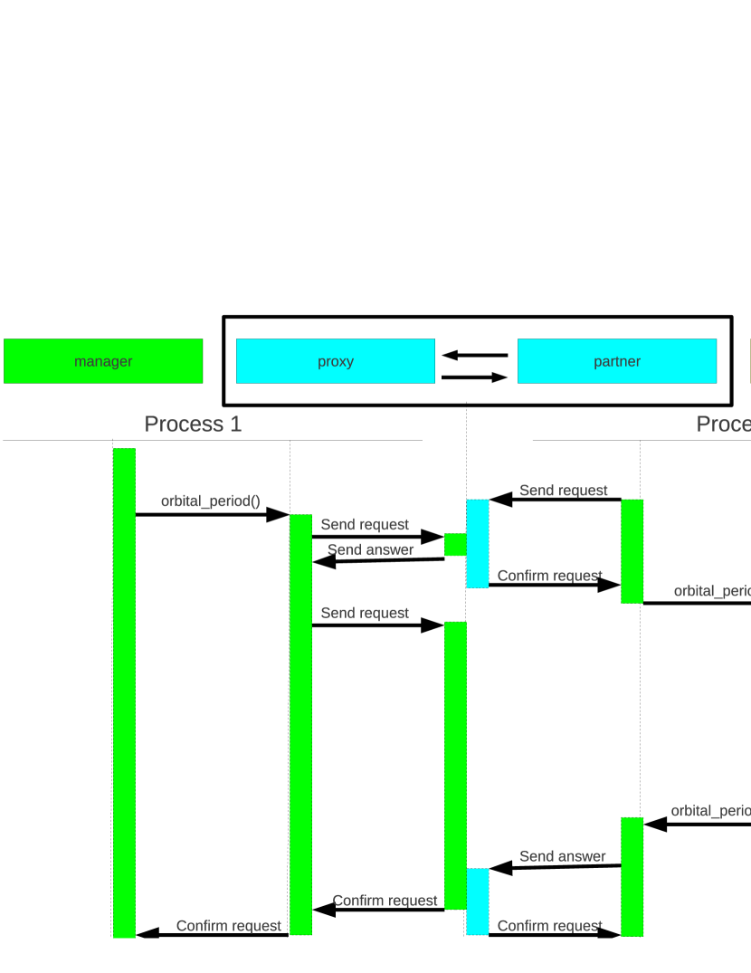
Figure 5: The MUSE framework manages the interaction between the user script (left) and the community code (right). When the script is started, process 1 spawns the community code and message-passing partner as process 2. Process 2 starts by sending a request for instructions, and then waits. At some later time the user script requests the execution of the function orbital_period(). This results in a request to the communication layer. Since process 2 already has an open request both processes return with the confirmation that the request is satisfied. Process 1 subsequently sends a new request to return the resulting data and a confirmation that the function orbital_period() has been executed correctly. In the mean time process 2 executes the function, returning the requested data and a message to the framework once the execution is complete.

The python class proxy takes care of setting up the community code, encoding the arguments, sending the message, and decoding the results. In an actual MUSE implementation the proxy is split into two parts, one to translate the arguments into a generic message object (and translate the returned message into return parameters), and one to send the message using the communication library (MPI). The source code listing in Fig. 6 presents a working example of a proxy.

[8] from mpi4py import MPI import numpy

class CodeProxy(object): def __init__(self): self.intercomm = MPI.COMM_SELF.Spawn(’./community_code’)

def send_function_id(self, function_id): self.intercomm.Send([function_id, MPI.CHARACTER], tag=997)

def send_arguments(self, arguments): self.intercomm.Send([arguments, MPI.DOUBLE], tag=998)

def recv_error_message(self): errorcode_array = numpy.empty(1, dtype=’int32’) self.intercomm.Recv([errorcode_array, MPI.INT], tag = 999) errorcode = errorcode_array[0]

if errorcode == -1000: raise Exception(”Unknown function id received by partner”) elif errorcode ¡ 0: raise Exception(”Partner, errorcode is 0”.format(errorcode))

def recv_answer(self, number_of_answers = 1): answer_array = numpy.empty(number_of_answers, dtype=’float64’) self.intercomm.Recv([answer_array, MPI.DOUBLE], tag = 996) return answer_array

def orbital_period(self, orbital_separation, total_mass): arguments = numpy.array([orbital_separation, total_mass]) self.send_function_id(’P’) self.send_arguments(arguments) self.recv_error_message() answer = self.recv_answer(1) return answer[0]

def stop(self): self.send_function_id(’q’) self.recv_error_message() self.intercomm.Disconnect() [8]

Figure 6: The proxy part of the community module.

Messages sent via MPI are received by the partner code, which decodes them and executes the actual function calls in the community code. Subsequently it encodes and returns the results in a message to the proxy. The partner code is generally written in the same language as the community code, in this case C++. In the source code listing in Fig. 7 we present a working example of a partner. Fig. 5 and the associated source listing Fig. 7 might seem at first glance to be a rather complicated way to perform some rather simple message passing. However, this procedure allows us to encapsulate existing code, rendering it largely independent of the rest of the framework, allowing the implementation of parallel internal architecture, and opening the possibility of launching a particular application on a remote computer. Also, if one of these encapsulated codes stops prematurely, the framework remains operational, and simply detects the unscheduled termination of a particular application. A complete crash of one of the community modules, however, will likely still cause the framework to break.

[8] #include ”community.h” #include ”mpi.h” #include ¡mpi.h¿

void event_loop() MPI::Intercomm intercomm = MPI::COMM_WORLD.Get_parent(); int rank = MPI::COMM_WORLD.Get_rank(); bool continue_run = true;

while (continue_run) char function_id; int errorcode = 0; intercomm.Recv(&function_id, 1, MPI::CHARACTER, 0, 997);

switch (function_id) case ’P’: double args[2]; double answer; intercomm.Recv(args, 2, MPI::DOUBLE, 0, 998); errorcode = orbital_period(args[0], args[1], answer); if (rank == 0) intercomm.Send(errorcode, 1, MPI::INT, 0, 999); if(errorcode == 0) intercomm.Send(answer, 1, MPI::DOUBLE, 0, 996); break; case ’q’: intercomm.Send(errorcode, 1, MPI::INT, 0, 999); intercomm.Disconnect(); continue_run = false; break; default: errorcode = -1000; intercomm.Send(errorcode, 1, MPI::INT, 0, 999); break;

int main(int argc, char *argv[]) MPI::Init(argc, argv); event_loop(); MPI::Finalize();

Figure 7: The partner part of the community module.

4 Advanced MUSE

The simple example described in §3 does not demonstrate the full potential of a MUSE framework, and specifically the wide range of possibilities that arise from coupling community codes.

Many problems in astrophysics encompass a wide variety of physics. As a practical demonstration of MUSE, we present here an open-source production environment in an astrophysics context, implemented by coupling community codes designed for gravitational dynamics, stellar evolution, hydrodynamics, and radiative transfer, the most common physical domains encountered in astrophysical simulations. We call this implementation AMUSE, the Astrophysics MUltiphysics Software Environment [22, 23].

4.1 AMUSE: a MUSE implementation for astrophysics

AMUSE is a complete implementation of MUSE, with a fully functional interface including automated unit conversion, a structured data repository (see §2.2.3), multi-stepping via operator splitting (see §4.3.1), and (limited) ability to recover from fatal errors (see §4.2). A wide variety of community codes is available, including multiple modules for each of the core domains listed above, and the framework is currently used in a variety of production simulations. AMUSE is designed for use by researchers in many fields of astrophysics, targeted at a wide variety of problems, but it is currently also used for educational purposes, in particular for training MSc. and Ph.D. students.

The development of a MUSE sprang from our desire to simulate a multi-physics system within a single conceptual framework. The fundamental design stems from our earlier endeavour in the development of the starlab software environment [10] in which we combined stellar evolution and gravitational dynamics. The drawback with starlab was rigid coupling between domains, which made the framework inflexible and less applicable than desired to a wider range of practical problems. The AMUSE framework provides us with a general solution to the problem, allowing us to hierarchically combine numerical solvers within a single environment to create new and more capable community modules. Examples in AMUSE include coupling a direct N-body algorithm with a hierarchical tree-code, and combining a smoothed-particle hydrodynamics solver with a larger-scale grid-based hydrodynamics solver.

Such dynamic coupling has practical applications in resolving short time scale shocks using a grid-based hydrodynamics solver within a low-resolution smoothed-particles hydrodynamics environment, or in changing the evolutionary prescription of a star at run-time—for example when two stars collide and the standard “lookup” description of their evolution must be replaced by “live” integration of the merger product. The validation and verification of coupled solvers remain a delicate issue. It may well be that the effective strength of the coupling can only be determined at run-time, and it may require a thorough study for each application to identify the range of parameters within which the coupled solver can be applied.

Adding new community modules is straightforward. The environment runs efficiently on a single PC, on multi-core architectures, on supercomputers, and on distributed computers [21]. Given our experience with AMUSE, we are confident that it can be relatively easily adapted as the basis for a MUSE implementation in another research field, coupling a different suite of numerical solvers. The AMUSE source code is freely available from the AMUSE website.

We have applied AMUSE to a number of interesting problems incorporating stellar evolution and gravitational dynamics [24, 25], and to the combination of stellar evolution and the dynamics of stars and gas [26]. The former reference provides an explanation for the formation of the binary millisecond pulsar J1903+0327; the latter explores the consequences of early mass loss from stars in young star clusters by means of stellar winds and supernovae. In Fig. 8 we present three-dimensional renderings of several snapshots of the latter calculation.

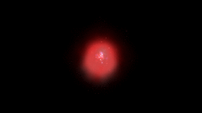
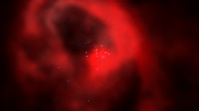
Figure 8: Computer rendering of a simulation of a star cluster (1000 stars with a Salpeter mass function [27] distributed in a 1 pc Plummer sphere [28]) in which the mutual gravity and movement of the stars were solved self-consistently with the evolution of the stars and the hydrodynamics of the protostellar gas, together with the stellar outflow in winds and supernovae [26]. The top image presents the stars and the gas distribution at the birth of the cluster, the second image at an age of about 4 Myr, and the bottom image at about 8 Myr, just before the last residual gas is blown out by the first supernova explosion. This 3D visualization is created by Maarten van Meersbergen and the animation can be downloaded from http://www.cs.vu.nl/ibis/demos.html [21].

4.2 Failure recovery

Real-world simulation codes crash. Crashes are inevitable, but restarting and continuing a simulation afterwards can be a very delicate procedure, and there is a fine line between science and nonsense in the resulting data. In many cases catastrophic failure is caused by numerical instabilities that are either not understood, in which case a researcher would like to study them further, or are part of a natural phenomenon that cannot be modeled in sufficient detail by the current community code. Recognizing and understanding code failure is a time consuming but essential part of the gritty reality of working with simulation environments.

In many cases, simulation codes are developed with the implicit assumption that a user has some level of expert knowledge, in lieu of providing user-friendly error messages, debugging assistance, and exception handling. However, for a framework like AMUSE, such an assumption may pose problems for the run-time behavior and stability of the system, as well as being confusing and frustrating for the user.

To some degree, code fatalities can be handled gracefully by the MUSE manager. The failure of a particular community module does not necessarily result in the failure of the entire framework. As a response, the framework can return a meaningful error message, or, more usefully, continuing the simulation using another community code written for the same problem. The approach is analogous to fault-tolerant computing, in which a management process detects node failure and redirects the processes running on the failed node.

4.3 Code coupling strategies

In the AMUSE framework we recognize six distinct strategies for coupling community modules. Some can be programmed easily by hand, although they can be labour intensive, while others are enabled by our implementation of the AMUSE framework. The examples presented below are drawn taken from the public version of AMUSE.

1 Input/Output coupling:

The loosest type of coupling occurs when the result of code A generates the initial conditions for code B. For example, a Henyey stellar evolution code might generate mass, density and temperature profiles for a subsequent 3-dimensional hydrodynamical representation of a star.

2 One-way coupling:

System A interacts with (sub)system B, but the back-coupling from B to A is negligible. For example, stellar mass loss due to internal nuclear evolution is often important for the global dynamics of a star cluster, but the dynamics of the cluster usually does not affect the evolution of individual stars (except in the rare case of an physical stellar collision).

3 Hierarchical coupling:

Subsystems A1 and A2 (and possibly more) are embedded in parent system B, which affects their evolution, but the subsystems do not affect the parent or each other. For example, the evolution of cometary Oort clouds are strongly influenced by, but are irrelevant to, the larger galactic potential.

4 Serial coupling:

A system evolves through distinct regimes which need different codes A, B, C, etc., applied subsequently in an interleaved way, to model them. For example, a collision between two stars in a dense star cluster may be resolved using one or more specialized hydrodynamics solvers, after which the collision product is reinserted into the gravitational dynamics code.

5 Interaction coupling:

This type of coupling occurs when there is neither a clear temporal or spatial separation between systems A and B. For example, in the interaction between the interstellar medium and the gravitational dynamics of an embedded star cluster, both the stellar and the gas dynamics must incorporate the combined gravitational potential of the gas and the stars.

6 Intrinsic coupling:

This may occur where the physics of the problem necessitates a solver that encompasses several types of physics simultaneously, and does not allow for temporal or spatial separation. An example is magnetohydrodynamics, where the gas dynamics and the electrodynamics are so tightly coupled that they cannot be separated.

With the exception of the last, all types of coupling can be efficiently implemented in AMUSE using single-component solvers. Many of the coupling strategies are straightforward in AMUSE, with the exception of the interaction and intrinsic coupling types. For interaction coupling, the symplectic multi-physics time-stepping approach originally described in [29] usually works very well. For intricate intrinsic coupled codes it may still be more efficient to write a monolithic framework in a single language, rather than adopt the method proposed here.

4.3.1 Multi-physics time stepping by operator splitting

The relative independence of the various community modules in AMUSE allows us to combine them in the user script by calling them consecutively. This is adequate for many applications, but in other situations such rigid time stepping is known to have disastrous consequences for the stability of stiff systems, preventing convergence of non-linear phenomena [30].

In some circumstances there is no alternative to simply alternating between modules in subsequent time steps. But in others we can write down the Hamiltonian of the combined solution and integrate this iteratively, using robust numerical integration schemes. This operator splitting approach been demonstrated to work effectively and efficiently by [29], who adopted the Verlet-leapfrog algorithm to combine two independent gravitational N-body solvers. It has been incorporated into AMUSE for resolving interactions between gravitational and hydrodynamical community modules, and is called “Bridge” after the introducing paper [29].

The classical Bridge scheme [29] considers a star cluster orbiting a parent galaxy. The cluster is integrated using accurate direct summation of the gravitational forces among all stars. Interactions among the stars in the galaxy, and between galactic and cluster stars, are computed using a hierarchical tree force evaluation method [31].

In Bridge, the Hamiltonian of the entire system is divided into two parts:

$$H=H_{A}+H_{B},$$ (1)

where $H_{A}$ is the potential energy of the gravitational interactions between galaxy particles and the star cluster ($W_{g-c}$):

$$H_{A}=W_{g-c},$$ (2)

and $H_{B}$ is the sum of the total kinetic energy of all particles ($K_{g}+K_{c}$) and the potential energy of the star cluster particles ($W_{c}$) and the galaxy ($W_{g}$)

$$H_{B}=K_{g}+W_{g}+K_{c}+W_{c}\equiv H_{g}+H_{c}$$ (3)

The time evolution of any quantity $f$ under this Hamiltonian can then be written approximately (because we have truncated the formal solution to just the second-order terms) as:

$$f^{\prime}(t+\Delta t)\approx e^{\mbox{$\frac{1}{2}$}\Delta tA}e^{\Delta tB}e^{\mbox{$\frac{1}{2}$}\Delta tA}f(t),$$ (4)

where the operators $A$ and $B$ are defined by $Af=\{f,H_{A}\}$, $Bf=\{f,H_{B}\}$, and $\{.,.\}$ is a Poisson bracket. The evolution operator $e^{\Delta tB}$ splits into two independent parts because $H_{B}$ consists of two parts without cross terms. This is the familiar second-order Leapfrog algorithm. The evolution can be implemented as a kick-drift-kick scheme, as illustrated in Fig. 9.

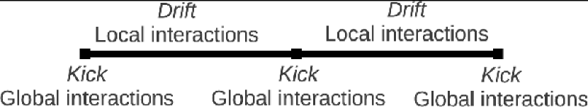
Figure 9: Schematic kick-drift-kick procedure for the generalized mixed-variable symplectic method [32].

4.4 Performance

The performance of the AMUSE framework depends on the codes used, the problem size, the choice of initial conditions and the interactions among the component parts as defined in the user script. It is therefore not possible to present a general account of the overhead of the framework, or the timing of the individual modules used. However, in order to provide some understanding of the time spent in the framework, as opposed to the community modules, we present the results of two independent performance analysis, one using a suite of 9 gravitational N-body solvers (Figs. 10 and 11) on three of which we report in more detail in Fig. 12, and analysis of a coupled hydrodynamics and gravitational dynamics solver in several framework solutions (Tab. 1).

4.4.1 Mono-physics solver performance

In Fig. 10 we compare the performance of several N-body solvers in AMUSE. Some of these solvers are GPU accelerated (ph4 and Bonsai [33]), others run on multiple cores (Fi [34, 35]), but most were run on a single processor even though they could have been run in parallel. Each calculation was run using standard parameters (double precision, time step of $dt=2^{-6}$ or an adaptive time step determined by the community code, an opening angle of $\theta=75^{\circ}$ for tree-codes, and $N^{-1/3}$ softening length). The initial conditions were selected from a Plummer [28] sphere in N-body units in which all particles had the same mass. The runs were performed for 10 N-body time units [36] and include framework overhead and analysis of the data, but not the generation of the initial conditions or spawning the community code.

For small $N$ ($\,{\raise-2.15277pt\hbox{$\buildrel<\over{\sim}$}}\ 10$) the performance of all codes saturates, mainly due to the start-up cost of the AMUSE framework, the construction of a tree for only a few particles, or communication with the GPU (which is particularly notable for Bonsai). For large $N$, the performance of the direct N-body codes (dashed curves) scales $\propto N^{2}$. The wall-clock time of the tree codes (solid curves) scale $\propto N\log N$, as expected, but with a rather wide range in start-up time for small N depending on the particulars of the implementation. The largest offset is measured for Bonsai; because of its relatively large start-up time of 0.2 s, its timing remains roughly constant until $N\simeq 10^{3}$, after which it performs considerably better than the other (tree)codes, which have a smaller offset but reach their terminal speed at relatively small $N$. It is in particular due to the use of the GPU that the start-up times for Bonsai (and also Octgrav, not shown) dominate until quite large $N$, and terminal speed is not reached until $N\,{\raise-2.15277pt\hbox{$\buildrel>\over{\sim}$}}\ 10^{4}$. These codes require large $N$ to fully benefit from the massive parallelism of the GPU.

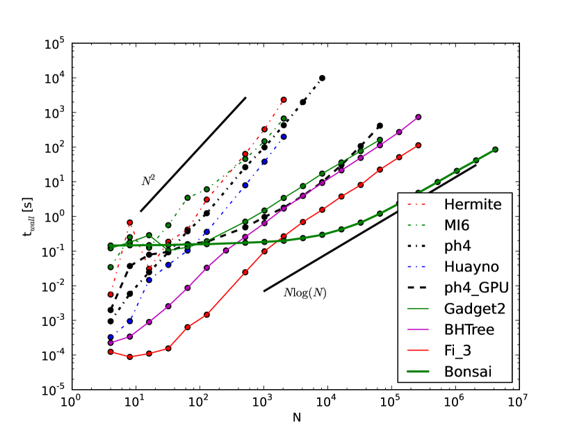
Figure 10: Wall clock time for 1 N-body time unit (averaged from running for 10 N-body time units) of a selection of 9 gravitational N-body solvers in the AMUSE framework. The direct codes are represented as dashed curves, the tree codes as solid lines. The scaling for direct N-body ($\propto N^{2}$) and tree algorithm ($\propto N\log N$) are indicated with the black solid lines. The 9 production quality codes include direct ($N^{2}$) N-body solvers with a $6^{th}$ order Hermite predictor corrector integrator (MI6 [37, 38]), several $4^{th}$ order Hermite integrators (Hermite [39], Ph4) semi-symplectic code based on Hamiltonian splitting integrator (Huayno), and a suite of tree codes (BHTree [31], Gadget2 [40], Bonsai [33]). For ph4 we also show the GPU accelerated version, which is realized using the Sapporo library. The performance of PhiGPU [41] is not shown because it is almost identical to that of ph4 with GPU support. The reasons for the similar performance stems from the use of the Sapporo GPU library for N-body solver, which are used by both codes. Also Octgrav [42] is omitted, which up to about $N\sim 10^{4}$ performs like Bonsai and then follows Fi. All runs ware carried out on a 4-core workstation with a Intel Xeon CPU E5620 operating at 2.40GHz and NVIDIA G96 (Quadro FX580) running generic 64-bit Ubuntu Linux kernel 2.6.35-32.

In Fig. 11 we present the fraction of the wall clock time (in Fig. 10) spent in the AMUSE framework. This figure gives a different perspective from Fig. 10. The tree codes perform generally worse in terms of efficiency, mainly because of the relatively small amount of calculation time spent in the N-body engine compared to the much more expensive direct N-body codes; this is particularly notable in Fi and Bonsai. Eventually, each code reaches a terminal efficiency, the value of which depends on the details of the implementation. Direct N-body codes tend to converge to an average overhead of $\,{\raise-2.15277pt\hbox{$\buildrel<\over{\sim}$}}\ 0.1$% of the runtime, whereas tree codes reach something like $\sim 1$% for the fastest code (Bonsai). The particular shape of the various curves depends on the scaling with $N$ of the work done by the community code and the framework. We can draw a distinction between generating the initial conditions ($\mathcal{O}(N)$), starting up the community module ($<\mathcal{O}(N)$), committing the particle data to the code ($\mathcal{O}(N)$), analyzing the data, and the actual work done in the community code. The scaling with $N$ of these last two tasks depends on the implementation — $\mathcal{O}(N^{2})$ for the direct codes and $\mathcal{O}(N\log N)$ for the tree codes.

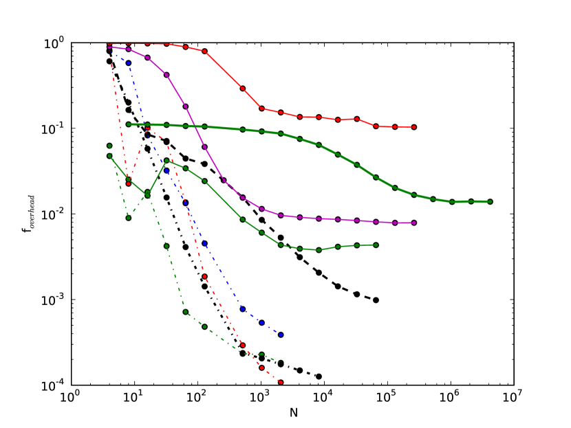
Figure 11: Overhead (fraction of time spent in the AMUSE framework) in a number of N-body simulation codes embedded in the AMUSE framework. The line styles are as in Fig. 10.

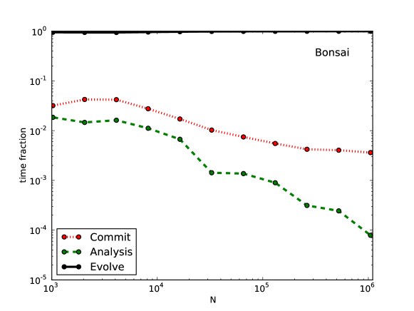
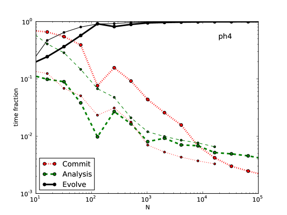
Figure 12: Fractional time spent in various parts of the framework as a function of the number of particles, $N$ for the Bonsai tree code (top panel) and for ph4 with and without GPU support using the Sapporo library (bottom panel, thick line with GPU, thin line without GPU). The top black curve gives time spent to integrate the equations of motion for a Plummer sphere with equal mass particles without softening for 1 N-body time unit. The lower curves, indicated in the legend detail the time for AMUSE to convert units and send the data to the spawned community code (commit) and the time spent in analyzing the data (analysis, which in this case also includes calculating the total kinetic and potential energy of the system).

In Fig. 12 we present a break down of the wall-clock times for three quite different community codes, but otherwise identical AMUSE scripts: the Barnes-Hut tree code Bonsai, and the direct code ph4 with and without GPU support. We separated the costs for running the community code, committing data to the code, and data analysis; the last two we call the framework overhead. Note that, in practice, the computationally intensive parts of the analysis calculations are performed by the modules, and not by the python framework. Therefore, the measurements of the framework overhead presented in Fig. 12 should be considered as upper limits. We ignored the cost for start-up (spawning the community code) and generating the initial conditions, because these are generally performed only once per run, even though they may have a time complexity similar to the underlying community code. For short runs with few particles these costs may be substantial, but for production simulations they result in negligible overhead.

The tree code (top panel in Fig. 12) has $N\log N$ time complexity (see Fig. 10) whereas analysis has an $N$ dependency. For small $N$ the framework cost may be quite substantial, but for larger simulations these costs become negligible ($<1$%). In the limit of large $N$, committing the particles has a time complexity similar to a tree code, but with a much smaller coefficient. For Bonsai, committing the particles limits the efficiency of the community code to about 99.6%. The direct N-body code (bottom panel in Fig. 12) has $N^{2}$ time complexity (see Fig. 10) and running large $N$ in the framework is even more favorable in terms of efficiency than running a tree code. The analysis and commit parts still have the same scaling with $N$, and for large $N$ less than 1% of the wall-clock time is spent in the framework. The difference between the GPU and CPU versions of the direct code is most evident in committing the data to the code, which is relatively slow for the GPU enabled code, and particularly severe for small $N$.

4.4.2 Multi-physics performance

One of the main advantages of AMUSE is the possibility of running different codes concurrently, with interactions among them, as discussed in §4.3.1. To explore the additional overhead generated in such cases, we present in Tab. 1 timings for a series of simulations combining gravitational dynamics and hydrodynamics. The timings listed in the table are determined using three different codes: the treeSPH code Fi [34, 35], the direct gravitational N-body code PhiGPU [41], and an analytic static background potential (identified as “field” in the top row of the table). The treeSPH code is implemented in FORTRAN90, the direct gravitational $N$-body code is in FORTRAN77, and the analytic tidal field is implemented in python.

The simulations were performed for N stars, each of one solar mass, in a cluster with a Plummer [28] initial density profile and a characteristic radius of 1 pc. We simulated the orbits of cluster stars within a cloud of gas having 9 times as much mass as in stars, and the same initial density distribution. The gas content was simulated using 10 $N$ gas particles. To treat the direct gravitational N-body solver PhiGPU in the same way as the tree-code Fi for solving the inter-particle gravity, we adopted a softening length of 0.01 pc for the stars. When employing Fi as an SPH code we adopted a smoothing length of 0.05 pc for the gas particles. The N-body time step was 0.01 N-body time units [36], and the interactions between the stellar- and fluid-dynamical codes were resolved using a Bridge time step of 0.125 N-body time units (see § 4.3.1, but for more details about the simulation see [26]).

The first column in Tab. 1 gives the number of stars in the simulation. Subsequent columns give the fraction of the wall-clock time spent in the AMUSE framework relative to the time spend in the two production codes. In the second column, we used Fi for the stars as well as for the gas particles. No Bridge was used in this case; rather, the stars were implemented as “massive dark particles” in the SPH code. For the simulations presented in the third column we used Bridge to couple the massive dark particles and the SPH particles, but both the gas dynamics and the gravitational stellar dynamics were again calculated using Fi as a gravitational tree-code. Not surprisingly, the AMUSE overhead using Bridge is larger than when all calculations are performed entirely within Fi (compare the second and third columns in Tab. 1), but for $N\,{\raise-2.15277pt\hbox{$\buildrel>\over{\sim}$}}\ 500$, the overhead in AMUSE becomes negligible. For $N=1000$ the simulation lasted 769.1 s  when using only Fi, whereas when we adopted Bridge the wall-clock time was 897.7 s. In production simulations the number of particles will generally greatly exceed 1000, and we consider the additional cost associated with the flexibility of using Bridge time well spent.

N	Fi	Fi+Fi	PhiGPU+Fi	Fi+field	PhiGPU+field
10	0.1980	0.563	0.243	0.943	0.170
50		0.129	0.109	0.885	0.308
100	0.0010	0.061	0.057	0.701	0.322
500		0.021	0.021	0.200	0.377
1000	0.0003	0.017	0.017	0.113	0.415
5000	0.0003	0.016	0.017	0.053	0.446

Table 1: Relative timing measurements of AMUSE in various configurations. The first column gives the number of star particles used in the simulations. Subsequent columns give the fraction of time spent in the AMUSE interface, rather than in the module(s). The relative timings in the second columns are performed using Fi as a stand alone module for both the gravity and the SPH inside AMUSE. For the other simulations we adopted a Bridge (see § 4.3.1) interface using two codes, for which we adopted Fi, PhiGPU, and a simple analytic tidal potential (field).

For small $N$ ($\,{\raise-2.15277pt\hbox{$\buildrel<\over{\sim}$}}\ 50$), a considerable fraction (up to 83%) of the wall-clock time is spent in the AMUSE framework. This fraction is high, particularly for the combination of PhiGPU and the analytic field, because of the small wall-clock time (less than 10 seconds) of these simulations. The complexity of both codes, $\mathcal{O}(N^{2})$ for PhiGPU and $\mathcal{O}(N)$ for the analytic external field introduces a relatively large overhead in the python layer compared to the gravity solver, in particular since the gravitational interactions are calculated using a graphical processing unit, which for a relatively small number of particles introduces a rather severe communication bottleneck. This combination of unfavorable circumstances cause even the $N=5000$ runs with PhiGPU and the tidal field to spend more than 50% of the total wall-clock time in the AMUSE framework. However, we do not consider this a serious drawback, since such calculations are generally only performed for test purposes. In this case it demonstrates that AMUSE has a range of parameters within which it is efficient, but that there is also a regime for which AMUSE does not provide optimal performance.

5 Discussion

We have described MUSE, a general software framework incorporating a broad palette of domain-specific solvers, within which scientists can perform detailed simulations combining different component solvers, within which scientists can perform detailed simulations using different component solvers, and AMUSE, an astrophysical implementation of the concept. The design goal of the environment is that it be easy to learn and use, and enable combinations and comparisons of different numerical solvers without the need to make major changes in the underlying codes.

One of the hardest, and only partly solved, problems in (A)MUSE is a general way to convert data structures from one type to another. In some cases such conversion can be realized by simply changing the units, or reorganizing a grid, but in more complex cases, for example, converting particle distributions to a tessellated grid, and vice versa, the solution is less clear. Standard procedures exist for some such conversions, but it is generally not guaranteed that the solution in unique.

Some drawbacks of realizing the inter-community module communication using MPI are the relatively slow response of spawning processes, the limited flexibility of the communication interface, and the replication of large data sets in multiple realizations of the same community module. Although it is straightforward to spawn multiple instances of the same code, these processes do not (by design) share data storage, aside from the data repository in the manager. For codes that require large data storage, for example look-up tables for opacities or other common physical constants, the data are reproduced as many times as the process is spawned. This limitation may be overcome by the use of shared data structures on multi-core machines, or by allowing inter-community module communication via “tunneling,” where data moves directly between community modules, rather than being channeled through the manager.

The python programming environment is not known for speed, although this is generally not a problem in AMUSE, since little time is spent in the user script and the underlying codes are highly optimized, allowing good overall performance. Typical monolithic software environments lose performance by unnecessary calls among domains; in MUSE this is prevented by the loose coupling between community modules. We have experimented with a range of possible ways to couple the various community modules, and can roughly quantify the degree to which community modules are coupled.

MUSE, as described here, is best suited for problems in which the different physical solvers are relatively weakly coupled. Weak and strong coupling may be distinguished by the ratio of the time intervals on which different community modules are called (see also §4). For time step ratios $\,{\raise-2.15277pt\hbox{$\buildrel<\over{\sim}$}}\ 1/10$, the AMUSE implementation gives excellent performance, but if the ratio approaches unity the MUSE approach becomes progressively more expensive. It is, however, not clear to what extent a monolithic solver will give better performance in these strongly coupled cases. The upshot is that there is a range of problems for which our implementation works well, but there are surely other interesting multi-physics problems in astrophysics and elsewhere for which this separation in scales is not optimal. However, we have experimented with more strongly coupled community modules, and have not yet found it to be a limiting factor in the system design.

References

- [1] P. P. Eggleton, MNRAS 163, 279 (1973).
- [2] R. A. Gingold, J. J. Monaghan, MNRAS 181, 375 (1977).
- [3] S. J. Aarseth, in Multiple time scales, p. 377 - 418, pp. 377–418 (1985).
- [4] B. Fryxell, et al., ApJS 131, 273 (2000).
- [5] M. Pharr, R. Fernando, GPU Gems 2 (Programming Techniques for High-Performance Graphics and General-Purpose Computation). Addison Wesley (2005), ISBN 0-321-33559-7.
- [6] J. McCarthy, P. Abrahams, D. Edwards, S. Hart, M. I. Levin, LISP 1.5 Programmer’s Manual: Object - a synonym for atomic symbol, p. 105. MIT Press (1962).
- [7] B. Kent, W. Cunningham, in OOPSLA ’87 workshop on Specification and Design for Object-Oriented Programming (1987).
- [8] P. Teuben, in R. A. Shaw, H. E. Payne, J. J. E. Hayes (eds.), Astronomical Data Analysis Software and Systems IV, vol. 77 of Astronomical Society of the Pacific Conference Series, p. 398 (1995).
- [9] J. Barnes, P. Hut, P. Teuben, Astrophysics Source Code Library p. 10051 (2010).
- [10] S. F. Portegies Zwart, S. L. W. McMillan, P. Hut, J. Makino, MNRAS 321, 199 (2001).
- [11] P. Hut, S. McMillan, J. Makino, S. Portegies Zwart, Astrophysics Source Code Library p. 10076 (2010).
- [12] S. F. Portegies Zwart, F. Verbunt, A&A 309, 179 (1996).
- [13] P. Hut, et al., New Astronomy 8, 337 (2003).
- [14] A. Sills, et al., New Astronomy 8, 605 (2003).
- [15] M. B. Davies, et al., New Astronomy 12, 201 (2006).
- [16] S. Portegies Zwart, et al., New Astronomy 14, 369 (2009).
- [17] E. Lusk, N. Doss, A. Skjellum, Parallel Computing 22, 789 (1996).
- [18] J. Maassen, H. Bal, in the 16th international symposium on High Performance Distributed Computing. New York, NY, USA, pp. 1–10 (2007).
- [19] F. J. Seinstra, et al., ‘Jungle computing: Distributed supercomputing beyond clusters, grids, and clouds’ (2011).
- [20] H. E. Bal, et al., Computer 43(8), 54 (2010).
- [21] N. Drost, et al., ArXiv e-prints (2012).
- [22] S. Portegies Zwart, S. McMillan, I. Pelupessy, A. van Elteren, ArXiv e-prints (2011).
- [23] S. McMillan, S. Portegies Zwart, A. van Elteren, A. Whitehead, ArXiv e-prints (2011).
- [24] S. Portegies Zwart, E. P. J. van den Heuvel, J. van Leeuwen, G. Nelemans, ApJ 734, 55 (2011).
- [25] M. S. Fujii, S. Portegies Zwart, Science 334, 1380 (2011).
- [26] F. I. Pelupessy, S. Portegies Zwart, MNRAS 420, 1503 (2012).
- [27] E. E. Salpeter, ApJ 121, 161 (1955).
- [28] H. C. Plummer, MNRAS 71, 460 (1911).
- [29] M. Fujii, M. Iwasawa, Y. Funato, J. Makino, Publ. Astr. Soc. Japan 59, 1095 (2007).
- [30] T. E. Hull, W. H. Enright, B. M. Fellen, A. E. Sedgwick, SIAM Journal on Numerical Analysis 9(4), pp. 603 (1972).
- [31] J. Barnes, P. Hut, Nat 324, 446 (1986).
- [32] J. Wisdom, M. Holman, AJ 102, 1528 (1991).
- [33] J. Bédorf, E. Gaburov, S. Portegies Zwart, Journal of Computational Physics 231, 2825 (2012).
- [34] F. I. Pelupessy, P. P. van der Werf, V. Icke, A&A 422, 55 (2004).
- [35] F. I. Pelupessy, P. P. Papadopoulos, P. van der Werf, ApJ 645, 1024 (2006).
- [36] D. C. Heggie, R. D. Mathieu, LNP Vol. 267: The Use of Supercomputers in Stellar Dynamics in P. Hut, S. McMillan (eds.), Lecture Not. Phys 267, Springer-Verlag, Berlin (1986).
- [37] K. Nitadori, J. Makino, New Astronomy 13, 498 (2008).
- [38] M. Iwasawa, S. An, T. Matsubayashi, Y. Funato, J. Makino, ApJL 731, L9 (2011).
- [39] P. Hut, J. Makino, S. McMillan, ApJL 443, L93 (1995).
- [40] V. Springel, MNRAS 364, 1105 (2005).
- [41] S. Harfst, et al., New Astronomy 12, 357 (2007).
- [42] E. Gaburov, J. Bédorf, S. Portegies Zwart, Procedia Computer Science, volume 1, p. 1119-1127 1, 1119 (2010).