Multibreathers in Klein-Gordon chains with interactions beyond nearest neighbors

Abstract

We study the existence and stability of multibreathers in Klein-Gordon chains with interactions that are not restricted to nearest neighbors. We provide a general framework where such long range effects can be taken into consideration for arbitrarily varying (as a function of the node distance) linear couplings between arbitrary sets of neighbors in the chain. By examining special case examples such as three-site breathers with next-nearest-neighbors, we find crucial modifications to the nearest-neighbor picture of one-dimensional oscillators being excited either in- or anti-phase. Configurations with nontrivial phase profiles emerge from or collide with the ones with standard ($0$ or $\pi$) phase difference profiles, through supercritical or subcritical bifurcations respectively. Similar bifurcations emerge when examining four-site breathers with either next-nearest-neighbor or even interactions with the three-nearest one-dimensional neighbors. The latter setting can be thought of as a prototype for the two-dimensional building block, namely a square of lattice nodes, which is also examined. Our analytical predictions are found to be in very good agreement with numerical results.

I Introduction

The initial numerical inception of anharmonic modes consisting of a few excited sites in nonlinear lattices sietak ; pa90 , and their subsequent placement on a rigorous existence basis (under rather generically satisfied non-resonance conditions) in macaub has triggered a huge growth of interest in the theme of the so-called discrete breathers. These are exponentially localized in space, periodic in time states which have subsequently been theoretically/numerically predicted and experimentally verified to arise in a very diverse host of applications. These include (but are not limited to) DNA double-strand dynamics in biophysics peyrard , coupled waveguide arrays and photorefractive crystals in nonlinear optics photon ; moti3 ; review_opt , breathing oscillations in micromechanical cantilever arrays sievers , Bose-Einstein condensates in optical lattices in atomic physics morsch , and granular crystals sen08 . The interest in this theme has also been mirrored in a wide array of reviews on methods of identifying and analyzing such intrinsically localized modes flach1 ; macrev ; flach2 ; aubrev .

More recently, the stability of the discrete breather configurations, especially in the case of the excitation of multiple sites has been of particular interest. One approach to obtaining relevant results consists of the so-called Aubry band theory aubrev , used e.g. in ACSA03 ; CAR05 . This led to the conclusion that for soft nonlinear potentials multi-breathers with any subset of adjacent sites being excited in-phase are unstable, while ones with all adjacent sites in anti-phase can be stable in the vicinity of the so-called anti-continuum limit of uncoupled anharmonic oscillators. A complementary theory that yields insights on both the existence and the stability of multibreathers has been pioneered by MacKay and collaborators; see e.g., mackay1 ; mac1 ; macsep . This is the so-called effective Hamiltonian method which is identified by averaging over the period of the unperturbed solution and developing the proper action-angle variables. The extrema of the resulting effective Hamiltonian determine the relative phases of adjacent excited sites in the multi-site breather solution, while the relevant Hessian is intimately connected to the Floquet multipliers of the associated periodic orbit. Using this methodology, the work of KK09 retrieved as well as refined the results of ACSA03 for arbitrary phase relations between the excited oscillators of such multi-breather configurations. The equivalence between these two basic methods and their conclusions was recently established in IJBC . We should also note in passing that similar results have been acquired also in configurations where there are “holes” between the excited breather sites pelisak , through higher order perturbation theory generalizing the above conclusions to the cases with one-site holes. On the other hand, the existence and stability of single/multi-site breathers have been studied in diatomic FPU lattices. The work of yoshi was based on a discrete Sturm theorem which necessitated (for the separation of the space $n$ and time $t$ variables) a potential which was at least purely quartic. In the realm of lattices with longer than the nearest-neighbor interactions a variety of issues have been considered such as, e.g. in FeckanRothos10 , the existence and bifurcation of quasi periodic traveling waves in nonlocal lattices with polynomial type potentials.

In the present work, we consider the generalization of the above settings, which are principally concerned with the interaction between nearest neighbors, to the case with longer range neighbor interactions for Klein-Gordon chains. Upon revisiting the nearest neighbor case and presenting the effective Hamiltonian formalism (of MacKay and collaborators) there (section II) for existence and stability of multibreathers, in section III, we generalize this formalism to the case of an arbitrary number of neighbors (denoted by $r$) interacting with each other. By specializing to the case of nearest and next-nearest neighbor interactions (and three-site breathers) as our first case example of the application of the results in section IV, we already infer the fundamental modifications to the standard picture that ensue due to interactions beyond nearest neighbors. These include configurations that have non-standard relative phases between adjacent oscillators, a feature which is absent in the nearest-neighbor interaction case kouk12 and also symmetry breaking bifurcations that arise due to the “collision” of branches of solutions with such non-trivial phase relations, with more standard ones with relative phases of $0$ or $\pi$ between adjacent oscillators. The generic nature of these conclusions is confirmed by considering the case examples of four-site breathers with next-nearest-neighbor interactions in section V and such breathers with interaction ranges of $r=3$ in section VI. The latter setting is very close to genuinely two-dimensional setting in a square lattice plaquette, which constitutes our final example in section VII. We close our presentation by some remarks on the parallels of our results with the simpler case of the discrete nonlinear Schrödinger lattices pgkbook (section VIII), which has been examined earlier in pgkpla ; chong , as well as a summary of our conclusions and some future directions (section IX).

II Background: The Classical Klein-Gordon chain

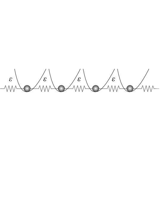
Figure 1: The classical nearest-neighbor Klein-Gordon chain

The Hamiltonian of a Klein-Gordon chain with nearest neighbor interactions is the following

$$H=H_{0}+\varepsilon H_{1}=\sum_{i=-\infty}^{\infty}\left[\frac{1}{2}p_{i}^{2}+V(x_{i})\right]+\frac{\varepsilon}{2}\sum_{i=-\infty}^{\infty}\left(x_{i}-x_{i-1}\right)^{2},$$ (1)

which leads to the equations of motion

$$\ddot{x_{i}}=-V^{\prime}(x_{i})+\varepsilon(x_{i-1}-2x_{i}+x_{i+1}).$$

It is well known that this system supports discrete breather, as well as, multibreather solutions. As indicated above, there are several papers dealing with the existence and stability of these motions; see e.g. macaub ; sepmac ; koukicht1 ; koukmac ; mackay1 ; ACSA03 ; KK09 ; pelisak .

II.1 Persistence of mutibreathers

In the anti-continuum limit $\varepsilon=0$, we consider all the oscillators of the chain at rest except for $n+1$ “central” ones which move in periodic orbits of frequency $\omega$. As indicated in pelisak , it is possible to generalize considerations to the case where not all of these oscillators are adjacent to each other, however, we will not concern ourselves with this additional complication herein. The time-periodic and space-localized motion of our excited oscillators will persist for $\varepsilon\neq 0$ to provide multibreathers of the same frequency $\omega$, if the phase difference between the succesive central oscillators satisfies specific conditions. In mackay1 it was shown that multibreathers correspond to critical points of $H^{\mathrm{eff}}$ which in first order of approximation is given by $H^{\mathrm{eff}}=H_{0}(I_{i})+\varepsilon\langle H_{1}\rangle(\phi_{i},I_{i})$ koukmac . The variables $\phi_{i}=w_{i+1}-w_{i}$ denote the $n$ phase differences of the $n+1$ successive central oscillators, while $I_{i}$ are given by $I_{i}=\sum_{j=i}^{n}J_{j}$, where $(J_{i},w_{i})$ are the action-angle variables of each uncoupled oscillator.

The average value of the coupling part of the Hamiltonian

$$\langle H_{1}\rangle(\phi_{i},I_{i})=\frac{1}{T}\oint H_{1}(w_{0},\phi_{i},I_{i}){\mathrm{d}}t$$

is calculated along the orbits in the anti-continuum limit $\varepsilon=0$.

This yields the conclusion that the persistence conditions for the existence of $n+1$-site multibreathers are

$$\frac{\partial\langle H_{1}\rangle}{\partial\phi_{i}}=0,\quad i=1\ldots n,$$ (2)

Note that the persistence conditions are the same for every lattice case where the Hamiltonian can be written in the for $H=H_{0}+\varepsilon H_{1}$ with $\frac{\partial\langle H_{1}\rangle}{\partial\phi_{i}}\not\equiv 0$. For a more detailed description of the above procedure one can also see KK09 .

The motion of the central oscillators for $\varepsilon=0$ can be described by

$$x_{i}(w_{i})=\sum_{m=0}^{\infty}A_{m}(J_{i})\cos(mw_{i}).$$ (3)

Since the action $J_{i}$ remains constant along an orbit in the anticontinuum limit, $x_{i}$ depends only on $w_{i}$. So, the average value of $H_{1}$ becomes (KK09 appendix A)

$$\langle H_{1}\rangle=-\frac{1}{2}\sum_{m=1}^{\infty}\sum_{s=1}^{n}A_{m}^{2}\cos(m\phi_{s})$$

and the persistence conditions (2) become in the case of Klein-Gordon chains with nearest neighbor interactions,

$$\frac{\partial\langle H_{1}\rangle}{\partial\phi_{i}}=0\Rightarrow M(\phi)\equiv\sum_{m=1}^{\infty}mA_{m}^{2}\sin(m\phi_{i})=0,\quad i=1\ldots n.$$ (4)

The function $M(\phi)$ possesses the obvious solutions $\phi_{i}=0,\pi$, while it has no others, as it is shown in kouk12 .

II.2 Stability of multibreathers

The spectral stability of the above mentioned multibreather solutions or, equivalently, the linear stability of the corresponding periodic orbits is determined through its characteristics exponents $\sigma_{i}$. These exponents are connected with the corresponding Floquet multipliers by the relation

$$\lambda_{i}=e^{\sigma_{i}T},$$

where $T=2\pi/\omega$ is the period of the multibreather. Due to the Hamiltonian character of the system there is a pair of exponents identically equal to zero. The non-zero characteristic exponents of the central oscillators correspond to the eigenvalues of the $(2n\times 2n)$ stability matrix mackay1 ${\bf E}={\bf\Omega}D^{2}H^{\mathrm{eff}}$, where $\Omega$ is the matrix of the symplectic form ${\bf\Omega}=\left(\begin{array}[]{cc}\bf O&-\bf I\\ \bf I&\bf O\end{array}\right)$ and $\bf I$ is the $n\times n$ identity matrix. The effective Hamiltonian $H^{\mathrm{eff}}$, as it has already been mentioned, in first order of approximation is given by $H^{\mathrm{eff}}=H_{0}+\varepsilon\langle H_{1}\rangle$. So, the stability matrix $\bf E$, to leading order of approximation and by taking into consideration the form of $H^{\mathrm{eff}}$, becomes

$$\bf E=\left(\begin{array}[]{c|c}\bf A&\bf B\\ \hline\cr\bf C&\bf D\end{array}\right)=\left(\begin{array}[]{c|c}\varepsilon\bf A_{1}&\varepsilon\bf B_{1}\\ \hline\cr\bf C_{0}+\varepsilon\bf C_{1}&\varepsilon\bf D_{1}\end{array}\right)=\left(\begin{array}[]{c|c}-\varepsilon\displaystyle\frac{\partial^{2}\langle H_{1}\rangle}{\partial\phi_{i}\partial I_{j}}&-\varepsilon\displaystyle\frac{\partial^{2}\langle H_{1}\rangle}{\partial\phi_{i}\partial\phi_{j}}\\[10.0pt] \hline\cr\\[-8.0pt] \displaystyle\frac{\partial^{2}H_{0}}{\partial I_{i}I_{j}}+\displaystyle\varepsilon\frac{\partial^{2}\langle H_{1}\rangle}{\partial I_{i}\partial I_{j}}&\displaystyle\varepsilon\frac{\partial^{2}\langle H_{1}\rangle}{\partial\phi_{j}\partial I_{i}}\end{array}\right).$$ (5)

Since the only possible solutions are the ones with $\phi_{i}=0,\pi$ and we consider central sites oscillating with the same frequency $\omega$, we get that $\bf A_{1}=D_{1}=0$ and so, the nonzero characteristic exponents are given to leading order of approximation by

$$\sigma_{\pm i}=\pm\sqrt{\varepsilon\,\chi_{1i}}+{\cal O}(\varepsilon^{3/2})\quad i=1\ldots n,$$ (6)

where $\chi_{1i}$ are the eigenvalues of the matrix $\bf B_{1}\cdot C_{0}$. Due to the form of the $J\mapsto I$ transformation the $\bf C_{0}$ matrix becomes (see KK09 appendix B)

$${\bf C_{0}}=\frac{\partial^{2}H_{0}}{\partial I_{i}\partial I_{j}}=-\frac{\partial\omega}{\partial J}\cdot{\bf L}=-\frac{\partial\omega}{\partial J}\cdot\left(\begin{array}[]{ccccc}2&-1&0&&\\ -1&2&-1&0&\\ &\ddots&\ddots&\ddots&\\ &0&-1&2&-1\\ &&0&-1&2\end{array}\right).$$

So, (6) becomes, up to leading order terms,

$$\sigma_{\pm i}=\pm\sqrt{\displaystyle-\varepsilon\frac{\partial\omega}{\partial J}{\chi_{z}}_{i}}\quad i=1\ldots n,$$ (7)

where ${\chi_{z}}_{i}$ are the eigenvalues of ${\bf Z}={\bf B_{1}\cdot L}$.

For systems of the form (1) we get

$${\bf B_{1}}=\displaystyle\frac{\partial^{2}\langle H_{1}\rangle}{\partial\phi_{i}\partial\phi_{j}}=\left\{\begin{array}[]{cl}f_{i}&\mathrm{for}\ i=j\\ 0&\mathrm{for}\ i\neq j\end{array}\right.,$$

with

$$f_{i}=f(\phi_{i})=\frac{1}{2}\sum_{m=1}^{\infty}m^{2}A_{m}^{2}\cos(m\phi_{i}).$$ (8)

So, $\bf Z$ can be written as

$${\bf Z}={\bf B_{1}}\cdot{\bf L}=\left(\begin{array}[]{ccccc}f_{1}&0&0&&\\ 0&f_{2}&0&0&\\ &\ddots&\ddots&\ddots&\\ &0&0&f_{n-1}&0\\ &&0&0&f_{n}\end{array}\right)\cdot\left(\begin{array}[]{ccccc}2&-1&0&&\\ -1&2&-1&0&\\ &\ddots&\ddots&\ddots&\\ &0&-1&2&-1\\ &&0&-1&2\end{array}\right)=\left(\begin{array}[]{ccccc}2f_{1}&-f_{1}&0&&\\ -f_{2}&2f_{2}&-f_{2}&0&\\ &\ddots&\ddots&\ddots&\\ &0&-f_{n-1}&2f_{n-1}&-f_{n-1}\\ &&0&-f_{n}&2f_{n}\end{array}\right)$$ (9)

Note that, for linear stability we require all the Floquet multipliers to lie on the unit circle, which is tantamount to all the characteristic exponents being purely imaginary. This depends on the sign of $P=\varepsilon\frac{\partial\omega}{\partial J}$ and the sign of $\chi_{z}$ as it can be seen from (7). Finally, by using some counting theorems KK09 for (9), we obtain:

Theorem 1.

KK09 In systems of the form (1), if $P\equiv\varepsilon\frac{\partial\omega}{\partial J}<0$ the only configuration which leads to linearly stable multibreathers, for $|\varepsilon|$ small enough, is the one with $\phi_{i}=\pi\quad\forall i=1\ldots n$ (anti-phase multibreather), while if $P>0$ the only linearly stable configuration, for $|\varepsilon|$ small enough, is the one with $\phi_{i}=0\quad\forall i=1\ldots n$ (in-phase multibreather). Moreover, for $P<0$ (respectively, $P>0$), for unstable configurations, their number of unstable eigenvalues will be precisely equal to the number of nearest neighbors which are in- (respectively, in anti-) phase between them.

Remark 1: Note that, the form of the matrix $\bf C_{0}$ is such due to the form of the $J\mapsto I$ transformation and the fact that in the anti-continuum limit $\frac{\partial H_{0}}{\partial J}=\omega$ and $\omega_{i}=\omega\ \mathrm{for}\ i=1\ldots n$. So, it is independent of the range of the interaction between the oscillators of the chain and it will remain the same in what follows. On the other hand, the diagonal form of $\bf B_{1}$ will change if longer range interactions are added to the system. So, the theorem will no longer hold but the general methodology will still apply and the characteristic exponents of the multibreather will be given by (7). We will consider this case in what follows.

Remark 2: In our previous works we used the term “out-of-phase” for $\phi=\pi$ configurations. This was because the only out-of-phase configuration was the $\phi=\pi$ one. In the present work, since, as we will see in the next section, there are out-of phase configurations with $\phi\neq\pi$, we use the term “anti-phase” for the $\phi=\pi$ configuration.

III Klein-Gordon chain with long range interactions

The picture radically changes when the chain involves interactions with range longer than mere nearest neighbors. The range parameter $r$ will be used to indicate the interaction length between the oscillators of the chain. So, for the classic nearest neighbor chain the range is $r=1$ as shown in fig. 1 while for the next nearest neighbor (NNN) chain the range is $r=2$ as illustrated in fig. 2 etc. The coupling force between the oscillators of the chain is linear and the coupling constants $\varepsilon_{i},i=1\ldots r$ are not, in general, equal.

The Hamiltonian of a 1D KG chain with long range interactions is:

$$H=\sum_{i=-\infty}^{\infty}[\frac{p_{i}^{2}}{2}+V(x_{i})]+\frac{1}{2}\sum_{i=-\infty}^{\infty}\sum_{j=1}^{r}\varepsilon_{j}\left(x_{i}-x_{i+j}\right)^{2}$$ (10)

which leads to the equations of motion

$$\ddot{x_{i}}=-V^{\prime}(x_{i})+\sum_{j=1}^{r}\varepsilon_{j}(x_{i-j}-2x_{i}+x_{i+j})$$

III.1 Persistence of multibreathers

Let $\varepsilon_{j}=k_{j}\varepsilon$, with $k_{1}=1$, then the Hamiltonian (10) becomes

$$H=H_{0}+\varepsilon H_{1}=\sum_{i=-\infty}^{\infty}[\frac{p_{i}^{2}}{2}+V(x_{i})]+\frac{\varepsilon}{2}\sum_{i=-\infty}^{\infty}\sum_{j=1}^{r}k_{j}\left(x_{i}-x_{i+j}\right)^{2}$$ (11)

Now, since the Hamiltonian is written in the form $H_{0}+\varepsilon\langle H_{1}\rangle$ the persistence conditions (2) can be used. If we consider again $n+1$ “central” oscillators and $x_{i}=\sum_{m=0}^{\infty}A_{m}\cos(mw_{i})$, we get for this case

$$\langle H_{1}\rangle=-\frac{1}{2}\sum_{m=1}^{\infty}\sum_{j=1}^{r}\sum_{s=1}^{n-j+1}A_{m}^{2}k_{j}\cos(m\sum_{l=0}^{j-1}\phi_{s+l}).$$ (12)

Note that, in the above we considered $r\leqslant n$ since any interaction of oscillators with $r>n$ does not affect the calculations, which are performed in the anti-continuum limit. So, if one considers $r>n$ then for the calculations in this section it would be equivalent to the choice of $r=n$. By differentiating Eq. 12 with respect to $\phi_{i}$ we get

$$\frac{\partial\langle H_{1}\rangle}{\partial\phi_{i}}=0\Rightarrow\sum_{m=1}^{\infty}\sum_{p=1}^{r}\sum_{s=z_{1}}^{z_{2}}mA_{m}^{2}k_{p}\sin(m\sum_{l=0}^{p-1}\phi_{s+l})=0,$$ (13)

or, by taking into consideration the definition of (4),

$$\sum_{p=1}^{r}\sum_{s=z_{1}}^{z_{2}}k_{p}M(\sum_{l=0}^{p-1}\phi_{s+l})=0,$$ (14)

where $z_{1}=\mathrm{max}(1,i-p+1)$ and $\displaystyle z_{2}=\left\{\begin{array}[]{ccc}i&\mathrm{for}&i+p-1\leqslant n\\ n-p+1&\mathrm{for}&i+p-1>n\end{array}\right.$.

Eqs. 12 and 13 (or 14) may be seem cumbersome to handle, they are much easier to use in the concrete examples that will follow in the next sections.

III.2 Stability of multibreathers

As we have already mentioned the characteristic exponents of the multibreather provided by the persistence conditions (13) are given, to leading order of approximation, by (7), i.e.

$$\sigma_{\pm i}=\pm\sqrt{\displaystyle-\varepsilon\frac{\partial\omega}{\partial J}{\chi_{z}}_{i}},\quad i=1\ldots n,$$

where ${\chi_{z}}_{i}$ are the eigenvalues of ${\bf Z}$ with

$${\bf Z}={\bf B_{1}\cdot L}=\frac{\partial^{2}\langle H_{1}\rangle}{\partial\phi_{i}\partial\phi_{j}}\cdot\left(\begin{array}[]{ccccc}2&-1&0&&\\ -1&2&-1&0&\\ &\ddots&\ddots&\ddots&\\ &0&-1&2&-1\\ &&0&-1&2\end{array}\right),\quad i,j=1\ldots n.$$ (15)

For linear stability we need all the characteristic exponents to be purely imaginary. So, if $P=\varepsilon\frac{\partial\omega}{\partial J}<0$ we need all the eigenvalues of $\bf Z$ to be negative, while if $P=\varepsilon\frac{\partial\omega}{\partial J}>0$ we need all the eigenvalues of $\bf Z$ to be positive.

Without loss of generality we can consider $i\leqslant j$, since the ${\bf B_{1}}$ matrix is symmetric. Let $d=j-i+1$, then the general form of $\frac{\partial^{2}\langle H_{1}\rangle}{\partial\phi_{i}\partial\phi_{j}}$ is

$$\frac{\partial^{2}\langle H_{1}\rangle}{\partial\phi_{i}\partial\phi_{j}}=\left\{\begin{array}[]{cl}0&\quad\mathrm{if}\quad d>r\\[8.0pt] \displaystyle\frac{1}{2}\sum_{m=1}^{\infty}\sum_{p=d}^{r}\sum_{s=z_{1}}^{z_{2}}m^{2}A_{m}^{2}k_{p}\cos(m\sum_{l=0}^{p-1}\phi_{s+l})&\quad\mathrm{if}\quad d\leqslant r\end{array}\right.,$$ (16)

or, by taking under consideration the definition of (8),

$$\frac{\partial^{2}\langle H_{1}\rangle}{\partial\phi_{i}\partial\phi_{j}}=\left\{\begin{array}[]{cl}0&\quad\mathrm{if}\quad d>r\\[8.0pt] \displaystyle\sum_{p=d}^{r}\sum_{s=z_{1}}^{z_{2}}k_{p}f(\sum_{l=0}^{p-1}\phi_{s+l})&\quad\mathrm{if}\quad d\leqslant r\end{array}\right..$$ (17)

Now $z_{1}$ is given by $z_{1}=\mathrm{max}(1,i-p+d)$, while $z_{2}$ is still given by $\displaystyle z_{2}=\left\{\begin{array}[]{ccc}i&\mathrm{for}&i+p-1\leqslant n\\ n-p+1&\mathrm{for}&i+p-1>n\end{array}\right..$

In order to demonstrate the use of the results of this section, in what follows, we will examine some particular cases.

IV 3-site breathers with $r=2$

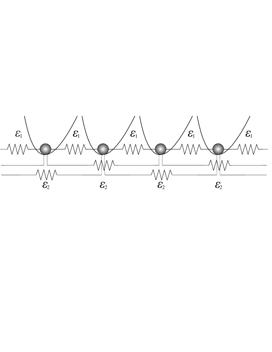
Figure 2: The $r=2$ Klein-Gordon chain with next nearest neighbor interactions

IV.1 The $\varepsilon_{1}=\varepsilon_{2}=\varepsilon$ case

IV.1.1 Persistence of multibreathers

The simplest case to check the effect of long range interactions is the one of 3 central oscilators (i.e. $n=2$) and range $r=2$. As we have already mentioned, any range $r>2$ would not affect our calculations. First we will check the case $k_{1}=k_{2}=1\Rightarrow\varepsilon_{1}=\varepsilon_{2}=\varepsilon$.

In this case the Hamiltonian (11) reads

$$H=H_{0}+\varepsilon H_{1}=\sum_{i=-\infty}^{\infty}\frac{1}{2}p_{i}^{2}+V(x_{i})+\frac{\varepsilon}{2}\sum_{i=-\infty}^{\infty}\left[(x_{i}-x_{i+1})^{2}+(x_{i}-x_{i+2})^{2}\right].$$

Since we consider a 3-site breather, $H_{1}$ becomes at the anti-continuum limit

$$H_{1}=x_{1}^{2}+x_{2}^{2}+x_{3}^{2}+(x_{1}-x_{2})^{2}+(x_{1}-x_{3})^{2}+(x_{2}-x_{3})^{2}$$

and

$$\langle H_{1}\rangle=-\frac{1}{2}\sum_{m=1}^{\infty}A_{m}^{2}\left\{\cos(m\phi_{1})+\cos(m\phi_{2})+\cos[m(\phi_{1}+\phi_{2})]\right\},$$

according also to (12), for $n=2$ and $r=2$. The persistence conditions (13) become

$$\frac{\partial\langle H_{1}\rangle}{\partial\phi_{i}}=0\Rightarrow\sum_{m=1}^{\infty}mA_{m}^{2}\left\{\sin(m\phi_{i})+\sin[m(\phi_{1}+\phi_{2})]\right\}=0,\quad\text{for}\quad i=1,2$$ (18)

or, by taking into consideration the definition of $M(\phi)$ in (4),

$$M(\phi_{i})+M(\phi_{1}+\phi_{2})=0,\quad\text{for}\quad i=1,2.$$ (19)

This equation, in addition to the standard solutions

$$\phi_{i}=0,\pi,$$

provides also the solutions

$$\phi_{1}=\phi_{2}=2\pi/3,\phi_{1}=\phi_{2}=4\pi/3.$$

The multibreather solutions with $\phi_{i}\neq 0$ are called phase-shift multibreathers or phase-shift breathers. The anti-phase and phase-shift configurations are depicted in figs. 3 and 4. For a better visualization one can also refer to videos 1 and 3 in videolink (video2 shows an in-phase configuration).

In order to produce these figures (and videos) we used the on-site potential $V(x)=\displaystyle\frac{x^{2}}{2}-0.15\frac{x^{3}}{3}-0.05\frac{x^{4}}{4}$ and initial conditions which correspond to motion with period $T=7$ and frequency $\omega=2\pi/T=2\pi/7\simeq 0.8976$. The same potential is used for every numerical calculation throughout this work, although it is straightforward to apply the relevant notions to arbitrary potentials of the Klein-Gordon type.

Remark 1: The persistence conditions (19) provide 2 equations.

$$\begin{array}[]{l}M(\phi_{1})+M(\phi_{1}+\phi_{2})=0\\ M(\phi_{2})+M(\phi_{1}+\phi_{2})=0.\end{array}$$ (20)

By substraction of equations (20) we get

$$M(\phi_{1})=M(\phi_{2})$$ (21)

which has, besides the trivial solutions $\phi_{i}=0,\pi$, two other obvious solutions: $\phi_{1}=\phi_{2}$ and $\phi_{1}+\phi_{2}=\pi$ for $0\leqslant\phi_{i}\leqslant 2\pi$. The last solution does not provide any new information because by substituting this into equations (20) we get $M(\phi_{1})=M(\phi_{2})=0$, which , as it is shown in kouk12 , only possesses the $\phi_{i}=0,\pi$ solutions. But the $\phi_{1}=\phi_{2}=\phi$ solution can reduce the two equations (20) into equation (22)

$$M(\phi)+M(2\phi)=0.$$ (22)

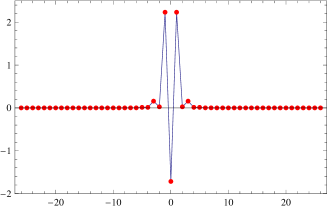
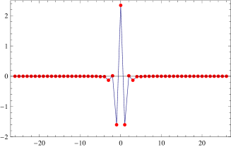
Figure 3: Two snapshots of a 3-site ($n=2$), anti-phase ($\phi_{1}=\phi_{2}=\pi$) multibreather in a range $r=2$ Klein-Gordon chain with $\varepsilon_{1}=\varepsilon_{2}=0.02$ and frequency $\omega=2\pi/7$. See also video1 in videolink .

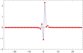
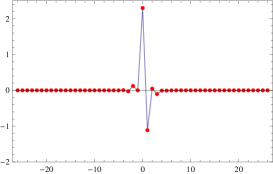
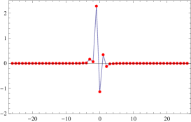
Figure 4: Three snapshots of a 3-site ($n=2$), phase-shift ($\phi_{1}=\phi_{2}\neq 0,\pi$) multibreather in a range $r=2$ Klein-Gordon chain with $\varepsilon_{1}=\varepsilon_{2}=0.02$ and frequency $\omega=2\pi/7$. See also video3 in videolink .

Remark 2: Our numerical computations strongly suggest that for all the phase-shift solutions it is $\phi_{1}=\phi_{2}$, yet a rigorous proof of this fact is still an open problem. So, equation (22) can be used in order to calculate all the solutions of the persistence conditions (19), except for the mixed one {$\phi_{1}=0,\ \phi_{2}=\pi$} (or equivalently {$\phi_{1}=\pi,\ \phi_{2}=0$}).

Remark 3: In the case under consideration ($n=2$, $r=2$, $k_{i}=1$), all the available solutions correspond to $\phi_{i}$’s which make each of the terms of the sum vanish in (18) which obviously provides a zero total.

Remark 4: The case under consideration is equivalent to the $3$-site breathers on a hexagonal lattice which has already been studied in koukmac ; kouketal . It can be effectively considered as a one-dimensional realization of such a lattice. In that context, the phase-shift multibreathers can be alternatively thought as “discrete vortices”, as they are solutions which complete a phase rotation by $2\pi$, as one traverses a discrete contour (which consists of the relevant triangle of sites).

Remark 5: As an aside, it should be mentioned that an additional motivation for the consideration of such next-nearest neighbor interactions stems from the consideration of zigzag arrays, similar to the waveguide arrays proposed theoretically in the context of nonlinear optics (and hence in the realm of the DNLS equation) in efremdnc .

Remark 6: The stability of the above mentioned breathers will be discussed at the end of the next section as a special case of the more general unequal coupling one.

IV.2 The $\varepsilon_{1}\neq\varepsilon_{2}$ case

IV.2.1 Persistence of multibreathers

Although the $\varepsilon_{1}=\varepsilon_{2}$ case is the easiest and allows us to perform some analytic calculations as well, the natural consideration for the case of next-nearest neighbors is the one with $\varepsilon_{1}\neq\varepsilon_{2}$. Intuitive physical considerations suggest to enforce $\varepsilon_{1}\geqslant\varepsilon_{2}$ (considering coupling force decreasing with the distance between the oscillators) but there are configurations (like the zigzag one) which may also justify settings with $\varepsilon_{1}<\varepsilon_{2}$ efremdnc . Let $k_{1}=1$ and $k_{2}=k$ or, $\varepsilon_{1}=\varepsilon$ and $\varepsilon_{2}=k\varepsilon$. In this case, the Hamiltonian (11) reads

$$H=H_{0}+\varepsilon H_{1}=\sum_{i=-\infty}^{\infty}\frac{1}{2}p_{i}^{2}+V(x_{i})+\frac{\varepsilon}{2}\sum_{i=-\infty}^{\infty}\left[(x_{i}-x_{i-1})^{2}+k(x_{i}-x_{i-2})^{2}\right].$$

Since we consider a $3$-site breather ($n=2$) we have only two independent $\phi_{i}$’s in the anti-continuum limit and by (12) we get

$$\langle H_{1}\rangle=-\frac{1}{2}\sum_{m=1}^{\infty}A_{m}^{2}\left\{\cos(m\phi_{1})+\cos(m\phi_{2})+k\cos[m(\phi_{1}+\phi_{2})]\right\}.$$

This leads to the persistence conditions:

$$\frac{\partial\langle H_{1}\rangle}{\partial\phi_{i}}=0\Rightarrow\sum_{m=1}^{\infty}mA_{m}^{2}\left\{\sin(m\phi_{i})+k\sin[m(\phi_{1}+\phi_{2})]\right\}=0\equiv M(\phi_{i})+kM(\phi_{1}+\phi_{2})=0\quad\text{for}\quad i=1,2.$$ (23)

Remark: By using the same arguments as in the previous section, if we consider $\phi_{1}=\phi_{2}$, we get from (23),

$$\sum_{m=1}^{\infty}mA_{m}^{2}\left[\sin(m\phi)+k\sin(2m\phi)\right]=0\equiv M(\phi)+kM(2\phi)=0.$$ (24)

So, one could use (24) instead of (23) as the relevant persistence condition in order to calculate all the solutions of (23) except of the mixed one {$\phi_{1}=0,\ \phi_{2}=\pi$} (or equivalently {$\phi_{1}=\pi,\ \phi_{2}=0$}).

In the $k=1$ ($\varepsilon_{1}=\varepsilon_{2}$) case, one could make a choice of $\phi_{1}=\phi_{2}=2\pi/3\ \mathrm{or}\ 4\pi/3$ in order to have $\left\{\sin(m\phi_{i})+\sin[m(\phi_{1}+\phi_{2})]\right\}=0$ $\forall m$, so that the total sum in (18) would vanish also. This is not possible in the $k\neq 1$ case. So, one may be led to believe that this is an isolated solution and that possibly there are no other solutions than $\phi=0$ and $\phi=\pi$ in this case. However, it instead turns out that there can be other solutions also which can be calculated numerically for $k\neq 1$. In fact, there is a critical value $k_{cr}=0.48286$ of $k$ where a pitchfork bifurcation occurs (fig. 5). For values $k<k_{cr}$ the only solutions Eq. (23) [or (24)] has are the trivial ones $\phi_{i}=0,\pi$. For $k>k_{cr}$, i.e., past the supercritical pitchfork bifurcation point, other solutions appear with $\phi_{i}\neq 0,\pi$ (phase-shift breathers) as is shown in fig. 5.

The bifurcation curve has been calculated in two ways. Firstly by numerically modeling the full system and secondly by numerically solving the transcendental existence conditions (23) using a small value of $\varepsilon=0.001$. The two curves practically coincide, which illustrates the remarkable accuracy of the theory in the vicinity of the anti-continuum limit.

A phase-shift breather with $k=0.54$ is depicted in fig. 7. For a better visualization of this breather one can also see video4 in videolink .

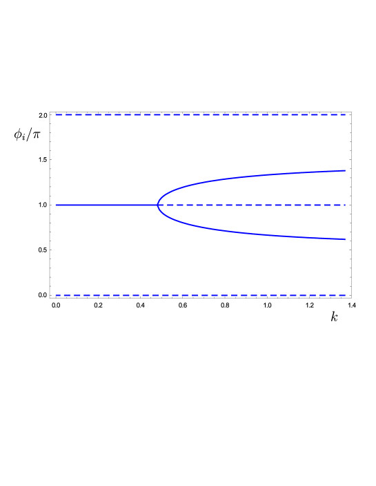
Figure 5: The bifurcation diagram for a 3-site ($n=2$) breather in a $r=2$ Klein-Gordon chain with $k=\varepsilon_{2}/\varepsilon_{1}$. A pitchfork bifurcation occurs for $k=k_{cr}=0.48286$. The curve is calculated using two methods. The first method is to use the full model, calculate the multibreather solutions with $\varepsilon=0.001$ and depict them as well as their stability. The second method is to solve numerically (23) and check when solutions with $\phi_{i}\neq 0,\pi$ appear. The curves produced with the two methods practically coincide (i.e., no difference is discernible at the scale of the plot). The various families that appear here are depicted in more detail in Fig. 6.

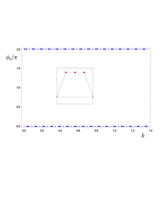
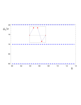
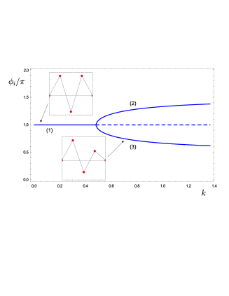
(a)	(b)	(c)

Figure 6: The various families that constitute Fig. 5 are depicted. Portraits of the configuration of the central oscillators for the different multibreather families are shown as insets in the corresponding diagrams. The line type in the figures depend in the number of positive ${\chi_{z}}$ (equivalently, the number of real eigenvalue pairs for $P\equiv\displaystyle\varepsilon\frac{\partial\omega}{\partial J}<0$) the corresponding family possesses: no positive ${\chi_{z}}$ corresponds to solid line, 1 positive ${\chi_{z}}$ corresponds to dashed line and 2 to dashed-dotted line. In (a) the in-phase configuration is depicted {$\phi_{1}=\phi_{2}=0\ (\text{or}\ 2\pi)$} which possesses 2 positive $\chi_{z}$. In (b) the mixed configuration is shown {$\phi_{1}=0,\ \phi_{2}=\pi$} which possesses 1 positive and 1 negative $\chi_{z}$. In (c) two families are shown. The first is the anti-phase one {$\phi_{1}=\phi_{2}=\pi$}. It has 2 negative $\chi_{z}$ until $k<k_{cr}=0.48286$ while it has 1 positive and 1 negative $\chi_{z}$ for $k>k_{cr}$. At this point the anti-phase family bifurcates to provide the phase-shift configuration {$\phi_{1}=\phi_{2}\neq 0,\pi$}. This family is represented by $\phi_{1}=\phi_{2}=(2)$ or $\phi_{1}=\phi_{2}=(3)$ and has no positive (2 negative) $\chi_{z}$. All of these together are depicted in Fig. 5. When two line segments coincide the more dense is shown.

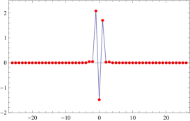
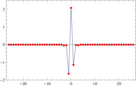
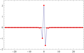
Figure 7: Snapshots of a phase-shift 3-site breather for $\varepsilon_{1}=0.02$ and $\varepsilon_{2}=k_{2}\varepsilon_{1}=0.56\varepsilon_{1}$ and frequency $\omega=2\pi/7$. See also video4 in videolink .

IV.2.2 Stability of multibreathers

By using the previously developed theory, we can calculate the characteristic exponents of the various configurations of 3-breathers in this lattice setting. The characteristic exponents of the specific solutions are given to first order of approximation by (7) as

$$\sigma_{\pm i}=\pm\sqrt{-\varepsilon\frac{\partial\omega}{\partial J}{\chi_{z}}_{i}},$$

where ${\chi_{z}}_{i}$ are the eigenvalues of the matrix ${\bf Z}$ defined in (15).

In the case under consideration of 3-site ($n=2$) breathers with range $r=2$ we have, also from (17),

$$\frac{\partial^{2}\langle H_{1}\rangle}{\partial\phi_{i}\partial\phi_{j}}=\left(\begin{array}[]{cc}f(\phi_{1})+kf(\phi_{1}+\phi_{2})&kf(\phi_{1}+\phi_{2})\\ kf(\phi_{1}+\phi_{2})&f(\phi_{2})+kf(\phi_{1}+\phi_{2})\end{array}\right)\quad\mathrm{and}\quad{\bf L}=\left(\begin{array}[]{cc}2&-1\\ -1&2\end{array}\right).$$

So, we get from (15),

$${\bf Z}=\frac{\partial^{2}\langle H_{1}\rangle}{\partial\phi_{i}\partial\phi_{j}}\cdot{\bf L}=\left(\begin{array}[]{cc}2f_{1}+kf_{1+2}&kf_{1+2}-f_{1}\\ kf_{1+2}-f_{2}&2f_{2}+kf_{1+2}\end{array}\right),$$

where the function $f(\phi)$ is defined as in (8), and $f_{1+2}\equiv f(\phi_{1}+\phi_{2})$, while $f_{i}=f(\phi_{i})$ for $i=1,2$ .

For linear stability it is required that all of the characteristic exponents be purely imaginary. So, the stability is determined by the sign of ${\chi_{z}}_{i}$.

In particular, we check the configurations that can appear in this case.

• $\phi_{1}=\phi_{2}$. This is the general case and includes the in-phase {$\phi_{1}=\phi_{2}=0$}, the out-of-phase {$\phi_{1}=\phi_{2}=\pi$} and phase-shift configurations {$\phi_{1}=\phi_{2}\neq 0,\pi$}. The corresponding eigenvalues $\chi_{z}$ are ${\chi_{z}}_{1}=3f_{\phi}$ and ${\chi_{z}}_{2}=f_{\phi}+2kf_{2\phi}$.
  

• $\phi_{1}=0,\phi_{2}=\pi$. This is the only solution with $\phi_{1}\neq\phi_{2}$. For this case it is ${\chi_{z}}_{1,2}=f_{0}+(1+k)f_{\pi}\pm\sqrt{f_{0}^{2}-(1+k)f_{0}f_{\pi}+f_{\pi}^{2}(1-k+k^{2})}$.
  

Remark: We have that $f_{0}>0$ as a direct consequence of the definition (8) of $f(\phi)$. On the other hand it is $f_{\pi}<0$. This can be rigorously proven (KK09 Lemma 3) but it can also be intuitively understood by the definition (8) of $f(\phi)$ and the fact that the first term of the Fourier expansion of $x(w)$ (3) is the dominant one. Using the same arguments we can conclude that $|f_{0}|>|f_{\pi}|$. So, we can immediately conclude that in the in-phase {$\phi_{1}=\phi_{2}=0$} configuration it is ${\chi_{z}}_{i}>0$, while in the mixed {$\phi_{1}=0,\ \phi_{2}=\pi$} configuration it is ${\chi_{z}}_{1}>0$, ${\chi_{z}}_{2}<0$.

On the other hand for the anti-phase {$\phi_{1}=\phi_{2}=\pi$} configuration, the formulas for the ${\chi_{z}}_{i}$ read

$${\chi_{z}}_{1}=3f_{\pi}\quad\text{and}\quad{\chi_{z}}_{2}=f_{\pi}+2kf_{0}.$$ (25)

The ${\chi_{z}}_{1}$ eigenvalue is always negative while the sign of the ${\chi_{z}}_{2}$ depends on the value of $k$. This can provide us with a criterion about the value of $k_{cr}$ where the bifurcation occurs, since, at this point ${\chi_{z}}_{2}$ changes sign. So, by (25) we get ${\chi_{z}}_{2}=0\Rightarrow k_{cr}=\displaystyle-\frac{f_{\pi}}{2f_{0}}$.

The values of $f_{0}$ and $f_{\pi}$ depend on the particular on-site potential as well as on the frequency we examine, so, the value $k_{cr}$ is not fixed. But, if we consider breathers with relatively low amplitude, which amounts to the breather frequency $\omega$ being close to the phonon frequency $\omega_{p}$, a rough estimation of $k_{cr}$ can be made. In such a case, the nonlinear character of the system is not fully revealed yet which means that the $A_{1}$ term in the development (3) is by far the most dominant one. This results to $|f_{0}|\simeq|f_{\pi}|$ and consequently $k_{cr}\simeq 0.5$.

In order to check our estimation, we perform some numerical calculations for the lattice with potential $V(x)=\displaystyle\frac{x^{2}}{2}-0.15\frac{x^{3}}{3}-0.05\frac{x^{4}}{4}$ which we use throughout this work, considering a motion with $\omega=2\pi/7\simeq 0.8976$. For this frequency, it is $\left|f_{0}/f_{\pi}\right|\simeq 1$, as can be seen in Fig. 8, so our estimation holds. In particular, it is $f_{\pi}=-1.48658$, $f_{0}=1.53934$ and $k_{cr}=\displaystyle-\frac{f_{\pi}}{2f_{0}}=0.48286$, which is precisely the value where the bifurcation occurs, while being very close also to the rough estimation (of $0.5$) above. Note that, as it can be seen in Fig. 8, if we had chosen a smaller breather frequency $\omega$, our estimation would be completely mistaken, since for small values of $\omega$ it is $\left|f_{0}/f_{\pi}\right|>1$.

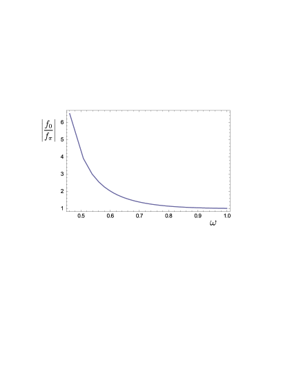
Figure 8: Dependence of the $\left|f_{0}/f_{\pi}\right|$ ratio with respect to the frequency $\omega$ of the breather.

Remarks about figs. 5 and  6: In figs. 5 and  6 all the multibreather families that exist in the present configuration ($n=2$, $r=2$) are shown. The multibreather families correspond to solution families of Eqs. 23. These families are categorized by the phase differences $\phi_{i}$ between the successive oscillators in the anticontinuous limit. The values of $\phi_{i}$ in the usual families ($\phi_{i}=0,\pi$) are constant with increasing $k$, while in the phase-shift ($\phi_{i}\neq 0,\pi$) families their values change with respect to $k$.

The various solution families are represented by various line (or curve) segments in the figures. The kind of the line depends on the number of positive ${\chi_{z}}$ (i.e., of real eigenvalue pairs for $P\equiv\displaystyle\varepsilon\frac{\partial\omega}{\partial J}<0$) that the corresponding solution has. So, for no $\chi_{z}>0$ we use a solid line, for one $\chi_{z}>0$ we use a dashed line while for two $\chi_{z}>0$ we use a dashed-dotted line. Since in Fig.  5 some of the families coincide, we separated the information in this figure into 3 panels in Fig. 6. These 3 panels together compose Fig. 5. If the segments which represent two or more distinct families of solutions coincide, the more dense is shown in the figure. In order to facilitate the visualization of the various families, we added insets in Figs. 6 demonstrating the profiles of (and hence illustrating the phase difference between) the central oscillators in the anticontinuum limit. This has as a result only solid and dashed segments to appear in Fig. 5. The families that are depicted in the figure are:

• {$\phi_{1}=\phi_{2}=0\ (\text{or}\ 2\pi)$} (in-phase). This family is shown in Fig. 6(a) and possesses 2 positive $\chi_{z}$.

• {$\phi_{1}=0\ \text{or}\ \pi,\ \phi_{2}=\pi$} (mixed). This family is depicted in Fig. 6(b) and possesses 1 positive and 1 negative $\chi_{z}$.

• {$\phi_{1}=\phi_{2}=\pi$} (anti-phase). It is represented in Fig. 6(c) by $\phi_{1}=\phi_{2}=(1)$. It has no positive $\chi_{z}$ until $k<k_{cr}$ while it has 1 positive and 1 negative $\chi_{z}$ for $k>k_{cr}$. At this point the $\phi_{1}=\phi_{2}=\pi$ family becomes subject to the bifurcation that gives rise to phase-shift multibreathers.

• $\phi_{1}=\phi_{2}\neq 0,\pi$ (phase-shift). This family is represented in Fig. 6(c) by $\phi_{1}=\phi_{2}=(2)$ or $\phi_{1}=\phi_{2}=(3)$ and has no positive $\chi_{z}$.

Since the stability of the multibreathers is also determined by the sign of $P\equiv\displaystyle\varepsilon\frac{\partial\omega}{\partial J}$, the above are summarized, in terms of stability of the solutions, in Table 1.

	$\hskip 14.22636ptP\hskip 14.22636pt$	$\hskip 19.91684ptk\hskip 19.91684pt$	In-phase $\phi_{1}=\phi_{2}=0$	Out-of-phase $\phi_{1}=\phi_{2}=\pi$	Phase-shift $\phi_{1}=\phi_{2}\neq 0,\pi$
Linear Stability	$P<0$	$k<k_{cr}$	unstable	stable	–
	$P<0$	$k>k_{cr}$	unstable	unstable	stable
	$P>0$	$k<k_{cr}$	stable	unstable	–
	$P>0$	$k>k_{cr}$	stable	unstable	unstable

Table 1: Stability of the various $n=2$, $r=2$, breather configurations depending on the values of $P\equiv\frac{\partial\omega}{\partial J}$ and $k$. With the dash we denote that this particular family does not exist for this range of values of $k$.

Stability of the various 3-site breather configurations in the $\varepsilon_{1}=\varepsilon_{2}$ case: Using the above derived results we can conclude what it is already known from koukmac ; kouketal . i.e. for $P<0$, as long as $k<k_{cr}$ the only stable configuration is the anti-phase one, while for $k>k_{cr}$ the stable configuration is the phase-shift one (which corresponds in this case to the “vortex” configuration of koukmac ; kouketal ). On the other hand for $P>0$ the only stable configuration is the in-phase one.

V 4-site breathers with $r=2$

In the next configuration we will consider four central oscillators, in order to study larger configurations, but we will keep the range to $r=2$ as a first step.

V.1 Persistence of multibreathers

We will treat the two cases $\varepsilon_{1}=\varepsilon_{2}$ and $\varepsilon_{1}\neq\varepsilon_{2}$ together, since the latter is a special case of the former with $k_{1}=k_{2}=1$. Since we consider 4 $(n=3)$ central oscillators and range $r=2$, (12) gives for $k_{1}=1$ and $k_{2}=k$,

$$\begin{array}[]{l}\displaystyle\langle H_{1}\rangle=-\frac{1}{2}\sum_{m=1}^{\infty}A_{m}^{2}\left\{\cos(m\phi_{1})+\cos(m\phi_{2})+\cos(m\phi_{3})+\right.\\ \left.\qquad\qquad\qquad\qquad+k\cos[m(\phi_{1}+\phi_{2})]+k\cos[m(\phi_{2}+\phi_{3})]\right\}\end{array}$$

while, the corresponding persistence conditions (13) become

$$\begin{array}[]{ccl}M(\phi_{1})+k\,M(\phi_{1}+\phi_{2})&=&0\\[8.0pt] M(\phi_{2})+k\left[M(\phi_{1}+\phi_{2})+M(\phi_{2}+\phi_{3})\right]&=&0\\[8.0pt] M(\phi_{3})+k\,M(\phi_{2}+\phi_{3})&=&0\end{array}$$

which have the trivial solutions $\phi_{i}=0,\pi$, as well as non trivial ones, as can be seen in fig. 9.

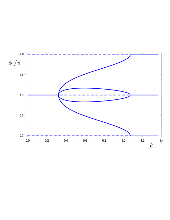
Figure 9: In this diagram all the existing families of 4-site ($n=3$) breathers in a KG chain with range $r=2$ are depicted. For a more detailed view of the particular families appearing in this diagram, refer also to fig. 10.

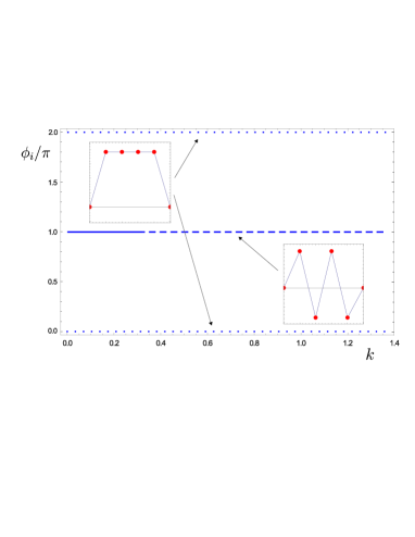
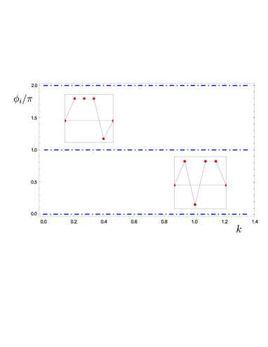
(a)		(b)
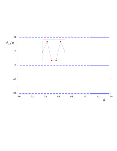
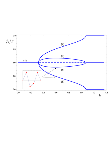
(c)		(d)

Figure 10: The various families that appear in Fig. 9 are depicted. Portraits of the configuration of the central oscillators for the different multibreather families are shown as insets in the corresponding diagrams. The line (or curve) type in the figures depends on the number of positive ${\chi_{z}}$ that the corresponding family possesses: no positive ${\chi_{z}}$ corresponds to a solid line, 1 positive ${\chi_{z}}$ corresponds to a dashed line, 2 to a dash-dotted and 3 to a dotted line. In (a) two multibreather families are depicted. The first is the in-phase one with {$\phi_{1}=\phi_{2}=\phi_{3}=0\ (\text{or}\ 2\pi)$} which possesses 3 positive $\chi_{z}$. The second one is the anti-phase one with {$\phi_{1}=\phi_{2}=\phi_{3}=\pi$}. It has no positive $\chi_{z}$ until $k<k_{cr}^{(1)}=0.3219$ while it has 1 positive $\chi_{z}$ for $k>k_{cr}^{(1)}$. At this point the anti-phase family gives rise, through a supercritical pitchfork, to the the phase-shift {$\phi_{1}=\phi_{2}\neq 0,\pi$} family. In (b) the mixed 1 configuration is shown {$\phi_{1}=\phi_{2}=0\ \text{or}\ 2\pi,\ \phi_{3}=\pi$} or {$\phi_{1}=\phi_{2}=\pi,\phi_{3}=0\ \text{or}\ 2\pi$}. These families possess 2 positive and 1 negative $\chi_{z}$ each. In (c) the mixed 2 family {$\phi_{1}=\phi_{3}=\pi,\phi_{2}=0\ \text{or}\ 2\pi$} is shown. It possesses 1 positive ${\chi_{z}}$ for $k<k_{cr}^{(2)}=1.0736$ and no positive ${\chi_{z}}$ for $k>k_{cr}^{(2)}$. At this point the mixed 2 family collides with the phase-shift one. In (d) the phase-shift {$\phi_{1}=\phi_{2}\neq 0,\pi$} family is shown and it is represented by $\phi_{1}=\phi_{3}=(3)$ and $\phi_{2}=(2)$ or $\phi_{1}=\phi_{3}=(4)$ and $\phi_{2}=(5)$. It exists for $k_{cr}^{(1)}<k<k_{cr}^{(2)}$. At $k=k_{cr}^{(1)}$ it bifurcates from the anti-phase family, while at $k=k_{cr}^{(2)}$ it emerges with the mixed 2 family, and possesses no positive $\chi_{z}$. Fig. 9 contains all of the above families together, where, when two line segments coincide the more dense is shown.

By using the same arguments as in the previous section, which are also verified by our numerical investigation we have that for all the phase-shift breathers it is $\phi_{1}=\phi_{3}$. At $k=k_{cr}^{(1)}=0.3219$ the anti-phase {$\phi_{1}=\phi_{2}=\phi_{3}=\pi$} family becomes subject to a bifurcation that generates the phase-shift 4-site breathers. We should also note in passing (see details below) that, in addition to this supercritical pitchfork, the figure reveals also a sub-critical pitchfork bifurcation that terminates the two asymmetric branches upon their collision with the branch with the mixed family {$\phi_{1}=\phi_{3}=\pi$, $\phi_{2}=0$} at $k_{cr}^{(2)}=1.0736$.

V.2 Stability of multibreathers

The stability of the existing multibreather solutions can be calculated by using the previously developed theory. Their corresponding characteristic exponents are given to first order of approximation by (7). In the case under consideration of 4-site ($n=3$) breathers with range $r=2$ we have from (16)

$$\frac{\partial^{2}\langle H_{1}\rangle}{\partial\phi_{i}\partial\phi_{j}}=\left(\begin{array}[]{ccc}f_{1}+k\,f_{1+2}&k\,f_{1+2}&0\\ k\,f_{1+2}&f_{2}+k\,f_{1+2}+k\,f_{2+3}&k\,f_{2+3}\\ 0&k\,f_{2+3}&f_{3}+k\,f_{2+3}\end{array}\right)\quad\mathrm{and}\quad{\bf L}=\left(\begin{array}[]{ccc}2&-1&0\\ -1&2&-1\\ 0&-1&2\end{array}\right)$$

So, (15) gives

$${\bf Z}=\frac{\partial^{2}\langle H_{1}\rangle}{\partial\phi_{i}\partial\phi_{j}}\cdot{\bf L}=\left(\begin{array}[]{ccc}2f_{1}+kf_{1+2}&kf_{1+2}-f_{1}&-kf_{1+2}\\ k(f_{1+2}-f_{2+3})-f_{2}&2f_{2}+k(f_{1+2}+f_{2+3})&k(f_{2+3}-f_{1+2})-f_{2}\\ -kf_{2+3}&kf_{2+3}-f_{3}&2f_{3}+kf_{2+3}\end{array}\right)$$

For the general case $\phi_{1}=\phi_{3}$, the eigenvalues of $\bf Z$ are

$${\chi_{z}}_{1}=2(f_{1}+kf_{1+2})\quad\text{and}\quad{\chi_{z}}_{2,3}=f_{1}+f_{2}+kf_{1+2}\pm\sqrt{f_{1}^{2}+f_{2}^{2}-2kf_{1}f_{1+2}+k^{2}f_{1+2}^{2}}.$$

The only configurations that are not included in the case above are the mixed ones {$\phi_{1}=\phi_{2}=0,\ \phi_{3}=\pi$} and {$\phi_{1}=\phi_{2}=\pi,\ \phi_{3}=0$}, which both have 2 positive $\chi_{z}$, independently of the value of $k$.

Remark: The ${\chi_{z}}_{2}$ eigenvalues of the anti-phase and mixed configurations can be used in order to calculate the values of $k_{cr}^{(1)}$ and $k_{cr}^{(2)}$. The ${\chi_{z}}_{2}$ for the anti-phase configuration is

$${\chi_{z}}_{2}=2f_{\pi}+kf_{0}+\sqrt{2f_{\pi}^{2}-2kf_{\pi}f_{0}+k^{2}f_{0}^{2}}.$$

Since for $k=k_{cr}^{(1)}$ it is ${\chi_{z}}_{2}=0$ we get $\displaystyle k_{cr}^{(1)}=-\frac{f_{\pi}}{3f_{0}}\simeq\frac{1}{3}$. The last rough estimation can be performed only when we consider breathers with frequency $\omega$ close to the phonon frequency $\omega_{p}$ (see also the discussion in the previous section), where $|f_{0}|\simeq|f_{\pi}|$. In order to be more precise, for the potential and frequency used in the present work, we get $k_{cr}=0.3219$.

On the other hand, the ${\chi_{z}}_{2}$ eigenvalue for the mixed {$\phi_{1}=\phi_{3}=\pi,\ \phi_{2}=0$} configuration is

$${\chi_{z}}_{2}=f_{0}+(1+k)f_{\pi}+\sqrt{(1-k)^{2}f_{\pi}^{2}+f_{0}}.$$

Since for $k=k_{cr}^{(2)}$ it is ${\chi_{z}}_{2}=0$ we get $k_{cr}^{(2)}=\displaystyle-\frac{f_{0}}{2f\pi+f_{0}}\simeq 1$ or, for the specific potential and frequency used in this work $k_{cr}^{(2)}=1.0736$.

Remarks on the stability diagram of Figs. 9 and 10: In Figs. 9 and 10 all the multibreather families they exist in the present configuration ($n=3$, $r=2$) are shown. The kind of the line (or curve) used for every segment depends on the number of positive ${\chi_{z}}$ as follows: no positive ${\chi_{z}}\rightarrow$ solid, 1 positive ${\chi_{z}}\rightarrow$ dashed, 2 positive ${\chi_{z}}\rightarrow$ dashed-dotted, 3 positive ${\chi_{z}}\rightarrow$ dotted. All the families shown in Fig.10 are depicted together in Fig.9. Since, if two segments coincide, the more dense is shown, in Fig.9 we can see only solid and dashed segments. The families which are depicted in these two figures are the following:

• {$\phi_{1}=\phi_{2}=\phi_{3}=0\ (\text{or}\ 2\pi)$} (in-phase). This family is shown in Fig.10(a) and has 3 positive $\chi_{z}$.

• {$\phi_{1}=\phi_{2}=\phi_{3}=\pi$} (anti-phase). It is shown in Fig.10(a) and has no positive ${\chi_{z}}$ for $k<k_{cr}^{(1)}=0.3219$ while it possesses one positive ${\chi_{z}}$ for $k>k_{cr}^{(1)}$. At this point the anti-phase family bifurcates to provide the phase-shift breather family.

• {$\phi_{1}=\phi_{2}=0,\ \phi_{3}=\pi$} or {$\phi_{1}=\phi_{2}=\pi,\ \phi_{3}=0$} (mixed 1). These families are depicted in Fig.10(b) and they both possess 2 positive $\chi_{z}$

• {$\phi_{1}=\phi_{3}=\pi,\ \phi_{2}=0$ (or $2\pi$)} (mixed 2). It is shown in Fig.10(c). For $k<k_{cr}^{(2)}$ it has 1 positive $\chi_{z}$, while for $k>k_{cr}^{(2)}$ it has no positive ${\chi_{z}}$. At $k=k_{cr}^{(2)}=1.0736$, this family collides with the phase-shift family.

• $\phi_{1}=\phi_{3},\phi_{2}\neq 0,\pi$ (phase shift). This family is represented in Fig.10(d) by $\phi_{1}=\phi_{3}$=(3) and $\phi_{2}$=(2) (or $\phi_{1}=\phi_{3}$=(4) and $\phi_{2}$=(5)) and has no positive $\chi_{z}$. It begins to exist at $k=k_{cr}^{(1)}$ where it bifurcates from the anti-phase family and cease to exist at $k=k_{cr}^{(2)}$ where it collides with the mixed 1 family.

Since the stability of the multibreathers is also determined by the sign of $P\equiv\varepsilon\frac{\partial\omega}{\partial J}$ the above are summarized, in terms of the linear stability of the corresponding configurations, in Table 2.

	$\hskip 14.22636ptP\hskip 14.22636pt$	$\hskip 19.91684ptk\hskip 19.91684pt$	In-phase $\phi_{1}=\phi_{2}=\phi_{3}=0$	Out-of-phase $\phi_{1}=\phi_{2}=\phi_{3}=\pi$	Phase-shift $\phi_{1}=\phi_{3},\phi_{2}\neq 0,\pi$	Mixed $\phi_{1}=\phi_{3}=\pi,\phi_{2}=0$
Linear Stability	$P<0$	$k<k_{cr}^{(1)}$	unstable	stable	–	unstable
	$P<0$	$k_{cr}^{(1)}<k<k_{cr}^{(2)}$	unstable	unstable	stable	unstable
	$P<0$	$k>k_{cr}^{(2)}$	unstable	unstable	–	stable
	$P>0$	$k<k_{cr}^{(1)}$	stable	unstable	–	unstable
	$P>0$	$k_{cr}^{(1)}<k<k_{cr}^{(2)}$	stable	unstable	unstable	unstable
	$P>0$	$k>k_{cr}^{(2)}$	stable	unstable	–	unstable

Table 2: Stability of the various 4-site ($n=3$) and range $r=2$, breather configurations depending on the values of $P\equiv\frac{\partial\omega}{\partial J}$ and $k$. With the dash we denote that this particular family does not exist for this range of values of $k$.

VI 4-site breathers with $r=3$

The natural way to extend our study in 4-site breathers is to consider range of interaction $r=3$ (i.e., involving interactions with the 3 closest neighbors on each side of the chain), in order for all the central oscillators to interact with each other.

VI.1 Persistence of multibreathers

Bearing in mind that $\epsilon_{i}=\epsilon k_{i}$ and that $k_{1}=1$, $\langle H_{1}\rangle$ in this case becomes

$$\begin{array}[]{l}\displaystyle\langle H_{1}\rangle=-\frac{1}{2}\sum_{m=1}^{\infty}A_{m}^{2}\left\{\cos(m\phi_{1})+\cos(m\phi_{2})+\cos(m\phi_{3})+\right.\\[8.0pt] \qquad\quad\left.+k_{2}\{\cos[m(\phi_{1}+\phi_{2})]+\cos[m(\phi_{2}+\phi_{3})]\}+k_{3}\cos[m(\phi_{1}+\phi_{2}+\phi_{3})]\right\},\end{array}$$

while the corresponding persistence conditions become

$$\begin{array}[]{l}M(\phi_{1})+k_{2}M(\phi_{1}+\phi_{2})+k_{3}M(\phi_{1}+\phi_{2}+\phi_{3})=0\\[8.0pt] M(\phi_{2})+k_{2}\left[M(\phi_{1}+\phi_{2})+M(\phi_{2}+\phi_{3})\right]+k_{3}M(\phi_{1}+\phi_{2}+\phi_{3})=0\\[8.0pt] M(\phi_{3})+k_{2}M(\phi_{2}+\phi_{3})+k_{3}M(\phi_{1}+\phi_{2}+\phi_{3})=0.\end{array}$$

For every $k_{i}$, there exist the usual $\phi_{i}=0,\pi$ solutions, as well as others as it can be seen in fig. 11. By keeping $k_{3}$ constant, we get various mono-parametric bifurcation diagrams with $k_{2}$ as the parameter. Again, for all the phase shift configurations it is $\phi_{1}=\phi_{3}$. In fig. 11, the bifurcation diagrams for two values of $k_{3}$ are depicted, $k_{3}=0.2$ and $k_{3}=0.4$. We see that the value of ${k_{2}}_{cr}^{(1)}$ where the supercritical bifurcation occurs depends strongly on the value of $k_{3}$, while the value of ${k_{2}}_{cr}^{(2)}$ remains almost constant at ${k_{2}}_{cr}^{(2)}\simeq 1.075$. The dependence of ${k_{2}}_{cr}$ with respect to $k_{3}$ is shown in fig. 12.

Note that for $k_{3}\rightarrow 0$ this case coincides with the $r=2$ case (i.e., the latter is a special case example) and we retrieve the diagram of Fig. 9.

VI.2 Stability

As it has already mentioned the stability of the multibreathers is determined by the sign of the eigenvalues ${\chi_{z}}_{i}$, of matrix $\bf Z$ (15). By (16) we get

$$\frac{\partial^{2}\langle H_{1}\rangle}{\partial\phi_{i}\partial\phi_{j}}=\left(\begin{array}[]{ccc}f_{1}+k_{2}f_{1+2}+k_{3}f_{1+2+3}&k_{2}f_{1+2}+k_{3}f_{1+2+3}&k_{3}f_{1+2+3}\\ k_{2}f_{1+2}+k_{3}f_{1+2+3}&f_{2}+k_{2}(f_{1+2}+f_{2+3})+k_{3}f_{1+2+3}&k_{2}f_{2+3}+k_{3}f_{1+2+3}\\ k_{3}f_{1+2+3}&k_{2}f_{2+3}+k_{3}f_{1+2+3}&f_{3}+k_{2}f_{2+3}+k_{3}f_{1+2+3}\end{array}\right),$$

and since

$${\bf L}=\left(\begin{array}[]{ccc}2&-1&0\\ -1&2&-1\\ 0&-1&2\end{array}\right)$$

we finally get

$${\bf Z}=\frac{\partial^{2}\langle H_{1}\rangle}{\partial\phi_{i}\partial\phi_{j}}\cdot{\bf L}=\left(\begin{array}[]{ccc}2f_{1}+k_{2}f_{1+2}+k_{3}f_{1+2+3}&k_{2}f_{1+2}-f_{1}&k_{3}f_{1+2+3}-k_{2}f_{1+2}\\ k_{2}f_{1+2}+k_{3}f_{1+2+3}-f_{2}-k_{2}f_{2+3}&2f_{2}+k_{2}(f_{1+2}+f_{2+3})&k_{2}f_{2+3}+k_{3}f_{1+2+3}-f_{2}-k_{2}f_{1+2}\\ k_{3}f_{1+2+3}-k_{2}f_{2+3}&k_{2}f_{2+3}-f_{3}&2f_{3}+k_{2}f_{2+3}+k_{3}f_{1+2+3}\end{array}\right).$$

Its eigenvalues are, for $\phi_{1}=\phi_{3}$ and non-specific values of $\phi_{i}$,

$${\chi_{z}}_{1}=2(f_{1}+k_{2}f_{1+2})$$

$${\chi_{z}}_{2,3}=f_{1}+f_{2}+k_{2}f_{1+2}+k_{3}f_{2\phi_{1}+\phi_{2}}\pm\sqrt{f^{2}_{1}+f^{2}_{2}-2k_{2}f_{1}f_{1+2}+k_{2}^{2}f^{2}_{1+2}-2k_{3}f_{2}f_{2\phi_{1}+\phi_{2}}+k_{3}^{2}f^{2}_{2\phi_{1}+\phi_{2}}}.$$

Although such analytical formulas exist and accurately predict the stability and bifurcations of the system, a clearer understanding emerges from the observation of the associated bifurcation diagrams (fig. 11). The diagrams present exactly the same solution families as in Fig. 9, but in this case the value of ${k_{2}}_{cr}^{(1)}$, where the supercritical bifurcation occurs, is strongly affected by the value of $k_{3}$, while, the value of ${k_{2}}_{cr}^{(2)}$, where the subcritical bifurcation occur,s remains almost constant with ${k_{2}}_{cr}^{(2)}\simeq 1.075$ (Fig. 12). This indicates that, for the range of values of $k_{3}$ considered in this figure, the parametric interval of $k_{2}$ (the strength of next-nearest neighbor interactions) over which phase-shift solutions exist narrows as $k_{3}$ (the strength of interaction with the third-nearest-neighbors) is increased.

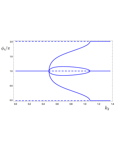
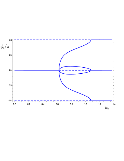
Figure 11: In these panels the various 4-site ($n=3$) multibreathers families in a chain with interaction range $r=3$ are shown. In the diagram we have considered $k_{2}$ variable, while $k_{3}=0.2$ in the left panel and $k_{3}=0.4$ in the right panel. The families depicted are qualitatively the same as the ones in the $n=3$, $r=2$ case. The only difference is that in the present case the value of ${k_{2}}_{cr}^{(1)}$ where the supercritical bifurcation occurs depends strongly on $k_{3}$ while the value of ${k_{2}}_{cr}^{(2)}$ where the subcritical bifurcation occurs remains almost fixed.

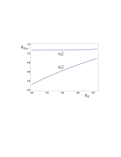
Figure 12: The values of the two ${k_{2}}_{cr}$, where the bifurcations occur, with respect to $k_{3}$. Although ${k_{2}}_{cr}^{(1)}$ depends strongly on $k_{3}$, ${k_{2}}_{cr}^{(2)}$ remains almost constant at ${k_{2}}_{cr}^{(2)}\simeq 1.075$.

VII 4-site breathers in a 2D square lattice with $r=2$

We now turn our considerations to the case of a square lattice, as the one in Fig. 13, with nearest-neighbor interactions, not only with the horizontal and vertical neighbors, but with the diagonal as well. The latter interaction is assumed to have a strength $\epsilon_{2}=k\epsilon_{1}$ (where $\epsilon_{1}\equiv\epsilon$ will be taken to denote the coupling strength of adjacent nodes along the lattice axes).

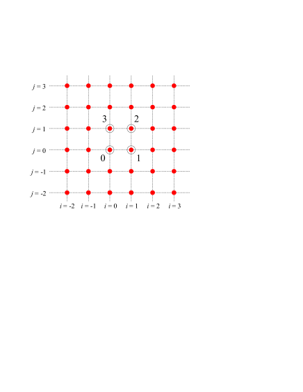
Figure 13: In the square lattice under consideration each oscillator is coupled with its neighbour not only in the horizontal and vertical directions but in the diagonal directions as well. So, every lattice site interacts with its 8 neighbours instead of the 4 of the classical KG square lattice configuration. In this setting, we consider 4-site breathers. Let the encircled oscillators in the figure be the central oscillators which are denoted as 0, 1, 2, 3 respectively

The Hamiltonian for this system is

$$\begin{array}[]{cll}H&=\displaystyle\sum_{i=-\infty}^{\infty}\sum_{j=-\infty}^{\infty}\left[\frac{1}{2}p_{ij}^{2}+V(x_{ij})\right]&+\displaystyle\frac{\varepsilon_{1}}{2}\sum_{i=-\infty}^{\infty}\sum_{j=-\infty}^{\infty}\left[(x_{ij}-x_{i-1,j})^{2}+(x_{ij}-x_{i,j-1})^{2}\right]\\ &&+\displaystyle\frac{\varepsilon_{2}}{2}\sum_{i=-\infty}^{\infty}\sum_{j=-\infty}^{\infty}\left[(x_{ij}-x_{i-1,j-1})^{2}+(x_{ij}-x_{i-1,j+1})^{2}\right]\end{array}$$ (26)

or

$$\begin{array}[]{cl}H=H_{0}+\varepsilon H_{1}&=\displaystyle\sum_{i=-\infty}^{\infty}\sum_{j=-\infty}^{\infty}\left[\frac{1}{2}p_{ij}^{2}+V(x_{ij})\right]+\\ &+\displaystyle\frac{\varepsilon}{2}\sum_{i=-\infty}^{\infty}\sum_{j=-\infty}^{\infty}\left\{(x_{ij}-x_{i-1,j})^{2}+(x_{ij}-x_{i,j-1})^{2}+\displaystyle k\left[(x_{ij}-x_{i-1,j-1})^{2}+(x_{ij}-x_{i-1,j+1})^{2}\right]\right\}\end{array}$$ (27)

We consider 4 “central” oscillators in the anti-continuum limit and we denote them by 0, 1,2 ,3 as it is shown in fig.13. We have then $\phi_{1}=w_{1}-w_{0}$, $\phi_{2}=w_{2}-w_{1}$, $\phi_{3}=w_{3}-w_{2}$ and $\phi_{4}=w_{0}-w_{3}$. But since, by construction, we have $\phi_{4}=2\pi-\phi_{1}-\phi_{2}-\phi_{3}$, we have finally only 3 independent $\phi_{i}$’s. The $\langle H_{1}\rangle$ in this case is

$$\begin{array}[]{l}\displaystyle\langle H_{1}\rangle=-\frac{1}{2}\sum_{m=1}^{\infty}A_{m}^{2}\left\{\cos(m\phi_{1})+\cos(m\phi_{2})+\cos(m\phi_{3})+\cos[m(\phi_{1}+\phi_{2}+\phi_{3})]\right.\\[8.0pt] \qquad\qquad\qquad\qquad\quad\left.+k\{\cos[m(\phi_{1}+\phi_{2})]+\cos[m(\phi_{2}+\phi_{3})]\}\right\}\end{array}$$

and the corresponding persistence conditions are

$$\begin{array}[]{ccl}M(\phi_{1})+M(\phi_{1}+\phi_{2}+\phi_{3})+k\,M(\phi_{1}+\phi_{2})&=&0\\[8.0pt] M(\phi_{2})+M(\phi_{1}+\phi_{2}+\phi_{3})+k[M(\phi_{1}+\phi_{2})+M(\phi_{2}+\phi_{3})]&=&0\\[8.0pt] M(\phi_{3})+M(\phi_{1}+\phi_{2}+\phi_{3})]+k\,M(\phi_{2}+\phi_{3})&=&0\end{array}$$

This case coincides with the 1D 4-site $r=3$ chain case, with $k_{3}=k_{1}=1$ and $k_{2}=k$. Hence, the results (both for the persistence and the stability of the solutions) are a special case of the previous section. All the existing multibreather families of this configuration are depicted in fig. 14.

In this diagram we can observe the appearance of {$\phi_{1}=\phi_{2}=\phi_{3}=\pi/2$} family, which is the vortex solution of the classical square Klein-Gordon lattice; see e.g., the relevant discussion in IJBC . In addition, there are several phase-shift families, the stability of which will be analyzed below. Interestingly, all these phase-shift breathers cease to exist at a critical value of $k=k_{cr}^{(2)}=1.03549$ except of the vortex one.

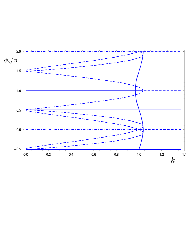
Figure 14: In this diagram, the various multibreather families of the square lattice configuration, are depicted. The value of $k$ determines the strength of the coupling in the diagonal direction. For a more detailed description of the particular families one can also refer to Fig. 15.

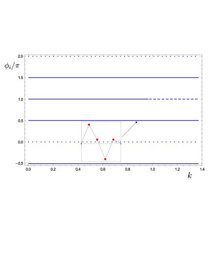
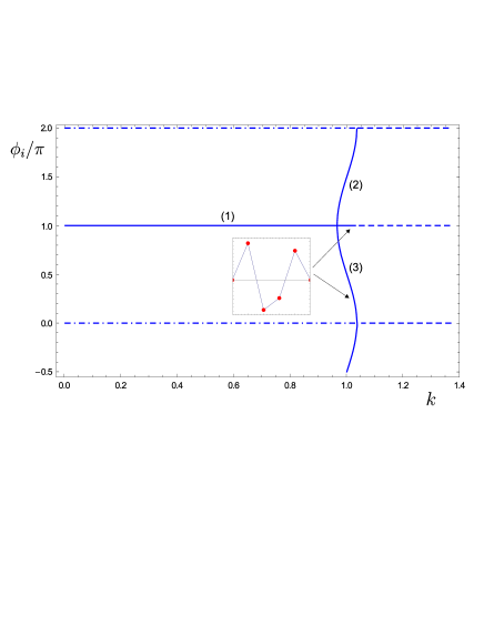
(a)		(b)
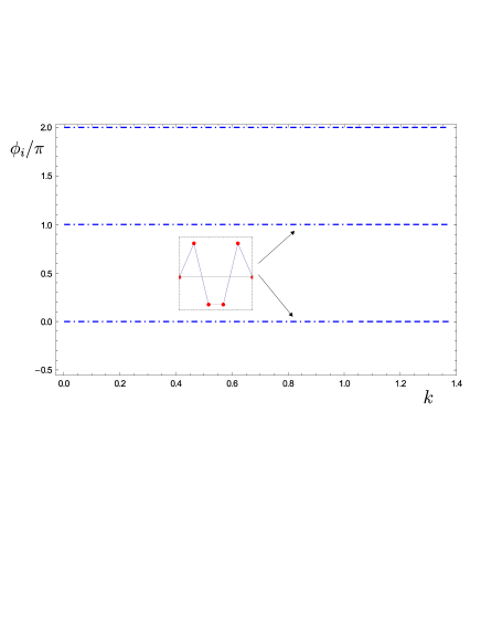
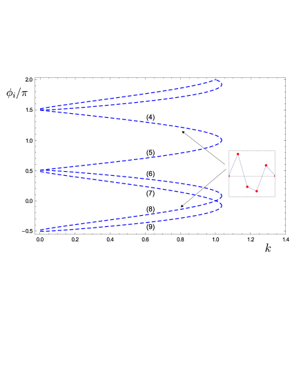
(c)		(d)

Figure 15: The various multibreather families that consist Fig. 14 are depicted. Portraits of the configuration of the central oscillators for the different multibreather families are shown as insets in the corresponding diagrams. Note that, for better presentation, instead of showing the the 4 central oscillators in a square configuration, we show their 1D equivalent. The line (or curve) type in the figures depends on the number of positive ${\chi_{z}}$ the corresponding family possesses: no positive ${\chi_{z}}$ corresponds to solid line, 1 positive ${\chi_{z}}$ corresponds to dashed line, 2 to dashed-dotted and 3 to dotted line. In (a) three families are shown. The first family is the in-phase one {$\phi_{1}=\phi_{2}=\phi_{3}=0\ \text{or}\ 2\pi$}, which possesses 3 positive ${\chi_{z}}$. The second family is the vortex {$\phi_{1}=\phi_{2}=\phi_{3}=\pi/2\ (\text{or}\ 3\pi/2)$} family. It possesses no positive ${\chi_{z}}$. The third family is the anti-phase one {$\phi_{1}=\phi_{2}=\phi_{3}=\pi$}. This family possesses no positive ${\chi_{z}}$ for $k<k_{cr}^{(1)}=0.96572$, while for $k>k_{cr}^{(1)}$ it acquires 2 positive ${\chi_{z}}$. At this point it bifurcates to provide the phase-shift 1 family. In this figure only the inset of the vortex family is present because all the others are the same as the ones presented for the equivalent 1D configuration, in figs. 10. In (b) the phase-shift 1 {$\phi_{1}=\phi_{3}=\pi$, $\phi_{2}=\phi$} family is shown, which exists for $k_{cr}^{(1)}<k<k_{cr}^{(3)}=1.03549$. It is depicted by $\phi_{1}=\phi_{3}=(1)$ and $\phi_{2}=(2)$ or $\phi_{1}=\phi_{3}=(1)$ and $\phi_{2}=(3)$. It possesses no positive ${\chi_{z}}$ for $k_{cr}^{(1)}<k<k_{cr}^{(2)}=1.0344$. At $k=k_{cr}^{(2)}$ it collides with the phase-shift 2 family. For $k_{cr}^{(2)}<k<k_{cr}^{(3)}$ the family possesses 1 positive ${\chi_{z}}$. At $k=k_{cr}^{(3)}$ it collides with the mixed family. In (c) the mixed family {$\phi_{1}=\phi_{3}=\pi$, $\phi_{2}=0$} is depicted. It has 2 positive ${\chi_{z}}$ for $k<k_{cr}^{(2)}$ and 1 positive ${\chi_{z}}$ for $k_{2}>k_{cr}^{(3)}$. Finally in (d) two phase-shift families are depicted. The phase phase-shift 2a family, which is represented by $\phi_{1}=\phi_{3}=(4)$ and $\phi_{2}=$(8) which collides with the $\phi_{1}=\phi_{3}=(5)$ and $\phi_{2}=$(6) for $k_{2}=k_{cr}^{(2)}$, and the phase-shift 2b family which is represented by $\phi_{1}=\phi_{3}=(4)$ and $\phi_{2}=$(9) which collides with the $\phi_{1}=\phi_{3}=(5)$ and $\phi_{2}=$(7) for $k_{2}=k_{cr}^{(2)}$. They both possess 1 positive ${\chi_{z}}$.

The mutibreather families that are supported by the present configuration are described in what follows.

• {$\phi_{1}=\phi_{2}=\phi_{3}=0$} (in-phase) It is shown in Fig.15(a). It possesses 3 positive ${\chi_{z}}$ independently of the value of $k_{2}$.

• {$\phi_{1}=\phi_{2}=\phi_{3}=\pi/2$} (vortex). It is shown in Fig.15(a). It has no positive ${\chi_{z}}$ independently of the value of $k_{2}$ and does not interact (i.e., collide) with any other family of solutions.

• {$\phi_{1}=\phi_{2}=\phi_{3}=\pi$} (anti-phase). It is shown in Fig.15(a). It has no positive ${\chi_{z}}$ for $k<k_{cr}^{(1)}=0.96572$, while for $k>k_{cr}^{(1)}$ it acquires 2 positive ${\chi_{z}}$.

• {$\phi_{1}=\phi_{3}=\pi$, $\phi_{2}=\phi$} (phase-shift 1). It is represented by in Fig.15(b) $\phi_{1}=\phi_{3}=(1)$ and $\phi_{2}=(2)$ or $\phi_{1}=\phi_{3}=(1)$ and $\phi_{2}=(3)$. It exists for $k_{cr}^{(1)}<k_{2}<k_{cr}^{(3)}$. It bifurcates from the anti-phase family at $k=k_{cr}^{(1)}$ and possesses 3 negative ${\chi_{z}}$ for $k_{cr}^{(1)}<k<k_{cr}^{(2)}=1.0344$. At $k_{2}=k_{cr}^{(2)}$ it collides with the phase-shift 2 family in a bubcritical pitchfork bifurcation. So, for $k_{cr}^{(2)}<k<k_{cr}^{(3)}$ it possesses 2 negative and a positive ${\chi_{z}}$. At $k=k_{cr}^{(3)}$ it collides with the mixed family.

• {$\phi_{1}=\phi_{3}=\pi$, $\phi_{2}=0$} (mixed). It is shown in Fig.15(c). It has 2 positive ${\chi_{z}}$ for $k<k_{cr}^{(3)}=1.0355$ and 1 positive ${\chi_{z}}$ for $k_{2}>k_{cr}^{(3)}$.

• (phase-shift 2a) It is represented in Fig.15(d) by $\phi_{1}=\phi_{3}=(4)$ and $\phi_{2}=$(8) which collides with the $\phi_{1}=\phi_{3}=(5)$ and $\phi_{2}=$(6) for $k_{2}=k_{cr}^{(2)}$ and have 1 positive ${\chi_{z}}$.

• (phase-shift 2b) It is represented in Fig.15(d) by $\phi_{1}=\phi_{3}=(4)$ and $\phi_{2}=$(9) which collides with the $\phi_{1}=\phi_{3}=(5)$ and $\phi_{2}=$(7) for $k_{2}=k_{cr}^{(2)}$ and have 1 positive ${\chi_{z}}$.

Notes on Figs. 14 and 15:

1. At $k=k_{cr}^{(2)}$ the $\phi_{2}=(3)$ branch of the phase-shift 1 family collides with the phase-shift 2a family, while the the $\phi_{2}=(2)$ branch of the phase-shift 1 family collides with the symmetric (and equivalent) of branches $\phi_{2}=(7)$ and $\phi_{2}=(9)$ of the phase-shift 2b family.

2. At $k=0$ the phase-shift 2 family approaches very much the vortex family, so it is plausible to expect that at that point they coincide. Yet, there is a small difference in the values of $\phi_{i}$ of the two families due to the nonlinear character of the oscillators constituting the lattice, i.e., due to the existence of an infinity of terms in the development (3). For a smaller frequency of oscillation, the nonlinear character of the oscillation becomes stronger, hence the terms after the first in (3) become larger and the two families are more clearly separated.

VIII Discussion - Comparison with the DNLS results

It should be noted here that a number of results similar to the ones presented herein have been recently presented in the context of the DNLS equation e.g. in pgkpla ; chong . The setting of the DNLS essentially reflects a special case example of our Klein-Gordon calculation where instead of the existence and stability conditions reflecting a sum over all the harmonics due to the U$(1)$ invariance of the underlying model, only the first harmonic is present. Nevertheless, the latter is sufficient to induce a number of the conclusions that we inferred herein. In particular, next-nearest neighbor interactions create phase-shift multibreathers (which were also parallelized to discrete vortex breathers in hexagonal lattices), as illustrated in pgkpla . As also shown in the same work, the long range interactions may drastically affect the stability properties of two-dimensional discrete vortices (in square lattices). On the other hand, the work of chong provided a different analytical handle, via variational approximations, on the solutions that arise in settings with long range interactions. Furthermore, it was able to capture phenomena (both analytically and numerically) such as the supercritical or subcritical pitchfork bifurcations for such phase-shift multibreather solutions with NNN interactions. For instance, in the DNLS case the supecritical bifurcation leading to the emergence of such solutions would happen precisely at $k=0.5$ (due to the relevance of just the first harmonic) and not at $k=0.48286$ as obtained here in section IV B for the Klein-Gordon case. Nevertheless, the basic phenomenology remains intact.

IX Conclusions

Classical Klein-Gordon chain with nearest neighbor interactions support multibreather solutions only with phase differences between successive oscillators of $\phi_{i}=0,\pi$. There, the stability scenaria are specific and well known. For a KG chain with $P=\varepsilon\frac{\partial\omega}{\partial J}<0$ the anti-phase configuration is the only stable one, while for $P=\varepsilon\frac{\partial\omega}{\partial J}>0$ the in-phase configuration is the only stable multibreather solution.

On the other hand, in chains with long range interactions the picture is substantially different. First of all, in such chains, multibreathers with $\phi_{i}\neq 0,\pi$ (phase-shift multibreathers) can be supported in addition to the standard $\phi_{i}=0,\pi$ ones. The existence of phase-shift multibreathers as well as the specific $\phi_{i}$’s of such profiles depend on the various coupling parameters $\varepsilon_{i}$ within the chain. There are critical values of $k_{i}=\varepsilon_{i}/\varepsilon_{1}$ past which a bifurcation occurs (typically a supercritical pitchfork) and phase shift breathers begin to exist. Past this bifurcation point, the stability properties of the existing multibreathers are significantly modified, although this also depends on the particular (soft or hard) nature of the nonlinearity. As, however, additional parameters are tuned (e.g., higher ranges of neighbor interactions), it is also possible for such phase-shift solutions to terminate in subcritical pitchfork bifurcations.

These results are not unique to the realm of one-dimensional lattices with higher range of interactions. They can also be developed for two-dimensional square lattices in which case they may lead to bifurcations or terminations of the families of discrete vortices which arise therein. Such vortices sustained by the two-dimensional analogs of the lattice can be of either a symmetric or asymmetric type. In particular, in the case considered herein, the presence of diagonal coupling within the square was critical in inducing the emergence of asymmetric such patterns.

This study opens a number of a directions for further investigation. Firstly, it would be very relevant to examine particular functional forms of the decay of the long range interactions (e.g., exponentially or polynomially decaying ones) to identify whether any systematic conclusions can be derived on the basis of such decay laws. Secondly, it would also be very interesting to examine the interplay of the geometry of higher dimensional lattices (and the interactions that they present) with the strength of the long range interactions that can be considered therein and to try to derive some general conclusions about the possible stable/unstable discrete soliton and discrete vortex solutions. Finally, an important and immediate direction that can be followed with the results of the paper in hand could be the effect of long-range interaction in phase-shift phonobreathers, whose stability for nearest-neighbor interaction was considered in CAR11 . A physical application of relevance and worthwhile of further investigation concerns the biological models for DNA CAGR02 ; CSAH04 or protein alpha-helices AGCC02 , where dipole long-range interactions are relevant.

- [1] http://users.auth.gr/vkouk/lri/videos.zip.
- [2] T. Ahn, R. S. MacKay, and J.-A. Sepulchre. Dynamics of relative phases: Generalised multibreathers. Nonlinear Dynamics, 25:157–182, 2001.
- [3] J. F. R. Archilla, J. Cuevas, B. Sánchez-Rey, and A. Álvarez. Demonstration of the stability or instability of multibreathers at low coupling. Physica D, 180:235, 2003.
- [4] J. F. R. Archilla, Yu. B. Gaididei, P. L. Christiansen, and J. Cuevas. Stationary and moving breathers in a simplified model of curved alpha helix proteins. J. Phys. A.: Math. Gen., 35:8885, 2002.
- [5] S. Aubry. Breathers in nonlinear lattices: existence, linear stability and quantization. Physica D, 103:201–250, 1997.
- [6] G. Bartal, O. Cohen, T. Schwartz, O. Manela, Fredman B., M. Segev, H. Buljan, and N. K. Efremidis. Spatial photonics in nonlinear waveguide arrays. Opt. Express, 13:1780, 2005.
- [7] C. Chong, R. Carretero-Gonzalez, B. A. Malomed, and P. G. Kevrekidis. Variational approximations in discrete nonlinear Schrödinger equations with next-nearest-neighbor couplings. Physica D, 240:1205, 2011.
- [8] J. Cuevas, J. F. R. Archilla, Yu. B. Gaididei, and F. R. Romero. Moving breathers in a DNA model with competing short- and long-range dispersive interactions. Physica D, 163:106–126, 2002.
- [9] J. Cuevas, J. F. R. Archilla, and F. R. Romero. Effect of the introduction of impurities on the stability properties of multibreathers. Nonlinearity, 18:76, 2005.
- [10] J. Cuevas, J. F. R. Archilla, and F. R. Romero. Stability of non-time-reversible phonobreathers. J. Phys. A.: Math. Theor., 44:035102, 2011.
- [11] J. Cuevas, V. Koukouloyannis, P. G. Kevrekidis, and J. F. R. Archilla. Multibreather and vortex breather stability in Klein–Gordon lattices: Equivalence between two different approaches. Int. J. Bifur. Chaos, 21:2161, 2011.
- [12] J. Cuevas, E. B. Starikov, J. F. R. Archilla, and D. Hennig. Moving breathers in bent DNA with realistic parameters. Mod. Phys. Lett. B, 18:1319–1326, 2004.
- [13] N. K. Efremidis. Discrete solitons in nonlinear zigzag optical waveguide arrays with tailored diffraction properties. Phys. Rev. E, 65:056607, 2002.
- [14] M. Feckan and V. M. Rothos. Travelling waves of discrete nonlinear Schrödinger equations with nonlocal interactions. Applicable Analysis, 89:1387–1411, 2010.
- [15] S. Flach and A. V. Gorbach. Discrete breathers - Advances in theory and applications. Phys. Rep., 467:1, 2008.
- [16] S. Flach and C. R. Willis. Discrete breathers. Phys. Rep., 295:182, 1998.
- [17] P. G. Kevrekidis. The discrete nonlinear Schrödinger equation. Springer-Verlag, Berlin, 2009.
- [18] P. G. Kevrekidis. Non-nearest-neighbor interactions in nonlinear dynamical lattices. Phys. Lett. A, 373:3688, 2009.
- [19] Yu. S. Kivshar and G. P. Agrawal. Optical solitons: from fibers to photonic crystals. Academic Press, San Diego, 2003.
- [20] V. Koukouloyannis. Non-existence of phase-shift multibreathers in one-dimensional klein-gordon lattices with nearest-neighbor interactions. ArXiV:1204.4929, 2012.
- [21] V. Koukouloyannis and S. Ichtiaroglou. Existence of multibreathers in chains of coupled one-dimensional hamiltonian oscillators. Physical Review E - Statistical, Nonlinear, and Soft Matter Physics, 66(6):066602, 2002.
- [22] V. Koukouloyannis and P. G. Kevrekidis. On the stability of multibreathers in Klein–Gordon chains. Nonlinearity, 22:2269, 2009.
- [23] V. Koukouloyannis, P. G. Kevrekidis, K. J. H. Law, I. Kourakis, and D. J. Frantzeskakis. Existence and stability of multisite breathers in honeycomb and hexagonal lattices. J. Phys. A: Math. Theor., 43:235101, 2010.
- [24] V. Koukouloyannis and R. S. MacKay. Existence and stability of 3-site breathers in a triangular lattice. J. Phys. A: Math. Gen., 38:1021, 2005.
- [25] F. Lederer, G. I. Stegeman, D.N. Christodoulides, G. Assanto, M. Segev, and Y. Silberberg. Discrete solitons in optics. Phys. Rep., 463:1, 2008.
- [26] R. S. MacKay. Discrete breathers: classical and quantum. Physica A, 288:174–198, 2000.
- [27] R. S. MacKay. Slow manifolds. In T. Dauxois, A. Litvak-Hinenzon, R. S. MacKay, and A. Spanoudaki, editors, Energy Localisation and Transfer, pages 149–192. World Scientific, 2004.
- [28] R. S. MacKay and S. Aubry. Proof of the existence of breathers for time-reversible or Hamiltonian networks of weakly coupled oscillators. Nonlinearity, 7:1623, 1994.
- [29] R. S. MacKay and J.-A. Sepulchre. Effective Hamiltonian for travelling discrete breathers. Journal of Physics A, 35:3985–4002, 2002.
- [30] O. Morsch and M. O. Oberthaler. Dynamics of bose-einstein condensates in optical lattices. Rev. Mod. Phys., 78:179, 2006.
- [31] J. B. Page. Asymptotic solutions for localized vibrational modes in strongly anharmonic periodic systems. Phys. Rev. B, 41:7835, 1990.
- [32] D. E. Pelinovsky and A. Sakovich. Multi-site breathers in Klein-Gordon lattices: stability, resonances and bifurcations. ArXiV:1111.2557, 2011.
- [33] M. Peyrard. Nonlinear dynamics and statistical mechanics of DNA. Nonlinearity, 17:R1, 2004.
- [34] M. Sato, B. E. Hubbard, and A. J. Sievers. Nonlinear energy localization and its manipulation in micromechanical oscillator arrays. Rev. Mod. Phys., 78:137, 2006.
- [35] S. Sen, J. Hong, J. Bang, E. Avalos, and E. Doney. Solitary waves in the granular chain. Phys. Rep., 462:21, 2008.
- [36] J.-A. Sepulchre and R. S. MacKay. Localized oscillations in conservative or dissipative networks of weakly coupled autonomous oscillators. Nonlinearity, 10(3):679–713, 1997.
- [37] A. J. Sievers and S. Takeno. Intrinsic localized modes in anharmonic crystals. Physical Review Letters, 61:970–973, 1988.
- [38] K. Yoshimura. Existence and stability of discrete breathers in diatomic fermi-pasta-ulam type lattices. Nonlinearity, 24:293, 2011.