Deflation and Flexible SAP-Preconditioning of GMRES in Lattice QCD Simulation
Abstract
The simulation of lattice QCD on massively parallel computers stimulated the development of scalable algorithms for the solution of sparse linear systems. We tackle the problem of the Wilson-Dirac operator inversion by combining a Schwarz alternating procedure (SAP) in multiplicative form with a flexible variant of the GMRES-DR algorithm. We show that restarted GMRES is not able to converge when the system is poorly conditioned. By adding deflation in the form of the FGMRES-DR algorithm, an important fraction of the information produced by the iterates is kept between successive restarts leading to convergence in cases in which FGMRES stagnates.
1 Introduction
The simulation of Lattice QCD is among one of the most challenging problems in computational science because of its enormous computational cost, see [1], e.g.. With sufficiently powerful computers becoming available during the last fifteen years, the simulation of Lattice QCD including dynamical fermions became a reality. The de-facto standard algorithm used to accomplish this task is the Hybrid Monte Carlo (HMC) algorithm [2]. HMC introduces a fictious time, in which a dynamical system is evolved according to the system Hamiltonian. In order to integrate the Hamiltonian equations of motion, the forces due to both, gauge field and pseudo-fermion field, have to be evaluated accurately. The by far most demanding numerical task is the inversion of the fermionic Dirac matrix, needed to evaluate the fermion force. In this paper we investigate a class of inverters for the fermionic Dirac matrix which is particularly well adapted to current high performance hardware architecture. Our work was primarily inspired by the architecture of the QPACE machine, see [3, 4], but it is of a general nature and applies to all architectures were data movements rather than arithmetic operations tend to be the limiting factor on performance.
The development of machine-aware algorithms has become particularly important during the last years as computer architectures move towards dramatically increased floating point (FP) speed and increased on-chip parallelism. For reasons of cost and because of physical limitations, these improvements are not accompanied by comparable progresses in the bandwidths and latencies of main memory and processor interconnects. It is predicted that this situation will be even aggravated as we move towards the Exascale area, see [5], e.g..
An often used rough indicator of balance between processor and memory subsystems is the ratio between peak main memory bandwidth and peak floating point performance. In the past few years this value went down from to and less for the CELL processor, modern GPUs and general purpose x86 systems. This increasing gap is the main reason for a line of computer science research on software techniques aimed at maximizing cache utilization. A famous example is [6].
The algorithm cost evaluation must take into account not only the FP operations (as it was traditionally done some years ago when FP was the most relevant bottleneck in numerical applications), but has to carefully evaluate the amount and pattern of data movement among the levels of memory hierarchy and the network as these are now the most limiting factors.
Algorithms that are more suitable for these increasingly unbalanced computer architectures are particularly attractive as they can give easier access to the FP performances offered today.
We describe an algorithm for the Dirac-Wilson matrix inversion that is able to exploit the architectural features of modern machines. We show the convergence behaviour and demonstrate the performance with our implementation on the peculiar SFB-TR55 QPACE architecture based on the IBM PowerXCell8i processor with state of the art lattices.
2 Domain decomposition and SAP
The Wilson fermion matrix [7] describes a (periodic) nearest neighbor coupling on the 4-dimensional space-time lattice. Without further explanation, our desire is to solve the linear system
Owed to the complexity and size of , a direct solution is not feasible and we therefore exploit the structure of . We decompose the overall lattice into sublattices, called domains. For each domain, we obtain a local Wilson fermion operator by simple restriction; at the local boundary of a domain, we remove the couplings with neighboring domains. To describe this formally, let stand for a 4-tupel describing a lattice site and let denote the overall lattice. The Dirac Wilson operator can then be written as
| (1) |
where is to be taken mod .
A domain is characterized by the bounds for its lattice sites which are given by . The local Dirac operator for domain is thus given as
| (2) |
where indicates that the sum is to be taken only over those contributions for which or is in .
Assuming that the local Wilson operators are easy to invert, we can perform the following basic domain decomposition iteration, known as the multiplicative Schwarz method in the domain decomposition literature [8, 9].
Herein, the superscript indicates that we only take the part which corresponds to the subdomain . Due to the nearest neighbor coupling of , computing is a local operation which involves only those components of which belong to subdomain , i.e. and those from neighboring subdomains which are at the boundary to domain .
If we use a red-black coloring of the subdomains as depicted in Fig. 1 for a two-dimensional lattice, and we have an even number of sub-domains in each dimension of the lattice, then there is no coupling between subdomains of the same color. When we order all red (say) domains first, we see that in the algorithm above the values of the residual does not depend on whether or not we updated the part of the iterate for the other subdomains of the same color. If we proceed by colors, we end up with the following variant of the basic domain decomposition iteration which is termed the Schwarz alternating procedure (SAP) in [10].
3 SAP in computational practice
In computational practice, the SAP method can rarely be used directly in the form given by Algorithm 2. On one hand it is usually too costly to solve the local systems exactly. One rather computes an approximation to using another, inner iterative method on the systems . Usually, the fastest overall method arises if one requires a fairly low accuracy in the inner iteration. For example, one requires that the approximate solution reduces the initial residual by just a factor of 10, i.e. one requires
Such a method is termed an inexact SAP method.
On the other hand, even the exact SAP iteration may diverge for the Wilson Dirac operator when the hopping parameter approaches the critical value . Indeed, most of the convergence theory for multiplicative Schwarz methods assumes that the operator is hermitian and positive definite, see [8, 9], which is not the case for the Wilson Dirac operator.
The usage of SAP methods is particularly suitable on parallel machines and in general on machines with a memory hierarchy. Provided that at least two subdomains are assigned to a machine node, there is no need for network communication during the solution of the Wilson equation on the subdomains, since all the necessary data is on the node. Data only needs to be communicated for the update of the residual. In practice, there are more than two subdomains per node giving the possibility to overlap network communication and computation. The required network bandwidth, and in particular latency, is less stringent than for a simple Krylov solver, since the approximate solution of the subdomain Wilson equation requires some iterations. The required machine performance on global network operations (i.e. global sum, barrier, etc.) is also typically reduced, since the frequency of such operations is lower than in the case of a Krylov solver. We have chosen SAP as a preconditioner to be used on the most time-critical solves on our machine QPACE. The QPACE torus network [4] is designed with a typical Krylov solver in mind and has therefore high bandwidth and low latency, nevertheless SAP is particularly appealing due to the peculiar memory hierarchy architecture of the IBM PowerXCell 8i Processor. On this processor, the fast on-chip memory is not managed automatically by the hardware as on standard processors (cache), but its control is completely left to the programmer. If the size of the subdomain is chosen such that it fits the fast memory, no main memory access is necessary for the subdomain solve, giving the possibility to achieve impressive sustained performance for the subdomain solves (up to 50% of the peak) [11], [12]. This feature of the SAP algorithm is interesting also for future architectures as the main memory performance will continue to improve at a lower rate than processor performance.
4 Domain decomposition preconditioner
Exact or inexact SAP iterations can be used as a preconditioner in a Krylov subspace method like GMRES [13] or GCR [14]. This will usually result in an iterative process which converges faster than the Krylov subspace method without preconditioning or the stand-alone SAP iteration. We will discuss GMRES and GCR in quite some detail later in section 5. At this point, we concentrate on aspects pertaining to the use of inexact SAP iterations in the context of preconditioning.
Loosely speaking, the speed of convergence of a Krylov subspace method for a generic system
gets faster the closer is to the identity. So, to accelerate the convergence one tries to construct (or implicitly use) a matrix , the preconditioner, such that the matrix of the (right) preconditioned system
is close to the identity. In this sense, should be an approximation to the inverse of . Such is given implicitly if we perform some steps of an iterative procedure like SAP.
Each step of the Krylov subspace method requires one multiplication with and one with . If we perform exact SAP with a fixed number, say, of iterative steps, the preconditioner can be expressed as the truncated series
where the matrices and result from a splitting of the matrix . To be specific, for the SAP iteration from Algorithm 2, where , this splitting is based on the red-black permuted matrix given as
Herein, the blocks and are made up of all the local Dirac operators of the black and the red subdomains, respectively and the off-diagonal blocks contain the couplings between subdomains of different color. Then
In inexact SAP we invert only approximately, using some inner iteration on the diagonal blocks . If this inner iteration is non-stationary, as it is the case if we perform some steps of GMRES or MR [15], the implicitly given preconditioner changes at each iteration. This is a fact one has to account for when formulating the preconditioned Krylov subspace methods. In the linear algebra literature such methods are termed flexible, see [16, 15] since they adapt themselves to situations where the preconditioner varies from one iteration to the next.
The next chapter will first introduce the flexible restarted GMRES method before turning to the crucial subject of this paper, namely its acceleration via deflation.
5 F-GMRES-DR
To simplify the presentation we will use a generic notation in this chapter, i.e. the linear system to solve will be denoted
A preconditioner will be denoted . In a variable preconditioning context, where the preconditioner will depend on the current iterative step , we denote the preconditioner by . Note that will usually not be given explicitly but rather be the result of some steps of a non-stationary iteration like inexact SAP.
Particular aspects for (inexact) SAP preconditioning of the Wilson Dirac operator will be discussed later.
5.1 GMRES and GCR
We consider a generic non-singular linear system
Given an initial guess and its residual , the -th Krylov subspace is defined as
For ease of notation, we will often write instead of . It is known that the solution is contained in the space where denotes the smallest for which . Krylov subspace methods work by iteratively choosing approximations from to approximate . The GMRES and GCR method are Krylov subspace methods which both obtain the “optimal” in the sense that the residual satisfies the minimal residual condition
Note that for any subspace of we have
| (3) |
where is the residual of . The equivalence (3) holds because the minimizer is such that represents the orthogonal projection of onto . So the minimal residual condition for GMRES or GCR is equivalent to
| (4) |
GMRES works by building a sequence of orthonormal vectors which span . The coefficients in are then obtained by solving a small least squares problem. GCR computes a sequence of orthonormal vectors which span , and an auxiliary sequence with . The iterate is obtained by an update . Both, GMRES and GCR, suffer from the fact that the number of vectors stored and the cost for the orthogonalizations increase linearly with . A remedy is to restart or truncate the methods. GCR requires twice as many vectors to store as GMRES, and its total arithmetic costs are slightly higher than in GMRES. If convergence is slow, GMRES is significantly more stable numerically than GCR as was proven in [17]. There is one advantage of GCR over GMRES, however: While the GMRES algorithm has to be modified (slightly) to allow for variable preconditioning, GCR adapts itself “automatically” to such a situation. For this reason GCR was used in various contexts of variable preconditioners like, for example, [10]. In the present paper we consider situations where there is an additional need for (inexact) deflation in order to get sufficiently fast convergence. While this can be done elegantly and efficiently within the GMRES framework, there seems to be no such way for GCR. This explains why we focus on GMRES from now on.
5.2 Flexible GMRES
Standard (non-variable) right preconditioning of the equation means that instead of looking for an iterate we now look for one in the space , where stands for the preconditioning matrix. The idea is that with a good preconditioner (a good approximation to ), the “search space” contains substantially better approximations to the solution than . In right preconditioned GMRES [15] we obtain the -th iterate as
| (5) |
Right preconditioned GMRES uses the Arnoldi process to compute an orthonormal basis of , orthogonalizing against all previous vectors . The solution of (5) can then be obtained as the solution of a small least squares problem. We do not discuss this further here, since right preconditioned GMRES appears as a special case of flexible GMRES [16] which we develop in all its details now.
In a flexible context, the preconditioning matrix depends on the iterative step, i.e. we have a new preconditioning matrix in each step . In a “flexible” Arnoldi process we thus orthogonalize against all previous vectors . It will turn out useful to also keep track of the preconditioned vectors for future use when computing (flexible) GMRES iterates. So we end up with the flexible Arnoldi process described as Algorithm 3.
The flexible Arnoldi relation
| (6) |
summarizes the computations of Algorithm 3, its -th column representing
Note that the matrix is upper Hessenberg, i.e. its elements below the first subdiagonal, for , are all 0. The columns of are orthonormal, so we have .
In the non-flexible case, i.e. for all , the orthonormal vectors span the Krylov subspace , and the vectors span the search space . In this case we can formulate (6) without to retrieve the standard Arnoldi relation
| (7) |
In the case of a variable preconditioner, there is no immediate notion of a (preconditioned) Krylov subspace, but we can still use the space spanned by the vectors , i.e. as a search space. This is the approach taken in flexible GMRES (F-GMRES) [16], where we obtain the iterates by imposing the minimal residual condition for . So we have to compute
| (8) |
Using the flexible Arnoldi relation (6) and the fact that has orthonormal columns, we have
So solving the least squares problem gives the coefficient vector from which we retrieve the FGMRES iterate as
We note in passing that the least squares problem is usually solved via a QR-factorization of . Due to the upper Hessenberg structure of , this can easily be done in an iterative manner by updating the QR-decomposition of to that of using one additional Givens rotation. Moreover, it is possible to very cheaply update the norm of the residual of the -th GMRES iterate without explicitly computing the iterate. This can be used to implement an early termination criterion in cases where the -th (F)GMRES iterate is already accurate enough for . Details can be found in [15], e.g.. See also section 5.6.
5.3 Restarts and Deflation
If larger values of are required to obtain a sufficiently accurate approximation , full F-GMRES as described in the previous section is not feasible since we have to store the vectors and and the total cost for the orthogonalizations in the flexible Arnoldi process grow like . It is therefore common practice to use restarted F-GMRES. The integer is fixed to a moderate value. One then goes through several cycles. Each cycle performs steps of the full F-GMRES algorithm, with its initial guess given by the approximation to the solution computed in the previous cycle.
While restarts overcome problems with storage and computational complexity, they may severely degrade the convergence behaviour, and it might even happen that the method stagnates at a large residual norm without achieving any further progress. For difficult problems, this phenomenon has been widely observed in the literature, and several cures have been proposed. One of the most appropriate ones is the deflated restart modification which we discuss now.
Upon a restart, all the information contained in the search space built up so far is lost. In particular, in the new cycle we do not keep the residuals orthogonal to . The idea of deflated restarts is to extract a low-dimensional subspace of which contains the most important information in order to speed-up convergence, and to at least maintain the residuals orthogonal to . The new cycle can then be characterized as an augmenting Krylov subspace method with as the augmenting space. The crucial point is that, as we will see in the next section, it is possible to construct this deflating augmenting subspace in such a way that we do not need additional multiplications with .
5.4 Augmentation by Deflation
We first describe the ideas and technicalities of deflated restarts for the non-flexible case. The extension to FGMRES will be given in section 5.5. So for now we assume we have a fixed preconditioner in every iteration, and to further simplifiy the notation we base our whole discussion on the non-preconditioned system . The (right) preconditioned case is obtained by merely replacing with everywhere.
The presence of eigenvector components corresponding to small eigenvalues in a residual induces a large contribution of these eigenvectors in the error . It is thus desirable to chose the augmenting subspace as one that contains approximations to eigenvectors belonging to small eigenvalues. Those can be approximated from the Krylov subspace built up in the previous cycle. If this is done in the right manner, one can establish an Arnoldi type process for the augmented spaces with little additional cost as compared to standard Krylov subspaces, so that one ends up with an efficient method. We now give the details, following [18], which in turn builds on [19, 20, 21]. The key ingredient is to use harmonic Ritz vectors [22].
Definition 1
Given a matrix and a subspace , a harmonic Ritz pair with for with respect to satisfies
| (9) |
Harmonic Ritz pairs are well suited to approximate eigenpairs with a small eigenvalue [22]. The following lemma shows how harmonic Ritz pairs can be computed in cases where is a Krylov subspace or an appropriately augmented Krylov subspace.
Lemma 1
Let be a subspace of of dimension and assume that
Let the columns of be orthonormal vectors such that span and span , so that there exists a full rank matrix with
| (10) |
Moreover, let
Then:
-
a)
The harmonic Ritz pairs of w.r.t. are given as , where is an eigenpair of the matrix
-
b)
The residual of a harmonic Ritz pair satisfies
where spans the orthogonal complement of in , i.e.
Proof. Using (10), the defining property (9) for the Ritz pair with turns into
Since has full rank, the matrix is non-singular. The last equality can thus be further reduced to
which shows a). Part b) is trivial, since the residual of any harmonic Ritz pair is in and is orthogonal to .
So, to obtain harmonic Ritz pairs, we first compute as the solution of an linear system and then compute the eigenpairs of .
Note that by (3) the vector from part b) of Lemma 1 is also the residual of the GMRES iterate with respect to the search space . Since in the situation of Lemma 1 we have
| (12) |
for any subspace spanned by some harmonic Ritz vectors, we see that the augmented Krylov subspaces satisfy
This has two major consequences. The first is that, starting from an orthonormal basis of , we can build nested orthonormal bases for the spaces in an Arnoldi type manner. The second is that we can compute harmonic Ritz vectors with respect to in the way given in Lemma 1.
This is why we are able to set up a restarted GMRES method with deflation of harmonic Ritz vectors, where each cycle consists of the following steps:
-
1.
Extract harmonic Ritz pairs from the “search space” built in the previous cycle; these harmonic Ritz vectors span the current augmenting subspace .
-
2.
With denoting the residual of the iterate at the beginning of the current cycle, compute nested orthonormal bases for such that for we have the Arnoldi type relation
(13) -
3.
Compute the current GMRES iterate and its residual using (13).
Here, as in the sequel, we use the superscript to denote quantities from the previous cycle; no superscript refers to the current cycle. For an efficient implementation, all three steps are coupled by the way in which we construct the orthogonal basis for the current search space . We now discuss the three steps in detail.
Extracting the Ritz pairs
Let denote the matrix containing the orthonormal basis vectors of the search space built up in the previous cycle. By Lemma 1a), the harmonic Ritz vectors to augment the current Krylov subspace can be computed using from the Arnoldi-type relation (13) of the previous cycle. The harmonic Ritz vectors are then given as
which we summarize as
| (14) |
Computing the next GMRES iterate and its residual.
Assume that we have already built , the columns which represent an orthonormal basis of the current search space. We have to compute such that is minimal. The residual of the current iterate, which is in and thus in , can be expressed as
Taking (13) as granted for the moment, we have
Since the columns of are orthonormal, minimizing is therefore equivalent to solving the small least squares problem
This gives the next GMRES iterate with residual
| (15) |
Building the orthonormal basis for the current search space
The crucial part here is to obtain an orthonormal basis for without investing multiplications with .
From the columns of being orthonormal, we obtain an orthonormal basis of by computing an orthonormal basis for from (14), i.e. by computing the QR-factorization , where has orthonormal columns, and putting
From (4) we have , where is the residual of the iterate at the beginning of the current cycle, according to (15). Defining as
| (16) |
we thus have that . So we can extend to an orthonormal basis of by extending the QR-factorization to a QR factorization where
This gives the relation
| (17) |
On the other hand, by (12) for there exists a matrix such that
| (18) |
This matrix is actually given as
| (19) |
which can be seen by comparing
which follows from the Arnoldi relation of the previous cycle and
which is due to (17) and (18). We have therefore shown (13) for .
The Arnoldi-type relation (18) for an orthonormal basis of can now be extended to an orthonormal basis of through the standard Arnoldi orthogonalization procedure, where in step we orthogonalize against all previous basis vectors. As a consequence, the matrices in the resulting Arnoldi-type relation (13) have the form
which has upper Hessenberg structure except for the first rows. Herein, is from (19); for the other entries see Algorithm 4 below.
5.5 Deflating flexible GMRES
If we use a constant preconditioner , the deflating procedure described so far can be directly extended to right preconditioned GMRES by just changing the operator from to . Note that we now compute harmonic Ritz values and vectors for rather than .
As was pointed out in [23, 24], going from constant to varying preconditioning, is conceptionally almost trivial: For each the preconditioner occurs only once in the matrix-vector product of the flexible Arnoldi process. Since the vectors are linearly independent—they are even mutually orthogonal—there exist a constant matrix for which for . We don’t have to know explicitly, all we need is its action on the which is given through the variable preconditioning. So we can perform the deflation procedure in exactly the same way as in the case of a constant preconditioner.
Algorithmically, we have to take care of storing the preconditioned vectors explicitly, as it is done in the flexible Arnoldi process. The resulting deflated, flexible restarted GMRES method (FGMRES-DR) is formulated as Algorithm 4.
5.6 Computing the implicit norm of the residual within GMRES-DR
As noted in section 5.2, the QR factorization of can be updated at each step using Givens rotations. The implicit norm of the residual is easily computed by applying in sequence the rotations to the right hand side of the little least squares problem and computing the absolute value of the last element of . The set of rotations form the unitary matrix such that with triangular. The application of to is easily seen as a change of basis. This new basis is composed by a set of orthonormal vectors which spans the subspace inverted by the iteration, plus a vector which is not inverted. The first vectors of the new basis satisfy . The element of is the component of on the non-inverted, normalized vector . In GMRES-DR the matrix is not Hessenberg. It is however possible to compute the implicit norm of the residual by computing a QR factorization of the non-Hesseberg submatrix of and then updating the QR factorization by Givens rotations.
5.7 Mixed precision
On most of modern CPUs, GPUs as well as on the CELL processor, single precision arithmetic is twice as fast as double precision arithmetic. The natural way of exploiting the possible acceleration provided by single precision arithmetic units, while aiming at a full double precision result when solving a linear system, is by using the technique of iterative refinement, see, e.g., [25].
Given two different available machine precisions, a high precision and a low precision , iterative refinement is based on the algorithmic principle described in Algorithm 5.
In practice, where we work with IEEE single () and double () precision and where we aim at a final norm of the residual of the order of , for example, two cycles are usually sufficient to obtain the desired accuracy. However, if the solver used in each refinement cycle is deflated flexible GMRES, we may encounter problems if we want to use the harmonic Ritz vectors from the last GMRES cycle of the current refinement cycle as a deflating subspace for the first GMRES cycle in the next refinement cycle: Upon convergence in low precision, the updated, low precision residual obtained via FGMRES-DR and the explicitly computed high precision residual may differ substantially. Then, including the more precise, explicitly computed high precision residual into the next deflated GMRES cycle is not possible, even when converted to low precision, because the fundamental relation (12) between the residual and the harmonic Ritz vectors, which is at the heart of the efficient use of deflation in FGMRES-DR, is lost.
To cope with this situation, we developed the following approach: Our refinement cycles correspond one-to-one to the restart cycles of FGMRES-DR, so that we have more than just the 2 or 3 usual refinement cycles. Still, of course, the overwhelming part of all computation is done in low precision arithmetic. We then recompute the residual of the current iterate explicitly in high precision and convert it back to low precision. This explicitly computed residual is used in Algorithm 4 to obtain the right hand side of the least squares problem that has to be solved in each cycle of FGMRES-DR (last 4 lines), and for when obtaining the matrix at the beginning of the repeat-loop. We use also when updating the last vector of . This last vector corresponds to the residual after orthonormalization against the updated . Our approach can thus be regarded as an attempt to sneak in exact residual information via the right hand side of the least squares problem and one vector of the subspace while at the same time maintaining the crucial relation (12) although it will probably not hold exactly after using to get .
This approach works satisfactorily well in practice. Nevertheless, it may still happen that after some cycles the updated and the explicitly recomputed residual differ by more than a small amount. In this case, we perform a “clean” restart of the method, i.e. we start Algorithm 4 from scratch with a first cycle that does not use any deflating subspace. As a criterion for triggering the clean restart we use , with being the explictly recomputed residual, being the implicit residual computed as described in section 5.6, and being a tunable threshold. From our experiments, is a reasonable search range.
6 Numerical results
We now report results of several numerical experiments which illustrate the impact of including deflation into the restarted flexible GMRES method. Our target systems are dynamically produced Wilson-Dirac operators with clover improvement [26]. We start with the results of a series of experiments for a relatively small lattice. We used a thermalized configuration obtained from a dynamical simulation at and . The value of in the clover improvement was ; the resulting critical value for the hopping parameter was .
Our implementation used 4 nodes of QPACE, i.e. 32 CELL SPU cores in total. For the domain decomposition, we divided the lattice into 64 sublattices of size each, so that each of the 32 cores is assigned of these sublattices. We always performed 8 SAP-cycles for preconditioning, and the solves for the subdomains were done approximately via 5 steps of MR, independently of the subdomain and of the accuracy of the solution thus obtained. This choice of parameters was found to be the best by an extensive numerical study.
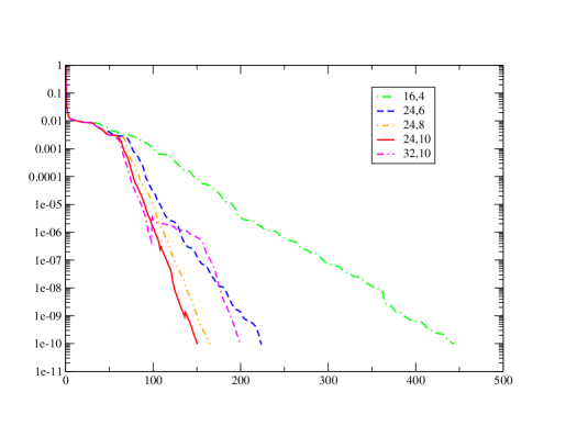
Figure 2 shows the results for flexible GMRES without deflation (left) and with deflation (right) for various choices of the cycle length . Here, as everywhere, we plot the 2-norm of the residual against the number of matrix-vector multiplications invested, i.e. for every “interior” step of the restarted GMRES cycle. In these experiments the hopping parameter was set to , which is still quite far from , so that we may consider the system as relatively well conditioned. The figures illustrate the fact that a larger value of the cycle length results in fewer iterative steps. Deflation results in fewer iterations when the cycle length is fixed. Note that the arithmetic cost related to the Arnoldi process grows like due to the orthogonalizations, so larger cycle lengths can significantly increase the computing time. This being said, Figure 2 shows that by investing just 4 vectors for deflation, we get a better performance by using a restart value than by using a restart value twice as large and no deflation.
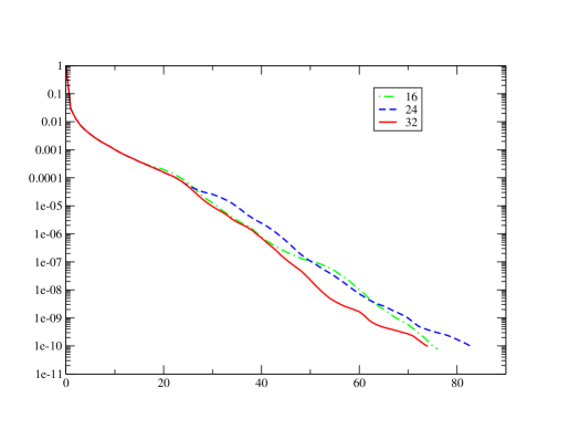
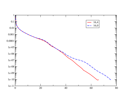
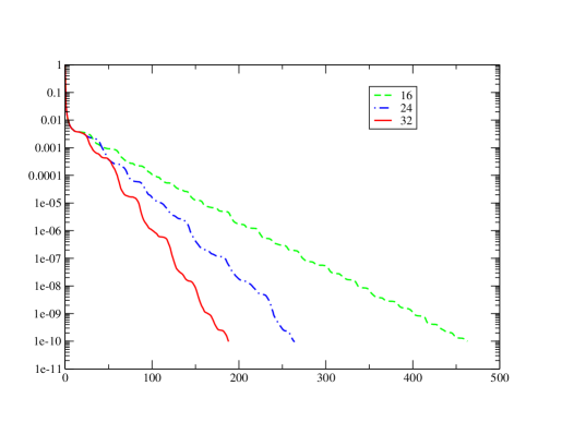
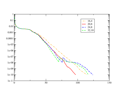
Figure 3 presents similar experiments for a different value of the hopping parameter, , which is very close to the critical value. Now the system is much more ill conditioned, and we see that deflation starts to have an even more significant impact on the performance of the method. For example, reserving vectors for deflation while using a restart value of reduces the required iterations from about to . The best deflated method uses and deflates vectors. It requires roughly only half as many iterations as the best non-deflated method which requires a much larger cycle length, . In some of the residual plots in the figure to the right we observe an increase of the residual around iterations 50-70 for some choices of the parameters. At these points we had to do a “clean” restart of FGMRES-DR, and the jump in the residual indicates the that the explicitly computed residual is considerably larger than the updated one. Since a clean restart discards all subspace information acquired so far, the subsequent GMRES cycle is comparably as slow as the very first cycle of the iteration. This shows that it might be advisable to use quite small values for the subspace dimension , since in these cases a clean restart was never necessary, thus resulting in the fastest overall convergence.
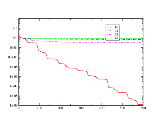
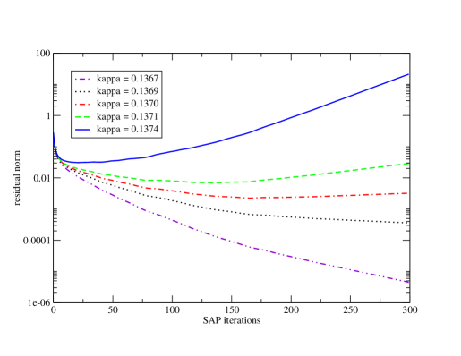
In a last experiment for this configuration we set , which is beyond the critical value. The SAP iteration by itself is divergent for this choice of (see Figure 5), and when used as a preconditioner for GMRES we observe complete stagnation unless the restart value is large enough (). On the other hand, deflation with a relatively small dimension of the deflating subspace results in quite fast convergence for moderate values of the restart value . This indicates that the divergence of the pure SAP iteration is due to the fact that just a few eigenvectors belonging to the corresponding iteration matrix are troublesome and that they are effectively removed by deflation.
The second set of experiments consists of inversions of a state-of-the-art lattice configuration thermalized at and , while
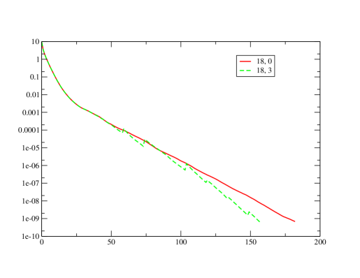
In this case a full 256 nodes QPACE rack was used. The machine is configured as a 3D torus and we used an SAP block size of that fits the 8 SPU local stores nicely and satisfies all the lattice and implementation constraints. For the test inversions presented, we have chosen to use aggressive preconditioner settings that are particularly advantageous on massively parallel machines. These settings reduce the overhead of global sums and scalar products — global sums being limited by network latency and local scalar products by memory bandwidth. In the preconditioner, we therefore performed 24 SAP cycles with 6 MR iterations for the subdomains. Figure 6 shows that for , using a small dimension for the deflating subspace, i.e., , and keeping the restart length fixed to , the iteration number decreases from 183 to 159, i.e., by about 15%. For the larger value of , deflating 3 vectors halves the iteration numbers from approximately 500 down to 250. Increasing the cycle length does not substantially affect the deflated method. Figure 7 shows results for larger values of . For non-deflated restarted GMRES almost stagnates even if we use a relatively large cycle length, . On the other hand, deflating 3 or 6 vectors cures this stagnation completely, and we can even reduce the cycle length down to 24 or even 16. A similar observation holds for .
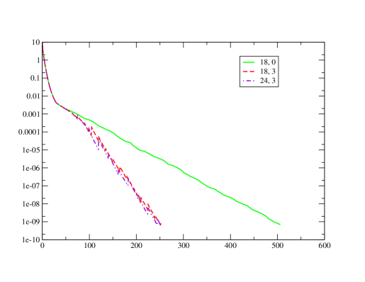
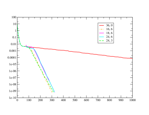
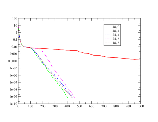
In Table 1 we report the timings on QPACE for all our computations on configurations. These numbers show that wall clock time follows the iteration counts very closely. For the range tested, the cycle length by itself has only a marginal influence. This is due to the fact that our code spends most of its time in the 24 SAP iterations of the preconditioner, so that the work for the Arnoldi process, which increases with , is relatively cheap for any of our choices for .
| kappa | m | k | iterations | time (s) |
|---|---|---|---|---|
| 0.13663 | 18 | 0 | 183 | 39.0 |
| 0.13663 | 18 | 3 | 159 | 35.9 |
| 0.13666 | 18 | 0 | 507 | 107.1 |
| 0.13666 | 18 | 3 | 255 | 56.7 |
| 0.13666 | 24 | 3 | 252 | 57.4 |
| 0.13668 | 36 | 0 | 3464 | 741.9 |
| 0.13668 | 16 | 6 | 302 | 70.4 |
| 0.13668 | 18 | 6 | 326 | 74.9 |
| 0.13668 | 24 | 6 | 325 | 73.7 |
| 0.13668 | 24 | 3 | 315 | 69.9 |
| 0.13670 | 48 | 0 | 2869 | 623.6 |
| 0.13670 | 48 | 4 | 409 | 92.3 |
| 0.13670 | 24 | 4 | 448 | 100.0 |
| 0.13670 | 24 | 6 | 461 | 106.1 |
| 0.13670 | 18 | 6 | 441 | 102.0 |
7 Conclusions
While SAP can be implemented efficiently on current supercomputers with a deep memory hierarchy and many compute cores like QPACE, it is not necessarily a convergent iteration, particularly if the hopping parameter is close to the critical value. This can very severely impede the convergence of SAP preconditioned restarted flexible GMRES or restarted GCR. We have introduced deflated restarted flexible GMRES as a (Clover) Wilson fermion solver to cure this problem. Numerical results obtained for thermalized configurations of size up to show that using a very small dimension for the deflating subspace (never more than 6) always results in satisfactory convergence speeds. An additional benefit is that deflation allows to use relatively small cycle lengths (in our experiments, to was always sufficient), which reduces the arithmetic cost of the Arnoldi process and, more importantly, keeps memory requirements low. The benefits of deflation are most prominent when the hopping parameter is close to the critical value or even larger than , so that deflation is particularly helpful on exceptional configurations arising during an HMC simulation.
The parameter space on which the performance of SAP preconditioned deflated restarted flexible GMRES can be optimized, is very large: the size and shape of the subdomains for SAP, the method and number of iterations to use for the (approximate) subdomain solves, the number of SAP iterations per preconditioning step, the cycle length and the deflating subspace dimension . We could therefore not perform a complete investigation of this parameter subspace. Rather, our approach was to fix parameters related to the SAP preconditioner by efficiency considerations for our given hardware, and then find good values for and . Although this quite surely means that we missed the overall best method, all our results consistently indicate that it is always worth to include a (small) deflating subspace: Convergence is faster for the same cycle length, and for hard problems, convergence is enabled at all. We thus think that deflated restarted flexible GMRES should establish itself as the standard successor to flexible restarted GMRES or GCR and even more to preconditioned BiCGstab for which we observed convergence problems relatively often during simulations for large configurations.
We note that an alternative approach to the method presented here are multilevel methods like adaptive algebraic multigrid, see [27, 28] or Lüschers deflated domain decomposition method [29] and its true multilevel variants [30]. As compared to these approaches, the deflated GMRES method does not require a set-up phase which can be relativley costly for the other methods if only one or a few right hand sides have to be solved. It has also the advantage of being quite simple to implement and to fit modern supercomputer architectures well.
Acknowledgements
We would like to thank Dirk Pleiter for his continuing support of this work and Tilo Wettig and Jaques Bloch for illuminating discussions. We are grateful to Xavier Pinel for making his FORTRAN code on FGMRES-DR available to us.
8 Bibliography
References
- [1] C. Gattringer, C. B. Lang, Quantum Chromodynamics on the Lattice, Springer, 2009.
- [2] S. Duane, A. Kennedy, B. Pendelton, D. Roweth, Hybrid Monte Carlo, Phys. Lett. B195 (1987) 216–222.
- [3] H. Baier, et al., QPACE: A QCD parallel computer based on Cell processors, PoS(Lattice 2009)001, arXiv: 0911.2174 [hep-lat].
- [4] H. Baier, et al., QPACE: Power-efficient parallel architecture based on IBM PowerXCell 8i, Computer Science - Research and Development 25 (2010) 149.
- [5] S. Ashby, et al., The opportunities and challenges of exascale computing, U. S. Dept. of Energy Office of Science, http://science.energy.gov/~/media/ascr/ascac/pdf/reports/Exascale_subco%mmittee_report.pdf (2010).
- [6] M. Frigo, S. G. Johnson, The design and implementation of FFTW3, Proceedings of the IEEE 93 (2005) 216––231.
- [7] K. G. Wilson, Quarks and strings on a lattice, in: A. Zichichi (Ed.), New Phenomena In Subnuclear Physics. Part A. Proceedings of the First Half of the 1975 International School of Subnuclear Physics, Erice, Sicily, July 11 - August 1, 1975, Vol. 321 of CLNS Reports, Plenum Press, New York, 1977, p. 69.
- [8] W. Hackbusch, Iterative Solution of Large Sparse Systems of Equations, Springer, 1994.
- [9] B. F. Smith, P. E. Bjørstad, W. D. Gropp, Domain Decomposition. Parallel Multilevel Methods for Elliptic Partial Differential Equations, Cambridge University Press, 1996.
- [10] M. Lüscher, Solution of the Dirac equation in lattice QCD using a domain decomposition method, Comput. Phys. Commun. 156 (2004) 209–220, arXiv:hep-lat/0310048v1.
- [11] A. Nobile, Solving the Dirac equation on QPACE, PoS(Lattice 2010)034, arXive 1109.4279 [hep-lat].
- [12] Y. Nakamura, A. Nobile, D. Pleiter, H. Simma, T. Streuer, T. Wettig, F. Winter, Lattice QCD applications on QPACE, arXiv: 1103.1363 [hep-lat].
- [13] Y. Saad, M. H. Schultz, GMRES: a generalized minimal residual algorithm for solving nonsymmetric linear systems, SIAM J. Sci. Stat. Comput. 7 (1986) 856–869.
- [14] O. Axelsson, A generalized conjugate gradient, least square method, Numer. Math. 51 (1987) 209–227.
- [15] Y. Saad, Iterative Methods for Sparse Linear Systems, 2nd edition, SIAM, Philadelpha, PA, 2003.
- [16] Y. Saad, A flexible inner-outer preconditioned GMRES algorithm, SIAM J. Sci. Stat. Comput. 14 (1993) 7461–469.
- [17] P. Jiránek, M. Rozložník, M. H. Gutknecht, How to make simpler GMRES and GCR more stable, SIAM J. Matrix Anal. Appl. 30 (4) (2008) 1483–1499.
- [18] R. B. Morgan, GMRES with deflated restarting, SIAM J. Sci. Comput. 24 (2002) 20–37.
- [19] A. Chapman, Y. Saad, Deflated and augmented Krylov subspace techniques, Numer. Linear Algebra Appl. 4 (1997) 43–66.
- [20] R. B. Morgan, A restarted GMRES method augmented with eigenvectors, SIAM J. Matrix Anal. Appl. 16 (1995) 1154–1171.
- [21] R. B. Morgan, Implicitly restarted GMRES and Arnoldi methods for nonsymmetric systems of equations, SIAM J. Matrix Anal. Appl. 21 (2000) 1112–1135.
- [22] C. Paige, B. Parlett, H. V. der Vorst, Approximate solutions and eigenvalue bounds from Krylov subspaces, Numer. Linear Algebra Appl. 2 (1995) 115–134.
- [23] X. Pinel, A perturbed two-level preconditioner for the solution of three-dimensional heterogeneous Helmholtz problems with applications to geophysics, Ph.D. thesis, Institut National Polytechnique de Toulouse, "http://www.cerfacs.fr/algor/reports/Dissertations/TH_PA_10_55.pdf" (May 2010).
- [24] L. Giraud, S. Gratton, X. Pinel, X. Vasseur, Flexible GMRES with deflated restarting, SIAM J. Sci. Comput. 32 (4) (2010) 1858–1878.
- [25] J. Demmel, Y. Hida, W. Kahan, X. S. Li, S. Mukherjee, E. J. Riedy, Error bounds from extra-precise iterative refinement, ACM Trans. Math. Softw. 32 (2006) 325–351.
- [26] B. Sheikholeslami, R. Wohlert, Improved continuum limit lattice action for QCD with Wilson fermions, Nucl. Phys. B 259 (1985) 572.
- [27] J. Brannick, R. C. Brower, M. A. Clark, J. C. Osborn, C. Rebbi, Adaptive multigrid algorithm for lattice QCD, Phys. Rev. Lett. 100:041601, arXiv:0707.4018v1 [hep-lat].
- [28] R. Babich, J. Brannick, R. C. Brower, M. A. Clark, T. A. Manteuffel, S. F. McCormick, J. C. Osborn, C. Rebbi, Adaptive multigrid algorithm for the lattice Wilson-Dirac operator, Phys. Rev. Lett. 105:201602, arXiv:1005.3043v2 [hep-lat].
- [29] M. Lüscher, Local coherence and deflation of the low quark modes in lattice QCD, JHEP 07(2007)081, arXiv:0706.2298v4 [hep-lat].
- [30] A. Frommer, K. Kahl, S. Krieg, B. Leder, M. Rottmann, Aggregation-based multilevel methods for Lattice QCD, Proceedings of Science, http://pos.sissa.it, poS(Lattice 2011)046 (2011).