A recent tipping point in the Arctic sea-ice cover: abrupt and persistent increase in the seasonal cycle since 2007

Abstract

There is ongoing debate over whether Arctic sea-ice has already passed a ‘tipping point’, or whether it will do so in the future. Several recent studies argue that the loss of summer sea ice does not involve an irreversible bifurcation, because it is highly reversible in models. However, a broader definition of a ‘tipping point’ also includes other abrupt, non-linear changes that are neither bifurcations nor necessarily irreversible. Examination of satellite data for Arctic sea-ice area reveals an abrupt increase in the amplitude of seasonal variability in 2007 that has persisted since then. We identified this abrupt transition using recently developed methods that can detect multi-modality in time-series data and sometimes forewarn of bifurcations. When removing the mean seasonal cycle (up to 2008) from the satellite data, the residual sea-ice fluctuations switch from uni-modal to multi-modal behaviour around 2007. We originally interpreted this as a bifurcation in which a new lower ice cover attractor appears in deseasonalised fluctuations and is sampled in every summer-autumn from 2007 onwards. However, this interpretation is clearly sensitive to how the seasonal cycle is removed from the raw data, and to the presence of continental land masses restricting winter-spring ice fluctuations. Furthermore, there was no robust early warning signal of critical slowing down prior to the hypothesized bifurcation. Early warning indicators do however show destabilization of the summer-autumn sea-ice cover since 2007. Thus, the bifurcation hypothesis lacks consistent support, but there was an abrupt and persistent increase in the amplitude of the seasonal cycle of Arctic sea-ice cover in 2007, which we describe as a (non-bifurcation) ‘tipping point’. Our statistical methods detect this ‘tipping point’ and its time of onset. We discuss potential geophysical mechanisms behind it, which should be the subject of further work with process-based models.

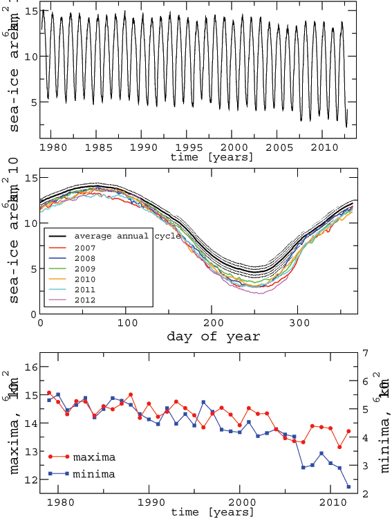
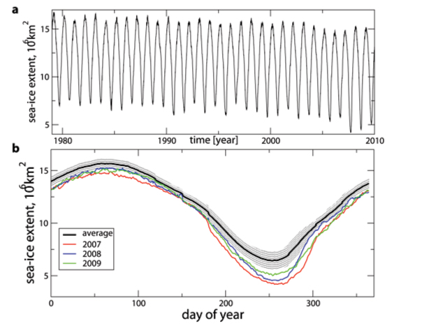
Introduction. Arctic sea-ice has experienced striking reductions in areal coverage (Stroeve et al., 2007; Nghiem et al., 2007), especially in recent summers, with 2007-2012 having the six lowest ice cover minima in the satellite record (Figure 1). Observations have fallen below IPCC model projections (Stroeve et al., 2007), despite the models having been in agreement with the observations in the 1970s. The latest models are more consistent with satellite observations (1979-present), but still fail to capture the full extent of the observed downward trend (Stroeve et al., 2012). Summer ice cover is forecast to disappear later this century (Boe et al., 2009), but the nature of the underlying transition is debated (Lenton et al., 2008; Lindsay and Zhang, 2005; Amstrup et al., 2010; Winton, 2006; Eisenman and Wettlaufer, 2009; Tietsche et al., 2011).

Arctic sea-ice has been identified as a potential tipping element in the Earth’s climate system (Lenton et al., 2008), and at least one study suggests it has already passed a ‘tipping point’ (Lindsay and Zhang, 2005). In the future, some models forecast abrupt ice loss events (Amstrup et al., 2010), on the way to a seasonally ice-free Arctic. These may qualify as passing tipping points following the broad definition given in (Lenton et al., 2008) of a point at which a small change in forcing leads to a qualitative change in the future state of a system. The definition includes both reversible and irreversible transitions, bifurcations and some non-bifurcation phenomena.

However, most recent papers on the Arctic sea-ice opt for a narrower definition of a tipping point, addressing whether summer sea-ice loss will involve an irreversible (e.g. saddle-node/fold) bifurcation. They find instead that in models the loss of summer sea-ice cover is highly reversible (Amstrup et al., 2010; Winton, 2006; Eisenman and Wettlaufer, 2009; Tietsche et al., 2011). Abrupt ice loss events are then attributed to the loss of year-round sea-ice in the Arctic making the remaining ice more vulnerable to summer melt, and prone to larger fluctuations in area coverage (Notz et al., 2009). An exception is a recent model (Abbot et al., 2011) showing that positive feedbacks involving clouds can create multiple stable states for seasonal ice cover and bifurcations between them. Furthermore, models of past abrupt climate changes in the Arctic have shown multiple stable states for sea-ice cover in the Barents and Kara Seas region and abrupt switches between them (Bengtsson et al., 2004; Semenov et al., 2009). This suggests that sub-Arctic scale ‘tipping points’ in sea-ice cover are conceivable.

On viewing the satellite-derived daily record of sea-ice area from 1979 to present (Figure 1a), it is clear that the last five years have been characterized by an increase in the amplitude of seasonal sea-ice variation (Figure 1b). The annual ice cover minimum dropped the order of $\sim$10⁶ km² more than the annual maximum in 2007 and the difference has been maintained since then (Figure 1c). This already suggests an abrupt and persistent change in sea-ice dynamics. It led us to hypothesize that the sea-ice may have passed a bifurcation-type tipping point, in which a new attractor for lower summer-autumn sea-ice cover became stable and began to be sampled in summer 2007, and in every summer since, with seasonal switches to/from the pre-existing attractor – see Figure 10 of (Livina and Lenton, 2012).

We arrived at this hypothesis by applying recently developed methods of time-series analysis that can detect changes in the modality of data (Livina et al., 2010, 2011; Cimatoribus et al., 2012) and in some cases forewarn of bifurcations (Scheffer et al., 2009; Held and Kleinen, 2004; Livina and Lenton, 2007; Lenton, 2011). Our analysis concentrates on the satellite-derived daily record of sea-ice area from 1979 to 2011 (Figure 1a), and is repeated on the shorter record of sea-ice extent 1979-2009 (Eisenman, 2010) (Figure 10) in the Appendix. For much of our analysis, a mean seasonal cycle (Figure 1b) averaged over the period 1979-2008 was removed from the data, because there is a very strong seasonally-forced variation in sea-ice area. The averaged seasonal cycle of the Arctic sea-ice 1979-2008 (Figure 1b) is very close to a sine wave (no asymmetry over seasons), and we were interested in studying the behavior of fluctuations from this typical state of seasonal variation.

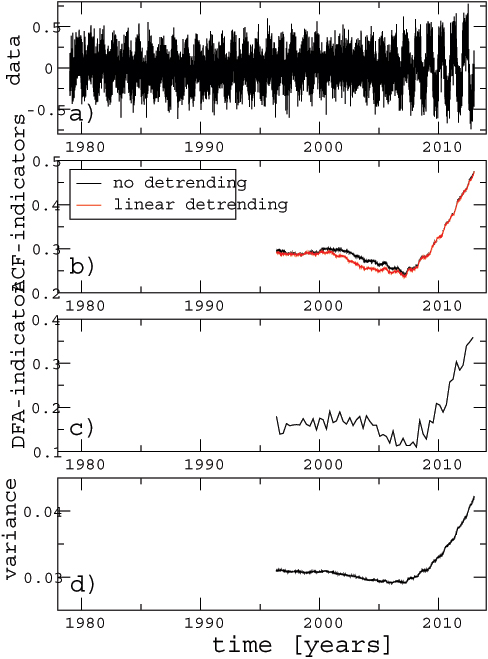
However, our interpretation in terms of a changing number of sea-ice attractors (Livina and Lenton, 2012), can be profoundly altered by changing the interval that is considered the baseline state for the sea-ice (Ditlevsen, 2012). The central problem is that any residual seasonal cycle remaining in the data appears bi-modal, and if there has been a jump in the amplitude of the seasonal cycle around 2007, it is not possible to remove one average seasonal cycle from the whole record and get rid of all the residual seasonality (Ditlevsen, 2012). We examine this further here with a stochastic model of growing amplitude in the seasonal cycle, by comparing analysis of the artificial data from this model with that of the observed data.

The paper is organized as follows: Section 2 details the data pre-processing and the methods applied. Section 3 presents the results and discusses them, including some tentative geophysical interpretation. Section 4 concludes.

1 Methodology

1.1 Data and pre-processing

Sea-ice area takes into account the fraction of a grid cell that is covered by sea ice, and can be biased low, especially in summer when melt ponds are present. Sea-ice extent assumes that any grid point with more than a certain per cent (for instance, 15%) sea ice concentration is totally covered.

Sea ice area data were obtained from ‘The Cryosphere Today’ project of the University of Illinois. This dataset uses SSM/I and SMMR series satellite products and spans 1979 to present at daily resolution. The most recent data in this series is derived from the Near-Real-Time DMSP SSM/I-SSMIS Daily Polar Gridded Sea Ice Concentrations of the National Snow & Ice Data Centre (NSIDC), see (Maslanik and Stroeve, 1999).

The sea-ice extent time series was derived by (Eisenman, 2010) (data available from ftp://ftp.agu.org/apend/gl/2010gl043741) on the basis of sea ice concentration using the NASA Team algorithm from Nimbus-7 SMMR (1978-1987), DMSP SSM/I (1987-2009), and DMSP SSMIS (2008-present) satellite passive microwave radiances on a 25km x 25km polar stereographic grid (Cavalieri et al., 1996; Meier et al., 2006; Maslanik and Stroeve, 1999). During periods of instrumental transitions, the overlapping datasets were averaged. Extent was calculated by summing the areas of all grid boxes with at least 15% ice concentration. Details of the spatial data interpolation are given by (Eisenman, 2010). The time series spans 1979-2009, and where it has 2-day resolution (when SMMR operated every other day in three months during the record, in 10/1978, 12/1987 and 1/1988), we interpolate to daily resolution to obtain a homogeneous time-series.

For both datasets – area and extent – the mean seasonal cycle over the first 30 years of data (1979-2008) was removed, as on ‘The Cryosphere Today’ website (and widely reproduced elsewhere). We also examined the effect of constructing and removing a different averaging interval (1979-2011), which produces a very similar residual series, just vertically shifted along the y-axis, i.e. the dynamics of the residual fluctuations remained the same. Hence this gives similar results and we do not show it here.

We also analyzed a derived index of ‘equivalent sea-ice extent’ (Eisenman, 2010) (available from ftp://ftp.agu.org/apend/gl/2010gl043741), which is based on the latitude of the sea-ice edge where it is free to migrate, converted to an area, assuming there were no continents present.

1.2 Potential analysis

To detect any multi-modality in the sea-ice residual data, we use a recently-developed (Livina et al., 2010, 2011) and blind-tested (Livina et al., 2011) method of ‘potential analysis’. This assumes that a system is experiencing sufficient short-term stochastic variability (noise) that it is sampling all of its available states or attractors (given a sufficiently long time window). Then we take advantage of the fact that the stationary probability distribution of the resulting data is directly related to the shape of the underlying potential, which describes the number of underlying attractors and their stability (Livina et al., 2011). Thus, with a sufficiently long time window of data one can deduce the number of attractors and their relative stability or instability.

The time series are modelled by the stochastic differential equation:

$$\dot{z}(t)=-U^{\prime}(z)+\sigma\eta,$$ (1)

where $U$ is a polynomial potential of even order, $\eta$ is a Gaussian white noise process of unit variance. Equation (1) has a corresponding Fokker-Planck equation describing the probability density function, and crucially this has a stationary solution that depends only on the underlying potential function and the noise level, $\sigma$;

$$p(z)\sim\exp\frac{-2U(z)}{\sigma^{2}}.$$ (2)

This allows the underlying potential to be reconstructed from a kernel probability distribution of time-series data (and an estimate of the noise level) as:

$$U(z)=-\frac{\sigma^{2}}{2}\log p_{d}(z),$$ (3)

where $p_{d}$ is the empirical probability density of the data.

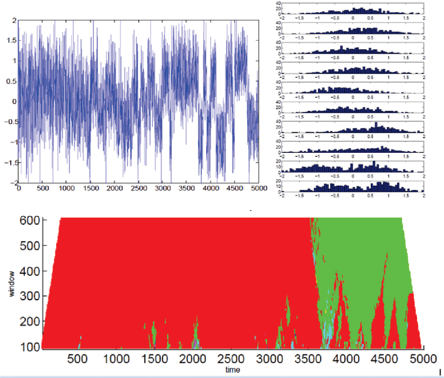
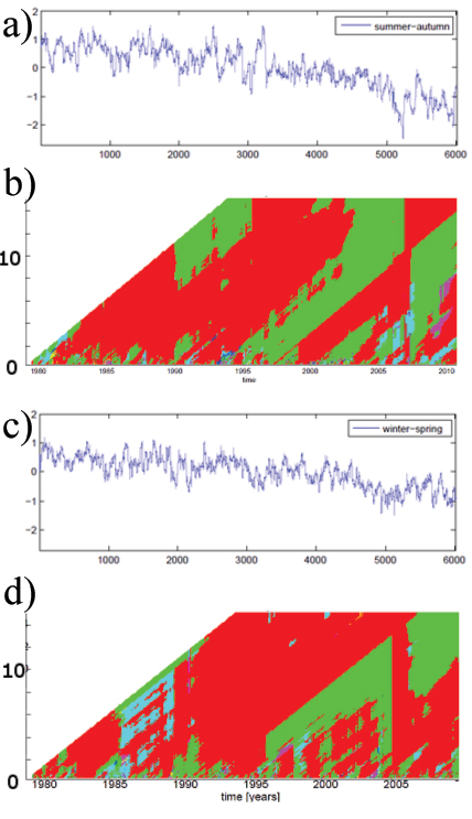
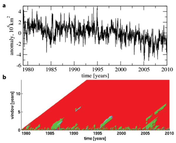
We detect the order of the polynomial and hence the number of system states following the method in (Livina et al., 2010, 2011), plotting the results as a function of window length at the end of each sliding window in a colour contour plot (e.g. Figure 3b). The rate of correct detection depends on sliding window size (Livina et al., 2011): when the window contains more than 400 data points (which in the case of daily sea-ice data corresponds to about 1.1 years), the success rate is 80%, even when noise level is up to five times bigger than the depth of the potential well; for larger windows it approaches 98%. A test of the method on artificial data, generated from a model system in which the underlying potential bifurcates from one state to two, illustrates correct detection of the number of system attractors (Figure 2).

Such tests employ Gaussian white noise, whereas sea-ice data is correlated. In the case of correlated data, the probability density under investigation is the same (a pdf aggregates data without taking into account its temporal organization). However, correlated data is more likely to sample another state due to drift (red noise) than is white noise. Hence correlated data may have better detection rate statistics than uncorrelated data.

We derive the coefficients describing the shape of the potential using an unscented Kalman filter (Livina et al., 2010, 2011), while we estimate the noise level using wavelet de-noising with Daubechies wavelets of 4th order (Livina et al., 2011).

The method assumes each subset of data is quasi-stationary and the noise is Gaussian white. For the 4-year intervals used to reconstruct the potentials in e.g. Figure 3c, the assumption of stationarity is reasonable. The noise in geophysical systems may be red rather than white, but the assumption of white noise can still be valid provided that the noise is stationary (DFA fluctuation exponent less than 1). By applying the potential model in such cases, we may attribute part of the noise variability to the potential dynamics when analysing the two components of the potential model. This model is an approximation; still it allows us to derive accurately the structure of the potential for systems with stationary red noise. When there are no non-stationarities such noise cannot artificially create an additional system state.

1.3 Critical slowing down

To test for bifurcation in the residual sea-ice fluctuations we look for the signal of ‘critical slowing down’ beforehand (Scheffer et al., 2009). Namely, for a low-order dynamical system approaching a bifurcation where its current state becomes unstable, and it transitions to some other state, one can expect to see it become more sluggish in its response to small perturbations (Scheffer et al., 2009). This can hold even for complex systems such as the sea-ice, if they exhibit a bifurcation point, because near to it their behavior will reduce down to that of a low-order system (following the Center Manifold Theorem). The signal of ‘critical slowing down’ is detectable as increasing autocorrelations in time series data, occurring over timescales capturing the decay of the major mode in the system (Held and Kleinen, 2004), which is controlled by the leading eigenvalue. We looked for this early warning indicator in the form of rising lag-1 autocorrelation (Held and Kleinen, 2004) (ACF-indicator), and through detrended fluctuation analysis (DFA-indicator) as a rising scaling exponent (Livina and Lenton, 2007). Parabolic trends were removed prior to estimating these two indicators (previously termed ‘propagators’) of critical slowing down. This is because any trend affects autocorrelations and hence may cause false positive signals in the indicators. To test robustness we also performed an alternative pre-processing of data; first removing the quadratic downward trend and then deseasonalising the data, and obtained equivalent results.

1.3.1 ACF-indicator

Lag-1 autocorrelation was estimated (Held and Kleinen, 2004; Livina and Lenton, 2007) by fitting an autoregressive model of order 1 (linear AR(1)-process) of the form:

$$z_{t+1}=c\cdot z_{t}+\sigma\eta_{t},$$ (4)

where $\eta_{t}$ is a Gaussian white noise process of unit variance, and the ‘ACF-indicator’ (AR1 coefficient):

$$c=e^{-\kappa\Delta t},$$ (5)

where $\kappa$ is the decay rate of perturbations, and $\kappa\to 0$ (i.e. $c\to 1$) as bifurcation is approached (Held and Kleinen, 2004).

1.3.2 DFA-indicator

Detrended fluctuation analysis (DFA) extracts the fluctuation function of window size $s$, which increases as a power law if the data series is long-term power-law correlated:

$$F(s)\propto s^{\alpha}$$ (6)

where $\alpha$ is the DFA scaling exponent. In the short-term regime, as $c\to 1$ of the AR(1)-model, the slowing exponential decay is well approximated by a power law in which $\alpha\to 1.5$, in the time interval 10-100 units. Exponent $\alpha$ is rescaled, following (Livina and Lenton, 2007), to give a ‘DFA-indicator’ that reaches $1$ at critical behavior.

1.3.3 Variance

We also monitored variance (calculated as standard deviation), because if a state is becoming less stable this can be characterized by its potential well getting shallower, causing increased variability over time (although this is not independent of lag-1 autocorrelation (Ditlevsen and Johnsen, 2010)).

1.3.4 Indicator trends

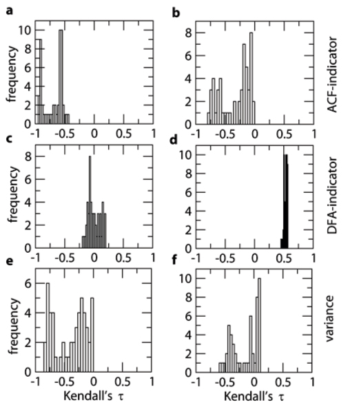
Upward trends in the indicators (rather than their absolute value) provide the primary early warning signal. The Kendall $\tau$ rank correlation coefficient (Kendall, 1948) measures the strength of the tendency of an indicator to increase (positive values) or decrease (negative values) with time, against the null hypothesis of a random sequence of measurements against time (value approximately zero). As a sensitivity analysis, the sliding window along the time series was varied from 1/4 to 3/4 of the series length.

1.4 Model of increasing seasonal cycle

To examine whether the results obtained could be explained by an increase in the amplitude of the seasonal cycle (Ditlevsen, 2012), we built a simple stochastic model, described by the following equation:

$$\begin{array}[]{c}x(t)=L+A\cdot\sin\left(\frac{2\pi t}{365}\right)+\sigma\eta,\\[10.0pt] A=\left\{\begin{array}[]{l}1,\ \ \mbox{when}\ t=1,\,\dots\,,7300,\\[10.0pt] \frac{0.5}{12410-7300}t+\frac{12410-1.5\cdot 7300}{12410-7300},\\[10.0pt] \mbox{when}\ t=7301,\,\dots\,,12410,sign\left(\sin\left(\frac{2\pi t}{365}\right)\right)<0,\end{array}\right.\end{array}$$

where $\eta$ is Gaussian white noise of unit variance, $\sigma=0.15$. This simulates sinusoidally varying ‘daily’ data (period 365) over a period $t=1:12410$ corresponding to 34 years, equivalent to period 1979-2012. A global declining trend of the data is simulated as linear in form; $L=-0.02\cdot t+55.82$. Also the amplitude of the lower half of the sine wave starts to grow linearly after 20 ‘years’ of simulated data (i.e. in ‘year’ 1998), such that it changes from -1 to -1.5 at the end of time series.

The model data was pre-processed similarly to the sea-ice data; We first deseasonalised the model data (removing 365-day ‘seasonal’ average) and performed potential analysis of the residuals. We then removed a quadratic trend from the series and calculated the early warning indicators.

2 Results and Discussion

2.1 Multi-modality detection

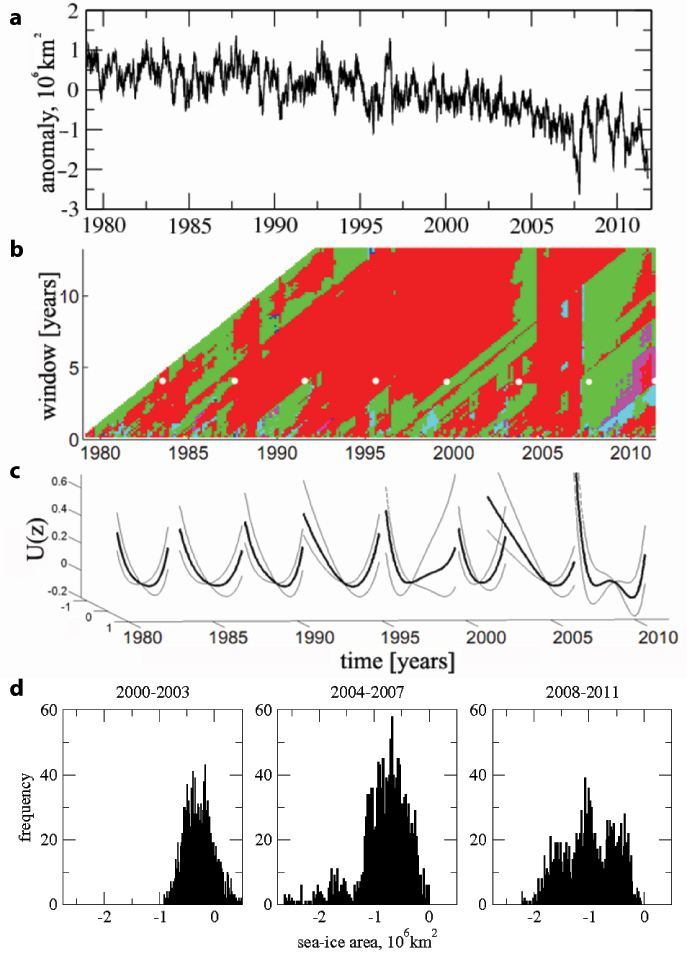
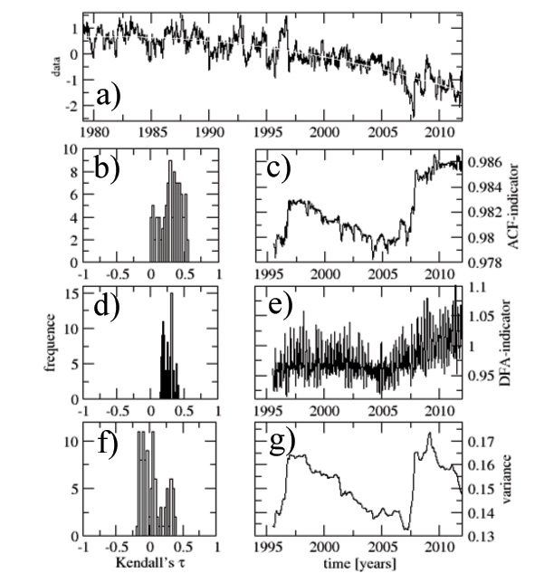
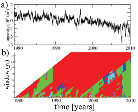
After removing the mean seasonal cycle (1979-2008), the remaining fluctuations in sea-ice area include some of order 10⁶ km² (Figure 3a). The largest anomalies are in 1996 (maximum of the series) and 2007-2011 (minima). They typically occur in the summer-autumn, when the sea-ice area is at its lowest in the seasonal cycle. Given the size of sea-ice fluctuations during 2007-2011 (Figure 3a) and the pronounced drop in sea-ice minima relative to sea-ice maxima since 2007 (Figure 1c), we considered whether the residuals exhibited an abrupt change to multi-modality in 2007.

On analyzing the residual sea-ice area fluctuations using our method of potential analysis, over long time windows (here $>$1 year), we typically find a single mode and corresponding attractor, representing the normal seasonal cycle of sea-ice variability (Figure 3b). Sometimes a second mode is detected associated with e.g., the sea-ice maximum in 1996, but these changes are not found simultaneously and persistently across a wide range of window lengths. However, from 2007 onwards, a persistent switch to two modes or attractors is detected, across a wide range of window lengths up to $>$10 years (Figure 3b). The same switch is also detected in analysis of the shorter record of sea-ice extent data (Figure 11b).

The stability of the attractor(s) for the residual sea-ice fluctuations can be reconstructed, in the form of potential curves for fixed intervals of the data (Figure 3c), with associated error estimates (on the coefficients of the polynomial function describing the potential (Livina et al., 2011)). The sea-ice residuals are typically characterized by a single mode and corresponding attractor. The interval 1996-9 (including the 1996 maximum anomaly) shows signs of a second higher ice cover attractor that is degenerate (i.e. not fully stable). In 2000-3 there is a return to a single attractor. In 2004-7, which includes the record September 2007 sea-ice retreat, a low ice-cover attractor starts to appear in the fluctuations. Then in 2008-11 the potential separates into two attractors, although the error range allows for one or the other of these to be degenerate.

The potential curves are derived from histograms of the original data (Livina et al., 2011) (Figure 3d), which confirm a second mode appearing among a long tail of negative fluctuations during 2004-2007, followed by a separation of multiple modes during 2008-2011, which the method fits as a bi-modal distribution. Thus, we originally hypothesized that the Arctic sea-ice recently passed a bifurcation point (Livina and Lenton, 2012), which created a new lower ice cover attractor for the residual deseasonalised fluctuations. Since then it has fluctuated between its normal attractor for seasonal variability and the new, lower ice cover attractor.

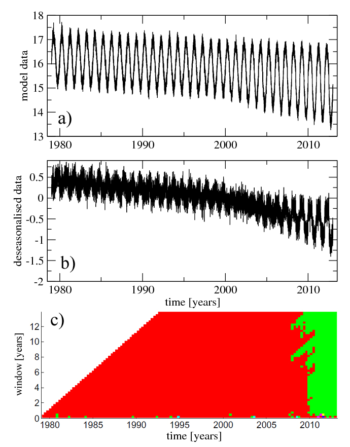
However, an abrupt change in the amplitude of the seasonal cycle will leave a residual record that has some seasonality on one side of the transition or the other (Ditlevsen, 2012). These remnant seasonal fluctuations will in turn produce a bi-modal distribution, which is accurately detected by our method – hence care is needed over how to interpret this. Sure enough analysis of the stochastic model of an increasing seasonal cycle, shows some qualitatively similar results (Fig. 4) to analysis of the real sea-ice data. In the model, imposed growth in the amplitude in the lower half of the seasonal cycle has been underway for over a decade before the residuals are detected as bi-modal. In contrast, in the real data the increase in amplitude of the seasonal cycle is abrupt (Fig. 1c) and is detected immediately (Fig. 3).

2.2 Early warnings?

Having hypothesized that a bifurcation may have occurred in Arctic sea-ice cover, we tested this by examining whether it was preceded (or followed) by any signals of destabilization in the form of critical slowing down. However, a caveat here is that the inferred bifurcation (Figures 3, 11), if correct, represents the creation of a new ice cover attractor (for the residual fluctuations) rather than the total loss of stability of the existing ice cover attractor. Hence the existing ice cover attractor may not show clear destabilization prior to the bifurcation.

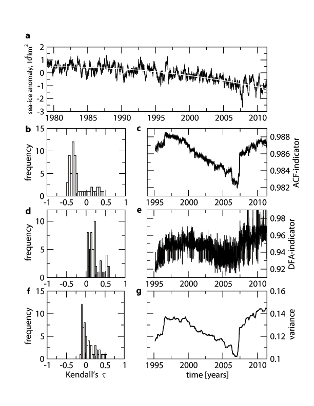
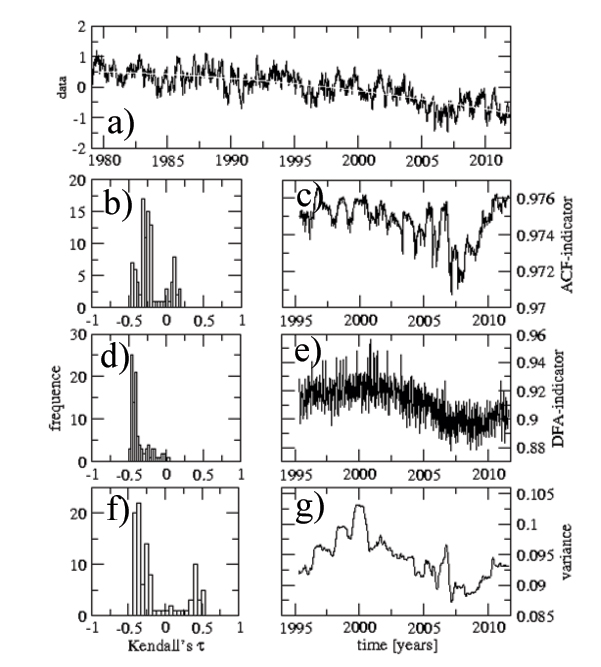
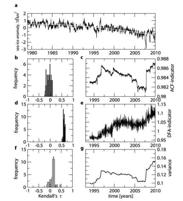
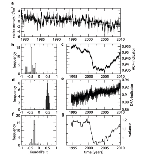
Prior to 2007 there is no consistent early warning signal of destabilization (Figure 5c,e,g). The indicators all increased around the anomalous sea-ice maximum in 1996, but then they all declined toward 2007, consistent with our potential reconstruction (Figure 3c). The only early warning signal prior to 2007 is a rise in the DFA-indicator in analysis of sea ice extent (Figure 12). Sensitivity analysis confirms this is the only robust increase across the three indicators and the two datasets, prior to 2007 (Figure 13). Thus, there was no consistent early warning signal of critical slowing down before the hypothesized bifurcation. Instead the sea-ice showed signs of increasing stability in the preceding decade, contrary to what would be expected from an approach to bifurcation.

The sea-ice retreat in 2007 caused abrupt increases in all the indicators, which have continued to rise since then (Figure 5c,e,g). Sensitivity analysis reveals a robust upward trend in the DFA-indicator across the whole dataset (Figure 5d), but no robust overall trend in the ACF-indicator or variance (Figure 5b,f). These results are reproduced in analysis of the shorter record of sea-ice extent data (Figure 12). The rise in the DFA-indicator could be consistent with the sea-ice having increasing ‘memory’ of its earlier states due to critical slowing down (Livina and Lenton, 2007). The somewhat different behavior of the ACF and DFA indicators could then be explained by the different time scales used for their calculation. The ACF-indicator, based only on lag-1 autocorrelation (here from one day to the next), may be monitoring the behavior of fast decay modes unrelated to critical slowing down. The DFA-indicator in contrast is calculated on time scales up to 100 days, which should be long enough to capture the slowest recovery mode of the sea-ice.

We conclude that overall the indicators detect a profound shift in the data in 2007, but do not forewarn of it. This does not convincingly support the bifurcation interpretation. Since 2007 an ongoing destabilization is detected.

The stochastic model of an increasing seasonal cycle shows no clear trend in the ACF or DFA indicators or the variance, followed by a steady rise in all the indicators as the residual data becomes bi-modal (Fig. 6). However, there are no abrupt increases in the ACF-indicator of critical slowing down or the variance (Fig. 6), as there are in analysis of the sea-ice data around 2007 (Fig. 5). This is consistent with the change in amplitude of the seasonal cycle being much more abrupt in the real data than in the model.

2.3 Seasonal analysis

Our results may be sensitive to the fact that land masses mute variations in winter-spring ice area (Eisenman, 2010), whereas summer-autumn area is less affected. To address this we analyzed a derived index of ‘equivalent sea-ice extent’ (Eisenman, 2010), which is based on the latitude of the sea-ice edge where it is free to migrate, converted to an area, assuming there were no continents present. Fluctuations are much larger in this index, and recent summer-autumn ice retreats no longer stand out as anomalous (Eisenman, 2010), hence no recent recent shift from uni-modal to multi-modal residuals is detected (Figure 14). However, there is still a signal of overall destabilization (Figure 15), which appears before the signal in actual sea-ice area (Figure 5). This suggests the abrupt change in the data detected in 2007 could be (at least partly) a geographic property of the shrinkage of summer-autumn ice cover away from the continents facilitating larger fluctuations (Eisenman, 2010).

To examine whether this is the case, we subdivided the original data (Figure 1a) into two composite series; summer-autumn (June-November inclusive) and winter-spring (December-May inclusive), removing the mean cycle from each, and re-running the analysis. Both subsets of the data carry part of the signal of abrupt change in 2007 (Figure 7), suggesting the change in the dynamics is not a purely summer-autumn phenomenon. The signal is clearest in summer-autumn, but does not span as wide a range of window lengths as in the full data analysis. However, the summer-autumn data does show upward trends in the ACF and DFA indicators and (less clearly) the variance (Figure 8), which are generally stronger than in the full dataset (Figure 5). In contrast, the winter-spring data shows no convincing upward trends in any of the indicators (Figure 9). Thus, the recent signal of increasing auto-correlation and variance (i.e. destabilization) is associated primarily with summer-autumn sea-ice fluctuations.

2.4 Summary and geophysical mechanisms

An abrupt and persistent change in sea-ice dynamics is detected to have occurred in 2007. This involves an extra $\sim$10⁶ km² or more sea-ice loss each summer-autumn since then. Our initial hypothesis that this abrupt increase in the amplitude of the seasonal cycle of sea-ice variability occurred through a bifurcation mechanism (Livina and Lenton, 2012), is not consistently supported. Thus, the underlying causal mechanism remains uncertain. Still, there must be some amplifying positive feedback mechanisms contributing to the abrupt increase in summer-autumn ice loss.

Statistical models such as ours cannot shed light on these underlying geophysical mechanisms. However, several positive feedbacks have been identified in recent data and are worth mentioning. Sea-ice retreat since 1979 has exposed a dark ocean surface, causing 85% of the Arctic region to receive an increase in solar heat input at the surface, with an increase of 5% per year in some regions (Perovich et al., 2007). This is warming the upper Arctic ocean and contributing to melting on the bottom of the sea-ice (Perovich et al., 2008). Sea-ice retreat is also amplifying warming of the lower atmosphere in the Arctic (Screen and Simmonds, 2010), which is shifting precipitation from snow to rainfall, and where rain lands on the remaining sea ice cover, it is encouraging melt (Screen and Simmonds, 2011). The loss of multi-year ice thins the average ice cover making it more vulnerable to further summer losses (Comiso, 2012). Finally, sea-ice loss is beginning to change atmospheric circulation patterns (Overland and Wang, 2010) (although how that feeds back to ice cover is unclear).

The abrupt increase in the seasonal cycle that we detect clearly does not involve total seasonal sea-ice loss and hence is sub-Arctic in scale. However, there may be a precedent for this; past abrupt Arctic cooling and warming events have been linked to switches between alternative states for sea-ice cover in the Barents and Kara Seas region (Bengtsson et al., 2004; Semenov et al., 2009). Such sub-Arctic-scale switches can still have significant impacts, indeed recent ice loss from the Barents and Kara Seas has been linked to cold winter extremes over Eurasia (Petoukhov and Semenov, 2010). The connection between surface temperature, sea level pressure and winds in the Arctic region, and their effect on the sea-ice cover is discussed by (Comiso, 2012).

Conclusions. We detect an abrupt and persistent increase in the amplitude of seasonal sea-ice variation in 2007. This involves an extra $\sim$10⁶ km² or more sea-ice loss each summer-autumn then and since. We originally hypothesized that this abrupt change could be explained in terms of a bifurcation in which a new lower ice cover attractor (for deseasonalised sea-ice fluctuations) appeared and began to be sampled in every summer-autumn from 2007 onwards. However, this interpretation is clearly sensitive to how the seasonal cycle is removed from the raw data, and also to the presence of continental land masses restricting winter-spring ice fluctuations. Furthermore, there was no robust early warning signal of critical slowing down, as would be expected prior to the hypothesized bifurcation. Early warning indicators do however show destabilization of the summer-autumn sea-ice cover since 2007. Overall, the bifurcation hypothesis lacks consistent support. Instead we can say that there has been an abrupt and persistent jump in the amplitude of the seasonal cycle of Arctic sea-ice cover in 2007 (Ditlevsen, 2012), but the underlying causal mechanism remains uncertain. We describe this as a (non-bifurcation) ‘tipping point’, because it involved an abrupt, qualitative change in the sea-ice dynamics, without any evidence for a large forcing perturbation, i.e. the abruptness resides in the internal dynamics of the Arctic climate system.

Our statistical methods detected this ‘tipping point’ and its time of onset suggesting they might usefully be applied to real-time analysis of diverse climatological data (albeit in this case the change retrospectively appears fairly clear in the raw data). However, statistical methods cannot shed light on geophysical mechanisms. To make progress on the underlying causal mechanisms requires process-based models. Potentially the statistical indicators of stability could be used to help re-calibrate the sensitivity of process-based models, which have generally proved unable to capture the observed abruptness of decline of the Arctic sea-ice cover.

Acknowledgements The research was supported by the NERC project ’Detecting and classifying bifurcations in the climate system’ (NE/F005474/1) and by the AXA Research Fund through a postdoctoral fellowship for V.N.L. Research was carried out on the High Performance Computing Cluster at the University of East Anglia. We thank J. Imbers Quintana and A. Lopes for discussions at the outset of this work, M. Scheffer and P. Ditlevsen for discussions over the interpretation of the results, and two anonymous reviewers for their robust critiques of the Discussion paper. The research was carried out on the High Performance Computing Cluster supported by the Research Computing Service at the University of East Anglia.

Figure 1: Arctic sea-ice area from satellite data. (a) Arctic sea-ice area, 1979-2012. (b) The mean annual cycle of the area data over 1979-2008 inclusive (solid line, shaded area denotes two error bars), together with the last five anomalous years. (c) Annual maxima (left axis) and minima (right axis) showing an abrupt increase in amplitude of the seasonal cycle in 2007.

Figure 2: Test of potential analysis on artificial data from a system bifurcating from one state to two. Here the underlying potential changes smoothly from one-well to double-well, described by the stochastic potential equation with varying potential wells (10 chunks of 500 points each), with the bifurcation occurring at time 3500 (a) artificial data generated from the changing potential function with a noise level 1; (b) histograms of 10 chunks of data, from top to bottom, corresponding to consequent subsets of the series (c) Contour plot of number of detected states, where red = 1 detected state, green = 2. Results plotted as a function of sliding window length at the middle of the window.

Figure 3: Analysis of Arctic sea-ice area. (a) Sea-ice area anomaly, daily data with mean seasonal cycle removed. (b) Contour plot of number of detected states, where red = 1 detected state, green = 2, cyan = 3, magenta = 4. Results plotted as a function of sliding window length at the end of the window. (c) Reconstructed potential curves of eight 4-year time intervals, corresponding to the white dots in (b). Here ’z’ is sea-ice area fluctuation on a shifted scale. Faint lines are potential curves derived from error estimates on the coefficients of the polynomial potential function (for details see ref. 11). In the penultimate interval 2004-2007 a second state starts to appear and in the final interval 2008-2011 there are two states of comparable stability. (d) Histograms of the data for 2000-2003, 2004-2007, 2008-2011 from which the corresponding potential curves are derived (see Methods).

Figure 4: Model ‘daily’ data with an overall decline and increase in the amplitude of the lower half of the sine wave ‘seasonal cycle’ as described in the text: (a) raw data, (b) deseasonalised data and (c) contour plot of the number of detected states in the deseasonalised data.

Figure 5: Search for early warning signals of bifurcation in Arctic sea-ice area data. (a) Sea-ice area anomaly (as in Figure 2a) showing the quadratic downward trend that is removed prior to calculating the instability indicators. Right panels show example indicators using a sliding window of length half the series, with results plotted at the end of the sliding window. Indicators from: (c) autocorrelation function (ACF), (e) detrended fluctuation analysis (DFA) and (g) variance. Left panels show histograms of the Kendall statistic for the trend in the indicators when varying the sliding window length from 1/4 to 3/4 of the series: (b) ACF-indicator, (d) DFA-indicator, (f) variance.

Figure 6: (a) Detrended deseasonalised model data (Figure 4) and its early warning indicators: (b) ACF-indicators (with and without linear detrending within sliding windows); (c) DFA-indicator; (d) variance.

Figure 7: Potential analysis of summer-autumn and winter-spring Arctic sea-ice area data. (a) Summer-autumn sea-ice area anomaly, daily data with mean cycle removed. (b) Contour plot of number of detected states. (c) Winter-spring sea-ice area anomaly, daily data with mean cycle removed. (d) Contour plot of number of detected states.

Figure 8: Search for early warning signals of bifurcation in summer-autumn Arctic sea-ice area. (a) Summer-autumn sea-ice area anomaly (as in Figure 12a) showing the quadratic downward trend that is removed prior to calculating the instability indicators. Right panels show example indicators from: (c) autocorrelation function (ACF), (e) detrended fluctuation analysis (DFA) and (g) variance, results plotted at end of a sliding window of length half the series. Left panels show histograms of the Kendall statistic for the trend in the indicators when varying the sliding window length from 1/4 to 3/4 of the series: (b) ACF-indicator, (d) DFA-indicator, (f) variance.

Figure 9: Search for early warning signals of bifurcation in winter-spring Arctic sea-ice area. (a) Winter-spring sea-ice area anomaly (as in Figure 12c) showing the quadratic downward trend that is removed prior to calculating the instability indicators. Right panels show example indicators from: (c) autocorrelation function (ACF), (e) detrended fluctuation analysis (DFA) and (g) variance, results plotted at end of a sliding window of length half the series. Left panels show histograms of the Kendall statistic for the trend in the indicators when varying the sliding window length from 1/4 to 3/4 of the series: (b) ACF-indicator, (d) DFA-indicator, (f) variance.

Figure 10: Arctic sea-ice extent from satellite data. (a) Arctic sea-ice extent from Eisenman (Eisenman, 2010) ftp://ftp.agu.org/apend/gl/2010gl043741. (b) The mean annual cycle of the extent data over 1979-2009 (solid line, shaded area denotes $2\sigma$ error bars), together with the last three anomalous years.

Figure 11: Analysis of Arctic sea-ice extent. (a) Sea-ice extent anomaly, daily data with mean seasonal cycle removed. (b) Contour plot of number of detected states, where red = 1 detected state, green = 2, cyan = 3, magenta = 4. Results plotted as a function of sliding window length at the end of the window.

Figure 12: Search for early warning signals of bifurcation in Arctic sea-ice extent data. (a) Sea-ice extent anomaly (as in Figure 2a) showing the quadratic downward trend that is removed prior to calculating the instability indicators. Right panels show example indicators from: (c) autocorrelation function (ACF), (e) detrended fluctuation analysis (DFA) and (g) variance, results plotted at end of a sliding window of length half the series. Left panels show histograms of the Kendall statistic for the trend in the indicators when varying the sliding window length from 1/4 to 3/4 of the series: (b) ACF-indicator, (d) DFA-indicator, (f) variance.

Figure 13: Destabilisation indicators calculated up to 2007. From; (a,c,e) sea-ice area anomaly, (b,d,f) sea-ice extent anomaly (both after detrending). Sensitivity analysis when varying sliding window length for Kendall trend statistic of: (a,b) ACF-indicator (c,d) DFA-indicator (e,f) variance.

Figure 14: Potential analysis of equivalent sea-ice extent index. (a) Dataset constructed by Eisenman (Eisenman, 2010) and available at: ftp://ftp.agu.org/apend/gl/2010gl043741, which is based on the latitude of the Arctic sea ice edge where the ice is free to migrate, converted to an equivalent area, assuming there were no land masses in the high northern latitudes. (b) Contour plot of number of detected states, where red = 1 detected state, green = 2, cyan = 3, magenta = 4. Results plotted as a function of sliding window length at the end of the window. No bifurcation is detected in this dataset, because it has much higher internal variability than sea ice extent (Figure 12(g)) and recent observed ice extent anomalies are dwarfed by earlier, larger fluctuations that are inferred would have occurred had the continents not got in the way of winter ice variations.

Figure 15: Search for signals of destabilisation in equivalent sea-ice extent. (a) Equivalent sea-ice extent index (as in Figure 11) showing the quadratic downward trend that is removed prior to calculating the instability indicators. Right panels show example indicators from: (c) autocorrelation function (ACF), (e) detrended fluctuation analysis (DFA) and (g) variance; results plotted at end of a sliding window of length half the series. Left panels show histograms of the Kendall statistic for the trend in the indicators when varying the sliding window length from 1/4 to 3/4 of the series: (b) ACF-indicator, (d) DFA-indicator, (f) variance.

References

- Abbot et al. (2011) Abbot, D.S., Silber, M., & Pierrehumbert, R.T., Bifurcations leading to summer Arctic sea ice loss. Journal of Geophysical Research 116, D19120 (2011).
- Amstrup et al. (2010) Amstrup, S.C. et al., Greenhouse gas mitigation can reduce sea-ice loss and increase polar bear persistence. Nature 468 (7326), 955-958 (2010).
- Bengtsson et al. (2004) Bengtsson, L., Semenov, V.A., & Johannessen, O.M., The Early Twentieth-Century Warming in the Arctic - A Possible Mechanism. Journal of Climate 17 (20), 4045-4057 (2004).
- Boe et al. (2009) Boe, J., Hall, A., & Qu, X., September sea-ice cover in the Arctic Ocean projected to vanish by 2100. Nature Geoscience 2 (5), 341-343 (2009).
- Cavalieri et al. (1996) Cavalieri, D., C. Parkinson, P. Gloerson, and H. Zwally, Sea ice concentrations from Nimbus-7 SMMR and DMSP SSM/I passive microwave data, 1978-2007, http://nsidc.org/data/nsidc-0051.html, Natl. Snow and Ice Data Cent., Boulder, Colo. (1996).
- Cimatoribus et al. (2012) Cimatoribus A., S. S. Drijfhout, V. Livina, and G. van der Schrier, Dansgaard-Oeschger events: tipping points in the climate system, Clim. Past Discuss., 8, 4269–4294 (2012).
- Comiso (2012) Comiso, J., Large decadal decline of the Arctic multiyear ice cover. Journal of Climate 25, 1176-1193 (2012).
- Ditlevsen and Johnsen (2010) Ditlevsen, P.D. & Johnsen, S.J., Tipping points: Early warning and wishful thinking. Geophysical Research Letters 37, L19703 (2010).
- Ditlevsen (2012) Ditlevsen, P.D., Interactive comment on ”A recent bifurcation in Arctic sea-ice cover” by V. N. Livina and T. M. Lenton. The Cryosphere Discussions 6, C1187-C1190 (2012).
- Eisenman (2010) Eisenman, I., Geographic muting of changes in the Arctic sea ice cover. Geophysical Research Letters 37 (16), L16501 (2010).
- Eisenman and Wettlaufer (2009) Eisenman, I. & Wettlaufer, J.S., Nonlinear threshold behavior during the loss of Arctic sea ice. Proceedings of the National Academy of Sciences USA 106 (1), 28-32 (2009).
- Held and Kleinen (2004) Held, H. and Kleinen, T., Detection of climate system bifurcations by degenerate fingerprinting. Geophysical Research Letters 31, L23207 (2004). ur
- Kendall (1948) Kendall, M.G., Rank Correlation Methods. (Charles Griffin & Company Limited, London, 1948).
- Kinnard et al. (2011) Kinnard, C. et al., Reconstructed changes in Arctic sea ice over the past 1,450 years. Nature 479 (7374), 509-512 (2011).
- Lenton (2011) Lenton, T.M., Early warning of climate tipping points. Nature Climate Change 1, 201-209 (2011).
- Lenton et al. (2008) Lenton, T.M. et al., Tipping Elements in the Earth’s Climate System. Proceedings of the National Academy of Sciences USA 105 (6), 1786-1793 (2008).
- Lindsay and Zhang (2005) Lindsay, R.W. & Zhang, J., The Thinning of Arctic Sea Ice, 1988-2003: Have We Passed a Tipping Point? Journal of Climate 18, 4879-4894 (2005).
- Livina et al. (2011) Livina, V.N., Ditlevsen, P.D., & Lenton, T.M., An independent test of methods of detecting and anticipating bifurcations in time-series data. Physica A: Statistical Mechanics and its Applications, doi:10.1016/j.physa.2011.1008.1025 (2011).
- Livina et al. (2010) Livina, V.N., Kwasniok, F., & Lenton, T.M., Potential analysis reveals changing number of climate states during the last 60 kyr. Climate of the Past 6 (1), 77-82 (2010).
- Livina et al. (2011) Livina, V.N., Kwasniok, F., Lohmann, G., Kantelhardt, J.W., & Lenton, T.M., Changing climate states and stability: from Pliocene to present. Climate Dynamics 37 (11-12), 2437-2453 (2011).
- Livina and Lenton (2007) Livina, V.N. & Lenton, T.M., A modified method for detecting incipient bifurcations in a dynamical system. Geophysical Research Letters 34, L03712 (2007).
- Livina and Lenton (2012) Livina V. N. and T. M. Lenton, A recent bifurcation in Arctic sea-ice cover, Cryosphere Discuss. 6, 2621–2651 (2012); doi:10.5194/tcd-6-2621-2012.
- Maslanik and Stroeve (1999) Maslanik, J., and J. Stroeve, Near real-time DMSP SSM/I daily polar gridded sea ice concentrations, http://nsidc.org/data/nsidc-0081.html, Natl. Snow and Ice Data Cent., Boulder, Colo. (1999).
- Meier et al. (2006) Meier, W., F. Fetterer, K. Knowles, M. Savoie, and M. J. Brodzik, Sea ice concentrations from Nimbus-7 SMMR and DMSP SSM/I passive microwave data, January December 2008, http://nsidc.org/data/ nsidc-0051.html, Natl. Snow and Ice Data Cent., Boulder, Colo. (2006).
- Nghiem et al. (2007) Nghiem, S.V. et al., Rapid reduction of Arctic perennial sea ice. Geophysical Research Letters 34, L19504 (2007).
- Notz et al. (2009) Notz, D., The future of ice sheets and sea ice: Between reversible retreat and unstoppable loss. Proceedings of the National Academy of Sciences USA 106, 20590-20595 (2009).
- Overland and Wang (2010) Overland, J.E. & Wang, M., Large-scale atmospheric circulation changes are associated with the recent loss of Arctic sea ice. Tellus A 62 (1), 1-9 (2010).
- Perovich et al. (2007) Perovich, D.K. et al., Increasing solar heating of the Arctic Ocean and adjacent seas, 1979-2005: Attribution and role in the ice-albedo feedback. Geophysical Research Letters 34, L19505 (2007).
- Perovich et al. (2008) Perovich D.K., J. A. Richter-Menge, K. F. Jones, and B.Light, Sunlight, water, and ice: Extreme Arctic sea ice melt during the summer of 2007. Geophysical Research Letters 35, L11501 (2008).
- Petoukhov and Semenov (2010) Petoukhov, V. & Semenov, V.A., A link between reduced Barents-Kara sea ice and cold winter extremes over northern continents. J. Geophys. Res. 115 (D21), D21111 (2010).
- Scheffer et al. (2009) Scheffer, M. et al., Early warning signals for critical transitions. Nature 461, 53-59 (2009).
- Screen and Simmonds (2010) Screen, J.A. & Simmonds, I., The central role of diminishing sea ice in recent Arctic temperature amplification. Nature 464 (7293), 1334-1337 (2010).
- Screen and Simmonds (2011) Screen, J. & Simmonds, I., Declining summer snowfall in the Arctic: causes, impacts and feedbacks. Climate Dynamics, 10.1007/s00382-00011-01105-00382 (2011).
- Semenov et al. (2009) Semenov, V.A., Park, W., & Latif, M., Barents Sea inflow shutdown: A new mechanism for rapid climate changes. Geophysical Research Letters 36 (14), L14709 (2009).
- Stroeve et al. (2007) Stroeve, J., Holland, M.M., Meier, W., Scambos, T., & Serreze, M., Arctic sea ice decline: Faster than forecast. Geophysical Research Letters 34, L09501 (2007).
- Stroeve et al. (2012) Stroeve J. C., V. Kattsov, A. Barrett, M. Serreze, T. Pavlova, M. Holland, W. N. Meier, Trends in Arctic sea ice extent from CMIP5, CMIP3 and observations Geophys. Res. Lett. 39, L16502 (2012), doi:10.1029/2012GL052676
- Tietsche et al. (2011) Tietsche, S., Notz, D., Jungclaus, J.H., & Marotzke, J., Recovery mechanisms of Arctic summer sea ice. Geophysical Research Letters 38 (2), L02707 (2011).
- Winton (2006) Winton, M., Does the Arctic sea ice have a tipping point? Geophysical Research Letters 33 (23), L23504 (2006).