Models of cuspy triaxial stellar systems. I. Stability and chaoticity

Abstract

We used the N–body code of Hernquist & Ostriker (1992) to build a dozen cuspy ($\gamma\simeq 1$) triaxial models of stellar systems through dissipationless collapses of initially spherical distributions of $10^{6}$ particles. We chose four sets of initial conditions that resulted in models morphologically resembling E2, E3, E4 and E5 galaxies, respectively. Within each set, three different seed numbers were selected for the random number generator used to create the initial conditions, so that the three models of each set are statistically equivalent. We checked the stability of our models using the values of their central densities and of their moments of inertia, which turned out to be very constant indeed. The changes of those values were all less than 3 per cent over one Hubble time and, moreover, we show that the most likely cause of those changes are relaxation effects in the numerical code. We computed the six Lyapunov exponents of nearly 5,000 orbits in each model in order to recognize regular, partially and fully chaotic orbits. All the models turned out to be highly chaotic, with less than 25 per cent of their orbits being regular. We conclude that it is quite possible to obtain cuspy triaxial stellar models that contain large fractions of chaotic orbits and are highly stable. The difficulty to build such models with the method of Schwarzschild (1979) should be attributed to the method itself and not to physical causes.

1 Introduction

Self-consistent models of spherical and disklike stellar systems are relatively simple to build using standard textbook methods (Binney & Tremaine, 2008), but special techniques are necessary to obtain triaxial models adequate to represent elliptical galaxies. One of the most popular of those techniques is due to Schwarzschild (1979): one chooses a reasonable mass distribution for the system, obtains the corresponding potential and computes a large library of orbits in that potential selecting suitable initial conditions; weights are then assigned, according to the time spent on each orbit and in every region of space, and used to set up a system of linear equations linking the mass density in each region to the fractions of the different types of orbits, which can be finally obtained solving the system. A different method, which we will refer to as the N–body method, was due to Sparke & Sellwood (1987): adopting an initial distribution of mass points, one integrates their equations of motion with an N–body code until an equilibrium configuration is reached; the potential is then fixed and fitted with an adequate smooth approximation that allows the computation of orbits using the positions and velocities of the bodies as initial conditions. The initial distribution of bodies can be chosen in different ways to obtain a triaxial system: slow deformation of a spherical system (Holley–Bockelmann et al., 2001), cold collapse of a spherical system (Voglis, Kalapotharakos & Stavropoulos, Voglis et al.2002, Muzzio et al.2005), merging of stellar systems (Jesseit, Naab & Burkert, 2005), and so on. Nevertheless, with the N–body method it is not possible to have the degree of control over the final configuration that one has with Schwarzschild’s method. In the end, both methods yield the same result (i.e., a self-consistent stellar system and an analysis of its orbital content), but the method of Schwarzschild (1979) starts with a chosen mass distribution, obtains orbits and finds which fractions of those orbits are needed to have a self-consistent system with that mass distribution, while the N–body method begins obtaining a self-consistent system and then performs the orbital analysis.

Chaotic motions are frequent in stellar systems (Contopoulos, 2004), and Schwarzschild (1993) realized that triaxial systems should include chaotic orbits but, when he introduced them in his models, the models evolved on time scales of the order of a Hubble time and were not truly stable. This problem was aggravated after it became clear that cuspy models (where near the centre the density, $\rho(r)$, is proportional to $r^{-\gamma}$, where $r$ is the radius and $1\leq\gamma\leq 2$) were needed for elliptical galaxies (Merritt & Fridman, 1996). Nevertheless, it is perfectly possible to obtain stable triaxial models, even cuspy ones, that contain large fractions of chaotic orbits using the N–body method (Voglis et al.2002; Muzzio et al.2005; Aquilano et al. 2007; Muzzio, Navone & Zorzi Muzzio et al.2009), so that several of those authors argued that the difficulty to build such systems with the method of Schwarzschild (1979) was due to that method itself and not to a physical cause.

Clearly, chaotic orbits are difficult to deal with when using the method of Schwarzschild (1993) because they cover different regions at different times. Worse still, in cuspy triaxial potentials chaotic orbits tend to be extremely sticky (Siopis & Kandrup, 2000), and sticky orbits behave like regular orbits for long periods of time and chaotically at other intervals. Let us assume, as an example, that chaotic orbits occupy part of the time an elongated region of space and another part of the time a nearly spherical region. Therefore, the orbits that occupy mostly an elongated region during the integration time used to prepare the library of orbits will have large weights in that region and low weights outside it; conversely, the orbits that occupy mostly the nearly spherical region during the same integration time will have a more or less even distribution of weight values over this region. Now, when these weights are used to establish the fractions of orbits that make up the triaxial system, the orbits of the former group will be strongly favoured and the equilibrium system yielded by the method of Schwarzschild (1979) will include many of them and few of the other group. If we then let the system evolve, the former orbits will tend to fill in a more spherical region as time goes by and, conversely, the latter orbits will adopt a flatter distribution. But, since the model included less orbits that originally had a more spherical distribution, the model will become rounder, as shown by the Table 6 of Schwarzschild (1993) for most of his models. The use of longer integration times, as Capuzzo–Dolcetta et al. (2007) advocated, does not guarantee the success of the method either, because the average behaviour of a chaotic orbit over a certain interval, no matter how long, does not necessarily coincide with its behaviour over a different interval, or even a subinterval, of the integration time. To make matters worse, the number of orbits typically computed for Schwarzschild’s method is not very large, from several hundreds in the works of Schwarzschild himself up to about $10,000$ in more recent work like that of Capuzzo–Dolcetta et al. (2007), so that they do not provide a strong enough statistical basis.

On the other hand, the N–body method uses large numbers of bodies (of the order of $10^{6}$ in our own more recent works) guaranteeing good statistics and the model is created by the evolution of the system itself, that is, the dynamics take care of favoring certain orbits at the expense of others so as to reach a self-consistent state. Is that state a stable one? If all the orbits are regular it certainly is because, once reached that state, the orbits will continue filling in the same regions of space for ever, in other words, we will have a static equilibrium. If the model includes chaotic orbits, however, it is conceivable that, once in equilibrium, when part of the chaotic orbits evolves to occupy a rounder space region, another part of the chaotic orbits which had a rounder distribution evolves towards a more elongated one and fill in the phase space regions left vacant by the former, that is, we might have a dynamic rather than static equilibrium. While all this is concievable there is no guarantee that it will actually happen, but the past investigations that resulted in stable models that contained high fractions of chaotic orbits undoubtedly support this view.

Therefore, we want to investigate whether it is possible to obtain self-consistent models of cuspy triaxial sytems that are stable. That is, we will deal with the type of model that is most likely to contain high fractions of chaotic orbits and most difficult to obtain with Schwarzschild’s method. We have already obtained such models with the N–body method (, Muzzio et al.2009) but, in order to compensate for the softening needed by the N–body code of L.A. Aguilar (White, 1983; Aguilar & Merritt, 1990) we had to introduce an additional potential. Here we will use the code of L. Hernquist (Hernquist & Ostriker, 1992) that does not need softening and that uses an expansion of the potential based on the model of Hernquist (1990) that is particularly adequate for cuspy models.

The next section gives a description of how we obtained our models and their main properties. Section 3 presents our results on the stability and chaoticity of the models and Section 4 summarizes our conclusions.

2 Models of cuspy triaxial stellar systems

2.1 Model building

We built our models following the recipe of Aguilar & Merritt (1990), just as we have done in our previous investigations (see , Muzzio et al.2005; Aquilano et al., 2007; , Muzzio et al.2009, for example): we randomly created a spherical distribution of $10^{6}$ particles with a density distribution inversely proportional to the distance to the centre and a Gaussian velocity distribution, and we let it collapse following the evolution with the code of Hernquist & Ostriker (1992); due to the radial orbit instability, the result is a triaxial system. The gravitational constant, $G$, the radius of the sphere and the total mass are all set equal to $1$ and the collapse time (the one needed to reach the maximum potential energy) turns out to be also very close to unity. We followed the initial collapse for 7 time units (t.u., hereafter) and, then, we eliminated the particles with positive energy, we determined the principal axes of the inertia tensor of the $80$ per cent most tightly bound particles and we rotated the system so that its major, intermediate and minor axes coincide, respectively, with the x, y and z axes of coordinates. Subsequently, we let the system evolve for another 300 crossing times ($T_{cr}$, hereafter, see Table 1 below), eliminated the less bound particles that had not yet reached equilibrium (less than $2$ or $3$ per cent of the particles in all cases) and aligned it again with the system of coordinates. We then performed a last run of $600$ $T_{cr}$ to, first, obtain the final model after the initial $100$ $T_{cr}$ and, second, check its stability over the final $500$ $T_{cr}$. We must recall that we are only interested in obtaining models morphologically similar to elliptical galaxies and not in creating them through a realistic process. Besides, we want to make sure that our models have reached the equilibrium state before testing them for possible evolutionary effects. As we will show later, one Hubble time is of the order of $200$ $T_{cr}$ for our models, so that the integration times used here are indeed much larger than that time and, as indicated, do not correspond to a realistic process of galaxy formation.

After several trials, we chose an integration step of $0.0025T_{cr}$ which yielded integration errors in the energies of the individual bodies negligibly small compared to the changes in those energies due to the relaxation effects of the code (Hernquist & Barnes, 1990). With that choice, the total energy is conserved within about $0.1$ per cent during most of the evolutions, except during the initial collapse when it is conserved only within about $1$ or $2$ per cent.

Kalapotharakos, Efthymiopoulos & Voglis (Kalapotharakos et al.2008) investigated the approximation of N–body realizations of models of Dehnen (1993) for $0\leq\gamma\leq 1$ with a generalization of the method of Hernquist & Ostriker (1992) and they found that the choice of the radial basis functions seriously affects the results of the fractions of chaotic orbits or the distribution of the Lyapunov characteristic exponents. The model of Hernquist (1990) corresponds to the $\gamma=1$ case of the models of Dehnen (1993) so that the method of Hernquist & Ostriker (1992), based on the former, should be expected to yield good results for models with $\gamma=1$ and, in fact, that is one conclusion of the work of (Kalapotharakos et al.2008). Therefore, it is important that we stick to models with $\gamma=1$, not only because they are fairly cuspy, but also because the N–body method we are using works best for such models. Notice that even our initial distribution (an sphere with density proportional to the inverse of the radius) obeys that $\gamma$ value.

The code of Hernquist & Ostriker (1992) allows one to choose the number of terms in the angular and radial expansions ($l_{max}$ and $n_{max}$, respectively), so that we performed tests with different numbers of terms in the ranges $2\leq l_{max}\leq 6$ and $4\leq n_{max}\leq 10$ (Zorzi & Muzzio, 2009). For every ($l_{max}$, $n_{max}$) pair we run three simulations that differed only in the seed number used to randomly generate the initial positions and velocities, i.e., the three were statistically equivalent. The pairs $(3,6)$, $(3.8)$, $(3,10)$, $(4,7)$, $(4,10)$, $(5,8)$ and $(6,8)$ yielded models that were only moderately cuspy, with $\gamma\simeq 0.6-0.9$, so that they were discarded. It might seem odd that, despite the use of a basis of radial functions derived from the Hernquist model, which has $\gamma=1$, the obtention of collapse models with such cuspiness is not guaranteed but, although the zero order radial function is cuspy with $\gamma=1$, higher order terms are not and in all likelihood their contribution flattens the cusp. Most of the remaining ($l_{max}$, $n_{max}$) pairs might have been acceptable, as the reasons to prefer one to another were not as compelling as the low $\gamma$ values that made us reject those mentioned before. Pairs $(2,8)$ and $(4,5)$ yielded $\gamma$ values that departed moderately (less than 0.1) from $1$, and the results from their different statistical realizations exhibited larger dispersions than other pairs. Of the three last pairs, all with $l_{max}=4$, the one with $n_{max}=6$ showed the most consistent results among the different statistical realizations, so that we finally decided to use those numbers of terms in our expansions.

2.2 The models

Following Aguilar & Merritt (1990) we took the square roots of the mean square values of coordinates of the $80$ per cent most tightly bound particles as the semiaxes of the system; the major, intermediate and minor axes will be dubbed $a$, $b$ and $c$, respectively, hereafter. We built several models adopting different values of the dispersion for the velocity distribution, obtaining less elongated models for larger dispersion values. Finally, we adopted four dispersion values that resulted in models with $c/a$ values close to $0.8$, $0.7$, $0.6$ and $0.5$, respectively (i.e., corresponding to elliptical galaxies between Hubble types E2 and E5). The velocity dispersion for the E5 model was essentially zero, so that more elongated models could not be obtained. A similar result had been obtained in our previous work (Aquilano et al., 2007), where we could not obtain models more flattened than E6 and we suggested that this might hint that mergers, rather than collapses, are needed to obtain the most elongated ellipticals. For each selected value of the velocity dispersion, three different models (dubbed $a$, $b$ and $c$) were obtained using three different seed numbers for the random number generator when creating the initial distribution of particles. In brief, we prepared a grand total of 12 models, divided in 4 groups; the models in each group resemble E2, E3, E4 and E5 galaxies, respectively, and the three models within each group differ from each other only from a microscopic point of view, being essentially identical from the point of view of their macroscopic properties. As in our previous work (Muzzio, 2006; Aquilano et al., 2007; , Muzzio et al.2009), several models display figure rotation around the minor axis, i.e., they rotate very slowly even though their total angular momentum is zero.

Table 1: Properties of our models.

$Model$	$Mass$	$T_{cr}$	$R_{e}$	$\sigma_{0}$	$T$	$\gamma$	$\omega$
E2a	0.990	0.721	0.250	0.894	0.73	1.052 $\pm$ 0.021	0.0003 $\pm$ 0.0001
E2b	0.990	0.723	0.253	0.897	0.78	0.997 $\pm$ 0.021	0.0012 $\pm$ 0.0004
E2c	0.990	0.721	0.250	0.902	0.70	1.006 $\pm$ 0.021	0.0016 $\pm$ 0.0004
E3a	0.979	0.659	0.220	0.934	0.65	1.056 $\pm$ 0.021	-0.0004 $\pm$ 0.0001
E3b	0.979	0.659	0.221	0.933	0.68	1.062 $\pm$ 0.021	0.0002 $\pm$ 0.0001
E3c	0.978	0.657	0.219	0.929	0.66	0.987 $\pm$ 0.021	0.0010 $\pm$ 0.0001
E4a	0.911	0.526	0.182	0.957	0.62	1.053 $\pm$ 0.019	0.0001 $\pm$ 0.0003
E4b	0.905	0.518	0.180	0.974	0.63	1.027 $\pm$ 0.021	-0.0002 $\pm$ 0.0001
E4c	0.908	0.521	0.180	0.963	0.62	1.073 $\pm$ 0.022	-0.0002 $\pm$ 0.0002
E5a	0.906	0.463	0.159	0.997	0.46	0.985 $\pm$ 0.022	0.0020 $\pm$ 0.0007
E5b	0.908	0.466	0.160	0.986	0.48	1.000 $\pm$ 0.019	0.0059 $\pm$ 0.0004
E5c	0.907	0.465	0.158	0.970	0.46	1.017 $\pm$ 0.020	0.0164 $\pm$ 0.0003

Table 1 summarizes the global properties of our models: mass, crossing time, effective radius, central radial velocity dispersion, triaxiality, $\gamma$ and angular velocity of figure rotation. The effective radius was obtained from the $(x,z)$ projection and, accordingly, the central radial velocity dispersion was computed from the y components of the velocities of the $10,000$ particles closer to the centre on that projection. Triaxiality was evaluated from the semiaxes obtained from the $80$ per cent most tightly bound particles as $T=(a^{2}-b^{2})/(a^{2}-c^{2})$. $\gamma$ was obtained as the slope of the $log\rho(r)$ vs. $log(r)$ line for the innermost $10,000$ particles binned in $100$ particle bins. The angular velocity was computed from the angles formed by the major axis with its original position at different times of the final $500$ $T_{cr}$ integration. The Table clearly shows that, for a given model, the different realizations obtained changing the seed number in the random number generator have essentially the same global properties. The only exception is the angular velocity which displays significant differences, particularly among models E5a, b and c. Nevertheless, rotation is very slow in all cases and, except for the E5c case, lower than the 0.00975 value of the investigation by Muzzio (2006), which revealed only very small differences between the fractions of chaotic orbits in the rotating and non-rotating system. The present E4 and E5 models are much more triaxial than the corresponding non-cuspy models of Aquilano et al. (2007) ($0.98$ and $0.81$, respectively), and the present model E4 is much more triaxial than the cuspy model E4c of (Muzzio et al.2009) ($0.91$).

As in our previous work (see Aquilano et al., 2007; , Muzzio et al.2009, for example), we chose galaxies NGC1379 and NGC4697 (Napolitano et al., 2005; Forbes & Ponman, 1999), whose mass-to-light ratio gradients are zero, to obtain some estimate of the equivalence between our units and those of real galaxies, Comparing their observed values of $R_{e}$ ($2.5$ and $5.7kpc$, respectively) and $\sigma_{0}$ ($128$ and $180\>kms^{-1}$, respectively) with those from our Table 1, we conclude that values between about $10$ and $36kpc$ can be used as our length unit and values between about $0.07$ and $0.20Gy$ as our time unit. Then, the Hubble time can be estimated as between $66$ and $190\>t.u.$, and we will adopt a value of $100\>t.u.$, hereafter.

Table 2: Major semiaxes and axial ratios of our models

$Model$	$Property$	$20\%$	$40\%$	$60\%$	$80\%$	$100\%$
	a	0.068	0.117	0.172	0.300	0.578
E2a	b/a	0.754	0.789	0.837	0.877	0.930
	c/a	0.596	0.684	0.768	0.826	0.909
	a	0.068	0.118	0.175	0.297	0.574
E2b	b/a	0.742	0.777	0.820	0.870	0.925
	c/a	0.602	0.687	0.763	0.829	0.906
	a	0.067	0.116	0.173	0.294	0.578
E2c	b/a	0.767	0.801	0.845	0.882	0.937
	c/a	0.605	0.691	0.769	0.826	0.913
	a	0.062	0.115	0.164	0.294	1.097
E3a	b/a	0.753	0.723	0.781	0.814	0.852
	c/a	0.597	0.564	0.642	0.694	0.810
	a	0.065	0.117	0.165	0.294	1.139
E3b	b/a	0.710	0.701	0.761	0.802	0.840
	c/a	0.554	0.555	0.634	0.692	0.803
	a	0.065	0.115	0.165	0.294	1.144
E3c	b/a	0.714	0.715	0.776	0.808	0.852
	c/a	0.559	0.559	0.635	0.689	0.807
	a	0.056	0.104	0.152	0.233	1.146
E4a	b/a	0.731	0.697	0.735	0.769	0.775
	c/a	0.581	0.516	0.546	0.581	0.674
	a	0.056	0.102	0.150	0.231	1.160
E4b	b/a	0.728	0.698	0.733	0.764	0.792
	c/a	0.575	0.517	0.549	0.583	0.706
	a	0.055	0.103	0.152	0.232	1.180
E4c	b/a	0.749	0.706	0.737	0.765	0.797
	c/a	0.588	0.515	0.539	0.575	0.708
	a	0.052	0.095	0.148	0.216	0.482
E5a	b/a	0.824	0.809	0.815	0.814	0.893
	c/a	0.557	0.508	0.504	0.515	0.563
	a	0.051	0.095	0.147	0.222	0.479
E5b	b/a	0.846	0.810	0.802	0.803	0.879
	c/a	0.596	0.509	0.506	0.508	0.555
	a	0.051	0.094	0.145	0.222	0.496
E5c	b/a	0.847	0.825	0.810	0.810	0.883
	c/a	0.583	0.512	0.500	0.506	0.569

We obtained the projected distributions of the particles on the $(xz)$ plane and, following Aguilar & Merritt (1990), we adopted fixed axial ratios equal to those of the $80$ per cent most tightly bound particles for each model (see below), and computed the surface density of particles in elliptical shells containing $10,000$ particles per bin. Just as Aguilar & Merritt (1990) had found for their models, ours follow very closely a de Vaucouleurs law and, again, differences among the different random realization of the same model are negligibly small. As an example, Figure 1 shows the results for our models E5.

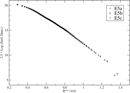
Figure 1: Surface density versus $R^{1/4}$ plot for the E5 models

Figure 2 shows, as an example, the logarithm of the density versus the logarithm of the radius for the central part of the E5 models; different symbols correspond to models with different seed numbers and a straight line with slope $\gamma=1$ is also shown for comparison. In this case the density was computed in spherical shells containing 100 particles each, so that the Poisson relative error of each point on the graph is about $0.043$. Besides, Figure 3 presents, for the innermost region of model E5c, the logarithm of the density versus the logarithm of the radius for both the adopted model (circles) as for that same model evolved $100\>t.u.$, or about a Hubble time, (plus signs) and we note that the slope of the central cusp is very well conserved. Similar results were obtained for the other models.

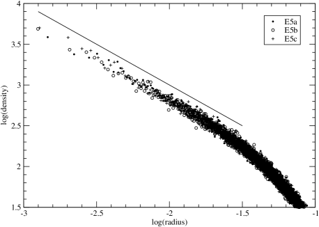
Figure 2: Density versus radius plot for the E5 models

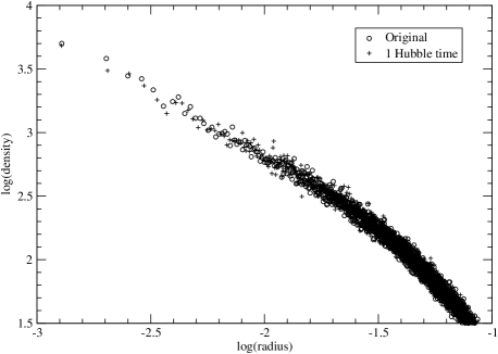
Figure 3: Density versus radius plot for the E5c model at different times.

Table 2 gives for each model the values of the major semiaxis and of the axial ratios for the $20$, $40$, …and $100$ per cent most tightly bound particles. Again, the results obtained changing the randomly generated inital conditions for a given model are essentially the same. As in our previous models, there is a general trend towards larger axial ratios at larger distances from the centre, but the trend is weaker for the more flatened models and breaks closer to the centre, probably due to the influence of the cusp.

3 Results and analysis

3.1 Stability

We used the results of the $500$ $T_{cr}$ long final evolution to check the stability of the central density and the semiaxes of the stellar systems. For this purpose, we computed at $100$ $T_{cr}$ intervals the central density from the $10,000$ particles closer to the centre of each system, and the moments of inertia of the $80$ per cent most tightly bound particles. These quantities changed almost linearly with time, so that we obtained their variations over a Hubble time from the corresponding best fitting straight lines and the results are presented in Table 3.

Table 3: Percentage variations over one Hubble time.

$Model$	$Dens.(\%)$	$Xmom.in.(\%)$	$Ymom.in.(\%)$	$Zmom.in.(\%)$
E2a	-0.61 $\pm$ 0.29	-0.63 $\pm$ 0.09	0.64 $\pm$ 0.13	0.20 $\pm$ 0.09
E2b	-0.36 $\pm$ 0.43	-0.48 $\pm$ 0.07	0.51 $\pm$ 0.08	0.41 $\pm$ 0.11
E2c	-0.83 $\pm$ 0.59	-0.45 $\pm$ 0.10	0.49 $\pm$ 0.10	0.40 $\pm$ 0.13
E3a	-0.76 $\pm$ 0.53	-1.01 $\pm$ 0.05	1.36 $\pm$ 0.11	0.78 $\pm$ 0.10
E3b	-0.62 $\pm$ 0.15	-1.08 $\pm$ 0.07	1.44 $\pm$ 0.09	0.86 $\pm$ 0.15
E3c	-0.56 $\pm$ 0.18	-1.04 $\pm$ 0.11	1.57 $\pm$ 0.16	0.87 $\pm$ 0.11
E4a	-1.05 $\pm$ 0.65	-1.12 $\pm$ 0.06	1.16 $\pm$ 0.04	1.68 $\pm$ 0.12
E4b	-0.86 $\pm$ 0.86	-1.21 $\pm$ 0.09	1.19 $\pm$ 0.08	1.65 $\pm$ 0.17
E4c	-0.73 $\pm$ 0.56	-1.20 $\pm$ 0.10	1.36 $\pm$ 0.23	1.70 $\pm$ 0.18
E5a	-1.07 $\pm$ 0.78	-2.17 $\pm$ 0.11	2.12 $\pm$ 0.14	2.65 $\pm$ 0.21
E5b	0.92 $\pm$ 0.83	-1.96 $\pm$ 0.13	2.00 $\pm$ 0.08	1.95 $\pm$ 0.08
E5c	-1.23 $\pm$ 0.17	-2.02 $\pm$ 0.09	1.73 $\pm$ 0.21	2.31 $\pm$ 0.06

Although most of the variations of the central density are not significant at the $3\sigma$ level it is suggestive that, except for that of model E5b (also not significant), they are all negative. Almost all the variations of the moments of inertia are highly significant and indicate a general decrease of the major axes as well as general increases of the intermediate and minor axes. But the changes are very small indeed, all of them being smaller than $3$ per cent over one Hubble time.

Interestingly, both the amounts and the senses of the changes are similar to those found in our previous works (Aquilano et al., 2007; , Muzzio et al.2009), where we attributed them mainly to relaxation effects of the multipolar code (Hernquist & Barnes, 1990). Since in those works we had used the N–body code of Aguilar and we are now using that of Hernquist and Ostriker, we decided to perform the same checks we had made before using the models E5, i.e., those that exhibit the largest changes. The first check was to eliminate self-consistency, letting the systems evolve again for $500$ $T_{cr}$ but keeping the coefficients of the expansion of the potential fixed at their initial values, and the results are shown in Table 4. The central density changes, although somewhat lower than the corresponding values of Table 3, are again not significant at the $3\sigma$ level, but the changes of the moments of inertia are much lower and generally significant at the same level. This is what could be expected from changes due to relaxation effects of the N–body code, because they would be suppressed when turning off the self-consistency. Alternatively, relaxation effects should increase when the number of bodies decreases, and that was our second check. We took at random $10$ per cent of the particles of each one of the models E5, increased their masses 10 times, and we run these new models self-consistently first for $150$ $T_{cr}$ to let them relax, and then for another $500$ $T_{cr}$ to analyze their stability. The corresponding changes are shown in Table 5 and, except for those of the central density which remain not significant, they are substantially larger than the equivalente ones of Table 3. Thus, we may conclude that even the small variations shown in the latter Table, are mainly due to relaxation effects of the N–body code.

Table 4: Percentage variations over one Hubble time, for models E5 with constant coefficients.

$Mod$	$Dens.(\%)$	$Xmom.in.(\%)$	$Ymom.in.(\%)$	$Zmom.in.(\%)$
E5a	+0.02 $\pm$ 0.74	-0.29 $\pm$ +0.09	-0.08 $\pm$ 0.10	+0.41 $\pm$ 0.07
E5b	+0.46 $\pm$ 0.80	-0.33 $\pm$ +0.06	-0.01 $\pm$ 0.10	+0.38 $\pm$ 0.13
E5c	-0.96 $\pm$ 0.44	-0.26 $\pm$ +0.05	-0.15 $\pm$ 0.12	+0.46 $\pm$ 0.10

Table 5: Percentage variations over one Hubble time, for models E5 with ten times less bodies.

$Mod$	$Dens.(\%)$	$Xmom.in.(\%)$	$Ymom.in.(\%)$	$Zmom.in.(\%)$
E5a	+1.18 $\pm$ 0.83	-4.98 $\pm$ 0.50	+5.70 $\pm$ 0.54	+5.47 $\pm$ 0.53
E5b	+0.07 $\pm$ 1.11	-4.75 $\pm$ 0.53	+5.64 $\pm$ 0.45	+6.38 $\pm$ 0.41
E5c	+0.68 $\pm$ 0.87	-5.32 $\pm$ 0.46	+5.21 $\pm$ 0.28	+6.46 $\pm$ 0.76

3.2 Regular, partially and fully chaotic orbits

We randomly selected between $4,500$ and $5,000$ particles from each model and adopted their positions and velocities as the initial values to obtain the orbits and investigate their chaoticity. The potentials were fixed, keeping constant the coefficients of their expansions at their final values, and the integrations were carried out in fixed coordinate systems, in those cases where the rotation velocity was not significant (i.e., less than three times the mean square error), or in systems rotating with the corresponding velocity in those cases where it was significant. We proceeded in this way to be consistent with the models obtained, but even the significant velocities are so small that their effect is in all likelihood negligible (Muzzio, 2006).

Since the potentials of our systems were fixed, all our orbits obey the energy integral (or the Jacobi integral in the case of systems with significant rotational velocity). Therefore, regular orbits have to obey two additional isolating integrals, but we can have two kinds of chaotic orbits: Partially chaotic orbits obey only one additional integral besides energy, and fully chaotic orbits have no isolating integrals other than energy. We have shown before (see , Muzzio et al.2005; Aquilano et al., 2007; , Muzzio et al.2009, for example) that partially and fully chaotic orbits have different distributions, so that it is important to separate them in orbital structure studies. A simple, albeit computing time demanding, way of classifying regular, partially and fully chaotic orbits is through the use of the six Lyapunov exponents. Since phase space volume is conserved, the exponents come in three pairs of the same absolute value and opposite sign. Due to energy conservation, one of those pairs is always zero in our case, and each additional isolating integral makes zero another pair. Thus, regular orbits have all their Lyapunov exponents equal to zero, partially chaotic orbits have one non-zero pair and fully chaotic orbits have two.

The numerical equivalent of the Lyapunov exponents (which demand to integrate the orbit over an infinite time interval) are the finite time Lyapunov characteristic numbers (hereafter FT-LCNs) and, as in our previous works, we computed them using the LIAMAG subroutine (Udry & Pfenniger, 1988), kindly provided by D. Pfenniger, and that we adapted with the assistance of H.D. Navone to include the potential, accelerations and variational equations corresponding to the method of Hernquist and Ostriker. The LIAMAG uses double precision arithmetic and a Runge - Kutta - Fehlberg integrator of order 7-8 with variable time steps. As in our previous works, we adopted the integration and normalization intervals as $10,000\>t.u.$ and $1\>t.u.$, respectively, and we requested a precision of $10^{-15}$ for the step size regulation, which resulted in an energy conservation better than $2\times 10^{-12}$ at the end of integration in all cases. We will refer to the largest FT-LCN of a given orbit as $L_{max}$ and the second largest one as $L_{int}$, hereafter.

Since the FT-LCNs are obtained from numerical integrations over a finite time interval (i.e., $10,000\>t.u.$ here), rather than the infinite one required to obtain Lyapunov exponents, they cannot reach zero value, but only a limiting minimum value, $L_{lim}$. Applying the definition of the Lyapunov exponents to equation (7) of Cincotta et al. (2003), one can estimate that value as $L_{lim}\approx lnT/T$, where T is the integration interval (Cincotta, private communication), that is, a limiting value of about $0.00092\>(t.u.)^{-1}$ for our $T=10,000\>t.u.$ interval. This is an order of magnitude estimate only, however, and it is better to derive a more accurate value from the FT-LCNs themselves using, for example, plots of the low end of the $L_{int}$ versus $L_{max}$ distribution (i.e., the region around that occupied by the representative points of the regular orbits). As an example we show in Figure 4 the corresponding plot for model E5c. The representative points of the regular orbits are concentrated on the blob at the left and those of chaotic orbits extend towards the right (the sharp envelope of the identity line is merely due to the fact that, by definition, $L_{int}\leq L_{max}$). Clearly, any limit that attempts to separate regular from chaotic orbits can have a statistical value only, because some regular orbits may have FT-LCNs slightly larger than that limit, while some chaotic orbits may have somewhat lower FT-LCNs. With that caveat, using plots equivalent to that of Figure 4 for all our models we adopted $L_{lim}=0.0018\>(t.u.)^{-1}$.

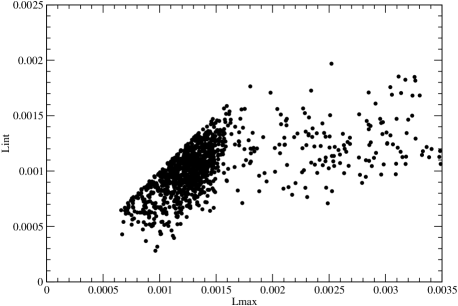
Figure 4: $L_{max}$ versus $L_{int}$ for Model E5c. Only the region of low values, around the region corresponding to regular orbits is shown.

Now, that $L_{lim}$ corresponds to a Lyapunov time of $556\>t.u.$, which is equivalent to about 5 or 6 Hubble times for our models. Is it reasonable to use such a low $L_{lim}$ to separate regular from chaotic orbits? Would it not be more sensible to adopt a value of $0.0100\>(t.u.)^{-1}$ which corresponds to a Lyapunov time of the same order of the Hubble time? Those questions have been considered in our previous work (see Aquilano et al., 2007; , Muzzio et al.2009, for example) and we will repeat here the same analysis done there.

First, we separated the orbits of each model into three groups: a) Those with $Lmax<0.0018\>(t.u.)^{-1}$, i.e., those that are classified as regular for both choices of $L_{lim}$ (REGREG, hereafter); b) Those with $0.0018\>(t.u.)^{-1}\leavevmode\nobreak\ \leq\leavevmode\nobreak\ L_{max}\leavevmode\nobreak\ <\leavevmode\nobreak\ 0.0100\>(t.u.)^{-1}$, i.e., those that are classified as regular for $L_{lim}=0.0100\>(t.u.)^{-1}$, but as chaotic for $L_{lim}=0.0018\>(t.u.)^{-1}$ (REGCHAO, hereafter); c) Those with $0.0100\>(t.u.)^{-1}\leavevmode\nobreak\ \leq\leavevmode\nobreak\ L_{max}$, ie, those that are classified as chaotic for both elections of $L_{lim}$ (hereafter CHAOCHAO). Then we considered, for each orbit, 11 $(x,\leavevmode\nobreak\ y,\leavevmode\nobreak\ z)$ orbital positions separated by intervals of $10\>t.u.$, that is, over a total interval of $100\>t.u.$, and, for each model and for each type of orbit, we computed the mean square value of each coordinate. Table  6 gives the square roots of the ratios of the $y$ and $z$ mean square values to the $x$ mean square value.

Table 6: Axial ratios of different classes of orbits for different choices of $L_{lim}$.

$Ratio$	$Mod$	$REGREG$	$REGCHAO$	$CHAOCHAO$
y/x	E2a	1.030 $\pm$ 0.015	0.868 $\pm$ 0.013	0.865 $\pm$ 0.015
	E2b	1.023 $\pm$ 0.014	0.868 $\pm$ 0.013	0.875 $\pm$ 0.015
	E2c	1.003 $\pm$ 0.014	0.847 $\pm$ 0.014	0.856 $\pm$ 0.014
	E3a	0.816 $\pm$ 0.022	0.851 $\pm$ 0.018	0.856 $\pm$ 0.018
	E3b	0.815 $\pm$ 0.023	0.824 $\pm$ 0.019	0.829 $\pm$ 0.017
	E3c	0.773 $\pm$ 0.025	0.866 $\pm$ 0.018	0.877 $\pm$ 0.016
	E4a	0.520 $\pm$ 0.040	0.745 $\pm$ 0.026	0.874 $\pm$ 0.019
	E4b	0.510 $\pm$ 0.044	0.788 $\pm$ 0.028	0.841 $\pm$ 0.019
	E4c	0.568 $\pm$ 0.039	0.765 $\pm$ 0.023	0.830 $\pm$ 0.019
	E5a	0.892 $\pm$ 0.028	0.877 $\pm$ 0.025	0.908 $\pm$ 0.018
	E5b	0.965 $\pm$ 0.026	0.833 $\pm$ 0.025	0.899 $\pm$ 0.018
	E5c	0.934 $\pm$ 0.029	0.759 $\pm$ 0.025	0.839 $\pm$ 0.016
z/x	E2a	0.910 $\pm$ 0.016	0.915 $\pm$ 0.013	0.905 $\pm$ 0.015
	E2b	0.937 $\pm$ 0.015	0.903 $\pm$ 0.013	0.874 $\pm$ 0.015
	E2c	0.879 $\pm$ 0.015	0.928 $\pm$ 0.014	0.891 $\pm$ 0.014
	E3a	0.676 $\pm$ 0.024	0.840 $\pm$ 0.018	0.832 $\pm$ 0.019
	E3b	0.712 $\pm$ 0.027	0.812 $\pm$ 0.018	0.771 $\pm$ 0.018
	E3c	0.668 $\pm$ 0.028	0.851 $\pm$ 0.018	0.823 $\pm$ 0.017
	E4a	0.424 $\pm$ 0.053	0.719 $\pm$ 0.028	0.760 $\pm$ 0.020
	E4b	0.353 $\pm$ 0.044	0.660 $\pm$ 0.028	0.767 $\pm$ 0.019
	E4c	0.401 $\pm$ 0.049	0.710 $\pm$ 0.026	0.769 $\pm$ 0.020
	E5a	0.309 $\pm$ 0.033	0.501 $\pm$ 0.031	0.759 $\pm$ 0.021
	E5b	0.361 $\pm$ 0.040	0.527 $\pm$ 0.035	0.699 $\pm$ 0.020
	E5c	0.319 $\pm$ 0.043	0.473 $\pm$ 0.032	0.699 $\pm$ 0.018

The results in Table 6 show that, as in our previous work, most of the axial ratios of the REGCHAO orbits are significantly different from those of the REGREG orbits and we may conclude that, despite their low FT-LCN values implying Lyapunov times longer than the Hubble time, orbits with $0.0018\>(t.u.)^{-1}\leq L_{max}<0.0100\>(t.u.)^{-1}$ have a spatial distribution different from that of regular orbits. In other words, the time scale for the exponential divergence of orbits (measured by the Lyapunov time) is not much relevant for the spatial distribution of those orbits. Since we are here interested in that distribution, the sensible approach is thus to adopt $L_{lim}=0.0018\>(t.u.)^{-1}$. Therefore, we classify orbits as regular if $L_{max}\leavevmode\nobreak\ <\leavevmode\nobreak\ L_{lim}$, as partially chaotic if $L_{int}\leavevmode\nobreak\ <\leavevmode\nobreak\ L_{lim}\leavevmode\nobreak\ \leq\leavevmode\nobreak\ L_{max}$ and as fully chaotic if $L_{lim}\leavevmode\nobreak\ \leq\leavevmode\nobreak\ L_{int}$.

Table 7 gives the percentages of regular, partially and fully chaotic orbits in our models. As in our previous works, the statistical errors have been estimated from the binomial distribution. The agreement among results of the a, b and c cases of each model is excellent and within the $3\sigma$ level in all cases, except for the regular and fully chaotic orbits of the E3c case where the differences with the E3a and E3b cases are of the order of $5\sigma$. Clearly, all our models harbor the lowest fractions of regular orbits in triaxial systems we know about, lower even than the $29.05$ per cent found by (Muzzio et al.2009) for their model E6c. Interestingly, the fraction of regular orbits does not decrease monotonically from type E2 through type E5, but falls first to rise again; a somewhat similar, but less pronounced, trend was found in the E4 through E6 models of Aquilano et al. (2007). The decreasing fractions of partially chaotic orbits when going from type E2 through E5 show the same trend found in those two previous works of ours.

Two further tests were performed to check the accuracy of our results. On the one hand, it is interesting to check the influence that the use of a particular N-body snapshot as a model might have. On the other hand, since we are using only about 0.5 per cent of the orbits in each model to investigate chaoticity, it might be worthwile to see if the use of a different sample yields different results. We adopted the E4b model for both tests. For the first one, we took a new model from the snapshot evolved $200T_{cr}$ more than the one whose results are presented in Table 7, and we obtained fractions of $14.42\pm 0.52\%$, $11.95\pm 0.48\%$ and $73.62\pm 0.65\%$, respectively for the regular, partially and fully chaotic orbits. The first two fractions coincide with those of the original model at the $3\sigma$ level, but the last one differs by $3.4\sigma$. Not only are these differences small, but they are probably at least partially due to the axial changes of the models as they evolve described in Subsection 3.1. The $200T_{cr}$ evolution changes the triaxiality of the E4b model in the direction of that of the E5 models by about $1/10$ of the triaxiality difference between the E4 and E5 models. Since the difference between the fractions of fully chaotic orbits of those models is about $8\%$ we might crudely estimate that about $0.8\%$ of the change from the original model to the one evolved $200T_{cr}$ might be attributed to the axial changes, in which case the remaining difference is of $2.5\sigma$ only. Nevertheless, the agreement between the original and the $200T_{cr}$ evolution results is somewhat poorer than those among statistically different realizations of the same model, except for the already mentioned differences for models E3. The second test, instead, yielded no significant differences. The new sample of orbits from E4b model had fractions of $12.50\pm 0.49\%$, $9.74\pm 0.44\%$ and $77.76\pm 0.62\%$, respectively of regular, partially and full chaotic orbits, all of them well within the $3\sigma$ level of differences from the original results.

Table 7: Percentages of regular and chaotic orbits in triaxial systems.

$Mod$	$Regular(\%)$	$Part.\;Chaotic(\%)$	$Fully\;Chaotic(\%)$
E2a	22.48 $\pm$ 0.59	15.30 $\pm$ 0.51	62.22 $\pm$ 0.69
E2b	21.35 $\pm$ 0.58	15.52 $\pm$ 0.51	63.13 $\pm$ 0.69
E2c	22.24 $\pm$ 0.59	13.64 $\pm$ 0.49	64.12 $\pm$ 0.68
E3a	14.21 $\pm$ 0.50	13.19 $\pm$ 0.48	72.60 $\pm$ 0.64
E3b	14.04 $\pm$ 0.50	13.57 $\pm$ 0.49	72.39 $\pm$ 0.64
E3c	10.63 $\pm$ 0.44	12.90 $\pm$ 0.48	76.47 $\pm$ 0.61
E4a	13.05 $\pm$ 0.50	10.85 $\pm$ 0.46	76.10 $\pm$ 0.63
E4b	12.72 $\pm$ 0.50	10.58 $\pm$ 0.46	76.70 $\pm$ 0.63
E5c	12.67 $\pm$ 0.49	10.11 $\pm$ 0.45	77.22 $\pm$ 0.62
E5a	21.71 $\pm$ 0.61	9.69 $\pm$ 0.44	68.60 $\pm$ 0.69
E5b	23.06 $\pm$ 0.63	9.38 $\pm$ 0.43	67.96 $\pm$ 0.69
E5c	20.92 $\pm$ 0.60	8.86 $\pm$ 0.42	70.22 $\pm$ 0.68

The values of the FT-LCNs are larger than those we found for non-cuspy models, in agreement with the results of Kandrup & Sideris (2002) and Kandrup & Siopis (2003). Figure 5 shows, for our model E5c, the plot of $L_{max}$ versus the reduced energy (i.e., the orbital energy, E, divided by the potential energy at the galactic centre, $W_{o}$), which can be compared with Fig. 3 of (Muzzio et al.2005). In the present case the largest FT-LCNs are close to $1.0\>(t.u.)^{-1}$, while for the non-cuspy model of (Muzzio et al.2005) they only reached about $0.5\>(t.u.)^{-1}$. Besides, in the non-cuspy system there were no chaotic orbits for $E/W_{o}$ values close to $1.0$ (i.e., orbits very close to the centre of the system), because the potential near the centre was essentially that of a three dimensional harmonic oscillator. But, here, the presence of the cusp strongly limits the central region where the potential can be approximated with an integrable potential and, therefore, one can find chaotic orbits near the centre of the system.

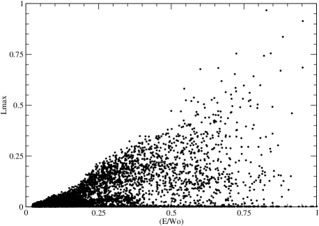
Figure 5: The maximum FT-LCNs ($L_{max}$) versus reduced orbital energy plot for Model E5c

For each model we took eleven orbital positions at intervals of $10\>t.u.$, i.e., over a total interval of $100\>t.u.$, to obtain the mean square values of each coordinate separately for each type of orbit. Table 8 gives the $y/x$ and $z/x$ axial ratios, computed from the square roots of those quadratic mean values. All the results for the a, b and c realizations of a same model show very good agreement at the $3\sigma$ level, except for the $y/x$ ratio difference between models E4b and E4c for the fully chaotic orbits, which is somewhat larger. The differences between the distributions of the partially and fully chaotic orbits are significant at the $3\sigma$ level only for $z/x$ ratio of the E5 models and the b case of models E4. This result agrees with those obtained for the models we studied before (Aquilano et al., 2007; , Muzzio et al.2009) in the sense that the differences between the distributions of partially and fully chaotic orbits, on the one hand, increased for more flattened systems and, on the other hand, diminished for cuspy systems.

Table 8: Axial ratios of different kinds of orbits.

$Ratio$	$Mod$	$Regular$	$Part.\;Chaotic$	$Fully\;Chaotic$
y/x	E2a	1.030 $\pm$ 0.015	0.903 $\pm$ 0.016	0.828 $\pm$ 0.014
	E2b	1.023 $\pm$ 0.014	0.899 $\pm$ 0.016	0.841 $\pm$ 0.014
	E2c	1.003 $\pm$ 0.014	0.891 $\pm$ 0.016	0.813 $\pm$ 0.014
	E3a	0.816 $\pm$ 0.022	0.878 $\pm$ 0.020	0.800 $\pm$ 0.024
	E3b	0.815 $\pm$ 0.023	0.863 $\pm$ 0.021	0.765 $\pm$ 0.027
	E3c	0.773 $\pm$ 0.025	0.915 $\pm$ 0.020	0.799 $\pm$ 0.025
	E4a	0.520 $\pm$ 0.040	0.804 $\pm$ 0.032	0.712 $\pm$ 0.032
	E4b	0.510 $\pm$ 0.044	0.781 $\pm$ 0.035	0.814 $\pm$ 0.034
	E4c	0.568 $\pm$ 0.039	0.894 $\pm$ 0.030	0.652 $\pm$ 0.029
	E5a	0.892 $\pm$ 0.028	0.869 $\pm$ 0.029	0.903 $\pm$ 0.018
	E5b	0.965 $\pm$ 0.026	0.868 $\pm$ 0.030	0.871 $\pm$ 0.017
	E5c	0.934 $\pm$ 0.029	0.790 $\pm$ 0.029	0.813 $\pm$ 0.016
z/x	E2a	0.910 $\pm$ 0.016	0.905 $\pm$ 0.016	0.919 $\pm$ 0.013
	E2b	0.937 $\pm$ 0.015	0.870 $\pm$ 0.016	0.917 $\pm$ 0.013
	E2c	0.879 $\pm$ 0.015	0.930 $\pm$ 0.016	0.903 $\pm$ 0.014
	E3a	0.676 $\pm$ 0.024	0.825 $\pm$ 0.021	0.867 $\pm$ 0.024
	E3b	0.712 $\pm$ 0.027	0.791 $\pm$ 0.021	0.831 $\pm$ 0.026
	E3c	0.668 $\pm$ 0.028	0.845 $\pm$ 0.022	0.850 $\pm$ 0.025
	E4a	0.424 $\pm$ 0.053	0.648 $\pm$ 0.037	0.798 $\pm$ 0.034
	E4b	0.359 $\pm$ 0.045	0.573 $\pm$ 0.037	0.789 $\pm$ 0.033
	E4c	0.401 $\pm$ 0.049	0.699 $\pm$ 0.036	0.730 $\pm$ 0.031
	E5a	0.309 $\pm$ 0.033	0.374 $\pm$ 0.033	0.733 $\pm$ 0.020
	E5b	0.361 $\pm$ 0.040	0.484 $\pm$ 0.045	0.675 $\pm$ 0.019
	E5c	0.319 $\pm$ 0.043	0.398 $\pm$ 0.038	0.671 $\pm$ 0.018

4 Conclusions

The method of Hernquist & Ostriker (1992) is clearly better than that of Aguilar (Aguilar & Merritt, 1990) to build cuspy triaxial stellar models, since the former needs no softening and uses a radial expansion which is particularly adequate to fit N–body distributions with $\gamma\simeq 1$. As a side benefit, the coefficients of both the radial and angular expansions are provided by the method itself and there is no need of additional fittings to obtain them. The only caveat is that, as shown by (Kalapotharakos et al.2008), the method of Hernquist and Ostriker is adequate for cases with $\gamma\simeq 1$ only and, for other slopes of the cusp, other related but different methods should be preferred.

The models obtained using the same parameters and changing only the seed number of the random number generator show that our results are very robust, indeed. Those models exhibit essentially the same global properties (except for the angular velocity of figure rotation) and, with very few exceptions, the same fractions and distributions of regular, partially and fully chaotic orbits. The different angular velocities we obtained here for statistically equivalent models further complicates the little we know about the phenomenon of figure rotation (i.e., with zero angular momentum) in this kind of models. On the one hand, the reality of the rotation has been checked using both the Aguilar (Aguilar & Merritt, 1990) and Aarseth (Aarseth, 2003) codes by Muzzio (2006) and here with the Hernquist code and, on the other hand, such triaxial systems with figure rotation are just the stellar equivalent of the Riemann ellipsoids of fluid dynamics, so that there is nothing misterious about their existence. Nevertheless, except for the increase of the angular velocity when one goes to flatter systems, the rotation does not seem to correlate with other properties of the systems and, moreover, now it turns out that statistically equivalent systems have different velocities. Even though, as already indicated, the angular velocities are so low that they have very little effect on orbital chaoticity, this phenomenon is interesting and warrants further investigation.

The high stability of our models over time scales of the order of a Hubble time is very well stablished. Not only are the detected variations very small, but they are most likely due to relaxation effects of the N–body code. Besides, it should be stressed that we have checked the stability running the models self-consistently, while checks on the stability of models resulting from the method of Schwarzschild (1979) are usually done on fixed potentials (Schwarzschild, 1993). As we have shown, when the potential is fixed, the changes in our models are an order of magnitude smaller than those found self-consistently.

Although, considering the results of Kandrup & Sideris (2002), Kandrup & Siopis (2003) and (Muzzio et al.2009), high fractions of chaotic orbits could be expected in our cuspy triaxial models, the fractions found are extremely high, indeed, exceeding $85$ per cent for our E2 and E3 models. It is important to emphasize that those high fractions of chaotic orbits are not merely due to the low $L_{lim}$ adopted: Had we adopted the $0.010\>(t.u.)^{-1}$ limit, those models would still have had between $70$ an $75$ per cent of chaotic orbits.

The main conclusion of our investigation is that it is perfectly possible to build self-consistent stellar models of cuspy triaxial elliptical galaxies that are very stable despite containing high percentages of chaotic orbits. This result confirms and extends previous work by others (, Voglis et al.2002; Kalapotharakos & Voglis, 2005) and ours (Aquilano et al., 2007; , Muzzio et al.2009). It also supports the suggestion by (Muzzio et al.2005) in the sense that the difficulties to obtain such models with the method of Schwarzschild should be attributed to the method itself and not to physical causes. It is true that, while regular orbits always occupy the same region of space, chaotic orbits may spend a long interval occupying certain region, only to switch to a different one later on, with sticky orbits being an extreme example. But, although such behaviour conspires against obtaining stable models with high fractions of chaotic orbits with the method of Schwarzschild, it does not necessarily prevents the existence of those models. All one needs is that, as some chaotic orbits abandon a region of space to explore a different one, orbits in the latter region move on to replace those in the former. In other words, rather than having a static equilibrium, with each orbit covering always the same zone, we have a dynamic equilibrium where switches from one zone to another are present but balance each other on average. Our models show that such state of affairs is perfectly possible.

5 Acknowledgements

We are very grateful to Lars Hernquist and Daniel Pfenniger for allowing us to use their codes, to C. Efthymiopoulos for useful comments, to H.D. Navone for his assistance with programming, to R.E. Martínez and H.R Viturro for their technical assistance and to an anonymous referee for his comments on the original version of the present paper. This work was supported with grants from the Consejo Nacional de Investigaciones Científicas y Técnicas de la República Argentina, the Agencia Nacional de Promoción Científica y Tecnológica, The Universidad Nacional de La Plata and the Universidad Nacional de Rosario.

References

- Aarseth (2003) Aarseth S.J., 2003, Gravitational N–body Simulations, Cambridge University Press, Cambridge
- Aguilar & Merritt (1990) Aguilar L.A., Merritt D., 1990, ApJ, 354, 33
- Aquilano et al. (2007) Aquilano R.O., Muzzio J.C., Navone H.D., Zorzi A.F., 2007, Celestial Mech. Dyn. Astr., 99, 307
- Binney & Tremaine (2008) Binney J., Tremaine S.J., 2008, Galactic Dynamics, Princeton University Press
- Capuzzo–Dolcetta et al. (2007) Capuzzo–Dolcetta R., Leccese L., Merritt D., Vicari A., 2007, ApJ, 666, 165
- Cincotta et al. (2003) Cincotta P.M., Giordano C.M., Simó C., 2003, Physica D, 182, 151
- Contopoulos (2004) Contopoulos G., 2004, Order and Chaos in Dynamical Astronomy, Springer
- Dehnen (1993) Dehnen W., 1993, MNRAS, 265, 250
- Forbes & Ponman (1999) Forbes D.A., Ponman T.J., 1999, MNRAS, 309, 623
- Hernquist (1990) Hernquist L., 1990, ApJ, 356, 359
- Hernquist & Barnes (1990) Hernquist L., Barnes J., 1990, ApJ, 349, 562
- Hernquist & Ostriker (1992) Hernquist L., Ostriker J.P., 1992, ApJ, 386, 375
- Holley–Bockelmann et al. (2001) Holley–Bockelmann K., Mihos J.C., Sigurdsson S., Hernquist L., 2001, ApJ, 549, 862
- Jesseit et al. (2005) Jesseit R., Naab T., Burkert A., 2005, MNRAS, 360, 1185
- (15) Kalapotharakos C., Efthymiopoulos C., Voglis N., 2008, MNRAS, 383, 971
- Kalapotharakos & Voglis (2005) Kalapotharakos C., Voglis N., 2005, Celestial Mech. Dyn. Astr., 92(1–3), 157
- Kandrup & Sideris (2002) Kandrup H.E., Sideris I.V., 2002, Celestial Mech. Dyn. Astr., 82
- Kandrup & Siopis (2003) Kandrup H.E., Siopis C., 2003,MNRAS, 345, 727
- Merritt & Fridman (1996) Merritt D., Fridman T., 1996, ApJ, 460(1), 136
- Muzzio (2006) Muzzio J.C., 2006, Celestial Mech. Dyn. Astr., 96(2), 85
- (21) Muzzio J.C., Carpintero D.D., Wachlin F.C., 2005, Celestial Mech. Dyn. Astr., 91(1-2), 173
- (22) Muzzio J.C., Navone H.D., Zorzi A.F., 2009, Celestial Mech. Dyn. Astr., 105(4), 379
- Napolitano et al. (2005) Napolitano N.R. et al., 2005, MNRAS, 357, 691
- Schwarzschild (1979) Schwarzschild M., 1979, ApJ, 232, 236
- Schwarzschild (1993) Schwarzschild M., 1993, ApJ, 409, 563
- Siopis & Kandrup (2000) Siopis C., Kandrup H.E., 2000, MNRAS, 319, 43
- Sparke & Sellwood (1987) Sparke L.S., Sellwood J.A., 1987, MNRAS, 225, 653
- Udry & Pfenniger (1988) Udry S., Pfenniger D., 1988, A&A, 198(1–2), 135
- (29) Voglis N., Kalapotharakos C., Stavropoulos I., 2002, MNRAS, 337(2), 619
- White (1983) White S.D.M., 1983, ApJ, 274, 53
- Zorzi & Muzzio (2009) Zorzi A. F., Muzzio J. C., 2009, Memorias del II Congreso de Matemática Aplicada, Computacional e Industrial, Rosario (2009)